Bidirectional optical non-reciprocity in a multi-mode cavity optomechanical system

Abstract

Optical non-reciprocity that allows unidirectional flow of optical field is pivoted on the time reversal symmetry breaking, which originates from radiation pressure because of light-matter interaction in cavity optomechanical systems. Here, the non-reciprocal transport of optical signals across two ports via three optical modes optomechanically coupled to the mechanical excitation of two nanomechanical resonators (NMRs) is studied under the influence of strong classical drive fields and weak probe fields. It is found that there exists the conversion of reciprocal to non-reciprocal signal transmission via tuning the drive fields and perfect non-reciprocal transmission of output fields can be realized when the effective cavity detuning parameters are near resonant to the NMRs’ frequencies. The unidirectional non-reciprocal transport is robust to the optomechanical couplings around resonance conditions. Moreover, the cavities’ photon loss rates play an inevitable role in the unidirectional flow of signal across the two ports. Bidirectional transmission can also be controlled by the phase changes associated with the probe and drive fields along with their relative phase. This scheme may provide a foundation for the compact non-reciprocal communication and quantum information processing, thus enabling novel devices that route photons in unconventional ways such as all-optical diodes, optical transistors and optical switches.

Muhib Ullah Xihua Yang Li-Gang Wang*

Dr. M. Ullah,
Department of Physics, Zhejiang University, Hangzhou 310027, China
Prof. X. Yang,
Department of Physics, Shanghai University, Shanghai 200444, China

Prof. L.-G. Wang
Department of Physics, Zhejiang University, Hangzhou 310027, China
Canadian Quantum Research Center, 204-3002 32 Ave, Vernon, BC V1T 2L7, Canada
Email Address:lgwang@zju.edu.cn

1 Introduction

Non-reciprocity is a phenomenon in certain devices that allows signal to pass through in one direction, but block it in the opposite, and is requisite in a broad range of applications such as invisibility or cloaking, and noise free information processing. ¹ Optical non-reciprocity has originated from breaking the Lorentz reciprocity theorem. ² Apart from that, optical non-reciprocity has been realized in magneto-optical Faraday effect, ^{3, 4, 5, 6, 7, 8, 9} but the major flaw in these devices is their inconvenience in integration because of some issues such as cross talk caused by the magnetic field, ill-suitableness for sensitive superconducting circuits as their strong magnetic fields are highly disruptive and need strong shielding, and lattice mismatches between magneto-optical materials and silicon. ¹⁰ In addition, magneto-optical materials manifest remarkable loss at optical frequencies, that is, the order of 100 dB cm^-1, making them sub-optimal solutions for high efficiency devices. As an alternate to the magneto-optical non-reciprocal devices, several techniques have been practiced by using microwave chip-level systems. One approach is based on an artificial magnetic field by modulating the parametric coupling between the modes of a network, thus making the system non-reciprocal at the ports. ^{11, 12} Second technique is the phase matching of a parametric interaction that leads to non-reciprocal behavior of the communicating signal, since the signal only interacts with the pump when co-propagating with it and not in the opposite direction. This causes traveling-wave amplification to be directional. ^{13, 14, 15, 16}

The approach for on-chip optical non-reciprocity has also been used recently by using a strong optomechanical interaction between the external fields and micro-ring resonators, ¹⁷ and this has been experimentally demonstrated using a silica microsphere resonator. ¹⁸ The optomechanical interaction basically arises from the radiation pressure between cavity photons and mechanical resonators in an optomechanical cavity whose details can be found in a recent review by Meystre. ¹⁹ Using the three-mode optomechanical system, Chen et al., have proposed a scheme for non-reciprocal mechanical squeezing due to the joint effect of the mechanical intrinsic nonlinearity and the quadratic optomechanical coupling. ²⁰ In a similar fashion, an optomechanical circulator and directional amplifier in a two-tapered fiber-coupled silica micro-resonator have been proposed to perform as an add-drop filter, and they may be switched to circulator mode or directional amplifier mode via a simple change in the control field. ²¹ It has been accredited that the non-reciprocal signal transfer between two optical modes mediated by mechanical mode can be realized with suitable optical driving. ^{22, 23} Additionally, these modes in cavity optomechanics can also result in some other interesting effects like ground-state cooling of a NMR, ^{24, 25} steady-state light-mechanical quantum steerable correlations in a cavity optomechanical system (COS), ²⁶ slow-to-fast light tuning and single-to-double optomechanically induced transparency (analogous to electromagnetically induced transparency), ²⁷ flexible manipulation on Goos-H$\ddot{\rm{a}}$nchen shift as a classical application of COS, ²⁸ Fano resonances, ²⁹ superradiance, ³⁰ optomechanically induced opacity and amplification in a quadratically coupled COS, ³¹ and they can also be used for non-classical state generation in cavity QED when atom interacts with the cavity dynamics to induce large nonlinearity in the system. ³² Similarly, by tailoring the fluctuations of driving fields in an optomechanical system with a feedback loop, the performance of optomechanical system is greatly improved.  ³³ Apart from that, Peterson et al., have further demonstrated an efficient frequency-converting microwave isolator, stemmed on the optomechanical interactions between electromagnetic fields and a mechanically compliant vacuum-gap capacitor, which does not require a static magnetic field and allows a dynamic control of the direction of isolation. ³⁴ Bernier et al., have experimentally realized the non-reciprocal scheme in an optomechanical system using a superconducting circuit in which mechanical motion is capacitively coupled to a multi-mode microwave circuit. ³⁵ Similarly, Barzanjeh et al., have presented an on-chip microwave circulator using a frequency tunable silicon-on-insulator electromechanical system to investigate non-reciprocity via two output ports and is also compatible with superconducting qubits. ³⁶

Fetching an insight from the above discussion, we introduce a scheme to achieve bidirectional non-reciprocal signal transmission using purely optomechanical interactions in the presence of a partial beam splitter (BS). The setup consists of two ports (left and right) through which the signal exchange occurs. The external fields interact with the cavity modes and thus with the nanomechanical resonators’ (NMRs) phonons via radiation pressure forces, which induce effective nonlinearity into the system and breaks the time reversal symmetry. These factors are ultimately accountable for the optical non-reciprocal behavior of the system to incoming light fields. Non-reciprocal process as a result of interference due to different phases has been discussed in a two-mode cavity system with two mechanical modes. ^{37, 38} Very recently, in a letter, a configurable and directional electromagnetic signal transmission has been shown to be obtained in an optomechanical system by designing a loop of interactions in the synthetic plane generated by driven Floquet modes on one hand and multiple mechanical modes on the other hand, to realize a microwave isolator and a directional amplifier. ³⁹

This work is organized as follows. In section 2, we present the model of multi-mode COS and calculate the analytical results for the output fields of both ports 1 and 2. In section 3, we analyze and discuss our results numerically and explain the non-reciprocal behavior of output signals under different system parameters. In the last section 4, we conclude our work.

2 Model and Calculations

The proposed model shown in Figure 1 is a two-port COS that is composed of two partially transparent mirrors (M₁ and M₂) fixed opposite to each other and two perfectly reflecting movable NMRs oscillating along the same axis and a 50:50 partial BS is placed between them. The NMRs oscillate around their equilibrium positions with small displacements $q_{1}$ and $q_{2}$, usually in the order of 10^-9 m or even lower, ⁴⁰ which is much smaller than the characteristic wavelengths of cavity modes. Thus, different cavity modes are essentially determined by their own cavity lengths. According to Figure 1, there are three cavity modes, $a_{1}$, $a_{2}$ and $a_{3}$, interacting with the NMRs. Modes $a_{1}$ and $a_{2}$ are, respectively, formed independently between the fixed mirrors M_1,2 and the NMR_1,2, while the cavity mode $a_{3}$ is also formed between NMR₁ and NMR₂ via the BS. Here we assume that all these cavity modes have different frequencies since the cavity lengths are unlike in general. The last cavity mode between two fixed mirrors M₁ and M₂ can be neglected since it does not have any interaction with those NMRs. To control or manipulate the proposed COS, two external classical and strong driving fields with field strengths $\Omega_{d1},\leavevmode\nobreak\ \Omega_{d2}$ and the same frequency $\omega_{d}$ and the two weak probe fields with field strengths $\Omega_{p1},\leavevmode\nobreak\ \Omega_{p2}$ and the same frequency $\omega_{p}$ are injected from both ports (left and right) to the COS setup. Since the NMRs are supposed to be perfect reflecting mirrors and a 50:50 partial BS exists in the setup, all these driving and probe fields exist in the whole setup and interact with those three cavity modes $a_{1}$, $a_{2}$ and $a_{3}$. After interacting with the cavity dynamics, the output probe fields ($\varepsilon_{\rm{out,1}},\leavevmode\nobreak\ \varepsilon_{\rm{out,2}}$) can be collected at the left and right ports, respectively.

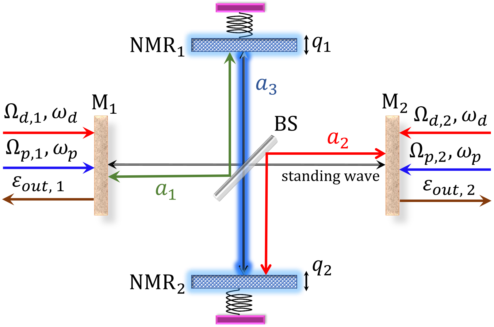
Figure 1: Schematic of a two ports multi-mode optomechanical cavity setup excited by external classical fields. The setup includes two fixed partially transparent mirrors (M₁ and M₂) and two movable perfectly reflecting nano-mechanical resonators (NMR₁ and NMR₂) with small displacements $q_{1}$ and $q_{2}$ from their respective equilibrium positions. A partial BS is placed at the center inside the mirrors configuration which form three uneven cavity modes. These cavity modes, that is, $a_{1}$, $a_{2}$ and $a_{3}$, and two mechanical (phononic) modes ($b_{1}$ and $b_{2}$) in this system are interconnected via optomechanical couplings, while a standing wave between M₁ and M₂ being represented by a straight horizontal arrow is formed. Four classical fields, i.e., strong drive fields with strengths $\Omega_{d1}$ and $\Omega_{d2}$ (same frequency $\omega_{d}$), and weak probe fields having strengths $\Omega_{p1}$ and $\Omega_{p2}$ (same frequency $\omega_{p}$) interact with the cavity system from the respective sides via M₁ and M₂, while the output fields ($\varepsilon_{\rm{out,1}}$ and $\varepsilon_{\rm{out,2}}$) can be drawn out via left and right ports, respectively.

The Hamiltonian for this COS in the frame rotating at the drive field frequency $\omega_{d}$ can be given as

$$H_{T}= \sum_{i=1}^{3}\Delta_{ai}a_{i}^{\dagger}a_{i}+\sum_{j=1}^{2}\omega_{mj}b_{j}^{\dagger}b_{j}+\sum_{i=1}^{2}O_{mi}a_{i}^{\dagger}a_{i}(b_{i}^{\dagger}+b_{i})+O_{m31}a_{3}^{\dagger}a_{3}(b_{1}^{\dagger}+b_{1})+O_{m32}a_{3}^{\dagger}a_{3}(b_{2}^{\dagger}+b_{2})$$

$$+\sum_{j=1}^{2}\sum_{k=1}^{3}i\Omega_{dj}(e^{i\Phi_{dj}}a_{k}^{\dagger}-e^{-i\Phi_{dj}}a_{k})+\sum_{j=1}^{2}\sum_{k=1}^{3}i{\Omega_{pj}}(e^{-i(\Delta_{p}t-\Phi_{pj})}a_{k}^{\dagger}-\rm{H.c.})$$ (1)

where $\Delta_{a1}=\omega_{a1}-\omega_{d}$, $\Delta_{a2}=\omega_{a2}-\omega_{d}$ and $\Delta_{a3}=\omega_{a3}-\omega_{d}$ are the cavity-drive field detunings, whereas $\Delta_{p}=\omega_{p}-\omega_{d}$ denotes the probe-drive field detuning. In Hamiltonian of Equation (1), the first term stands for the energy of cavity modes $a_{i}$ with $i=1,2,3$ the $i$th cavity mode. The second term shows the energy of two bosonic modes $b_{j}$ with $j=1,2$ corresponding to two NMRs. The third term accounts for the optomechanical interactions between cavity modes ($a_{1,2}$) and mechanical modes ($b_{1,2}$) that come into existence because of radiation pressure, while the parameters $O_{mi}\leavevmode\nobreak\ (i=1,2)$ are the optomechanical coupling strengths between the cavity photons and NMRs. The fourth and fifth terms are associated with the optomechanical interaction between the cavity mode $a_{3}$ and two NMRs having $O_{m31}$ and $O_{m32}$ as the optomechanical couplings between them. These optomechanical couplings are crucial for the realization of optical non-reciprocity in our proposed cavity setup. Non-reciprocity is lost when these couplings vanish or become equal to zero. Here we emphasize that the hopping interactions between different cavity modes via the two NMRs cannot happen in general due to the uneven frequencies of these cavity modes ³⁷. The last two terms correspond to the interaction of strong classical drive fields and weak probe fields with the cavity modes, respectively, having H.c. as the Hermitian conjugate terms. The parameters $\Omega_{dj}$ and $\Omega_{pj}$ ($j=1,2$) are the drive and probe field strengths, respectively, and are considered to have real values for convenience.

Considering that the system may be dissipative, we use the Heisenberg’s equations of motion (so-called quantum Langevin equation) along with damping terms given as ^{41, 42}

$$\dot{Z}=-\frac{i}{\hbar}[Z,H_{T}]-\gamma Z+N$$ (2)

where $Z\in\leavevmode\nobreak\ (a_{1},a_{2},a_{3},b_{1},b_{2})$ is a general operator variable, $\gamma$ is the corresponding damping term, and the term $N$ is the quantum white noise (Brownian noise) resulting from the interaction of system with external bath. Without loss of generality, the reduced Planck’s constant ($\hbar$) is considered as equal to 1. We use Equation (2) to obtain the equation of motion for every operator variable and explore the dynamics of the system. By substituting Equation (1) into Equation (2) and introducing the factorization theorem, that is, $\langle ab\rangle=\langle a\rangle\langle b\rangle$ ^{41, 43}, the noise terms vanish since their average values lower to zero and we obtain the following mean-value equations.

$$\langle\dot{a}_{1}\rangle= -(\kappa_{1}+i\Delta_{a1})\langle a_{1}\rangle+iO_{m1}(\langle b_{1}^{\dagger}\rangle+\langle b_{1}\rangle)\langle a_{1}\rangle+\sum_{j=1}^{2}{\Omega_{dj}}e^{i\Phi_{dj}}+\sum_{k=1}^{2}{\Omega_{pj}}e^{-i(\Delta_{p}t-\Phi_{pk})}$$ (3a)

$$\langle\dot{a}_{2}\rangle= -(\kappa_{2}+i\Delta_{a2})\langle a_{2}\rangle+iO_{m2}(\langle b_{2}^{\dagger}\rangle+\langle b_{2}\rangle)\langle a_{2}\rangle+\sum_{j=1}^{2}{\Omega_{dj}}e^{i\Phi_{dj}}+\sum_{k=1}^{2}{\Omega_{pj}}e^{-i(\Delta_{p}t-\Phi_{pk})}$$ (3b)

$$\langle\dot{a}_{3}\rangle= -(\kappa_{3}+i\Delta_{a3})\langle a_{3}\rangle+iO_{m31}(\langle b_{1}^{\dagger}\rangle+\langle b_{1}\rangle)\langle a_{3}\rangle+iO_{m32}(\langle b_{2}^{\dagger}\rangle+\langle b_{2}\rangle)\langle a_{3}\rangle\sum_{j=1}^{2}{\Omega_{dj}}e^{i\Phi_{dj}}$$

$$+\sum_{k=1}^{2}{\Omega_{pj}}e^{-i(\Delta_{p}t-\Phi_{pk})}$$ (3c)

$$\langle\dot{b}_{1}\rangle= -(\gamma_{1}+i\omega_{m1})\langle b_{1}\rangle+{i}O_{m31}\langle a_{3}^{\dagger}\rangle\langle a_{3}\rangle$$ (3d)

$$\langle\dot{b}_{2}\rangle= -(\gamma_{2}+i\omega_{m2})\langle b_{2}\rangle+{i}O_{m32}\langle a_{3}^{\dagger}\rangle\langle a_{3}\rangle$$ (3e)

It is difficult to solve the master equation exactly because of the existence of the nonlinear terms. Hence, we apply the linearization approach by assuming that each operator in the system can be written as the sum of its mean value and a small fluctuation, i.e., applying an ansatz of the form given by  ^{44, 45, 46} $Z=Z_{s}+\delta Z,(Z\in a_{1},a_{2},a_{3},b_{1},b_{2})$, where $Z_{s}$ stands for the steady-state value and $\delta{Z}$ for the small fluctuations around the steady-state values of all the operator variables under observation. The fluctuations for each variable can be addressed as

$$\delta a_{1} \rightarrow\delta\tilde{a}_{1}e^{-i\Delta_{1}t}\leavevmode\nobreak\ \leavevmode\nobreak\ \delta a_{2}\rightarrow\delta\tilde{a}_{2}e^{-i\Delta_{2}t}$$

$$\delta a_{3} \rightarrow\delta\tilde{a}_{3}e^{-i\Delta_{3}t}\leavevmode\nobreak\ \leavevmode\nobreak\ \delta b_{1}\rightarrow\delta\tilde{b}_{1}e^{-i\omega_{m1}t}$$

$$\delta b_{2} \rightarrow\delta\tilde{b}_{2}e^{-i\omega_{m2}t}$$ (4)

where $\Delta_{i}\leavevmode\nobreak\ (i=1,2,3)$ is the effective cavity detuning and $\omega_{mj}\leavevmode\nobreak\ (j=1,2)$ is the NMR’s resonance frequency. As the drive fields are much stronger than the probe fields, we can use the conditions $\left|a_{is}\right|\gg\delta a_{i}$ $(i=1,2,3)$ and $\left|b_{js}\right|\gg\delta b_{j}$ ($j=1,2$) in the absence of the probe fields $\Omega_{p1}$ and $\Omega_{p2}$, and finally get the steady-state solutions according to the method in Ref. ⁴⁷

$$a_{1s}= \frac{\Omega_{d1}e^{i\Phi_{d1}}+\Omega_{d2}e^{i\Phi_{d2}}}{(\kappa_{1}+i\Delta_{1})},\leavevmode\nobreak\ b_{1s}=\frac{iO_{m31}\left|a_{3s}\right|^{2}}{(\gamma_{1}+i\omega_{m1})},$$ (5a)

$$a_{2s}= \frac{\Omega_{d1}e^{i\Phi_{d1}}+\Omega_{d2}e^{i\Phi_{d2}}}{(\kappa_{2}+i\Delta_{2})},\leavevmode\nobreak\ b_{2s}=\frac{iO_{m32}\left|a_{3s}\right|^{2}}{(\gamma_{2}+i\omega_{m2})},$$ (5b)

$$a_{3s}= \frac{\Omega_{d1}e^{i\Phi_{d1}}+\Omega_{d2}e^{i\Phi_{d2}}}{(\kappa_{3}+i\Delta_{3})}$$ (5c)

were $\Delta_{1}=\Delta_{a1}-{O_{m1}}(b_{1s}+b_{1s}^{\ast})$, $\Delta_{2}=\Delta_{a2}-O_{m2}(b_{2s}+b_{2s}^{\ast})$ and $\Delta_{3}=\Delta_{a3}-{O_{m31}}(b_{1s}+b_{1s}^{\ast})-{O_{m32}}(b_{2s}+b_{2s}^{\ast})$ are the effective cavity detunings of the cavity modes $a_{1}$, $a_{2}$ and $a_{3}$, respectively. In Equation (5a)-(5c), the expressions $a_{is}$ ($i=1,2,3$) and $b_{js}$ ($j=1,2$) are the steady-state solutions of optical modes and mechanical modes, respectively. To find out the role of the weak probe fields in the system dynamics, the small fluctuations are taken into consideration by using the assumption given in Equation (4), and only slowly moving linear terms are entertained, while fast oscillating terms are ignored. Thus, the linearized equations of motion for the fluctuation part of the variable operators can be derived as

$$\delta\dot{\tilde{a}}_{1}= -(\kappa_{1}+i\Delta_{a1})\delta\tilde{a}_{1}+iO_{m1}a_{1s}\delta\tilde{b}_{1}+\Omega_{p1}e^{i\Phi_{p1}}e^{-ix_{1}t}+\Omega_{p2}e^{i\Phi_{p2}}e^{-ix_{1}t}$$ (6)

where $x_{1}=\omega_{p}-\omega_{d}-\omega_{m1}=\Delta_{p}-\omega_{m1}$ is the probe detuning and the movable mirror resonance frequency’s difference. Expressions for $\delta\dot{\tilde{a}}_{2}$ and $\delta\dot{\tilde{a}}_{3}$ can be solved alike as $\delta\dot{\tilde{a}}_{1}$, and they are given as

$$\delta\dot{\tilde{a}}_{2}= -(\kappa_{2}+i\Delta_{a2})\delta\tilde{a}_{2}+iO_{m2}a_{2s}\delta\tilde{b}_{2}+\Omega_{p1}e^{i\Phi_{p1}}e^{-ix_{2}t}+\Omega_{p2}e^{i\Phi_{p2}}e^{-ix_{2}t}$$ (7)

$$\delta\dot{\tilde{a}}_{3}= -(\kappa_{3}+i\Delta_{a3})\delta\tilde{a}_{3}+iO_{m31}a_{3s}\delta\tilde{b}_{1}+iO_{m32}a_{3s}\delta\tilde{b}_{2}+\Omega_{p1}e^{i\Phi_{p1}}e^{-ix_{3}t}+\Omega_{p2}e^{i\Phi_{p2}}e^{-ix_{3}t}$$ (8)

where the parameters $x_{2}=\Delta_{p}-\omega_{m2}$ and $x_{3}=\Delta_{p}-\Delta_{3}$. Without loss of generality, all the cavity modes are supposed to be driven in the mechanical red sidebands with $\Delta_{1}=\Delta_{2}=\Delta_{3}=\omega_{m1}=\omega_{m2}=\omega_{m}$. Therefore, $x_{1}=x_{2}=x_{3}=x$ and the system is operated in the resolved sideband regime with the condition that $\omega_{m}\gg{\kappa_{j}}$, where $j=1,2,3$. With the above assumptions, the coefficients of mechanical mode fluctuation operators $\delta\dot{\tilde{b}}_{1}$ and $\delta\dot{\tilde{b}}_{2}$ can be simplified as

$$\delta\dot{\tilde{b}}_{1} =-(\gamma_{1}+i\omega_{m1})\delta\tilde{b}_{1}+{i}O_{m31}a_{3s}^{\ast}\delta\tilde{a}_{3}$$ (9)

$$\delta\dot{\tilde{b}}_{2} =-(\gamma_{2}+i\omega_{m2})\delta\tilde{b}_{2}+{i}O_{m32}a_{3s}^{\ast}\delta\tilde{a}_{3}$$ (10)

The fluctuation values of the operator variables can be further expanded to obtain the solution easily by using the ansatz given below.

$$\delta\tilde{y}=\delta\tilde{y}_{+}e^{-ixt}+\delta\tilde{y}_{-}e^{ixt}$$ (11)

where $\delta\tilde{y}=\delta\tilde{a}_{1},\delta\tilde{a}_{2},\delta\tilde{a}_{3},\delta\tilde{b}_{1},\text{and}\leavevmode\nobreak\ \delta\tilde{b}_{2}$ are the fluctuation variables under study. By substituting Equation (11) into Equations (6)-(10), we achieve the simplified fluctuation operator coefficients for the optical cavity modes as

$$\delta\tilde{a}_{1+} =\frac{iO_{m1}a_{1s}\delta\tilde{b}_{1+}+\sum\limits_{j=1}^{2}\Omega_{pj}e^{i\Phi_{pj}}}{(\kappa_{1}+i\Delta_{a1}-ix)}$$ (12)

$$\delta\tilde{a}_{2+} =\frac{iO_{m2}a_{2s}\delta\tilde{b}_{2+}+\sum\limits_{j=1}^{2}\Omega_{pj}e^{i\Phi_{pj}}}{(\kappa_{2}+i\Delta_{a2}-ix)}$$ (13)

$$\delta\tilde{a}_{3+} =\frac{iO_{m31}a_{3s}\delta\tilde{b}_{1+}+iO_{m32}a_{3s}\delta\tilde{b}_{2+}+\sum\limits_{j=1}^{2}\Omega_{pj}e^{i\Phi_{pj}}}{(\kappa_{3}+i\Delta_{a3}-ix)}$$ (14)

whereas, expressions for the coefficients associated with the mechanical mode fluctuation operators can be calculated and simplified in similar fashion by substituting Equation (11) into Equation (6)-(10) and can be written as

$$\delta\tilde{b}_{1+} =\frac{iO_{m31}a_{3s}^{\ast}\delta\tilde{a}_{3+}}{(\gamma_{1}+i\omega_{m1}-ix)}$$ (15)

$$\delta\tilde{b}_{2+} =\frac{iO_{m32}a_{3s}^{\ast}\delta\tilde{a}_{3+}}{(\gamma_{2}+i\omega_{m2}-ix)}$$ (16)

As the transmission happens via fixed mirrors (left $\text{M}_{1}$ and right $\text{M}_{2}$) that are connected to the cavity modes $a_{1}$ and $a_{2}$, respectively, we calculate the corresponding coefficients $\delta\tilde{a}_{1+}$ and $\delta\tilde{a}_{2+}$. Therefore, we apply a lengthy and tiresome but straightforward substitution method to Equations (12)-(16) and obtain the required analytical expressions for $\delta\tilde{a}_{1+}$ and $\delta\tilde{a}_{2+}$ as

$$\delta\tilde{a}_{1+}=-\frac{D[V_{2}\zeta+\left|a_{3s}\right|^{2}(O_{m31}^{2}V_{2}+O_{m32}^{2}V_{1})]}{U_{1}[U_{3}V_{1}V_{2}+\left|a_{3s}\right|^{2}(O_{m31}^{2}V_{2}+O_{m32}^{2}V_{1})]}$$ (17)

$$\delta\tilde{a}_{2+}=-\frac{D[V_{1}\zeta^{\prime}+\left|a_{3s}\right|^{2}(O_{m31}^{2}V_{2}+O_{m32}^{2}V_{1})]}{U_{2}[U_{3}V_{1}V_{2}+\left|a_{3s}\right|^{2}(O_{m31}^{2}V_{2}+O_{m32}^{2}V_{1})]}$$ (18)

where $\zeta=U_{3}V_{1}-O_{m1}O_{m31}a_{1s}a_{3s}^{*}$, $\zeta^{\prime}=O_{m2}O_{m32}a_{2s}a_{3s}^{*}+U_{3}V_{2}$, $D=\Omega_{p1}e^{i\Phi_{p1}}+\Omega_{p2}e^{i\Phi_{p2}}$, while $U_{1}=ix-i\Delta_{a1}-\kappa_{1}$, $U_{2}=ix-i\Delta_{a2}-\kappa_{2}$, $U_{3}=ix-i\Delta_{a3}-\kappa_{3}$, $V_{1}=ix-i\omega_{m1}-\gamma_{1}$ and $V_{2}=ix-i\omega_{m2}-\gamma_{2}$ are the parametric symbols used in Equation (17) and (18).

To obtain output fields ($E_{\text{out},1}$ and $E_{\text{out},2}$) and study its non-reciprocal behavior through both the output ports in such an optomechanical system, input-output relation is convenient to be used as follows. ^{48, 49, 47}

$$E_{\text{out}}(t)+E_{\text{in}}(t)=2\kappa_{j}\langle\delta\tilde{a}_{j}\rangle$$ (19)

where $(j=1,2)$ and expression $E_{\text{out}}(t)=E_{\text{out+}}e^{-ixt}+E_{\text{out}-}e^{ixt}$ is the output field, generally speaking, and $E_{\text{in}}=\Omega_{pj}e^{-ixt}$ ($j=1,2$) is the input probe light field signal expression entering the system from both ports, while $2\kappa_{j}\langle{\delta\tilde{a}_{j}}\rangle$ are the output field coefficients at their respective ports. By putting the values of above parameters in Equation (19), we obtain the explicit input-output relation for the system under study as

$$E_{\text{out}j+}e^{-ixt}+E_{\text{out}j-}e^{ixt}+\Omega_{pj}e^{-ixt}=2\kappa_{j}\langle\delta\tilde{a}_{j}\rangle$$ (20)

where $(j=1,2)$ and $\langle\delta\tilde{a}_{j}\rangle=\delta\tilde{a}_{j+}e^{-ixt}+\delta\tilde{a}_{j-}e^{ixt}$. By replacing the value of $\langle\delta\tilde{a}_{j}\rangle$ in Equation (20), we obtain the output field expressions for both routes, i.e., ports 1 and 2

$$E_{\text{out}j+}e^{-ixt}+E_{\text{out}j-}e^{ixt} +\Omega_{pj}e^{-ixt}=2\kappa_{j}\delta\tilde{a}_{j+}e^{-ixt}+\delta\tilde{a}_{j-}e^{ixt}$$ (21)

Equating both sides of Equation (21) with respect to $e^{-ixt}$ we obtain the output field expression at port 1 as

$$E_{\text{out}1+}=\varepsilon_{\text{out},1}=2\kappa_{1}\delta\tilde{a}_{1+}-\Omega_{p1}$$ (22)

Similarly, for port 2 the output field relation can be derived as

$$E_{\text{out}2+}=\varepsilon_{\text{out},2}=2\kappa_{2}\delta\tilde{a}_{2+}-\Omega_{p2}$$ (23)

The expressions of the transmission amplitudes of both ports are given as ⁵⁰

$$T_{2\rightarrow 1} = \left|\varepsilon_{\text{out},1}/\Omega_{p2}\right|^{2}=\left|\frac{2\kappa_{1}\delta\tilde{a}_{1+}-\Omega_{p1}}{\Omega_{p2}}\right|^{2}$$ (24)

$$T_{1\rightarrow 2} = \left|\varepsilon_{\text{out},2}/\Omega_{p1}\right|^{2}=\left|\frac{2\kappa_{2}\delta\tilde{a}_{2+}-\Omega_{p2}}{\Omega_{p1}}\right|^{2}$$ (25)

where the strengths of probe light field injected to the system from either port are considered same, quantitatively.

3 Results and Discussion

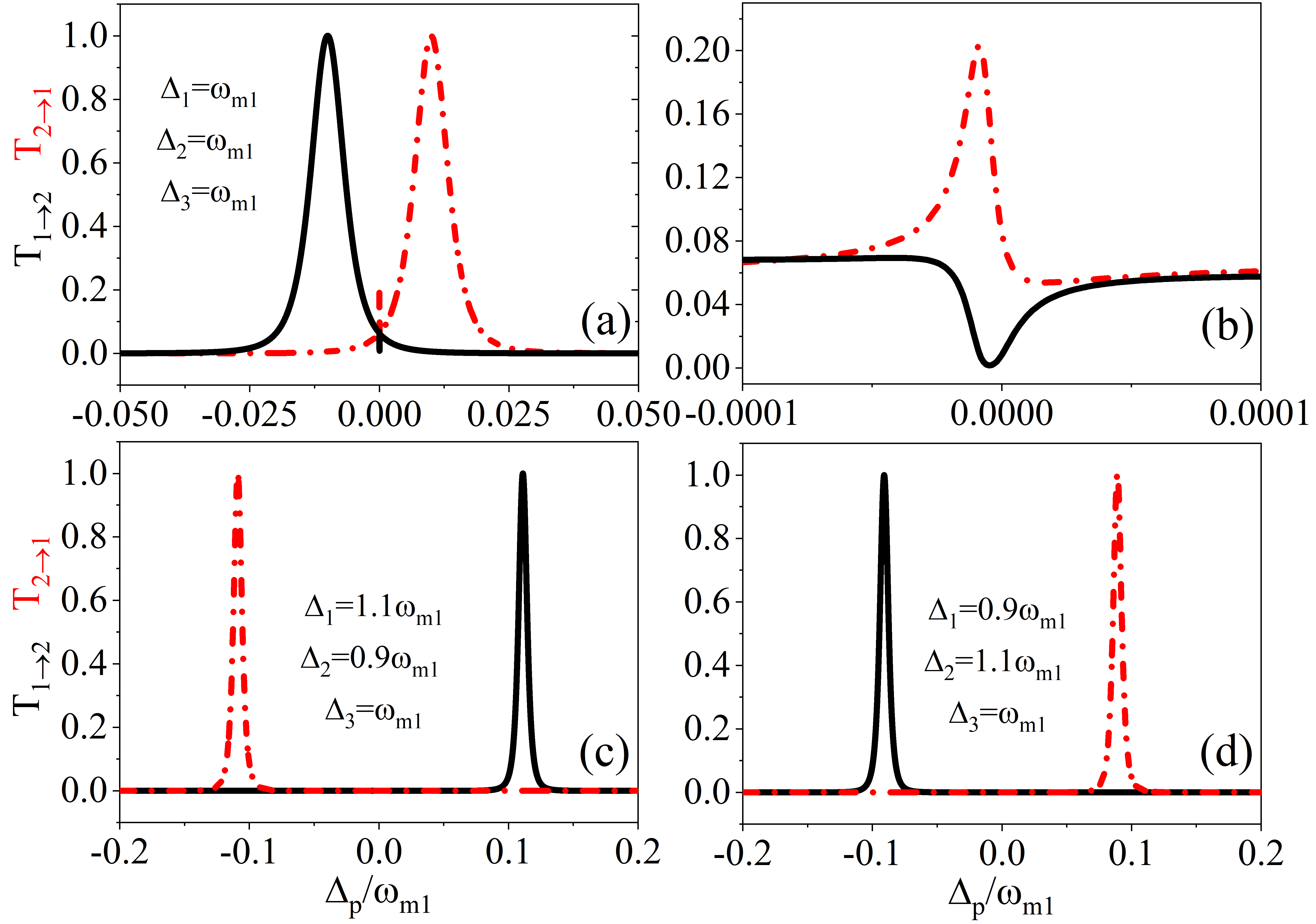
Figure 2: Transmission intensities T_2→1 (red dash-dot curves) and T_1→2 (black solid curves) as a function of the probe-drive field detuning $\Delta_{p}$ under different values of the effective cavity detunings: (a) the same values of effective cavity detunings $\Delta_{1}=\Delta_{2}=\Delta_{3}=\omega_{m1}$, (b) the inset for a short frequency range showing the smaller dip and peak of intensity profile near the origin of (a), (c) $\Delta_{1}=1.1\omega_{m1}$, $\Delta_{2}=0.9\omega_{m1}$, $\Delta_{3}=\omega_{m1}$, and (d) $\Delta_{1}=0.9\omega_{m1}$, $\Delta_{2}=1.1\omega_{m1}$, $\Delta_{3}=\omega_{m1}$. The general parameters are given as $\omega_{m1}/2\pi=\omega_{m2}/2\pi=12.6$ GHz, $\kappa_{1}/2\pi=\kappa_{2}/2\pi=\kappa_{3}/2\pi=73$ MHz, $\gamma_{1}/2\pi=\gamma_{2}/2\pi=88$ kHz, $\Delta_{a1}/2\pi=79.96$ GHz, $\Delta_{a2}/2\pi=78.38$ GHz, $\Delta_{a3}/2\pi=84.71$ GHz, $O_{m1}/2\pi=O_{m2}/2\pi=O_{m31}/2\pi=O_{m32}/2\pi=1.5$ MHz, $\textit{L}_{i}=\textit{L}_{3i}=5.19$ mm ($i=1,2$), $m_{\text{eff},j}=20\leavevmode\nobreak\ \upmu$g ($j=1,2$), $\Phi_{d1}=\Phi_{d2}=\Phi_{p1}=\Phi_{p2}=0$, $\Omega_{d1}=\Omega_{d2}=2\omega_{m1}$, and $\Omega_{p1}=\Omega_{p2}=0.2\omega_{m1}$.

In this section, we will numerically investigate the non-reciprocal behavior of the output signals using the COS scheme with two signal exchange ports. The vital role responsible for this phenomenon is played by the optomechanical interactions between the cavity photons and their respective NMRs’ phonons. It is worth noting that we have considered different (unequal) values for the three cavity detunings ($\Delta_{a1},\leavevmode\nobreak\ \Delta_{a2}$ and $\Delta_{a3}$) which disregards or eliminates the possibility of photon hopping from one into another cavity. For numerical simulations, we consider the practically realizable parameters from a recent experimental work whose values are given as ⁵¹ $\omega_{m1}/2\pi=\omega_{m2}/2\pi=12.6$ GHz, $\kappa_{1}/2\pi=\kappa_{2}/2\pi=\kappa_{3}/2\pi=73$ MHz, $\gamma_{1}/2\pi=\gamma_{2}/2\pi=88$ kHz, $O_{m1}/2\pi=O_{m2}/2\pi=O_{m31}/2\pi=O_{m32}/2\pi=1.5$ MHz, $\Delta_{a1}/2\pi=79.96$ GHz, $\Delta_{a2}/2\pi=78.38$ GHz, $\Delta_{a3}/2\pi=84.71$ GHz, $L_{i}=L_{3i}=5.19$ mm ($i=1,2,$), $m_{\text{eff},j}=20\leavevmode\nobreak\ \upmu$g ($j=1,2$), $\Phi_{d1}=\Phi_{d2}=\Phi_{p1}=\Phi_{p2}=0$, $\Omega_{d1}=\Omega_{d2}=2\omega_{m1}$, and $\Omega_{p1}=\Omega_{p2}=0.2\omega_{m1}$. Our proposed COS can offer an excellent control and manipulation ability to the non-reciprocal transmission. This proposal could be very critical in the quantum information processing, optical sensors, optical switches, isolators, full-duplex signal transmission and upcoming quantum nanotechnologies.

3.1 Tuning $\Delta_{1}$ and $\Delta_{2}$ to control non-reciprocity

The non-reciprocal phenomenon discussed here is based on the interference effect at near resonance conditions. The effective cavity detunings $\Delta_{i}$ ( $i=1,2$) play a basic role in controlling the signal transmission. A slight change in the values of $\Delta_{i}$ from the resonance value brings in a perfect non-reciprocal transmission around the origin as shown in Figure 2. First, we choose the values of effective cavity detunings to be at exact resonance, that is, $\Delta_{1}=\Delta_{2}=\Delta_{3}=\omega_{m1}$. Figure 2(a) reveals the corresponding result showing the non-reciprocal behavior of signal at ports 1 and 2 plotted by red and black curves, respectively. Both the curves are close to each other on the frequency axis separated by a small spike-like pattern that shows non-reciprocity of signal curves at their extremes. The spike-like curve is enlarged to have a clear picture for better understanding as shown in Figure 2b. The non-reciprocal behavior of signal inside the cavity setup happens owing to the quantum interference phenomenon between the fields in the optomechanical system. Now, by choosing the values $\Delta_{1}=1.1\omega_{m1}$ and $\Delta_{2}=0.9\omega_{m1}$, a perfect blockade of the probe signal T_1→2 and transmission T_2→1 close to $\Delta_{p}=\text{-}0.1\omega_{m1}$ (where the peak lies) on the frequency axis is achieved as depicted by the red curve shown in Figure 2c. Likewise, near $\Delta_{p}=0.1\omega_{m1}$ on the positive frequency axis away from the origin, scenario changes and the signal transfer T_1→2 is permitted while T_2→1 is completely blocked. To fully uncover the contribution of $\Delta_{i}$ to the non-reciprocity phenomenon, the values are chosen to be $\Delta_{1}=0.9\omega_{m1}$ and $\Delta_{2}=1.1\omega_{m1}$, so the transmission curve positions for both T_1→2 and T_2→1 on the frequency axis are switched oppositely to the previous case [see Figure 2c] and shift towards the origin as shown in Figure 2d. In both sub Figures mentioned above, the probe-field transfer via either port occurs because of constructive interference between the probe field-induced cavity field and the NMRs’ excitations (resonance frequencies), while the transmission blockade comes into play due to the destructive interference happening at the near-resonant conditions, and thus no probe signal is received at the output port. There is no signal transfer seen at either port for the frequencies other than mentioned above. Moreover, these interference patterns depend on the cavity detunings, since the radiation pressure varies with the change in $\Delta_{i}$ value which ultimately is accountable for breaking the time reversal symmetry and we obtain the non-reciprocal transmission. Hence, by tuning the effective cavity detunings as near-resonant with the NMRs’ excitations, the non-reciprocal output signal transfer via output ports can observed at a certain frequency range by using our proposed setup. The above discussion manifests non-reciprocity when the effective cavity detunings are slightly off-resonant with the mechanical excitations, and at exact resonance case ($\Delta_{i}=\omega_{m1}$) the signal non-reciprocal behavior is enhanced on account of increasing linewidth of the transmission curves. Hence the effective cavity detuning can be used to flexibly control the bidirectional output-signal transfer at either port as demanded.

3.2 Influence of optomechanical couplings on signal transmission

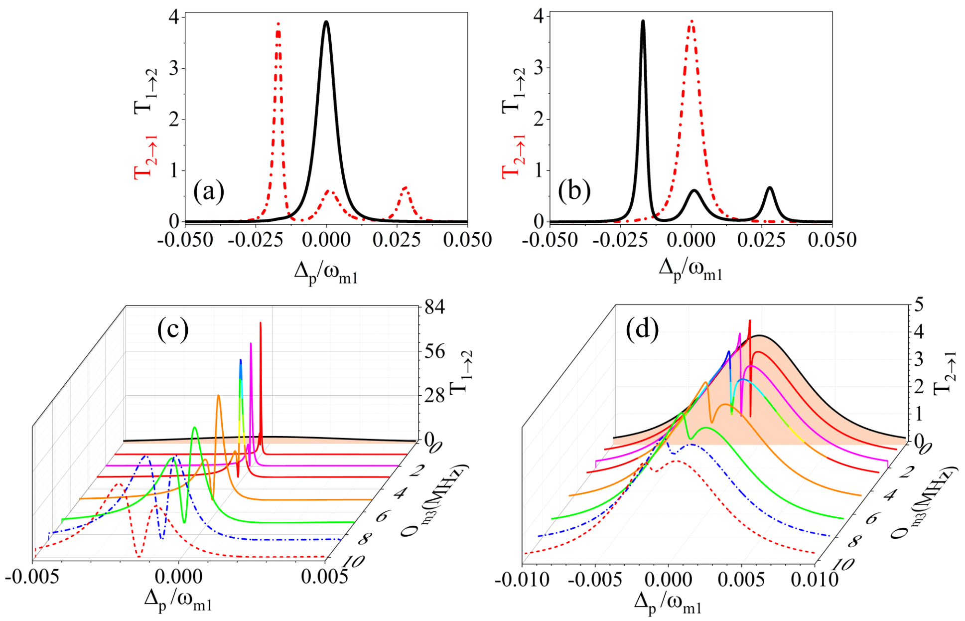
Figure 3: (Color online) (a) (b) Transmission intensities T_2→1 (red dash-dot curves) and T_1→2 (black solid curves) as a function of the probe-drive field detuning $\Delta_{p}$ under different values of optomechanical coupling strengths $O_{m1}$, $O_{m2}$, $O_{m31}$ and $O_{m32}$: (a) $O_{m1}/2\pi=1$ MHz, $O_{m2}/2\pi=60$ MHz, $O_{m31}/2\pi=O_{m32}/2\pi=O_{m3}/2\pi=48.5$ MHz, (b) $O_{m1}/2\pi=60$ MHz, $O_{m2}/2\pi=1$ MHz, $O_{m31}/2\pi=O_{m32}/2\pi=O_{m3}/2\pi=48.5$ MHz. (c)(d) The waterfall plots of transmission intensities T_1→2 and T_2→1 as a function of probe-drive field detuning $\Delta_{p}$ and $O_{m3}$ . The optomechanical couplings for (c), (d) are $O_{m1}/2\pi=1$ MHz, $O_{m2}/2\pi=60$ MHz. The general parameters are given as $\Delta_{a1}/2\pi=79.168$ GHz, $\Delta_{a2}/2\pi=79.160$ GHz, $\Delta_{a3}/2\pi=79.96$ GHz. Other values are same as mentioned in Figure 2a.

In cavity optomechanics, the optomechanical coupling strength between the intra-cavity photons and the NMR (which results from the radiation pressure of cavity photons on the NMR) plays a key role in inducing the nonlinearity into the cavity optomechanical system. Here we study the influence of optomechanical coupling strength in inducing and controlling the bidirectional non-reciprocal response of the output probe fields across two available routes (ports). Unlike the Faraday’s effect in magneto-optical materials that makes the time-reversal symmetry breaking happen, ⁹ the non-reciprocity in our proposed system arises due to the asymmetric radiation pressure of cavity photons on the NMRs when the optomechanical couplings are unequal. The interaction between cavity fields and mechanical oscillations forms a five-mode chain, i.e., $a_{1}\leftrightarrow b_{1}\leftrightarrow a_{3}\leftrightarrow b_{2}\leftrightarrow a_{2}$, thus operating in a closed loop pattern that posses quantum interference between the optical modes and mechanical excitations, and hence relying on constructive/destructive interference the flow/blockade of signal transfer becomes possible. The cavity mode $a_{3}$ in the middle (between NMRs) maintains a connection between the two mechanical modes and its optomechanical coupling strength plays crucial role regarding the behavior of signal at output ports. When the value of optomechanical interaction between cavity $a_{1}$ and NMR₁ is $O_{m1}=1$ MHz and relatively higher for cavity $a_{2}$ , that is, $O_{m2}=60$ MHz, it exhibits the optical signal transfer at port 1 without any restriction around the origin (shown by red dot-dashed peak), whereas in the same frequency range, the transmission of signal T_1→2 at port 2 is almost blocked as shown by the black solid curve depicted in Figure 3a.The physical picture for non-reciprocity comes from quantum interference among optical and mechanical modes in a similar fashion to the loop coupling of fields explained in Ref. ³⁷. The non-reciprocity comes into play when the radiation pressure on the mechanical resonators is not even. In that case, the constructive interference among the mechanical excitations and optical driven fields leads to a high efficiency amplified output signal, whereas destructive interference brings the output down to zero. In the case, the radiation pressure remains same for all optomechanical couplings, no breaking of time reversal symmetry happens and thus signal behavior is completely reciprocal. Due to destructive interference, i.e., in case of $O_{m1}<O_{m2}$, the signal is blocked in the T_1→2 direction, whilst at the same time, the signal transit becomes viable due to the reverse effect, that is, constructive interference around the resonance point. The constructive/destructive interference effect between the mechanical excitations and probe-induced cavity field happens here due to the asymmetry of the radiation pressure on the NMRs, ⁵² which comes into play because of the changes in cavity lengths since the optomechanical couplings depend on the cavity lengths, i.e., $O_{mi}=\frac{\omega_{ai}}{L_{i}}\sqrt{\frac{\hbar}{m_{\text{eff},i}\omega_{mi}}}$ and $O_{3i}=\frac{\omega_{a3}}{L_{3i}}\sqrt{\frac{\hbar}{m_{\text{eff},i}\omega_{mi}}}$ ($i=1,2$), ⁴² where $L_{i}$ and $L_{3i}$ are the cavity lengths and $m_{\text{eff},i}$ is the effective mass of NMR. The scenario changes completely when the optomechanical couplings satisfy $O_{m2}>O_{m1}$ as given in Figure 3b. When $O_{m1}=60$ MHz and $O_{m2}=1$ MHz, signal transmission from port 1 to 2 can be realized having no output at port 1 around the origin. An amplification of output signal transmission can be seen which comes into play because of the constructive interference between different transmission paths, i.e., $a_{1}\leftrightarrow b_{1}\leftrightarrow a_{3}\leftrightarrow b_{2}\leftrightarrow a_{2}$ and $a_{2}\leftrightarrow b_{2}\leftrightarrow a_{3}\leftrightarrow b_{1}\leftrightarrow a_{1}$. ⁵³ The amplification of output field has been reported in cavity optomechanical systems multiple times using different cavity setups. ^{54, 31, 55, 56, 57} However, when the optomechanical couplings become equal/same, that is, $O_{m1}=O_{m2}$, the signal transmission behavior turns completely to reciprocal as a result of symmetric radiation pressure on both the NMRs. For example, when $O_{m1}=O_{m2}$, the signal is allowed to pass through both output ports by the same amount at/around the origin on the frequency axis (not shown here) which is reciprocal in nature.

In our proposed setup, the optomechanical couplings, i.e., $O_{m31}=O_{m32}=O_{m3}$ associated with cavity mode $a_{3}$ and NMRs are of great interest in realizing the conversion of reciprocal to non-reciprocal behavior of output fields. Non-reciprocity is valid if $O_{m3}$ is non-zero under the condition $O_{m1}\neq O_{m2}$. In the case, the coupling $O_{m3}$ goes down to zero, the non-reciprocity is lost, and the system is left with complete reciprocal signal transmission at output ports regardless of the values (higher or lower) assigned to couplings $O_{m1}$ and $O_{m2}$ as shown in Figure 3c,d. Now, to see the output signal’s nature turning from reciprocal to non-reciprocal, the system in this case rely on optomechanical coupling $O_{m3}$ value. Figure 3c,d show reciprocal signal transfer at both ports 2 and 1, respectively, having their maxima at the origin when $O_{m31}=O_{m32}=O_{m3}=0$ as expressed by black curves. The interference pattern is effectively modified as the coupling $O_{m3}$ step up to non-zero value, and thus the reciprocal nature of output signal at both ports is gradually transformed into non-reciprocal. The signal transfer T_1→2 becomes dominantly amplified and its curve splits into two by further increasing the value of $O_{m3}$ thus gaining Fano-like steep peaks, while the curve for T_2→1 also acquires a Fano-shaped profile keeping almost the same intensity. By further increasing the value of $O_{m3}$ (8.5 MHz), the Fano-profiled asymmetric peaks of T_1→2 become symmetric and skid away from the origin on frequency axis. On the other hand, the signal transfer T_2→1 stays on the origin and two small peaks smoothly converge to single peak. Beyond 8.5 MHz of $O_{m3}$ value, the transmission T_1→2 curve profile at port 2 changes again from symmetric to asymmetric with its line-width being broadened thus showing effectively the output signal transfer away from origin. The output signal transmission T_2→1 at port 1 owns the same curve pattern with single peak at constant intensity as shown in Figure  3(d). From Figure 3c,d, it is obvious that by increasing the value of $O_{m3}$ the signal transfer at both ports gradually convert from reciprocal to non-reciprocal.

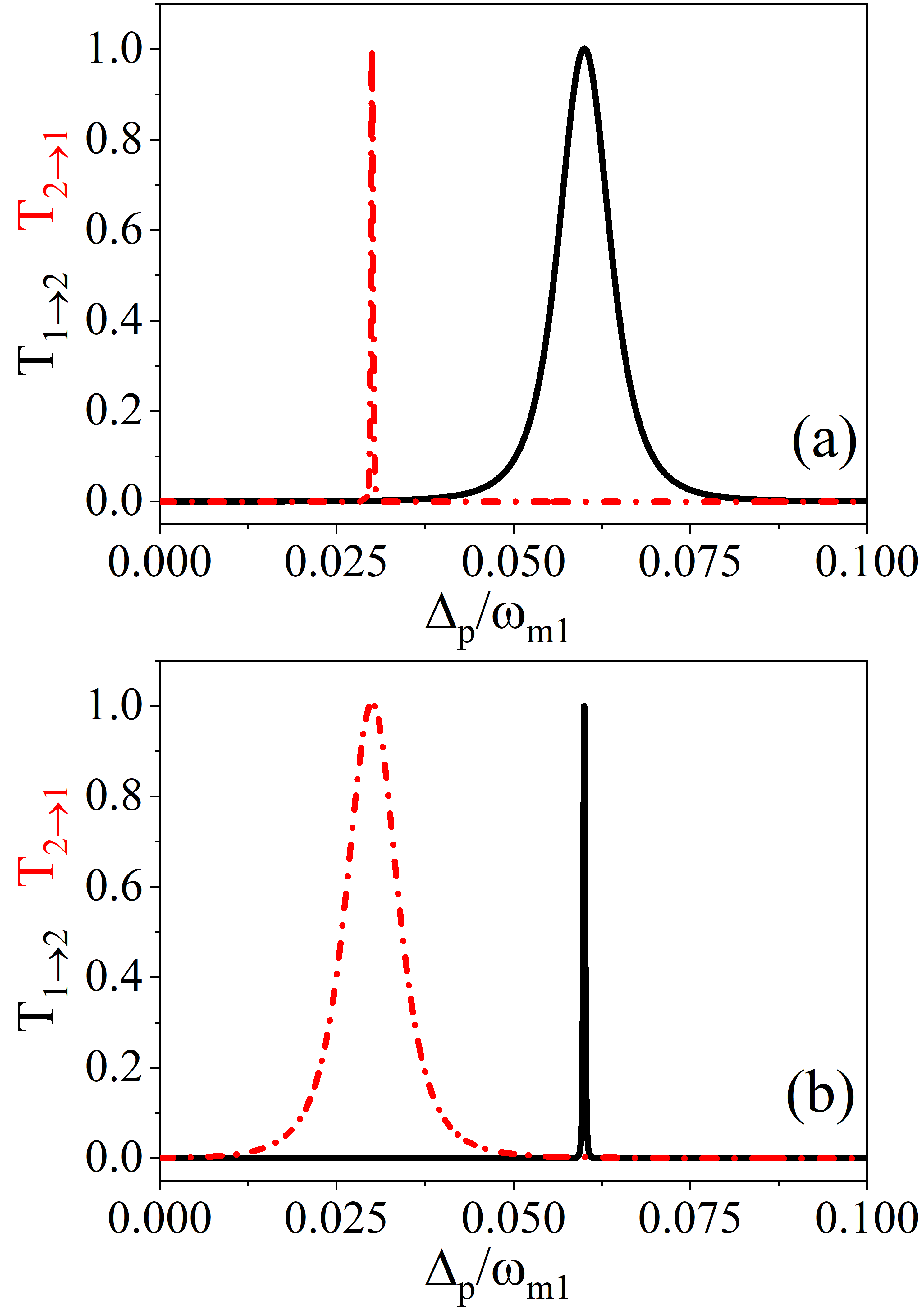
Figure 4: Probe transmission intensities T_2→1 (red dash-dot) and T_1→2 (black solid) as a function of probe-drive field detuning under different values of cavity decay rates: (a) $\kappa_{1}/2\pi=83$ MHz, $\kappa_{2}/2\pi=3$ MHz, $\kappa_{3}/2\pi=73$ MHz, and (b) $\kappa_{1}/2\pi=3$ MHz, $\kappa_{2}/2\pi=83$ MHz, $\kappa_{3}/2\pi=73$ MHz. The general parameters are given as, $\Delta_{1}=\Delta_{2}=\Delta_{3}=\omega_{m1}$, whereas other parameter values are same as in Figure 2a

.

Thus, the above discussion justifies the fact that signal transmission at either port can be controlled flexibly from reciprocal to non-reciprocal and vice versa by changing the optomechanical couplings.

3.3 Effect of cavity decay rates on the signal flow

Every COS inherits intrinsic photons dissipation to external bath (cavity decay rate) that depends on the quality factor $Q$ of the end mirrors. Similarly, in our proposed cavity setup, the role of cavity decay rate $\kappa_{i}$ is inevitable and thus affects the bidirectional signal transfer. As the transmission happens via left and right ports, we consider changes in the cavity decay rates associated with cavities $a_{1}$ and $a_{2}$ only. In Figure 4a, when the cavity decay rates have $\kappa_{1}>\kappa_{2}$, the system allows the output probe signal from port 1 to port 2 with maximum value ( equal to 1) of T_1→2 as shown by black colored peak with large linewidth, but blocks it in the opposite direction, i.e., from port 2 to port 1 with transmission value of T_2→1 equal to zero. The above relation between two decay rates insinuate the razing of photons in cavity $a_{1}$ as compared to cavity $a_{2}$ which eventually results in suppressing of optical signals through cavity $a_{1}$ and thus to port 1. However, the signal is transferred efficiently in reverse direction T_1→2. The larger amount of $\kappa_{1}$ is responsible for lowering the photon number and thus, the optomechanical coupling in cavity $a_{1}$ as compared to $\kappa_{2}$ value which results in comparatively larger optomechanical coupling in cavity $a_{2}$ and thus time reversal symmetry breaking happens that accounts for the non-reciprocal transmission. Due to the quantum interference mentioned in the above paragraphs, an ultra-thin peak can be achieved for T_2→1 at a different frequency range where transmission in the opposite direction is zero thus showing the non-reciprocal behavior. Figure 4b reveals the case for signal transfer when $\kappa_{1}<\kappa_{2}$, so the converse happens that provokes the signal transmission from port 2 to 1 T_2→1 and suppresses it in the reverse direction, that is, T_1→2. Hence, the cavity with larger value of $\kappa$ blocks signal transfer at its respective port coming from the other one, while cavity with lower decay rate supports signal transmission at the same port. Thus, non-reciprocity can be observed by considering the cavity decay rate values where the signal transfer behavior can be manipulated.

3.4 Effect of probe and drive phases on signal flow

Figure 5: Dependence of transmission intensities T_2→1 (red dash-dot) and T_1→2 (black solid) on the probe-drive field detuning $\Delta_{p}$ when (a) probe phases $\Phi_{p1}=\Phi_{p2}=0$, (b) $\Phi_{p1}=\Phi_{p2}=2\pi/3$, (c) $\Phi_{p1}=-2\pi/3,\leavevmode\nobreak\ \Phi_{p2}=2\pi/3$. The general parameters are given as $\Delta_{1}=\Delta_{2}=\Delta_{3}=\omega_{m1}$, and other parameter values are same as in Figure 2(a).

Figure 6: Density plot for the transmission intensities (a) T_1→2 and (b) T_2→1 against the probe detuning $\Delta_{p}$ and the relative phase $\phi_{\text{rel}}$. The general parameter values are given as $\Delta_{1}=\Delta_{2}=\Delta_{3}=\omega_{m1}$. Other values are same as in Figure 2a

.

Generally, the phases of interacting fields play an important role in the interference phenomenon. Here we explain the significance of external probe and drive field phases that enables the cavity system to behave non-reciprocal for signal transmission at either port. These phase changes from both inputs are analogous to the synthetic magnetic field that is responsible for breaking time reversal symmetry and can be used as bidirectional non-reciprocal signal transport device. ⁵⁸ First, we suppose that the incoming external probe fields from either port have no phase change, that is, $\Phi_{p1}=\Phi_{p2}=0$. We report a complete non-reciprocal signal transfer via both ports with single transmission peak (black and red) at separate places on the frequency axis as shown in Figure 5a. Now, as the phases of probe fields are changed to $\Phi_{p1}=\Phi_{p2}=2\pi/3$, we still obtain non-reciprocal transmission curves with Fano-like profile shown by Figure 5b. Since the signs of both the probe phases are positive, the curves attain the same profile at different positions on the probe detuning axis. As we change the sign of probe phase, i.e., $\Phi_{p1}=-2\pi/3$ and $\Phi_{p2}=2\pi/3$, the transmission T_1→2 is shifted to the right side of origin having the same Fano-like shape as depicted by Figure 5b. The output signal transfer T_2→1 shifts to the left of resonance position and reverses its direction due to the change in sign of probe phase as shown in Figure 5c. The direction of non-reciprocal transmission completely reverses when the phases signs are changed, that is, $\Phi_{p1}=2\pi/3$ and $\Phi_{p2}=-2\pi/3$ not presented here in figure. The same result given in Figure 5c can be achieved for the phase changes equal to $\Phi_{p1}=\pi/3$ and $\Phi_{p2}=-\pi/3$.

Continuing the explanation of phases’ role in controlling the behavior of signal transmission, we check the sensitivity of system to external fields phase on the non-reciprocal signal transfer. Since there are four electromagnetic fields (two drive and two probe fields) with corresponding phases $\Phi_{p1}$, $\Phi_{p2}$, $\Phi_{d1}$ and $\Phi_{d2}$ interacting with the cavity via two ports, it is vital to investigate the role of collective phase [also known as relative phase] in controlling the behavior of signal transferred at either port. The collective/relative phase can be expressed as $\phi_{\text{rel}}=(\Phi_{p1}+\Phi_{p2})-(\Phi_{d1}+\Phi_{d2})$, ^{59, 60} and could be conveniently determined by recalculating Equation (17) and (18). Referring to Figure 6, a density graph for the signal flow at the two ports has been plotted. Here we check the sensitivity of system to the relative phase $\phi_{\text{rel}}$ regarding the non-reciprocal signal transfer. Figure 6a illustrates the transmission of signal from port 1 to 2 while Figure 6b reveals the flow in reverse direction, that is, from port 2 to 1. By considering the relative phase, signal transmission T_1→2 and T_2→1 along the two opposite routes have a complete non-reciprocal nature which is depicted by the contours in Figure 6a and 6b, respectively. The contours demonstrate that when the relative phase is in the regions around $\phi_{\text{rel}}=-2\leavevmode\nobreak\ \text{to}\leavevmode\nobreak\ 0$ and $\phi_{\text{rel}}=-1\leavevmode\nobreak\ \text{to beyond}\leavevmode\nobreak\ 2$ at the left frequency band of probe detuning, maximum signal transfer T_1→2 is achieved at its corresponding port 2, whereas the output signal T_2→1 at port 1 is fully suppressed at that bandwidth of detuning frequency, thus, revealing its sensitivity upon the relative phase. The same explanation goes for the upper half contour where signal intensity lies. However, the signal transmission T_2→1 at port 1 is maximum for the similar range of relative phase mentioned above on the right of resonance point on frequency axis, but there is no signal flowing in the opposite direction which again justifies the non-reciprocal behavior of output signal transfer. As mentioned in the discussion corresponding to Figure 5, the non-reciprocal behavior of signal transmission taking place here is due to the quantum interference since a change in the relative phase of the fields may alter the interference pattern, thus resulting in the non-reciprocity due to the time reversal symmetry breaking. The signal from both ports also overlap in a certain range of relative phase values, i.e., $\phi_{\text{rel}}=0.75\leavevmode\nobreak\ \text{to almost}\leavevmode\nobreak\ 1$ hence revealing the reciprocal nature of output signals. The above explanation suggests that the output signal’s nature strongly depends on the relative phase which can be switched from reciprocal to non-reciprocal and vice versa. Thus, by changing the probe and/or drive field and relative phase we can flexibly control the bi-directional non-reciprocal nature of the output signal at either port.

From the above description, it is clear that our proposed COS setup is phase-sensitive and non-reciprocal signal transfer is possible by changing the phases of external probe fields and drive fields.

4 Summary

We have theoretically investigated the non-reciprocal behavior of the output probe fields through a bidirectional multi-mode COS being driven by external classical fields. A perfect non-reciprocal transmission of signal due to the breaking of time reversal symmetry has been revealed at the effective cavity detunings $\Delta_{1}$, $\Delta_{2}$ close to mechanical frequency, and a full duplex transmission is tunable by adjusting the values of $\Delta_{1}$ and $\Delta_{2}$. By modifying and flexibly controlling the optomechanical couplings, signal transfer has been blocked from passing via one port (terminal) and passed on through other around resonance conditions. Additionally, the nature of output signal has been realized to transform from reciprocal to non-reciprocal by smoothly tuning the optomechanical coupling values. The non-reciprocal signal transfer is also influenced by tuning the cavity decay rates, which are the intrinsic parameters that cannot be omitted. Interestingly, the phase changes and the relative phase associated with input probe and drive fields from either port have crucial impact on the signal transport and the transmission from reciprocal to non-reciprocal and vice versa. This scheme suggested may be practically feasible in laboratory since it is based on cavity setup that has already been realized in experiments and is rooted on realistic system parameters. We hope that the proposed theoretical model could be the right route for experimentalists to explore a new and efficient way for manufacturing non-reciprocal devices like routers, optical isolators, sensors, light diodes, and full duplex signal transmitters and transducers.

Conflict of interest

The authors declare no conflict of interest.

Data Availability Statement

The data that support the findings of this study are available from the corresponding author upon reasonable request.

References

- [1] D. L. Sounas, A. Al, Nat. Photonics, 2017 11 774.
-
[2]
H. A. Lorentz, Amsterdammer Akademie der
Wetenschappen, 1896,
4 176; https://ci.nii.ac.jp/naid
/10018471922/en/ - [3] M. Levy, J. Opt. Soc. Am. B 2005, 22, 254.
- [4] T. R. Zaman, X. Guo, R. J. Ram, Appl. Phys. Lett. 2007, 90, 023514.
- [5] H. Dotsch, N. Bahlmann, O. Zhuromskyy, M. Hammer, L. Wilkens, R. Gerhardt, P. Hertel, A. F. Popkov, J. Opt. Soc. Am. B 2005, 22 240.
- [6] Z. Wang, Y. Chong, J. D. Joannopoulos, M. Soljai, Nature (London), 2009, 461, 772.
- [7] A. B. Khanikaev, S. H. Mousavi, G. Shvets, Y. S. Kivshar, Phys. Rev. Lett. 2010, 105, 126804.
- [8] L. Bi, J. Hu, P. Jiang, D. H. Kim, G. F. Dionne, L. C. Kimerling, C. A. Ross, Nat. Photonics, 2011, 5 758.
- [9] J. Y. Chin, T. Steinle, T. Wehlus, D. Dregely, T. Weiss, V. I. Belotelov, B. Stritzker, H. Giessen, Nat. Commun. 2013, 4, 1599.
- [10] D. Dai, J. Bauters, J. E. Bowers, Light Sci. Appl. 2012, 1, e1.
- [11] N. A. Estep, D. L. Sounas, J. Soric, A. Al, Nat. Phys. 2014, 10, 923.
- [12] J. Kerckhoff, K. Lalumire, B. J. Chapman, A. Blais, K. W. Lehnert, Phys. Rev. Appl. 2015, 4, 034002.
- [13] L. Ranzani, J. Aumentado, New J. Phys. 2014, 16, 103027.
- [14] T. C. White, J. Y. Mutus, I.-C. Hoi, R. Barends, B. Campbell, Y. Chen, Z. Chen, B. Chiaro, A. Dunsworth, E. Jeffrey, J. Kelly, A. Megrant, C. Neill, P. J. J. O’Malley, P. Roushan, D. Sank, A. Vainsencher, J. Wenner, S. Chaudhuri J. Gao, J. M. Martinis, Appl. Phys. Lett. 2015, 106, 242601.
- [15] C. Macklin, K. O’Brien, D. Hover, M. E. Schwartz, V. Bolkhovsky, X. Zhang, W. D. Oliver, I. Siddiqi, Science, 2015, 350, 307.
- [16] S. Hua, J. Wen, X. Jiang, Q. Hua, L. Jiang, M. Xiao, Nat. Commun. 2016, 7, 13657.
- [17] M. Hafezi, P. Rabl, Opt. Express 2012, 20, 7672.
- [18] Z. Shen, Y.-L. Zhang, Y. Chen, C.-L. Zou, Y.-F. Xiao, X.-B. Zou, F.-W. Sun, G.-C. Guo, C.-H. Dong, Nat. Photonics, 2016, 10 657.
- [19] P. Meystre, Ann. Phys. (Berlin) 2013, 525 No. 3, 215.
- [20] S.-S. Chen, S.-S. Meng, Hong Deng, G.-J. Yang, Ann. Phys. (Berlin) 2020, 533, 2000343; https://doi.org/10.1002/andp.202000343
- [21] Z. Shen, Y.-L. Zhang, Y. Chen, F.-W. Sun, X.-B. Zou, G.-C. Guo, C.-L. Zou, C.-H. Dong, Nat. Commun. 2018, 9, 1797.
- [22] S. J. M. Habraken, K. Stannigel, M. D. Lukin, P.Zoller, New J. Phys. 2012, 14, 115004.
- [23] X.-W. Xu, Y. Li, Phys. Rev. A 2015, 91, 053854.
- [24] B.-Y. Zhou, G.-X. Li, Phys. Rev. A 2016, 94, 033809.
- [25] O. Cernotk, C. Genes, A. Dantan, Quantum Sci. Technol. 2019, 4, 024002.
- [26] H. Tan, W. Deng, Q. Wu, G. Li, Phys. Rev. A 2017, 95, 053842.
- [27] Ziauddin, M. U. Rahman, I. Ahmad, S. Qamar, Euro phys. Lett. 2017, 120, 24001; https://iopscience.iop.org/article/10.1209/0295-5075/120/24001.
- [28] M. Ullah, A. Abbas, J. Jing, L.-G. Wang, Phys. Rev. A 2019, 100, 063833.
- [29] K. Qu, G. S. Agarwal, Phys. Rev. A 2013, 87, 063813.
- [30] T. Kipf, G. S. Agarwal, Phys. Rev. A 2014, 90, 053808.
- [31] L.-G. Si, H. Xiong, M. S. Zubairy, Y. Wu, Phys. Rev. A 2017, 95, 033803.
- [32] V. Bergholm, W. Wieczorek, T.-S. Herbrggen, M. Keyl, Quantum Sci. Technol. 2019, 4, 034001.
- [33] N. Kralj, M. Rossi, S. Zippilli, R. Natali, A. Borrielli, G. Pandraud, E. Serra, G. D. Giuseppe, D. Vitali, Quantum Sci. Technol. 2017, 2, 034014.
- [34] G. A. Peterson, F. Lecocq, K. Cicak, R. W. Simmonds, J. Aumentado, J. D. Teufel, Phys. Rev. X 2017, 7, 031001.
- [35] N. R. Bernier, L. D. Tth, A. Koottandavida, M. A. Ioannou, D. Malz, A. Nunnenkamp, A. K. Feofanov, T. J. Kippenberg, Nat. Commun. 2017, 8, 604.
- [36] S. Barzanjeh, M. Wulf, M. Peruzzo, M. Kalaee, P. B. Dieterle, O. Painter, J. M. Fink, Nat. Commun. 2017, 8, 953.
- [37] X.-W. Xu, Y. Li, A.-X. Chen, Y.-X. Liu, Phys. Rev. A 2016, 93, 023827.
- [38] L. Tian, Z. Li, Phys. Rev. A 2017, 96, 013808.
- [39] L. M. de Lpinay, C. F. Ockeloen-Korppi, D. Malz, M. A. Sillanp, Phys. Rev. Lett. 2020, 125, 023603.
- [40] S. Liu, B. Liu, J. Wang, L. Zhao, W.-X. Yang, J. Appl. Phys. 2021, 129, 084504.
- [41] G. S. Agarwal, S. Huang, Phys. Rev. A 2010, 81, 041803(R).
- [42] M. J. Akram, M. M. Khan, F. Saif, Phys. Rev. A 2015, 92, 023846.
- [43] Q. He, F. Badshah, L. Li, L. Wang, S.-L. Su, E. Liang, Ann. Phys. (Berlin) 2021, 533(5) 2000612; https://doi.org/10.1002/andp.202000612.
- [44] D. Vitali, S. Gigan, A. Ferreira, H. R. Bhm, P. Tombesi, A. Guerreiro, V. Vedral, A. Zeilinger, M. Aspelmeyer, Phys. Rev. Lett. 2007, 98, 030405.
- [45] S. Huang, G. S. Agarwal, New J. Phys. 2009, 11, 103044.
- [46] C.-L. Zou, X.-B. Zou, F.-W. Sun, Z.-F. Han, G.-C. Guo, Phys. Rev. A 2011, 84, 032317.
- [47] G. S. Agarwal, S. Huang, New J. Phys. 2014, 16, 033023.
- [48] D. F. Walls, G. J. Milburn, Quantum Optics, Springer-Verlag, Berlin 1994.
- [49] X. B. Yan, C. L. Cui, K. H. Gu, X. D. Tian, C. B. Fu, J. H. Wu, Opt. Express 2014, 22(5), 4886.
- [50] X.-W. Xu, L. N. Song, Q. Zheng, Z. H. Wang, Y. Li, Phys. Rev. A 2018, 98, 063845.
- [51] P. Kharel, G. I. Harris, E. A. Kittlaus, W. H. Renninger, N. T. Otterstrom, J. G. E. Harris, P. T. Rakich, Sci. Adv. 2019, 5, eaav0582.
- [52] S Manipatruni, J. T. Robinson, M. Lipson, Phys. Rev. Lett. 2009, 102, 213903.
- [53] L. Du, Y.-T. Chen, Wu J.-H. Wu, Y. Li, Opt. Express 2020, 28, 3647.
- [54] Y. L. Liu, R. Wu, J. Zhang, S. K. Ozdemir, L. Yang, F. Nori, Y. X. Liu, Phys. Rev. A 2017, 95(1), 013843.
- [55] Y. Li, Y. Huang, X. Zhang, L. Tian, Opt. Express 2017, 25, 18907.
- [56] C. Jiang, B. Ji, Y. Cui, F. Zuo, J. Shi, G. Chen, Opt. Express 2018, 26, 15255.
- [57] W.-A. Li, G.-Y. Huang, Y. Chen, J. Opt. Soc. Am. B 2019, 36, 306.
- [58] F. Ruesink, J. P. Mathew, M. A. Miri, A. Al, E. Verhagen, Nat. Commun. 2018, 9, 1798.
- [59] M. Sahrai, H. Tajalli, K. T. Kapale, M. S. Zubairy, Phys. Rev. A 2004, 70, 023813.
- [60] L.-G. Wang, S. Qamar, S.-Y. Zhu, M. S. Zubairy, Phys. Rev. A 2008, 77, 033833.