A Tsallis-like effective exponential delay discounting model and its implications

Abstract

We propose an effective exponential model of delay discounting considering fluctuation in impulsivity. This model is seen to be dual to the two-parameter Tsallis model of delay discounting proposed by Takahashi in 2007 (Ref. takahashi1 ). We demonstrate that the parameters of the model can be related to the mean and the variance of impulsivity. Our findings provide an intuitive way to explore the origin of the Tsallis distribution in a social system.

Keywords: Tsallis statistics, delay discounting model, impulsivity fluctuation

I Introduction

Delay discounting is associated with the evolution of the value of a reward with delay to its receipt. For example, money of an amount $x$ received immediately is more ‘valuable’ than the amount received after a delay time $t$. However, when some features about a situation remain unspecified, uncertainties in decision arise and making a choice becomes more difficult. One such example is choosing between USD 50 right now and USD 70 in a year. In this case, one has to choose between smaller-sooner rewards and larger-later rewards. One example of choosing a smaller-sooner reward is a student unprepared for an exam going to a party the night before the test. The immediate reward brought out of this action appears to be more desirable than a delayed reward (which may be of greater value in terms of career, earning and so on). Choosing the smaller-sooner reward is termed as an impulsive action by the behavioral analysts ikuk . This implies recognizing more distant rewards as of lesser value. For a variety of species, reward types and sample, the value of a reward is discounted over time mazur ; bdm ; lempert ; west ; cajueiro . However, there is more to the story.

In behavioral studies, the rationality of agents has long been a matter of discussion and debate kahneman . In the studies of discounting, rational behavior of an agent is characeterized by inter-temporal consistency which may be understood from the following example. Let us assume that two sets of a pair of options are given to participants. Options in set 1 are A1) USD 100 available after 365 days, and B1) USD 120 available after 372 days. Options in set 2 are A2) USD 100 available right now, and B2) USD 120 available after 7 days. Choices A1 and A2 are more impulsive than B1 and B2 respectively because these choices manifest a preference for smaller-sooner rewards. However, things become interesting when a participant is asked to choose one option from both sets during a single experiment. Many people may opt for the smaller-sooner reward in set 1, whereas for set 2 they settle in for a larger-later reward (despite the waiting time in both cases are 7 days). This inconsistency in degree of impulsivity is known as ‘irrationality’. However, if in both cases one takes impulsive decisions, that is still rational, and the same is true for those who consistently opt for larger-later rewards in both cases.

In the case of rational agents, the exponential model of delay discounting is seen to be appropriate. The exponential delay discounting model considers an exponential dependence of the subjective value of a reward on delay given by,

$$V(D)=V(0)\exp({-\kappa D}),$$ (1)

where $V(D)$ is the discounted value of a reward after a delay $D$, $V(0)>V(D)$ is the undiscounted value of the reward, and $\kappa$ is the impulsivity parameter.

Exponential model is related to the situation when the discount rate is constant over time. However, things change when this is not the case. In that case, the exponential model becomes unable to explain inter-temporal inconsistency described in a previous paragraph. Several other models like the hyperbolic model rachilinhyp have been proposed to consider this phenomenon in the behavioral studies. But, the hyperbolic model cannot differentiate between inconsistency and impulsivity. This is the reason why Takahashi takahashi1 proposed a delay discounting model based on the Tsallis $q$-exponential function which was also used by Cajueiro cajueiro in a study on inter-temporal choices.

Unlike the exponential model, the Tsallis model is described by two parameters, $q$ (also called the Tsallis $q$ parameter) and impulsivity $\kappa$. A fundamental approach involving the mathematical techniques of complex Hilbert space used in quantum mechanics has been taken by Yukalov and Sornette yukalov . By considering a time-dependent decay rate in the evolution of a ‘prospect set’, they obtain a power-law time discounting function which is similar to the Tsallis function. Hence the Tsallis function comes both as a necessity to describe the observed phenomenon and as a consequence of a very general mathematical ritual. Because of these reasons, the Tsallis $q$-exponential function (henceforth to be called the Tsallis function) has been used in many behavioral studies over the years takahashi2 ; takahashiqdt ; lempert ; fpsy1 ; fph1 ; ejmbe .

As indicated in one of them takahashi2 , the Tsallis function has its origin in physics. This function can be obtained from the Tsallis entropy, which is a generalization of the Boltzmann-Gibbs entropy. While maximization of the Boltzmann-Gibbs entropy gives rise to the exponential function, maximization of the Tsallis entropy yields a Tsallis $q$-exponential function. This approach of getting the Tsallis function may be termed as the ‘thermodynamic approach’ which is a standard procedure of obtaining the equilibrium (maximum entropy state, to be understood as the state with the maximum disorderliness) thermodynamic quantities in systems considered in physics.

However, in the present article, we do not consider the approach involving maximization in a social system (see for example cajueiro ). Here we rather try to examine why the Tsallis function may appear in a social system from a perspective that is different from the ones presented in takahashi2 ; yukalov . The approach taken by us is known as the so-called ‘super-statistics approach’ beck ; wilkprl which helps one build another intuitive understanding of the model. This approach is based on the fact that social and physical systems contain fluctuations. Let us take the example of the temperature of a room. Even though we say that the ‘room temperature’ is 30${}^{\text{o}}$C (say), this may not reflect the reality that the temperature in one corner of the room may be slightly below (say 29.8${}^{\text{o}}$C), and the other corner may be slightly above (say 31.2${}^{\text{o}}$C) than 30${}^{\text{o}}$. So, where does this number 30 come from? This may be the average temperature of the room. If, for example, we have $n_{1}$ different points in the room having temperature $T_{1}$, $n_{2}$ different points in the room having temperature $T_{2}$ and so on, the average temperature of the room is defined by $\left(n_{1}T_{1}+n_{2}T_{2}+....\right)/(n_{1}+n_{2}+...)$. In social systems too we encounter fluctuating quantities that follow some distributions, and the quantities like mean, variance become of our interest.

The novelty of the present work lies in the fact that from this simple consideration of a fluctuating system, the parameters used in the Tsallis model may be given some physical meaning. Although we do not deny that the Tsallis parameter (to be denoted as $q$) is already identified with the ‘measure of inconsistency’ cajueiro ; takahashi1 , our approach provides another intuitive way of looking at the model parameters. With this general consideration, we propose a model called the effective exponential model which contains a Tsallis function and has some correspondence with the existing Tsallis models.

The paper is organized in the following way. In the next section, we discuss the effective exponential model in detail. Section III contains a detailed discussion of our findings. Next, we summarize and conclude in Sec. IV.

II Description of the model and its application

II.1 Fluctuating impulsivity: how is it distributed?

We consider a social system in which impulsivity $\kappa$ is a positive, random variable. But we assume that we do not know anything about how they are distributed. In a typical statistical problem, we have a random variable whose distribution is unknown. In that case, the gamma distribution serves as the least-informative option hogg . Let us assume that the impulsivity distribution of a sample is given by the normalized (integrates to 1) gamma distribution,

$$f(\kappa)=\frac{1}{\Gamma\left(\frac{1}{q-1}\right)}\left\{\frac{1}{(q-1)\kappa_{0}}\right\}\left\{\frac{\kappa}{(q-1)\kappa_{0}}\right\}^{\frac{1}{q-1}-1}\exp\left(-\frac{\kappa}{(q-1)\kappa_{0}}\right),$$ (2)

where $q>1$ and $\kappa_{0}>0$ (so that $f(\kappa)$ is a positive real number) are two parameters, and the $\Gamma$ function is represented by the following integral when $q>1$,

$$\Gamma\left(\frac{1}{q-1}\right)=\int_{0}^{\infty}\exp(-x)x^{\frac{1}{q-1}-1}dx.$$ (3)

For different $q$ and $\kappa_{0}$ values the gamma distribution in Eq. (2) give rise to different shapes as can be seen in Figs. 2 and  2.

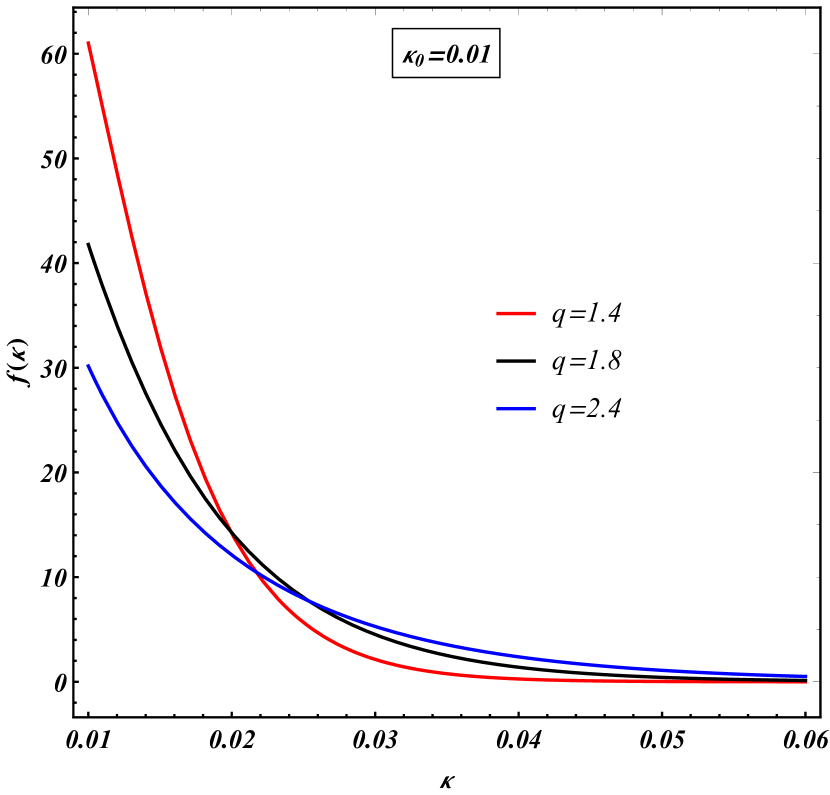
Figure 1: Gamma distributions for a fixed $\kappa_{0}$ and different $q$ values.

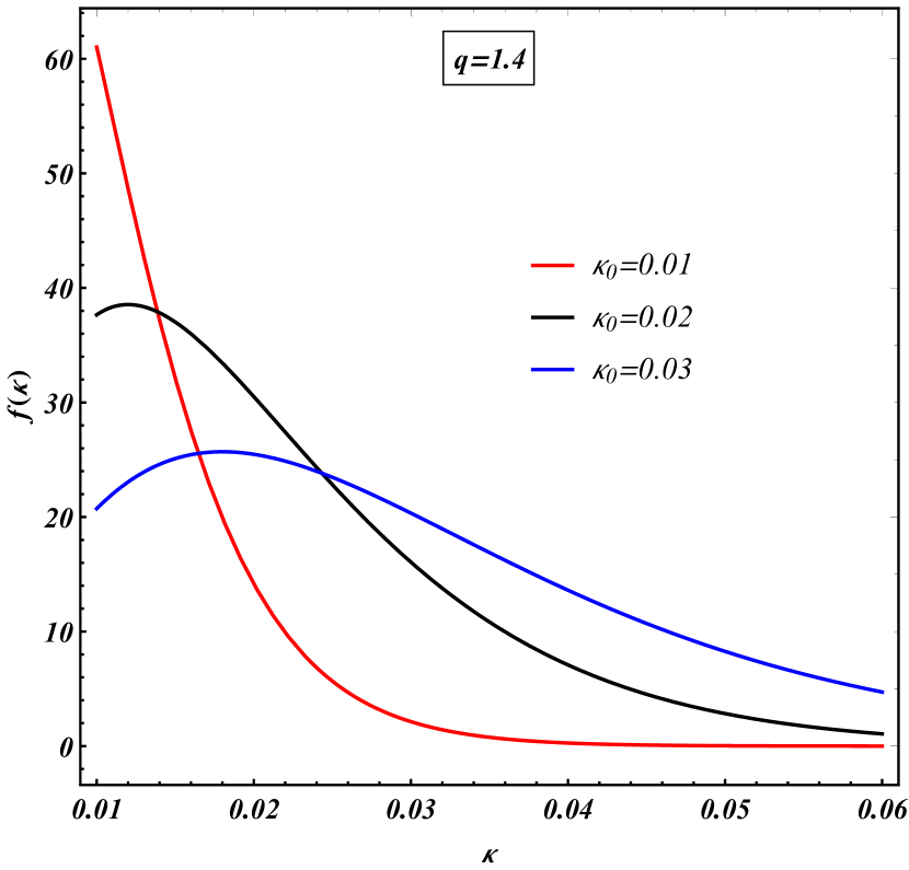
Figure 2: Gamma distributions for a fixed $q$ and different $\kappa_{0}$ values.

II.2 Impulsivity fluctuation in the exponential model and an effective factor

We consider the exponential model of delay discounting given by Eq. (1) and consider that impulsivity $\kappa$ is a fluctuating quantity. Considering that $\kappa$ in Eq. (1) is distributed according to Eq. (2), we can define an ‘effective exponential factor’ (essentially an average) defined by,

$$\epsilon_{\text{eff}} = \frac{\int_{0}^{\infty}d\kappa\exp({-\kappa D})f(\kappa)}{\int_{0}^{\infty}d\kappa f(\kappa)}$$ (4)

$$= \int_{0}^{\infty}d\kappa\exp({-\kappa D})f(\kappa)$$

in which each $\kappa$ in the exponential is now weighted by the normalized distribution $f(\kappa)$.

The factor $\epsilon_{\text{eff}}$ accommodates fluctuating $\kappa$ values (which may range from very small to very large values) already present in a social system. In Eq. (1), we replace the exponential function with $\epsilon_{\text{eff}}$, and propose the effective exponential model given by,

$$V(D)=V(0)\epsilon_{\text{eff}}$$ (5)

Defining an effective exponential factor is the reason why the proposed model is named the ‘effective exponential model’. This approach is used in physical systems wilkprl where temperature is a fluctuating quantity and an effective Boltzmann factor is defined (Boltzmann is exponential). We show that this effective exponential factor is nothing but the Tsallis function. An analytical closed form of $\epsilon_{\text{eff}}$ is obtained as described below.

From Eq. (2) we have,

$$\epsilon_{\text{eff}} = \int_{0}^{\infty}d\kappa\exp({-\kappa D})f(\kappa)$$ (6)

$$= \frac{1}{\Gamma\left(\frac{1}{q-1}\right)}\left\{\frac{1}{(q-1)\kappa_{0}}\right\}\int_{0}^{\infty}d\kappa\exp({-\kappa D})\left\{\frac{\kappa}{(q-1)\kappa_{0}}\right\}^{\frac{1}{q-1}-1}\exp\left(-\frac{\kappa}{(q-1)\kappa_{0}}\right)$$

$$= \frac{1}{\Gamma\left(\frac{1}{q-1}\right)}\left\{\frac{1}{(q-1)\kappa_{0}}\right\}^{\frac{1}{q-1}}\int_{0}^{\infty}d\kappa\exp\left[{-\kappa\left(D+\frac{1}{(q-1)\kappa_{0}}\right)}\right]\kappa^{\frac{1}{q-1}-1}$$

Now, defining $\kappa\left(D+\frac{1}{(q-1)\kappa_{0}}\right)=\kappa^{\prime}$, the above integral can be written as,

$$\epsilon_{\text{eff}} = \frac{1}{\Gamma\left(\frac{1}{q-1}\right)}\left\{\frac{1}{(q-1)\kappa_{0}}\right\}^{\frac{1}{q-1}}\left(D+\frac{1}{(q-1)\kappa_{0}}\right)^{-\frac{1}{q-1}}\int_{0}^{\infty}d\kappa^{\prime}\exp(-\kappa^{\prime})\kappa^{\prime\frac{1}{q-1}-1}.$$ (7)

From Eq. (3), the integral in the above equation is nothing but $\Gamma\left(\frac{1}{q-1}\right)$ and hence,

$$\epsilon_{\text{eff}}=\left(1+(q-1)\kappa_{0}D\right)^{\frac{1}{1-q}}=\exp_{q}(-\kappa_{0}D),$$ (8)

where $\exp_{q}$ is the $q$-exponential function Tsal88 which becomes the conventional exponential function in the limit $q\rightarrow 1$. Hence, a modified form of Eq. (1) is given by,

$$V(D) = V(0)\exp_{q}(-\kappa_{0}D)$$ (9)

$$= \frac{V(0)}{\left(1+(q-1)\kappa_{0}D\right)^{\frac{1}{q-1}}}.~{}~{}~{}~{}~{}~{}\text{(--EEM--)}$$

This is the main result of our paper which describes an ‘effective exponential model (EEM)’ of delay discounting. Takahashi takahashi1 has also proposed a similar Tsallis model. However, there are still some differences among the EEM and the other Tsallis model. We will discuss that in Section III.

II.3 Significance of the parameters $q$ and $\kappa_{0}$

Now, let us investigate what the parameters $\kappa_{0}$ and $q$ signify. As shown next, parameter $\kappa_{0}$ is the mean impulsivity of the system, and $q$ is related to the variance of the impulsivity distribution. From Eq. (2),

$$\langle\kappa\rangle = \int_{0}^{\infty}d\kappa~{}\kappa f(\kappa)$$ (10)

$$= \frac{1}{\Gamma\left(\frac{1}{q-1}\right)}\left\{\frac{1}{(q-1)\kappa_{0}}\right\}^{\frac{1}{q-1}}\int_{0}^{\infty}d\kappa~{}\kappa^{\frac{1}{q-1}}\exp\left(-\frac{\kappa}{(q-1)\kappa_{0}}\right)$$

By defining $k/(q-1)\kappa_{0}=\kappa^{\prime\prime}$ and using Eq. (3) we obtain,

$$\langle\kappa\rangle = \frac{\Gamma\left(\frac{1}{q-1}+1\right)}{\Gamma\left(\frac{1}{q-1}\right)}\times(q-1)\kappa_{0}$$ (11)

$$= \frac{\Gamma\left(\frac{1}{q-1}\right)}{(q-1)\Gamma\left(\frac{1}{q-1}\right)}\times(q-1)\kappa_{0}$$

$$= \kappa_{0}$$

Now, to find out the variance, we need to find out the mean square impulsivity. Again, using Eq. (2) and redefining the integration variable appropriately we obtain,

$$\langle\kappa^{2}\rangle = \int_{0}^{\infty}d\kappa~{}\kappa^{2}f(\kappa)$$ (12)

$$= \frac{1}{\Gamma\left(\frac{1}{q-1}\right)}\left\{\frac{1}{(q-1)\kappa_{0}}\right\}^{\frac{1}{q-1}}\int_{0}^{\infty}d\kappa~{}\kappa^{\frac{1}{q-1}+1}\exp\left(-\frac{\kappa}{(q-1)\kappa_{0}}\right)$$

$$= \frac{\Gamma\left(\frac{1}{q-1}+2\right)}{\Gamma\left(\frac{1}{q-1}\right)}\times(q-1)^{2}\kappa_{0}^{2}$$

$$= q\kappa_{0}^{2}$$

Hence,

$$\frac{\langle\kappa^{2}\rangle-\langle\kappa\rangle^{2}}{\langle\kappa\rangle^{2}}=q-1;~{}~{}\Rightarrow q=1+\frac{\langle\kappa^{2}\rangle-\langle\kappa\rangle^{2}}{\langle\kappa\rangle^{2}}$$ (13)

Eqs. (11) and (13) show that the $\kappa_{0}$ parameter is the mean impulsivity of the sample, and the $q$ parameter is related to the relative variance of impulsivity of the sample. From Eq. (13) it is evident that $q>1$. Hence, the $q\rightarrow 1$ limit signifies a very narrow impulsivity distribution with negligible fluctuation. A similar relation for physical systems can be found in Ref. wilkprl which involves temperature, and Ref. wilkprc which involves particle number.

III Discussion

III.1 Facets of impulsivity

In this article, we consider fluctuations present in a system and we argue that the gamma distribution given by $f(\kappa)$ is the most general distribution of a fluctuating quantity. In that sense, our approach is based on a condition (fluctuation) that is ubiquitous in any system. In a social system, fluctuating impulsivity is a common feature. However, researchers always distinguish between two kinds of impulsivity, trait and state, also called ‘facets’, denoted by $\kappa_{\text{T}}$ and $\kappa_{\text{S}}$ respectively. A trait characteristic is inherent, and a person (or a representative of any other species) is born with it. On the other hand, the state characteristic develops over time and varies. Hence, when one talks about fluctuations, it may seem that she implies the state characteristics only. However, in a study traitstate it has been found that that university soccer players with higher trait anxiety scores may experience increased state anxiety under pressure. Though it discusses a connection between trait and state anxiety, yet it is possible that the trait and state impulsivity are also connected. Hence we consider impulsivity obtained from delay discounting data as a combination of both. That is because a more or less unaltered quantity combined with an alternating quantity gives rise to another alternating quantity.

III.2 Drift and diffusion of impulsivity

It is interesting to note in Figs. 2 and 2 that when we vary $\kappa_{0}$ and $q$ of the distribution, the peak and the width of the distribution changes. This shift in the peak of average impulsivity and width is analogous to the velocity-space drift and diffusion of a collection of particles traversing inside a medium. In this case, the average velocity and the width change because of the interaction with the medium molecules. We can similarly think about the change in the impulsivity distribution in terms of drift and diffusion in the impulsivity space. If we study the time evolution of the impulsivity distribution $f(\kappa)$ of a test sample, it can schematically be written in terms of two terms representing the drift ($\gamma_{\kappa}>0$) and diffusion ($\delta_{\kappa}>0$) in the following way,

$$\dot{f}(\kappa)=-\text{change~{}due~{}to~{}}\gamma_{\kappa}+\text{change~{}due~{}to~{}}\delta_{\kappa},$$ (14)

where the dot on $f(\kappa)$ signifies total time derivative. Time evolution of the impulsivity distribution of a sample may be a consequence of many factors like changing social status, social interaction and so on.

III.3 Comparison of the EEM with another Tsallis-like model

Another Tsallis-like model proposed by Takahashi in Ref. takahashi1 has the following form according to our notations,

$$V(D) = \frac{V(0)}{\exp_{q}\left({\kappa_{0}D}\right)}$$ (15)

$$= \frac{V(0)}{(1+(1-q)\kappa_{0}D)^{\frac{1}{1-q}}}.~{}~{}~{}~{}~{}~{}\text{(--TM--)}$$

Eq. (15) is to be referred to as the Takahashi model (TM) from now on. If $q$ is replaced by $2-q$ in the TM, one obtains the EEM (Eq. 9), and this is the reason why the TM and EEM may be termed as ‘dual to each other’. This duality reminds one of the same correspondence existing between the $q$-exponential function and its inverse eqinv . The EEM relates $q$ to the relative variance of the impulsivity distribution, and it is always positive. However, the $q$ values in the TM model can assume negative values. In spite of the difference in their appearances, it is seen that numerically these two models are equivalent. However, the parameter values in two approaches have a $q\leftrightarrow 2-q$ correspondence because of the dual nature.

There is another subtle difference between the two Tsallis-inspired models which we discuss now. This discussion is based on the fact that we demand $V$ to be a real-valued quantity and not a complex number. From Eq. (9) it is clear that if $1+(q-1)\kappa_{0}D$ is negative, one may get a complex valued quantity because the $q$ parameter (also called the Tsallis parameter or the entropic index) is a real number. For example, for $q=0.1$, $\kappa_{0}=0.2$ and $D=10$, $1+(q-1)\kappa_{0}D=-0.8$ and $\left(1+(q-1)\kappa_{0}D\right)^{1/(1-q)}$ is a complex number. However, since we have $q>1,~{}\kappa_{0}>0$ and $D>0$ in our model (Eq. 9), we do not encounter complex values. The same constraint of positivity of the argument leads to an upper-bound of the $q$ values in the TM,

$$q<1+\frac{1}{\kappa_{0}D}.$$ (16)

III.4 Different limits of the EEM

Now, let us discuss different limits of the effective exponential model. In the limit $q\rightarrow 1$ (vanishing fluctuation), Eq. (9) gives back the exponential model of delay discounting as shown below,

$$\lim_{q\rightarrow 1}V(D) = \lim_{q\rightarrow 1}V(0)\left(1+(q-1)\kappa_{0}D\right)^{-\frac{1}{q-1}}$$ (17)

$$= \lim_{q\rightarrow 1}V(0)\exp\left({-\frac{1}{q-1}\ln\left(1+(q-1)\kappa_{0}D\right)}\right)$$

$$= \lim_{q\rightarrow 1}V(0)\exp\left({-\frac{1}{q-1}\left\{(q-1)\kappa_{0}D-\mathcal{O}(q-1)^{2}+...\right\}}\right)$$

$$= V(0)\exp\left(-\kappa_{0}D\right)$$

When we take the $\kappa_{0}D\rightarrow 0$ limit, Eq. (17) gives back the hyperbolic equation given by,

$$\lim_{\kappa_{0}D\rightarrow 0}V(D)\approx\frac{V(0)}{1+\kappa_{0}D}.$$ (18)

Also, when $q=2$, Eq. (9) gives back the hyperbolic model. Hence the EEM generalizes the existing models of delay discounting which may be obtained by taking appropriate limits of the EEM.

IV Summary, conclusions, and outlook

To summarize, considering impulsivity to be a fluctuating quantity we describe an effective exponential model of delay discounting phenomenon. This model described in the article is found to be dual to the Tsallis model of delay discounting proposed by Takahashi takahashi1 . In that sense, our findings support the existing Tsallis models which efficiently describe different aspects of delay discounting (like the inter-temporal inconsistency) which are important in deciding policies in many sectors like finance, medical etc.

The novelty of our article lies in the approach it takes. We consider a very general characteristic of a system (fluctuation) and propose a modification of the existing exponential model to arrive at another intuitive understanding of the Tsallis model. With the help of this approach we explain the significance of the model parameters. We find that

• the Tsallis parameter $q$ is related to the relative variance (variance divided by average square) of the impulsivity distribution and is greater than 1.

• the impulsivity parameter $\kappa_{0}$ is actually the mean of the impulsivity distribution.

It will be interesting to apply this model for participants from varied age groups and social backgrounds to study how impulsivity changes. It will also be interesting to see how the personality of an individual affects this behavior. From the observations, one may parameterize the evolution the $q$ and $\kappa_{0}$ parameters with age to predict the impulsivity behavior of people from certain age group from a certain socio-cultural background. These findings will be important in deciding policies in relevant areas.

Our study can throw light upon some other interesting aspects of social science in general. We try to elaborate on this in the next few sentences. As mentioned in Section III, we consider impulsivity obtained from delay discounting data to be a combination of trait and state facets. However, how to combine these two facets to get the combination is another interesting question which future researchers may revisit. In many studies it is assumed to be a sum score given by the addition of facets. Since we consider impulsivity to be bi-faceted, the total impulsivity may be given by the sum score of $\kappa_{\text{T}}$ and $\kappa_{\text{S}}$. In that case, one immediately finds that addition is only one of the options among a large number of operators which combine these two numbers. There can also be some other ways to combine the facets. One may propose a gedankenexperiment gedanken in which the trait and state impulsivity of a group of participants are quantified from questionnaires, and the combined impulsivity of the same participants are measured by fitting the data obtained from the delay-discounting experiments using the Tsallis model. From these three sets of numbers, one can try to find out a rule of combining them. This question becomes really important when one needs to score competitors for providing grants, or for providing some aid and in many other situations in which a questionable method of evaluation may be disappointing (for the marginalized section, for example).

We would like to point out that the superstatistics approach may also be taken in describing financial market data using the $q$-gaussian distribution tsfinnewjphys ; tsfinphysrept that is obtained by replacing the exponential function in Eq. (4) by a gaussian. In Refs. tsfinnewjphys ; tsfinphysrept , authors observe that $q$ approaches unity when the time lag increases for the financial return distribution. This can be explained if $q$ can be identified as an internal variable that follows a relaxation-like equation qint ,

$$\frac{dq}{d\delta t}=-\frac{q-q_{\text{eq}}}{\tau},$$ (19)

where $q_{\text{eq}}=1$, $\delta t$ is the time-lag, and $\tau$ is a characteristic time scale. The solution of the above equation yields $q(\delta t)=1+(q_{\text{eq}}-1)e^{-\frac{\delta t}{\tau}}$, and supports the observation.

To conclude, the effective exponential model lends support to the Tsallis model of delay discounting. However, its implications may go way beyond that as discussed in the article. We have provided some insight into the model, and have raised some questions that seemed to be relevant for a deeper understanding. With this input, we hope that future studies will shine more light on this very interesting phenomenon of delay discounting.

References

- (1) A.L. Odum, Delay Discounting: I’m a k, You’re a k, J. Exp. Anal. Behav. 96 (3) (2011) 427-439
- (2) J.E. Mazur, An adjusting procedure for studying delayed reinforcement, in: M.L. Commons, J.E. Mazur, J.A. Nevin, H. Rachlin (Eds.), Quantitative Analysis of Behavior: Vol. 5. The Effect of Delay and of Intervening Events on Reinforcement Value, Hillsdale, NJ: Erlbaum, 1987, pp. 55-73
- (3) H. Rachlin and B. A. Jones, Social Discounting and Delay Discounting, J. Behav. Dec. Making 21 (2008) 29-43
- (4) K.M. Lempert, and D.A. Pizzagalli, Delay discounting and future-directed thinking in anhedonic individuals, J. Behav. Ther. & Exp. Psychiat. 41 (2010) 258-264
- (5) B.J. West and P. Grigolini, A psychophysical model of decision making,Physica A 389 (2010) 3580-3587
- (6) D.O. Cajueiro, A note on the relevance of the q-exponential function in the context of intertemporal choices, Physica A 364 (2006) 385-388
- (7) A. Tversky and D. Kahneman, Rational Choice and the Framing of Decisions, The Journal of Business Vol. 59, No. 4, Part 2: The Behavioral Foundations of Economic Theory (Oct., 1986), pp. S251-S278 (28 pages)
- (8) H. Rachlin, Notes on discounting. Journal of The Experimental Analysis of Behavior, 85 (2006) 425-435.
- (9) T. Takahashi, A comparison of intertemporal choices for oneself versus someone else based on Tsallis’ statistics, Physica A 385 (2007) 637-644
- (10) V.I. Yukalov and D. Sornette, Physics of uncertainty in Quantum Decision Making, The European Physical Journal B, 71 No. 4 (2009) pp. 533-548.
- (11) T. Takahashi, A social discounting model based on Tsallis’ statistics, Physica A 389 (2010) 3600-3603
- (12) T. Takahashi, H. Nishinaka, T. Makino, R. Han and H. Fukui, An Experimental Comparison of Quantum Decision Theoretical Models of Intertemporal Choice for Gain and Loss, Journal of Quantum Information Science 2 (2012) 119-122
- (13) K. Ishii and C. Eisen, Cultural Similarities and Differences in Social Discounting: The Mediating Role of Harmony-Seeking, Frontiers in Psychology 9 (2018) 1426
- (14) S.E. Stegall, T. Collette, T. Kinjo, T. Takahashi and P. Romanowich, Quantitative Cross-Cultural Similarities and Differences in Social Discounting for Gains and Losses, Frontiers in Public Health 7 (2019) 297
- (15) I.M.P. Oller, S.C. Rambaud and M.d.C.V. Martinez, Discount models in intertemporal choice: an empirical analysis, European Journal of Management and Business Economics, 30 No. 1 (2021) pp. 72-91
- (16) C.Beck and E.G.D.Cohen, Superstatistics, Physica A: Statistical Mechanics and its Applications, Volume 322 (2003) 267-275
- (17) G. Wilk, and Z. Włodarczyk, Interpretation of the nonextensivity parameter q in some applications of tsallis statistics and lèvy distributions, Phys. Rev. Lett. 84 (2000) 2770-2773
- (18) R.V. Hogg, J.W. McKean, A.T. Craig, Introduction to Mathematical Statistics, Pearson Education, Boston (2019)
- (19) C. Tsallis, Possible generalization of Boltzmann-Gibbs statistics, J. Stat. Phys. 52 (1988) 479-487
- (20) G. Wilk, and Z. Włodarczyk, Multiplicity fluctuations due to the temperature fluctuations in high-energy nuclear collisions, Phys. Rev. C 79 (2009) 054903
- (21) M. Horikawa, A. Yagi, The Relationships among Trait Anxiety, State Anxiety and the Goal Performance of Penalty Shoot-Out by University Soccer Players, PLOS ONE, Volume 7 Issue 4 (2012) e35727
- (22) as can be seen from Eq. (8).
- (23) https://www.britannica.com/science/Gedankenexperiment
- (24) Stanisław Drożdż, Jarosław Kwapień, Paweł Oświȩcimka and Rafał Rak, The foreign exchange market: return distributions, multifractality, anomalous multifractality and the Epps effect, New J. Phys. 12 (2010) 105003 (23pp).
- (25) Jarosław Kwapień and Stanisław Drożdż, Physical approach to complex systems, Phys. Rep. 515 (2012) 115-226.
- (26) V. N. Pokrovski, ISRN Thermodynamics, ID 906136 (2013).