Superconductivity in the vicinity of an isospin-polarized state in a cubic Dirac band

Abstract

We present a theory of superconducting pairing originating from soft critical fluctuations near isospin-polarized states in rhombohedral trilayer graphene. Using a symmetry-based approach, we determine possible isospin order types and derive the effective electron-electron interactions mediated by isospin fluctuations. Superconductivity arising due to these interactions has symmetry and order parameter structure that depend in a unique way on the “mother” isospin order. This model naturally leads to a superconducting phase adjacent to an isospin-ordering phase transition, which mimics the behavior observed in experiments. The symmetry of the paired state predicted for the isospin order type inferred in experiments matches the observations. These findings support a scenario of superconductivity originating from electron-electron interactions.

The nature of superconductivity (SC) observed in moiré grapheneCao1 has been a topic of intense interest in recent years.Balents_review_TBG Initially, the resemblance between phases diagram in moiré graphene and cuprates suggested a non-phonon mechanism of pairingCao1 , a scenario supported by theoretical investigation of various types of interaction-driven SCDodaro ; Xu ; Guinea ; CCLiu ; Guo ; You_SC ; Girish . Meanwhile, it was noted that the phonon-mediated coupling may be strong enough to explain the observed SCWu1 ; Wu2 ; Peltonen ; Lian . Subsequent experiments painted a more complex pictureCao2 ; Dmitri1 ; Saito2020 ; Stepanov ; XLiu , initiating an ongoing debate.

The recently discovered superconductivity in rhombohedral trilayer graphene (RTG)HZhou2 offers clues that go a long way towards solving this puzzle. Though the band structures of RTG and moiré graphene are completely distinct, SC in RTG appears at ultralow carrier densities and relatively high temperatures.HZhou2 This is so because the density of states at low doping where SC occurs is dominated by an extremely flat top of the hole band, reaching values as high as those in moiré bands.Koshino ; FZhang Interestingly, the key aspects of the phase diagrams of RTG and moiré graphene resemble each other. In moiré graphene, the SC domes are found amid a cascade of ordered phases.Cao1 Likewise, the phase diagram of RTG is packed with various ordered phasesHZhou1 with the SC phases located along the lines where symmetry-breaking phase transitions into isospin-polarized states occur. E.g. one SC phase (called SC1 in HZhou1 ) appears at the transition from the disordered state with four-fold Fermi sea degeneracy to a valley-polarized state with a two-fold degenerate Fermi sea. Another SC phase (SC2) is found at the transition from a two-fold degenerate Fermi sea to a non-degenerate one.

The RTG has several appealing aspects as a platform to explore the interplay between strongly correlated phases and superconductivity. Moiré graphene hosts a variety of twist-related defects, such as twist-angle disorderWilson ; Uri , heterostrainMesple ; Huder ; Cosma ; ZBi and bucklingSZhou ; Uchida ; Butz , that can strongly affect the bandstructure in the moiré flatbands. In comparison, RTG is a clean system free of this type of defects. In addition, the band dispersion and electron wavefunctions in moiré materials are fairly cumbersome, whereas the RTG enjoys a much simpler band structureKoshino ; FZhang , allowing for analytical modeling.

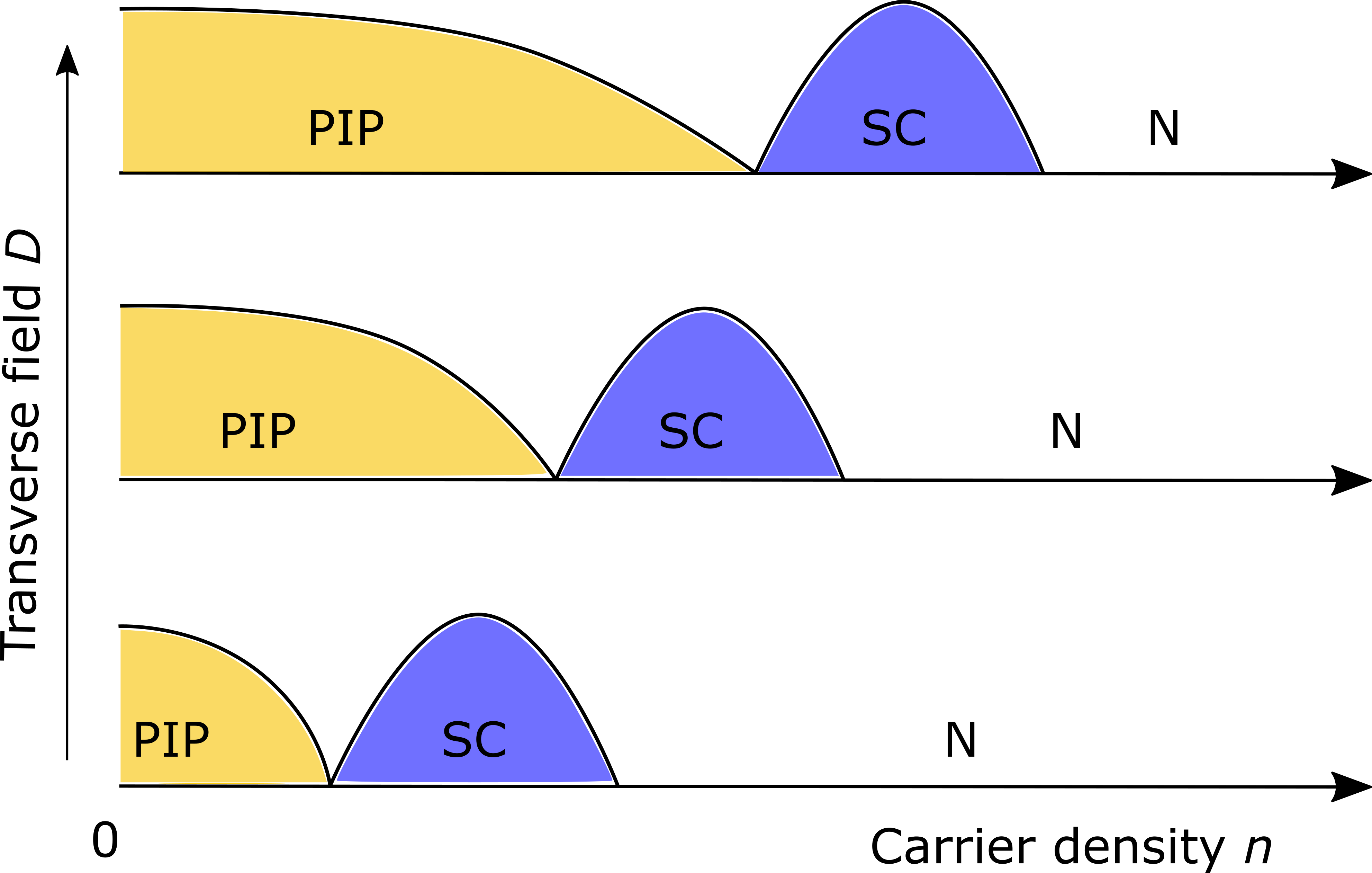
Figure 1: Phase diagram predicted from the model of superconductivity in RTG mediated by critical fluctuations in the partially isospin polarized phase (PIP). The pairing interaction is strongest at the phase boundary between the PIP phase and the unpolarized phase (N), leading to superconductivity (SC) near the PIP phase onset.

With this motivation in mind, here we aim at developing a framework capable of predicting the correct superconducting orders in RTG. Accounting for the fact that all SC phases in RTG are located at the vicinity of phase boundaries of isospin-ordered phases, we will treat these phases as “mother states” for the corresponding SC orders, and explore the scenario that the critical fluctuations of the order parameter act as a pairing glueChubukov_review ; Scalapino . Unlike the more conventional scenariosKopnin2011 ; Chou our framework naturally explains the intimate relation between SC and ordered states observed in experiment. The first step of our analysis is to consider possible orders in the mother state. Taking the SC1 state as an illustration, and using a symmetry-based approach, we identify a symmetry-breaking phase with the characteristics matching those of the valley-polarized spin-unpolarized phase (labeled PIP in Ref.HZhou2, ) near which the SC1 phase is observed. The electron-electron interactions that mediate pairing arise from critical fluctuations, leading to superconductivity near the onset of the order in the partially polarized phase, as illustrated in Fig.1. This framework unambiguously predicts a spin-singlet superconductivity, which is compatible with the Pauli-limited SC observed in experimentHZhou2 . This approach allows a straightforward generalization to describe the interplay between other observed SC phases and their “mother states.”

Although the general idea of fluctuation-mediated pairing is similar to the mechanism studied in iron superconductors,Hosono_review ; Kuroki ; Mazin there are some crucial differences. Namely, in iron pnictides, the pairing arises mainly from the pairing-hopping process in which a Cooper pair on one Fermi pocket absorb the momentum of a soft mode and hops to the other Fermi pocketKuroki ; Mazin . In comparison, in our theory for RTG, the Cooper pairs consist of two electrons from opposite valleys $K$ and $K^{\prime}$. In the process that leads to pairing, two paired electrons exchange valleys as $K,K^{\prime}\to K^{\prime},K$, a process mediated by a soft mode that carries finite momentum $\pm 2K$.

We start by writing down the Hamiltonian of electrons in RTG. Restricted by the space-group symmetry, the electron Hamiltonian takes the following form:Supplement

$$H=\sum_{{\boldsymbol{p}}}\Psi_{{\boldsymbol{p}}}^{\dagger}M({\boldsymbol{p}})\Psi_{{\boldsymbol{p}}},$$

$$M({\boldsymbol{p}})=h_{0}({\boldsymbol{p}})1\sigma_{1}+h^{\prime}_{0}({\boldsymbol{p}})1_{4}+h_{3}({\boldsymbol{p}})1\sigma_{3}+$$

$$+h_{1}({\boldsymbol{p}})\left(\alpha\tau_{3}\sigma_{1}+\alpha^{\prime}\tau_{3}1+\alpha^{\prime\prime}\tau_{3}\sigma_{3}\right)+h_{2}({\boldsymbol{p}})1\sigma_{2}$$ (1)

where $\Psi_{{\boldsymbol{p}}}=\left(\psi_{{\boldsymbol{p}},KA},\psi_{{\boldsymbol{p}},KB},\psi_{{\boldsymbol{p}},K^{\prime}A},\psi_{{\boldsymbol{p}},K^{\prime}B}\right)^{T}$, $\tau_{i}$’s are Pauli matrices in $K$ and $K^{\prime}$ valley basis, $\sigma_{i}$’s are Pauli matrices in sublattice (layer) basis [$i=0,1,2,3$, $\sigma_{0}=\tau_{0}=1_{2}$]. The quantities $h_{n}$’s are defined asKoshino ; FZhang

$$h_{0}({\boldsymbol{p}})=\Delta+\frac{p^{2}}{2m},\quad h^{\prime}_{0}({\boldsymbol{p}})=\Delta^{\prime}+\frac{p^{2}}{2m^{\prime}},$$

$$h_{1}({\boldsymbol{p}})=p_{1}^{3}-3p_{1}p_{2}^{2},\quad h_{2}({\boldsymbol{p}})=\beta\left(3p_{1}^{2}p_{2}-p_{2}^{3}\right),$$

$$h_{3}({\boldsymbol{p}})=D+\frac{p^{2}}{2m_{3}}.$$ (2)

Below, rather than using the realistic valuesKoshino ; FZhang , we set $h_{0}=h_{0}^{\prime}=\alpha^{\prime}=\alpha^{\prime\prime}=0$ and $m_{3}=\infty$. As we will see, this choice of parameters represents a simplest case that allows one to reproduce a qualitatively correct phase diagram while keeping the analysis simple. For this choice of parameters, the Hamiltonian becomes

$$H=\sum_{{\boldsymbol{p}}}\Psi_{{\boldsymbol{p}}}^{\dagger}\left[h_{1}({\boldsymbol{p}})\tau_{3}\sigma_{1}+h_{2}({\boldsymbol{p}})1_{2}\sigma_{2}+D1_{2}\sigma_{3}\right]\Psi_{{\boldsymbol{p}}}$$ (3)

The resulting band structure is shown in Fig.2. Discarding $h^{\prime}_{0}$ and $h^{\prime}_{1}$ makes our model Eq.(3) particle-hole symmetric $E_{p}({\boldsymbol{p}})=-E_{h}({\boldsymbol{p}})$. For later convenience, we define the absolute value of the energy in the two bands:

$$E({\boldsymbol{p}})=E_{p}({\boldsymbol{p}})=-E_{h}({\boldsymbol{p}})=\sqrt{h_{0}({\boldsymbol{p}})^{2}+h_{2}({\boldsymbol{p}})^{2}+D^{2}}.$$ (4)

We note that, while the realistic system is not particle-hole symmetric, the measured RTG phase diagrams on the electron-doped and hole-doped regimes are qualitatively similar — they both host cascades of ordered statesHZhou1 and superconducting phasesHZhou2 . We therefore proceed with the model in Eq.3.

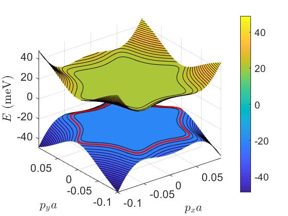
Figure 2: Band dispersion for one valley given by the Hamiltonian in Eq.(3), obtained for realistic parameter values: $D=20$meV, $\alpha/a^{3}=10$eV, $\beta/a^{3}=20$eV, where $a$ denotes the graphene monolayer carbon-carbon spacing $a=1.4\AA$. The red contour marks a Fermi surface at a carrier density comparable to that in experimentsHZhou1 ; HZhou2 .

Next, we introduce electron-electron interactions. For the maximal simplicity, we will only consider a local density-density interaction:

$$H_{\rm int}=V_{0}\sum_{{\boldsymbol{p}}{\boldsymbol{p}}^{\prime}{\boldsymbol{q}}}:\Psi_{{\boldsymbol{p}}+{\boldsymbol{q}}}^{\dagger}1_{4}\Psi_{{\boldsymbol{p}}}\Psi_{{\boldsymbol{p}}^{\prime}-{\boldsymbol{q}}}^{\dagger}1_{4}\Psi_{{\boldsymbol{p}}^{\prime}}:,$$ (5)

where colons indicate normal ordering and the interaction constant $V_{0}$ is positive, corresponding to a repulsion.

For weakly dispersing $E({\boldsymbol{p}})$ this interaction results in a Stoner instability towards a valley-polarized phase. As an illustration, we consider the limit of a large transverse field $D$ for which the band can be viewed as consisting of two parts: a flat bottom and a steep higher-energy part — a toy model inspired by the bandstructure in Fig.2. We will denote the carrier density at which the transition between the two parts occurs as $n_{0}$, which is a function of $D$. In this toy model, we consider only two species: pseudospin up and down ($\uparrow$, $\downarrow$) and assume that electrons only interact with electrons of the same species through an exchange interaction $V<0$. Let $\nu_{0}$ denote the density of states for each species at Fermi surface, and $\nu_{1}$ and $\nu_{2}$ be the density of states for each species in the flat and steep parts respectively ($N_{1}\gg N_{2}$). Consider the energy change due to an infinitesimal polarization $n_{\uparrow}=n+\delta n,n_{\downarrow}=n-\delta n$:

$$\delta E=2\delta n^{2}/\nu_{0}+2V\delta n^{2}$$ (6)

Instability occurs when $\delta E<0$, a condition that gives the Stoner criterion $|V|\nu_{0}>1$. Thus, so long as $\nu_{1}<|V|^{-1}<\nu_{2}$, the instability will occur when $n<n_{0}(D)$. Given that $n_{0}$ monotonically increases with $D$, the Stoner transition threshold dependence on $D$ is monotonic and approximately linear, as illustrated in Fig.1.

However, since in RTG there are two valley species and two layer degrees of freedom, the ordering can take a more complicated form, e.g. a valley-only or layer-only polarization. Determining the order in the mother state is crucial, since it is the form of the mother state that determines the pairing interaction.

The key question is therefore to identify the orbital channel that has the strongest Stoner instability. To address this question, we consider the Stoner criterion for an arbitrary orbital order $\langle\Psi_{{\boldsymbol{p}}}^{\dagger}O\Psi_{{\boldsymbol{p}}}\rangle$:

$$-V_{0}\int\frac{d\omega}{2\pi}\int\frac{d^{2}p}{\left(2\pi\right)^{2}}G(i\omega,p)OG(i\omega,p)=O$$ (7)

where $G(i\omega,p)$ is the electron’s Green’s function, and $O$ is a general complex-valued $4\times 4$ matrix.

The multitude of possible ordered states calls for a symmetry-based approach. The system is invariant under the space group P3m1 which is comprised of the point group $C_{3v}$ and translations. The three-fold rotation operator $C_{3}$ leaves the Dirac spinors $\Psi$ invariant, whereas the mirror operator $\sigma_{d}$ swaps $K$ and $K^{\prime}$ valleys. Translation generates a valley-dependent phase factor when hitting Dirac spinors. From this we can see how Dirac particle-hole bilinears transform under the space group. Namely, the valley-diagonal part of the $O$ matrix contains components that transform under $A_{1}$ and $A_{2}$ representations of $C_{3v}$, and are invariant under lattice translations. The valley-off-diagonal part of $O$ matrix contains components that transform under the symmetry group of $K$ point since the total momentum of an intervalley particle-hole pair is $2K$ (or, equivalently $-K$). This yields all possible $O_{ij}$ that can be decomposed into three 1D representations $A_{1,\Gamma}$, $A_{2,\Gamma}$ and $A_{\pm K}$ of the space group. Further classifying them by whether they are even or odd under time reversal (represented by superscripts $+,-$), we findSupplement a list of irreducible representations and PIP states with different symmetries given in Table 1 (a similar analysis can be found in Ref.Vafek, ). Guided by experiment, here we focus on the spin-unpolarized PIP states.

irrep	Isospin-polarized state orders $O$
$A_{1,\Gamma}^{+}$	$1_{4},1\sigma_{1},1\sigma_{3}$
$A_{1,\Gamma}^{-}$	$1\sigma_{2}$
$A_{2,\Gamma}^{+}$	$\tau_{3}\sigma_{2}$
$A_{2,\Gamma}^{-}$	$\tau_{3}1,\tau_{3}\sigma_{1},\tau_{3}\sigma_{3}$
$A_{\pm K}^{+}$	$\tau_{1}\sigma_{n},\tau_{2}\sigma_{n}$, ($n=0,1,3$)
$A_{\pm K}^{-}$	$\tau_{1}\sigma_{2},\tau_{2}\sigma_{2}$

Table 1: Symmetry classification of different partially isospin-polarized and spin-unpolarized (PIP) states (see text).

To understand which of these orders win over other orders we combine the symmetry analysis with the Stoner criterion, Eq.7. On general grounds,Supplement the problem of finding the channels with the strongest Stoner instability is equivalent to maximizing the quadratic function

$$F[O]=-\int\frac{d\omega}{2\pi}\frac{d^{2}p}{\left(2\pi\right)^{2}}\frac{1}{4}{\rm\,Tr\,}\left[O^{\dagger}G(i\omega,p)OG(i\omega,p)\right]$$ (8)

subject to the normalization constraint $\frac{1}{4}{\rm\,Tr\,}O^{\dagger}O=1$. Expanding $O$ over the basis of Pauli matrices: $O=d_{ij}\tau_{i}\sigma_{j}$, where $d_{ij}$’s are complex valued, we write $F$ into a quadratic form of $d_{ij}$. Maximizing this quadratic form is straightforward since it is diagonal in terms of $d_{ij}$Supplement . In this way, we identify the following two channels which have the strongest instability:

$$O=\tau_{1}\sigma_{1},\tau_{2}\sigma_{1}.$$ (9)

Since the two candidate order parameters transform under 1D representations of the space group, their degeneracy is accidental, i.e. not protected by symmetry. We therefore conclude that the order parameter will be either $\tau_{1}\sigma_{1}$ or $\tau_{2}\sigma_{1}$ and not a superposition of the two — if one of them is condensed, the other will be gapped out. We therefore only need to consider these two possibilities.

Interestingly, both candidate Stoner channels correspond to some valley-coherent order, which matches the observation of the partially isospin polarized (PIP) ordered phase in experiment.HZhou2 However, which one is ultimately chosen can not be determined unless we introduce a more complicated model, which is beyond the scope of this paper. Here we proceed by taking one of them, $O=\tau_{1}\sigma_{1}$, as the order parameter of the mother state. In the Supplement, we show that this choice does not impact our conclusion about superconducting order.

With this, we can move on to consider the effective e-e interaction generated due to the proximity to this ordered mother state. Similar scenarios have been studied in other systems.Scalapino ; Bickers ; Moriya1 ; Moriya2 ; Oganesyan ; Roussev ; Kim ; Chubukov ; Chubukov_review ; DellAnna ; Lederer1 ; Lederer2 Here we employ a scalar-electron coupling model, which is similar to the spin-fermion model studied in literature.Chubukov ; Chubukov_review ; Lederer1 ; Lederer2 Namely, we introduce a scalar $\phi$ to represent the order of mother state. The field $\phi$ is softened and fluctuates strongly near the Stoner instability. The Hamiltonian describing the soft mode $\phi$ can be phenomenologically written as

$$H_{s}=\frac{1}{2}|\partial_{t}\phi|^{2}+\frac{K}{2}|\partial_{x}\phi|^{2}+\frac{J}{2}|\phi|^{2}+\frac{U}{2}|\phi|^{4},$$ (10)

where $U$ is always positive, $J>0$ outside $\tau_{1}\sigma_{1}$ phase, $J<0$ inside $\tau_{1}\sigma_{1}$ phase. This Hamiltonian describes a soup of soft-mode fluctuations near the Stoner transition. These coupling between these fluctuations and electrons moving on top of them can be written phenomenologically as

$$H_{e-s}=\gamma\sum_{{\boldsymbol{p}}{\boldsymbol{q}}}\phi_{{\boldsymbol{q}}}\psi_{{\boldsymbol{p}}+{\boldsymbol{q}}}^{\dagger}\tau_{1}\sigma_{1}\psi_{{\boldsymbol{p}}}+{\rm h.c.},$$ (11)

This expression, which respects the space group symmetry, yields a soft-mode-mediated e-e interaction represented by the following term in system action:Supplement

$$A_{ee}(\Psi,\overline{\Psi})=\frac{1}{2}\sum_{\omega,{\boldsymbol{p}}}\tilde{V}_{i\omega,p}\rho^{11}_{i\omega,{\boldsymbol{p}}}\rho^{11}_{-i\omega,-{\boldsymbol{p}}},$$ (12)

where $\rho^{11}_{i\omega,{\boldsymbol{p}}}=\sum_{i\nu,{\boldsymbol{k}}}\overline{\Psi}_{i\nu+i\omega,{\boldsymbol{k}}+{\boldsymbol{p}}}\tau_{1}\sigma_{1}\Psi_{i\nu,{\boldsymbol{k}}}$, and $\Psi_{i\nu,{\boldsymbol{k}}}$, $\overline{\Psi}_{i\nu,{\boldsymbol{k}}}$ are fermionic fields describing Dirac electrons, and

$$\tilde{V}_{i\omega,p}=\begin{cases}\frac{\gamma^{2}}{-\omega^{2}-\omega_{p\parallel}^{2}}+\frac{\gamma^{2}}{-\omega^{2}-\omega_{p\perp}^{2}},\quad\text{inside $\tau_{1}\sigma_{1}$ phase},\\ \frac{2\gamma^{2}}{-\omega^{2}-\Omega_{p}^{2}},\quad\text{outside $\tau_{1}\sigma_{1}$ phase},\end{cases}$$

$\Omega_{p}=\sqrt{Kp^{2}+J}$, $\omega_{p\perp}=\sqrt{K}p$, $\omega_{p\parallel}=\sqrt{Kp^{2}-2J}$. Importantly, the interaction $\tilde{V}(i\omega,p)$ is of a negative sign (an attraction), and is maximized near the phase boundary. In $\tau_{1}\sigma_{1}$ phase, the first term arises from amplitude fluctuation of $\phi$, while the second terms arises from the phase fluctuation of $\phi$. Outside $\tau_{1}\sigma_{1}$ phase, fluctuations along two directions in complex plane contribute equally.

Below, for illustration, we will ignore the momentum and frequency dependence of $\tilde{V}(i\omega,p)$, and work with the following simplified effective e-e interaction:

$$H_{ee}=\sum_{{\boldsymbol{p}},{\boldsymbol{k}},{\boldsymbol{k}}^{\prime}}\tilde{V}:\Psi^{\dagger}_{{\boldsymbol{k}}^{\prime}+{\boldsymbol{p}}}\tau_{1}\sigma_{1}\Psi_{{\boldsymbol{k}}^{\prime}}\Psi^{\dagger}_{{\boldsymbol{k}}-{\boldsymbol{p}}}\tau_{1}\sigma_{1}\Psi_{{\boldsymbol{k}}}:$$ (13)

where $\tilde{V}$ is a negative constant estimated above.

It is important to note that, while the isospin-ordered state acts as a mother state for the SC order through providing pairing glue, the spatial symmetries of these states are in general not directly related. This is so because SC arises outside the isospin-ordered phase — before the symmetry-breaking ordering occurs. Namely, the soft-mode-mediated pairing interaction respects the full symmetry of the space group. Starting from such a maximally symmetric Hamiltonian, the first symmetry that breaks in SC phase is not necessarily the same as the symmetry of the soft mode that has not condensed yet.

With this in mind, we proceed to develop a symmetry-based analysis of SC order. Using Eq.(13), the linearized pairing gap equation in an arbitrary pairing channel $\langle\Psi^{T}\tilde{O}\Psi\rangle$ can be written as

$$-\int\frac{d\omega}{2\pi}\frac{d^{2}p}{\left(2\pi\right)^{2}}\tilde{V}O^{T}G^{T}(-i\omega,-p)\tilde{O}G(i\omega,p)O=\tilde{O},$$ (14)

where $O=\tau_{1}\sigma_{1}$ is the isospin-polarized state found above and $\tilde{O}$ is an arbitrary complex-valued $4\times 4$ matrix.

Possible SC orders, classified according their symmetries, are listed in Table2. Our goal is to find the one which is most unstable to pairing. Due to the resemblance between Eq.(14) and Eq.(7), we will proceed in a similar fashion. First, similar to our analysis of Eq.(7), we can convert the problem of the most unstable pairing channel to a problem of maximizing a quadratic function

$$\tilde{F}[\tilde{O}]=-\int\frac{d\omega d^{2}p}{\left(2\pi\right)^{3}}\frac{1}{4}{\rm\,Tr\,}\left[\tilde{O}^{\dagger}O^{T}G^{T}(-i\omega,-p)\tilde{O}G(i\omega,p)O\right]$$ (15)

subject to the normalization constraint $\frac{1}{4}{\rm\,Tr\,}\tilde{O}^{\dagger}\tilde{O}=1$.

Next, we expand $\tilde{O}$ over a Pauli matrix basis $\tilde{O}=\tilde{d}_{ij}\tau_{i}\sigma_{j}$ ($i,j=0,1,2,3$) where $\tilde{d}_{ij}$’s are complex numbers. Thus, $\tilde{F}$ can be written into a quadratic form of $\tilde{d}_{ij}$. The only off-diagonal terms in this quadratic form are $d_{i3}^{*}d_{i0}$ and $d_{i0}^{*}d_{i3}$. This fact restricts the candidate channels to take one of the following forms

$$\tilde{O}=\tau_{n}\sigma_{1},\tau_{n}\sigma_{2},\tau_{n}(\xi 1+\eta\sigma_{3})$$ (16)

where $\xi$ and $\eta$ are complex numbers. Evaluating $\tilde{F}$ in the first two cases, and maximizing $\tilde{F}$ by varying $\xi,\eta$ in the third case, we ultimately find that the most unstable pairing channel is

$$\tilde{O}=\tau_{1}(\xi_{*}1+\eta_{*}\sigma_{3}).$$ (17)

The explicit form of $\xi_{*}$ and $\eta_{*}$, which is of little relevance for our discussion, is given in the SupplementSupplement .

The SC order in Eq.(17) corresponds to the irreducible representation $A^{+}_{1,\Gamma}$ which preserves all spatial symmetries. The anticommutation constraint for electrons restricts this pairing channel to be a spin-singlet, which is in agreement with the Pauli-limited SC observed in experiment in the SC1 phase.

irrep	superconducting orders $\tilde{O}$
	spin singlet	spin triplet	spatial symmetry
$A_{1,\Gamma}^{+}$	$\tau_{1}1,\tau_{1}\sigma_{1},\tau_{1}\sigma_{3}$	–	no symmetries broken
$A_{1,\Gamma}^{-}$	–	$\tau_{1}\sigma_{2}$
$A_{2,\Gamma}^{+}$	–	$\tau_{2}1,\tau_{2}\sigma_{1},\tau_{2}\sigma_{3}$	reflection symmetry broken
$A_{2,\Gamma}^{-}$	$\tau_{2}\sigma_{2}$	–
$A_{\pm K}^{+}$	$1_{4},1\sigma_{1},1\sigma_{3}$	$\tau_{3}\sigma_{2}$	pair density wave
$A_{\pm K}^{-}$	$\tau_{3}1,\tau_{3}\sigma_{1},\tau_{3}\sigma_{3}$	$1\sigma_{2}$

Table 2: Superconducting order parameters classified by symmetries.Sigrist The SC order found in Eq.(17) belongs to the $A^{+}_{1,\Gamma}$ representation, which preserves the full space group symmetry. Its spin structure is unambiguously a singlet, in line with experimental observations.

Before closing, we comment on the unique testable signatures of SC induced by critical fluctuations. The pairing interaction is due to a collective mode with momenta $\sim 2K$ that softens near the isospin-polarization instability. Electrons in different valleys interact by exchanging such soft excitations, generating pair hopping of the form $(K,K^{\prime})\to(K^{\prime},K)$, $(K^{\prime},K)\to(K,K^{\prime})$. In the process the momentum of each electron changes by $\pm 2K$, a value large on the scale of $k_{F}$ and the typical Thomas-Fermi screening parameter. This suggests that introducing screening by a proximal gateStepanov ; XLiu can serve as a direct test of the pairing mechanism. Indeed, only the relatively long-wavelength harmonics of Coulomb interaction are screened by a gate whereas the harmonics responsible for the $\sim 2K$ momentum transfer remain unscreened. Since the long-wavelength harmonics, which are screened out, are responsible for a pair breaking effect in the Cooper channel, we expect SC to be enhanced upon the introduction of screening. An observation of such SC enhancement would facilitate identifying the unconventional pairing mechanism.

In summary, superconductivity driven by critical soft modes of isospin-polarized states appears to be a viable framework to understand the interplay between different correlated states in RTG, in particular superconductivity observed near the phase boundaries of the isospin-polarized states.HZhou1 ; HZhou2 Our symmetry-based approach singles out an isospin-polarized state with a $K$-$K^{\prime}$ valley coherence which plays a role of a mother state for SC. Accounting for pairing mediated by critical fluctuations in this state predicts the correct order in the SC1 phase, in line with experimental observations.HZhou1 ; HZhou2 This framework is generic and will be straightforward to generalize to other isospin-polarized orders observed in RTG, in particular, the state “SC2” that occurs at an interface between so-far-poorly-understood phases with partially and fully polarized isospin. A SC phase originating from an isospin-polarized phase with broken time reversal symmetry is expected to be a spin-triplet (and, likely, have a p-wave orbital structure). This is consistent with the observation of SC2 phase being resilient under magnetic fields well in excess of the Pauli threshold fields. Generalizing this approach to describe pairing in other phases is an interesting direction for future work. Once confirmed, it will lend strong support to superconductivity arising exclusively from repulsive interactions.

We thank A. V. Chubukov, V. Cvetkovic, O. Vafek and A. F. Young for useful discussions. After the completion of this work two papers appeared on the arXiv proposing other repulsion-based SC scenarios.Ghazaryan ; Chatterjee

I Supplementary Information

I.1 Symmetry analysis of rhombohedral trilayer graphene (RTG) with a transverse field

In this section, we will derive the form of a single-particle Hamiltonian of RTG in a transverse field and discuss its symmetry properties. The symmetry of RTG in the absence of transverse field is $P\overline{3}m1$.Vafek Turning on a transverse field breaks the $C_{2}$ rotation symmetry that swaps the $A$ and $B$ sites in the top and bottom layers. At the same time the mirror symmetries $\sigma_{d}$ with the mirror planes along the directions of AB bonds remain unbroken. As a result, the space group is lowered to $P3m1$. Then the little group for $\Gamma$ point becomes $C_{3v}$; the little group for $\pm K$ points becomes $C_{3}$. The character tables of $C_{3v}$ and $C_{3}$ are listed below

$C_{3v}$	1	$2C_{3}$	$3\sigma_{d}$
$A_{1}$	1	1	1
$A_{2}$	1	1	-1
$E$	2	-1	0

$C_{3}$	1	$C_{3}$	$C_{3}^{2}$
$A$	1	1	1
$E_{1}$	1	$\omega$	$\omega^{*}$
$E_{2}$	1	$\omega^{*}$	$\omega$

Table 3: Character tables for point groups $C_{3v}$ and $C_{3}$, where $\omega=-\frac{1}{2}+\frac{\sqrt{3}}{2}i$, $\omega^{*}=-\frac{1}{2}-\frac{\sqrt{3}}{2}i$.

irrep	Dirac bilinears	function of $p$
$A_{1,\Gamma}^{+}$	$1_{4},1\sigma_{1},1\sigma_{3}$	$1,p^{2}$
$A_{1,\Gamma}^{-}$	$1\sigma_{2}$	$|p|^{3}\sin{3\phi_{p}}=3p_{1}^{2}p_{2}-p_{2}^{3}$
$A_{2,\Gamma}^{+}$	$\tau_{3}\sigma_{2}$	–
$A_{2,\Gamma}^{-}$	$\tau_{3}1,\tau_{3}\sigma_{1},\tau_{3}\sigma_{3}$	$|p|^{3}\cos{3\phi_{p}}=p_{1}^{3}-3p_{1}p_{2}^{2}$
$A_{\pm K}^{+}$	$\tau_{1}\sigma_{n},\tau_{2}\sigma_{n}$, ($n=0,1,3$)	–
$A_{\pm K}^{-}$	$\tau_{1}\sigma_{2},\tau_{2}\sigma_{2}$	–

Table 4: The Dirac bilinears and functions of momentum $p$ classified according to the irreducible representations of the space group $P3m1$.

Below, we determine the form of the single-particle Hamiltonian allowed by symmetry. The Hamiltonian is a bilinear quantity in Dirac spinors $\Psi_{{\boldsymbol{p}}}=(\psi_{{\boldsymbol{p}}AK},\psi_{{\boldsymbol{p}}BK},\psi_{{\boldsymbol{p}}AK^{\prime}},\psi_{{\boldsymbol{p}}BK^{\prime}})^{T}$, defined so that the momentum ${\boldsymbol{p}}$ for valley $K$ and $K^{\prime}$ components is measured relative to the corresponding points, $K$ or $K^{\prime}$. The Hamiltonian in general takes the form of a $4\times 4$ matrix sandwiched between spinors $\Psi_{{\boldsymbol{p}}}$ and $\Psi_{{\boldsymbol{p}}}^{\dagger}$:

$$H=\sum_{{\boldsymbol{p}}}\Psi_{{\boldsymbol{p}}}^{\dagger}M(p)\Psi_{{\boldsymbol{p}}},\quad M(p)=h_{ij}({\boldsymbol{p}})\tau_{i}\sigma_{j},\quad i,j=0,1,2,3.$$ (18)

As always, the repeated indices are summed over; the quantities $\tau_{i}$’s are the Pauli matrices in valley basis ($K/K^{\prime}$), $\sigma_{j}$’s are the Pauli matrices in sublattice basis ($A/B$). By $\sigma_{0}=\tau_{0}=1$ we denote the $2\times 2$ identity matrix.

As in the main text, for conciseness, the spin indices will be suppressed. Hiding spin indices accounts for the fact that our single-particle Hamiltonian is spin-independent and the interactions depend on density but not on spin. The Stoner instability discussed below will involve polarization of valley degrees of freedom and no spin polarization. Likewise, the superconducting orders of interest will have a simple (singlet) spin structure, which justifies using a short-hand notation in which spin indices are suppress, as in Eq.(18).

For reader’s sake, we comment on how the above expressions would change if the spin indices were included explicitly. The Hamiltonian and spinors would then take the following form

$$H=\sum_{{\boldsymbol{p}},s,s^{\prime}}\Psi_{{\boldsymbol{p}},s}^{\dagger}M(p)\delta_{ss^{\prime}}\Psi_{{\boldsymbol{p}},s^{\prime}},\quad\Psi_{{\boldsymbol{p}}s}=(\psi_{{\boldsymbol{p}}AKs},\psi_{{\boldsymbol{p}},BKs},\psi_{{\boldsymbol{p}}AK^{\prime}s},\psi_{{\boldsymbol{p}}BK^{\prime}s})^{T},\quad s,s^{\prime}=\uparrow,\downarrow,$$ (19)

where the Kronecker $\delta_{ss^{\prime}}$ indicates the conservation of spin and the degeneracy of two spin species. This spin structure reflects negligible spin-orbit coupling in graphene-based systems. Therefore, throughout this paper, the short-hand form of Hamiltonian given in Eq.(18) where all spin indices are suppressed will be sufficient for our needs.

The tensors $\tau_{i}\sigma_{j}$ appearing in the Hamiltonian, Eq.(18), transform under different irreducible representations of the space group. To determine how these quantities transform, we consider how the elements of the space group act on Dirac spinors. The three-fold rotation operator $C_{3}$ leaves the states at points $K$ and $K^{\prime}$ invariant, whereas the mirror operator $\sigma_{d}$ swaps the states at points $K$ and $K^{\prime}$ without causing any other changes. Translation generates a valley-dependent phase factor when hitting Dirac spinors. Next, we analyze how Dirac particle-hole bilinear quantities transform under the space group. Namely, the valley-diagonal terms transform under either $A_{1}$ or $A_{2}$ representations of $C_{3v}$, and are invariant under lattice translations. The valley-off-diagonal Dirac particle-hole bilinear quantities transform under the symmetry group of $K$ point since the total momentum of an intervalley particle-hole pair is $2K$ (or, equivalently, $-K$). In this way, we find all possible Dirac particle-hole bilinears can be decomposed into three 1D representations $A_{1,\Gamma}$ , $A_{2,\Gamma}$ and $A_{\pm K}$ of the space group. Further classifying them by whether they are even or odd under time reversal (represented by superscripts $+,-$), we obtain the second column in Table.4.

Next, we determine the symmetry of $p$-dependent functions up to cubic form. Basically, $p$-odd and $p$-even terms are even and odd under time reversal. Meanwhile, the cubic term proportional to $\cos 3\phi_{p}$ (where $\phi_{p}$ is defined as the angle between $p$ and $K$ vector) picks up a minus sign under the reflection $\sigma_{d}$ which maps $\phi_{p}\rightarrow\pi-\phi_{p}$, so it belongs to $A_{2\Gamma}^{-}$ representation. In comparison, the cubic term proportional to $\sin 3\phi_{p}$ is invariant under $\sigma_{d}$, so it belongs to $A_{1\Gamma}^{-}$ representation. The results are summarized in the third column of Table.4.

As the Hamiltonian must be invariant under space group, the momentum dependence of each term in Hamiltonian has to transform in the same way as the Dirac particle-hole bilinear quantities. Therefore, we construct the symmetry-allowed terms by matching the second and third rows in Table4, yielding the following form of the single-particle Hamiltonian:

$$H=\sum_{{\boldsymbol{p}}}\Psi_{{\boldsymbol{p}}}^{\dagger}M({\boldsymbol{p}})\Psi_{{\boldsymbol{p}}}$$ (20)

$$M({\boldsymbol{p}})=h_{0}({\boldsymbol{p}})1\sigma_{1}+h^{\prime}_{0}({\boldsymbol{p}})1_{4}+h_{3}({\boldsymbol{p}})1\sigma_{3}+h_{1}({\boldsymbol{p}})\left(\alpha\tau_{3}\sigma_{1}+\alpha^{\prime}\tau_{3}1+\alpha^{\prime\prime}\tau_{3}\sigma_{3}\right)+h_{2}({\boldsymbol{p}})1\sigma_{2}$$

where

$$h_{0}({\boldsymbol{p}})=\Delta_{0}+\frac{p^{2}}{2m},\quad h^{\prime}_{0}(p)=\Delta^{\prime}_{0}+\frac{p^{2}}{2m^{\prime}},$$ (21)

$$h_{1}({\boldsymbol{p}})=\left(p_{1}^{3}-3p_{1}p_{2}^{2}\right),$$ (22)

$$h_{2}({\boldsymbol{p}})=\beta\left(3p_{1}^{2}p_{2}-p_{2}^{3}\right),$$ (23)

$$h_{3}({\boldsymbol{p}})=D+\frac{p^{2}}{2m_{3}}.$$ (24)

These are the expressions used in the main text.

I.2 Particle-particle and particle-hole susceptibilities

In this section, we derive the form of susceptibilities used in the analysis of instabilities in the particle-hole and particle-particle channels. We start with the Hamiltonian introduced in main text:

$$H=\sum_{{\boldsymbol{p}}}\Psi_{{\boldsymbol{p}}}^{\dagger}\left[h_{1}({\boldsymbol{p}})\tau_{3}\sigma_{1}+h_{2}({\boldsymbol{p}})1_{2}\sigma_{2}+D1_{2}\sigma_{3}\right]\Psi_{{\boldsymbol{p}}}.$$ (25)

which gives the electron’s Green’s function:

$$G(i\omega,{\boldsymbol{p}})=\left[i\omega+\mu-\left(h_{1}({\boldsymbol{p}})\tau_{3}\sigma_{1}+h_{2}({\boldsymbol{p}})1_{2}\sigma_{2}+D1_{2}\sigma_{3}\right)\right]^{-1}$$ (26)

On the left hand side of Stoner criterion Eq. (7), the integral of two green’s functions sandwiching $O$ has the meaning of a particle-hole susceptibility. To solve the Stoner criterion, we have to first evaluate the particle-hole susceptibility. Below, we calculate this quantity in matrix form:

$$\int\frac{d^{2}{\boldsymbol{p}}}{(2\pi)^{2}}\frac{d\omega}{2\pi}G(i\omega,{\boldsymbol{p}})\otimes G(i\omega,{\boldsymbol{p}})$$

$$=\int\frac{d^{2}{\boldsymbol{p}}}{(2\pi)^{2}}\frac{d\omega}{2\pi}\frac{(i\omega+\mu)^{2}1_{4}\otimes 1_{4}+h_{1}^{2}\tau_{3}\sigma_{1}\otimes\tau_{3}\sigma_{1}+h_{2}^{2}1_{2}\sigma_{2}\otimes 1_{2}\sigma_{2}+D^{2}1_{2}\sigma_{3}\otimes 1_{2}\sigma_{3}+(i\omega+\mu)D(1_{4}\otimes 1\sigma_{3}+1\sigma_{3}\otimes 1_{4})}{\left(-(i\omega+\mu)^{2}+E^{2}\right)^{2}}$$

$$=\left[-a_{0}1_{4}\otimes 1_{4}+a_{1}\tau_{3}\sigma_{1}\otimes\tau_{3}\sigma_{1}+a_{2}1_{2}\sigma_{2}\otimes 1_{2}\sigma_{2}+a_{3}1_{2}\sigma_{3}\otimes 1_{2}\sigma_{3}\right].$$ (27)

Here the $O(D)$ term in the second line vanishes because the quantity under the integral is a full derivative in $\omega$ which vanishes upon integration over $\omega$. Here, we have used that the $h_{1}$ and $h_{2}$ are both odd functions of $p$. In the last line, the prefactors $a_{0},a_{1},a_{2},a_{3}$ are defined as:

$$a_{0}=\int\frac{d^{2}{\boldsymbol{p}}}{(2\pi)^{2}}\int\frac{d\omega}{2\pi}\frac{-(i\omega+\mu)^{2}}{\left(-(i\omega+\mu)^{2}+E^{2}\right)^{2}}=\int\frac{d^{2}{\boldsymbol{p}}}{(2\pi)^{2}}\frac{1}{4E}\Theta(E-|\mu|),$$ (28)

$$a_{1}=\int\frac{d^{2}{\boldsymbol{p}}}{(2\pi)^{2}}\int\frac{d\omega}{2\pi}\frac{\alpha^{2}\left(p_{1}^{3}-3p_{1}p_{2}^{2}\right)^{2}}{\left(-(i\omega+\mu)^{2}+E^{2}\right)^{2}}=\int\frac{d^{2}{\boldsymbol{p}}}{(2\pi)^{2}}\frac{\alpha^{2}\left(p_{1}^{3}-3p_{1}p_{2}^{2}\right)^{2}}{4E^{3}}\Theta(E-|\mu|),$$ (29)

$$a_{2}=\int\frac{d^{2}{\boldsymbol{p}}}{(2\pi)^{2}}\int\frac{d\omega}{2\pi}\frac{\beta^{2}(3p_{1}^{2}p_{2}-p_{2}^{3})^{2}}{\left(-(i\omega+\mu)^{2}+E^{2}\right)^{2}}=\int\frac{d^{2}{\boldsymbol{p}}}{(2\pi)^{2}}\frac{\beta^{2}(3p_{1}^{2}p_{2}-p_{2}^{3})^{2}}{4E^{3}}\Theta(E-|\mu|),$$ (30)

$$a_{3}=\int\frac{d^{2}{\boldsymbol{p}}}{(2\pi)^{2}}\int\frac{d\omega}{2\pi}\frac{D^{2}}{\left(-(i\omega+\mu)^{2}+E^{2}\right)^{2}}=\int\frac{d^{2}{\boldsymbol{p}}}{(2\pi)^{2}}\frac{D^{2}}{4E^{3}}\Theta(E-|\mu|).$$ (31)

Here, we have obtained the matrix-form particle-hole susceptibility. With this, we can solve the Stoner criterion Eq. (7) by contracting the quantity evaluated above with the $O$ matrix placed in between the Green’s functions $G(i\omega,p)$ and $G(i\omega,p)$.

On the left hand side of the linearized pairing gap equation Eq. (14), we take only the part that depends on frequency and momentum and carry out the integration, the quantity we get in the particle-particle susceptibility. We evaluate quantity can be evaluate as follows:

$$\int\frac{d^{2}{\boldsymbol{p}}}{(2\pi)^{2}}\int\frac{d\omega}{2\pi}G(i\omega,p)\otimes G(-i\omega,-p)$$

$$=\int\frac{d^{2}{\boldsymbol{p}}}{(2\pi)^{2}}\int\frac{d\omega}{2\pi}\frac{(i\omega+\mu)(-i\omega+\mu)1_{4}\otimes 1_{4}-h_{1}^{2}\tau_{3}\sigma_{1}\otimes\tau_{3}\sigma_{1}-h_{2}^{2}1_{2}\sigma_{2}\otimes 1_{2}\sigma_{2}+D^{2}1_{2}\sigma_{3}\otimes 1_{2}\sigma_{3}}{\left(-(i\omega+\mu)^{2}+E^{2}\right)\left(-(-i\omega+\mu)^{2}+E^{2}\right)}$$

$$+\int\frac{d^{2}{\boldsymbol{p}}}{(2\pi)^{2}}\int\frac{d\omega}{2\pi}\frac{(i\omega+\mu)D1_{4}\otimes 1_{2}\sigma_{3}+D(-i\omega+\mu)1_{2}\sigma_{3}\otimes 1_{4}.}{\left(-(i\omega+\mu)^{2}+E^{2}\right)\left(-(-i\omega+\mu)^{2}+E^{2}\right)}$$ (32)

$$=\tilde{a}_{0}1_{4}\otimes 1_{4}-\tilde{a}_{1}\tau_{3}\sigma_{1}\otimes\tau_{3}\sigma_{1}-\tilde{a}_{2}1_{2}\sigma_{2}\otimes 1_{2}\sigma_{2}+\tilde{a}_{3}1_{2}\sigma_{3}\otimes 1_{2}\sigma_{3}+\tilde{b}\left(1_{4}\otimes 1_{2}\sigma_{3}+1_{2}\sigma_{3}\otimes 1_{4}\right),$$ (33)

$\tilde{a}_{0},\tilde{a}_{1},\tilde{a}_{2},\tilde{a}_{3},\tilde{b}$ are defined as follows

$$\tilde{a}_{0}=\int\frac{d^{2}{\boldsymbol{p}}}{(2\pi)^{2}}\int\frac{d\omega}{2\pi}\frac{\omega^{2}+\mu^{2}}{\left(-(i\omega+\mu)^{2}+E^{2}\right)\left(-(-i\omega+\mu)^{2}+E^{2}\right)}=\int\frac{d^{2}{\boldsymbol{p}}}{(2\pi)^{2}}\frac{1}{4}\left(\frac{E\Theta(E-|\mu|)}{E^{2}-\mu^{2}}+\frac{|\mu|\Theta(\mu-E)}{\mu^{2}-E^{2}}\right),$$

$$\tilde{a}_{1}=\int\frac{d^{2}{\boldsymbol{p}}}{(2\pi)^{2}}\int\frac{d\omega}{2\pi}\frac{\alpha^{2}\left(p_{1}^{3}-3p_{1}p_{2}^{2}\right)^{2}}{\left(-(i\omega+\mu)^{2}+E^{2}\right)\left(-(-i\omega+\mu)^{2}+E^{2}\right)}=\int\frac{d^{2}{\boldsymbol{p}}}{(2\pi)^{2}}\frac{1}{4}\alpha^{2}\left(p_{1}^{3}-3p_{1}p_{2}^{2}\right)^{2}\left(\frac{\Theta(E-|\mu|)}{E(E^{2}-\mu^{2})}+\frac{\Theta(\mu-E)}{|\mu|(\mu^{2}-E^{2})}\right),$$

$$\tilde{a}_{2}=\int\frac{d^{2}{\boldsymbol{p}}}{(2\pi)^{2}}\int\frac{d\omega}{2\pi}\frac{\beta^{2}(3p_{1}^{2}p_{2}-p_{2}^{3})^{2}}{\left(-(i\omega+\mu)^{2}+E^{2}\right)\left(-(-i\omega+\mu)^{2}+E^{2}\right)}=\int\frac{d^{2}{\boldsymbol{p}}}{(2\pi)^{2}}\frac{1}{4}\beta^{2}(3p_{1}^{2}p_{2}-p_{2}^{3})^{2}\left(\frac{\Theta(E-|\mu|)}{E(E^{2}-\mu^{2})}+\frac{\Theta(\mu-E)}{|\mu|(\mu^{2}-E^{2})}\right),$$

$$\tilde{a}_{3}=\int\frac{d^{2}{\boldsymbol{p}}}{(2\pi)^{2}}\int\frac{d\omega}{2\pi}\frac{D^{2}}{\left(-(i\omega+\mu)^{2}+E^{2}\right)\left(-(-i\omega+\mu)^{2}+E^{2}\right)}=\int\frac{d^{2}{\boldsymbol{p}}}{(2\pi)^{2}}\frac{1}{4}D^{2}\left(\frac{\Theta(E-|\mu|)}{E(E^{2}-\mu^{2})}+\frac{\Theta(\mu-E)}{|\mu|(\mu^{2}-E^{2})}\right),$$

$$\tilde{b}=\int\frac{d^{2}{\boldsymbol{p}}}{(2\pi)^{2}}\int\frac{d\omega}{2\pi}\frac{\mu D}{\left(-(i\omega+\mu)^{2}+E^{2}\right)\left(-(-i\omega+\mu)^{2}+E^{2}\right)}=\int\frac{d^{2}{\boldsymbol{p}}}{(2\pi)^{2}}\frac{1}{4}\mu D\left(\frac{\Theta(E-|\mu|)}{E(E^{2}-\mu^{2})}+\frac{\Theta(\mu-E)}{|\mu|(\mu^{2}-E^{2})}\right).$$

$E({\boldsymbol{p}})$ is the absolute value of the energy in the two bands: $E({\boldsymbol{p}})=\sqrt{h_{0}({\boldsymbol{p}})^{2}+h_{2}({\boldsymbol{p}})^{2}+D^{2}}$.

Here, we have obtained the matrix-form particle-particle susceptibility. With this, we are able to solve the linearized pairing gap equation Eq.(14) by contracting the quantity found above with the $O$ matrix placed in between the Green’s functions $G(i\omega,p)$ and $G(i\omega,p)$.

I.3 Stoner instability

In this section, we derive the variational form of the Stoner criterion used in main text and use it to determine the channel with strongest instability. We start with the matrix form of Stoner criterion for an arbitrary orbital order $\langle\Psi_{{\boldsymbol{p}}}^{\dagger}O\Psi_{{\boldsymbol{p}}}\rangle$:

$$-V_{0}\int\frac{d\omega}{2\pi}\int\frac{d^{2}{\boldsymbol{p}}}{\left(2\pi\right)^{2}}G(i\omega,{\boldsymbol{p}})OG(i\omega,{\boldsymbol{p}})=O,$$ (34)

where $G(i\omega,p)$ is the electron’s Green’s function and $O$ can be an arbitrary $4\times 4$ complex-valued matrix. Since this equation is invariant under multiplying $O$ by a prefactor, we can choose the normalization of $O$ so that $\frac{1}{4}{\rm\,Tr\,}O^{\dagger}O=1$.

Eq. (34) is essentially an eigenvalue equation for $O$. To see this, we can express $O$ using Pauli matrices: $O=d_{ij}\tau_{i}\sigma_{j}$, where $d_{ij}$ is a 16-dimensional complex-valued vector, dummy indices are summed over. The normalization of $O$ yields the normalization of $d$ vector: $|d_{ij}|^{2}=1$. Then, we can define a matrix $M$ so that

$$-\int\frac{d\omega}{2\pi}\int\frac{d^{2}p}{\left(2\pi\right)^{2}}G(i\omega,p)\tau_{i}\sigma_{j}G(i\omega,p)=M_{ij,i^{\prime}j^{\prime}}\tau_{i^{\prime}}\sigma_{j^{\prime}},$$ (35)

then Eq.(34) is equivalent to

$$M_{ij,i^{\prime}j^{\prime}}d_{i^{\prime}j^{\prime}}=\frac{1}{V_{0}}d_{ij},$$ (36)

which is an eigenvalue equation with $\frac{1}{V_{0}}$ taking on a role of an eigenvalue.

Our goal is to identify the channel which is most unstable to valley polarization. This is equivalent to finding the channel in which pairing can be triggered by the smallest $V_{0}$ at zero temperature. Eq.(35) indicates that this is equivalent to determining an eigenvector $|d\rangle$ that corresponds to the largest eigenvalue of $M$. Let $\lambda_{*}$ be the largest eigenvalue, then

$$\lambda_{*}=\max F[O],\quad F[O]=\frac{\langle d|M|d\rangle}{\langle d|d\rangle}=-\int\frac{d\omega}{2\pi}\frac{d^{2}{\boldsymbol{p}}}{\left(2\pi\right)^{2}}\frac{1}{4}{\rm\,Tr\,}\left[O^{\dagger}G(i\omega,p)OG(i\omega,p)\right].$$ (37)

where we have used the normalization $\langle d|d\rangle=|d_{ij}|^{2}=1$. Thus, our problem is equivalent to finding a matrix $O$ (or, equivalently, a vector $|d\rangle$) that maximizes the function $F(O)$.

Next, from Eq.(27), we notice that the off-diagonal terms vanish upon integration over $\omega$ and $p$. Therefore, $\int d\omega d^{2}pG(i\omega,p)\otimes G(i\omega,p)$ only contains the diagonal terms $1_{4}\otimes 1_{4}$, $\tau_{3}\sigma_{1}\otimes\tau_{3}\sigma_{1}$, $1_{2}\sigma_{2}\otimes 1_{2}\sigma_{2}$, $1_{2}\sigma_{3}\otimes 1_{2}\sigma_{3}$. These terms, when sandwiching an arbitrary component of $O$ on the left-hand-side of Eq.(34), can only yield the same matrix component. Say, plugging $O=\tau_{i}\sigma_{j}$ in Eq.(34) yields an expression proportional to $\tau_{i}\sigma_{j}$, and so on. As a result, the function $F(O)$ takes a diagonal form:

$$F[O]=\sum_{ij}|d_{ij}|^{2}\chi_{ij},\quad\chi_{ij}=-\int\frac{d\omega}{2\pi}\frac{d^{2}p}{\left(2\pi\right)^{2}}\frac{1}{4}{\rm\,Tr\,}\left[\tau_{i}\sigma_{j}G(i\omega,p)\tau_{i}\sigma_{j}G(i\omega,p)\right].$$ (38)

The quantity $\chi_{ij}$ has the meaning of a particle-hole susceptibility in the channel $O_{ij}$. From Eq.(38) we see that, all that needs to be done to maximize $F$ is to find the largest susceptibility $\chi_{ij}$ and set $d_{ij}=1$, letting other components $d_{i^{\prime}j^{\prime}}$ vanish. Accordingly, we plug Eq.(27) into Eq.(34) to obtain

$$\chi_{ij}=-\left[-a_{0}+a_{1}u_{1}+a_{2}u_{2}+a_{3}u_{3}\right],$$ (39)

where

$$u_{1}=\frac{1}{4}{\rm\,Tr\,}\left[\tau_{3}\sigma_{1}\tau_{i}\sigma_{j}\tau_{3}\sigma_{1}\tau_{i}\sigma_{j}\right],$$

$$u_{2}=\frac{1}{4}{\rm\,Tr\,}\left[1_{2}\sigma_{2}\tau_{i}\sigma_{j}1_{2}\sigma_{2}\tau_{i}\sigma_{j}\right],$$

$$u_{3}=\frac{1}{4}{\rm\,Tr\,}\left[1_{2}\sigma_{3}\tau_{i}\sigma_{j}1_{2}\sigma_{3}\tau_{i}\sigma_{j}\right].$$

We note that all $a_{0},a_{1},a_{2},a_{3}$ are of a positive sign. The signs of different terms in Eq.(39) are such, that $\chi_{ij}$ takes maximal value if and only if $u_{0}=u_{2}=u_{3}=-1$, which leads to two solutions $i=1,j=1$ and $i=2,j=1$. Therefore, the following two channels have the strongest Stoner instability:

$$O=\tau_{1}\sigma_{1},\quad\tau_{2}\sigma_{1}.$$ (40)

Being off-diagonal in valleys, these states describe isospin-polarized phases with valley coherence spontaneously generated as a result of Stoner’s instability. To assess whether these two candidate orders can play a role of mother states for superconductivity below we consider isospin fluctuations for these two states.

I.4 Pairing interaction mediated by the soft isospin fluctuation modes

As in the main text, we use $\phi$ to represent the collective mode that undergoes softening near the boundary of a partially isospin ordered (PIP) phase. The soft mode can be described by a Hamiltonian of the following form

$$H_{s}=\frac{1}{2}|\partial_{t}\phi|^{2}+\frac{K}{2}|\partial_{x}\phi|^{2}+\frac{J}{2}|\phi|^{2}+\frac{U}{2}|\phi|^{4},$$ (41)

where $U$ is always positive, $J>0$ outside the PIP phase, $J<0$ inside the PIP phase. As the field $\phi$ describes the fluctuation of the PIP order parameter, it transforms under the space group in the same way as $\Psi^{\dagger}\tau_{1}\sigma_{1}\Psi$. The soft-mode Hamiltonian Eq.(41) respects the full symmetry of the system since both $|\phi|^{2}$ and $|\partial_{x}\phi|^{2}$ are invariant under the space group. From this Hamiltonian, the Green’s function for soft mode in disordered (normal) phase is

$$D_{\phi\phi}(i\omega,p)=-\langle\phi(i\omega,p)\phi(-i\omega,-p)\rangle=-\frac{2}{\omega^{2}+Kp^{2}+J}.$$ (42)

We use the following Hamiltonian to represent the coupling between soft modes and electrons:

$$H_{e-s}=\gamma\sum_{{\boldsymbol{p}},{\boldsymbol{q}}}\phi_{{\boldsymbol{q}}}\Psi^{\dagger}_{{\boldsymbol{p}}+{\boldsymbol{q}}}\tau_{1}\sigma_{1}\Psi_{{\boldsymbol{p}}}+h.c.,$$ (43)

Here, we note that the field $\phi$ in this model carries momentum $2K$ since the Dirac bilinear $\Psi^{\dagger}\tau_{1}\sigma_{1}\Psi$ carries momentum $2K$. This soft-mode-electron coupling Hamiltonian also respects the full symmetry of the system. Taking the PIP order of the form $\tau_{1}\sigma_{1}$, and using the perturbation theory at the second order of $\gamma$, we obtain a soft-mode-mediated electron-electron interaction represented by the following action:

$$A_{ee}=\sum_{\omega,\nu,\nu^{\prime},{\boldsymbol{p}},{\boldsymbol{k}},{\boldsymbol{k}}^{\prime}}\tilde{V}_{i\omega,p}\overline{\Psi}_{i\nu^{\prime}+i\omega,{\boldsymbol{k}}^{\prime}+{\boldsymbol{p}}}\tau_{1}\sigma_{1}\Psi_{i\nu^{\prime},{\boldsymbol{k}}^{\prime}}\overline{\Psi}_{i\nu-i\omega,{\boldsymbol{k}}-{\boldsymbol{p}}}\tau_{1}\sigma_{1}\Psi_{i\nu,{\boldsymbol{k}}}$$ (44)

where $\Psi_{i\nu,{\boldsymbol{k}}}$ and $\overline{\Psi}_{i\nu,{\boldsymbol{k}}}$ are four-component Fermionic fields describing four-component Dirac electrons. Outside the $\tau_{1}\sigma_{1}$ phase, $\tilde{V}(i\omega,p)$ takes the form

$$\tilde{V}_{i\omega,p}=-\gamma^{2}(-D_{\phi\phi}(i\omega,{\boldsymbol{p}}))=-\frac{2\gamma^{2}}{\omega^{2}+\Omega_{p}^{2}},$$ (45)

where $\Omega_{p}=\sqrt{Kp^{2}+J}$.

The soft-mode-mediated interaction inside PIP phase takes on a different form. Inside $\tau_{1}\sigma_{1}$ phase, isospin polarization has a nonzero expectation value $\phi_{0}=\langle\Psi^{\dagger}\tau_{1}\sigma_{1}\Psi\rangle\neq 0$. Since we are interested in the fluctuations of the order parameter, we define $\phi=\phi_{0}+\delta\phi$ where $\delta\phi=\delta\phi_{\parallel}+i\delta\phi_{\perp}$, where parallel and perpendicular components correspond to amplitude and phase fluctuations. Then, we rewrite Eq.(41) in terms of $\delta\phi$:

$$H_{s}[\phi]=H_{s}[\phi_{0}]+H_{s}[\delta\phi(x,t)],$$ (46)

$$H_{s}[\phi_{0}]=\frac{J}{2}|\phi_{0}|^{2}+\frac{U}{2}|\phi_{0}|^{4},$$ (47)

$$H_{s}[\delta\phi(x,t)]=\frac{1}{2}|\partial_{t}\delta\phi|^{2}+\frac{K}{2}|\partial_{x}\delta\phi|^{2}+\left(\frac{J}{2}+3U|\phi_{0}|^{2}\right)\delta\phi_{\parallel}^{2}+\frac{U}{2}\phi_{\parallel}^{4}.$$ (48)

By minimizing $H_{s}[\phi_{0}]$, we find $|\phi_{0}|^{2}=-\frac{J}{2U}$ (which is positive since $J<0$). Using this result, Eq.(48) is simplified to:

$$H_{s}[\delta\phi(x,t)]=\frac{1}{2}|\partial_{t}\delta\phi|^{2}+\frac{K}{2}|\partial_{x}\delta\phi|^{2}-J\delta\phi_{\parallel}^{2}+\frac{U}{2}\delta\phi_{\parallel}^{4}.$$ (49)

The resulting propagator of soft fluctuations is

$$D_{\delta\phi\delta\phi}(i\omega,{\boldsymbol{p}})=-\langle\delta\phi_{\parallel}(i\omega,{\boldsymbol{p}})^{2}+\delta\phi_{\perp}(i\omega,{\boldsymbol{p}})^{2}\rangle=-\frac{1}{\omega^{2}+Kp^{2}-2J}-\frac{1}{\omega^{2}+Kp^{2}}.$$ (50)

The coupling between the soft mode and electrons can be written, accordingly, as a sum of two parts:

$$H_{e-s}=\gamma\phi_{0}\sum_{{\boldsymbol{p}}}\Psi_{{\boldsymbol{p}}}^{\dagger}\tau_{1}\sigma_{1}\Psi_{{\boldsymbol{p}}}+\gamma\sum_{{\boldsymbol{p}},{\boldsymbol{q}}}\delta\phi_{{\boldsymbol{q}}}\Psi_{{\boldsymbol{p}}+{\boldsymbol{q}}}^{\dagger}\tau_{1}\sigma_{1}\Psi_{{\boldsymbol{p}}}+{\rm h.c.}.$$ (51)

where $\delta\phi_{\boldsymbol{q}}=\int dx\delta\phi({\boldsymbol{x}})e^{-i{\boldsymbol{q}}\cdot{\boldsymbol{x}}}$The first term of this expression can be absorbed into the single-particle qHamiltonian, whereas the second term generates a soft-mode-mediated interaction between electrons. The resulting effective e-e interaction is of a form similar to Eq.(44); the expression of $\tilde{V}$ inside ordered phase is slightly different from the one in the disordered phase. We find:

$$\tilde{V}_{i\omega,{\boldsymbol{p}}}=-\gamma^{2}(-D_{\delta\phi\delta\phi}(i\omega,{\boldsymbol{p}}))=-\frac{\gamma^{2}}{\omega^{2}+Kp^{2}-2J}-\frac{\gamma^{2}}{\omega^{2}+Kp^{2}},$$ (52)

In summary, putting the two cases together, the effective e-e interaction mediated by fluctuations takes the form of Eq.(44), with $\tilde{V}$ in the two cases given by

$$\tilde{V}_{i\omega,p}=\begin{cases}\frac{\gamma^{2}}{-\omega^{2}-\omega_{p\parallel}^{2}}+\frac{\gamma^{2}}{-\omega^{2}-\omega_{p\perp}^{2}},\quad\text{inside $\tau_{1}\sigma_{1}$ phase},\\ \frac{2\gamma^{2}}{-\omega^{2}-\Omega_{p}^{2}},\quad\text{outside $\tau_{1}\sigma_{1}$ phase}.\end{cases}$$ (53)

where

$$\Omega_{p}=\sqrt{Kp^{2}+J},\quad\omega_{p\perp}=\sqrt{K}p,\quad\omega_{p\parallel}=\sqrt{Kp^{2}-2J}.$$ (54)

In the main text we exploit this interaction as a pairing glue for superconductivity. Softening of the polarization mode $\phi$ near the PIP phase boundary leads to a stronger interaction at the PIP onset, which explains that in the measured phase diagram superconductivity occurs at the PIP phase boundary.

I.5 Identifying the strongest pairing channel

As we have shown in the main text, the linearized pairing gap equation in an arbitrary pairing channel $\langle\Psi^{T}\tilde{O}\Psi\rangle$ takes the following form:

$$-\int\frac{d\omega}{2\pi}\frac{d^{2}p}{\left(2\pi\right)^{2}}\tilde{V}O^{T}G^{T}(-i\omega,-p)\tilde{O}G(i\omega,p)O=\tilde{O},$$ (55)

where $O=\tau_{1}\sigma_{1}$ is the PIP order parameter. Here, the quantity $\tilde{O}$ can be an arbitrary complex-valued $4\times 4$ matrix. We note that we have ignored the frequency and momentum dependence of $\tilde{V}$ for simplicity.

We note that the matrix structure in Eq.(55) resembles Eq.(34). Analyzing Eq.(55) in a same way as in the analysis of Eq.(34) above, we see that the problem of strongest pairing channel is equivalent to maximizing the following function:

$$\tilde{F}[\tilde{O}]=-\int\frac{d\omega d^{2}p}{\left(2\pi\right)^{3}}\frac{1}{4}{\rm\,Tr\,}\left[\tilde{O}^{\dagger}O^{T}G^{T}(-i\omega,-p)\tilde{O}G(i\omega,p)O\right]$$ (56)

under the normalization constraint $\frac{1}{4}{\rm\,Tr\,}\tilde{O}^{\dagger}\tilde{O}=1$.

Plugging the propagators $G$ and $G^{T}$ in Eq.56, and carrying out integration over $\omega$ and $p$ yields

$$\tilde{F}[O]=\tilde{a}_{0}\tilde{u}_{0}-\tilde{a}_{1}\tilde{u}_{1}-\tilde{a}_{2}\tilde{u}_{2}+\tilde{a}_{3}\tilde{u}_{3}+\tilde{b}\tilde{v}$$ (57)

Here $\tilde{V}<0$, the quantities $\tilde{u}_{0}$, $\tilde{u}_{1}$, $\tilde{u}_{2}$, $\tilde{u}_{3}$ and $\tilde{v}$ are quadratic functions of $\tilde{O}$, and the coefficients $\tilde{a}_{i}$’s and $\tilde{b}$ are defined as follows:

$$\tilde{a}_{0}=\int\frac{d^{2}p}{\left(2\pi\right)^{2}}\tilde{A}(E),\ \ \tilde{a}_{1}=\int\frac{d^{2}p}{\left(2\pi\right)^{2}}\alpha^{2}\left(p_{1}^{3}-3p_{1}p_{2}^{2}\right)^{2}\tilde{B}(E),$$

$$\tilde{a}_{2}=\int\frac{d^{2}p}{\left(2\pi\right)^{2}}\beta^{2}(3p_{1}^{2}p_{2}-p_{2}^{3})^{2}\tilde{B}(E),$$

$$\tilde{a}_{3}=\int\frac{d^{2}p}{\left(2\pi\right)^{2}}D^{2}\tilde{B}(E),\quad\tilde{b}=\int\frac{d^{2}p}{\left(2\pi\right)^{2}}\mu D\tilde{B}(E),$$

where we have introduced notations $\tilde{A}(E)=\frac{1}{4}(\frac{E\Theta(E-|\mu|)}{E^{2}-\mu^{2}}+\frac{|\mu|\Theta(|\mu|-E)}{\mu^{2}-E^{2}})$ and $\tilde{B}(E)=\frac{1}{4}(\frac{\Theta(E-|\mu|)}{E(E^{2}-\mu^{2})}+\frac{\Theta(|\mu|-E)}{|\mu|(\mu^{2}-E^{2})})$. The quantities $\tilde{u}_{i}$’s and $\tilde{v}$, which describe possible superconducting pairing order types, are defined as

$$\tilde{u}_{0}=\frac{1}{4}{\rm\,Tr\,}[\tilde{O}^{\dagger}\tau_{1}\sigma_{1}\tilde{O}\tau_{1}\sigma_{1}],\quad\tilde{u}_{1}=\frac{1}{4}{\rm\,Tr\,}[\tilde{O}^{\dagger}\tau_{2}1\tilde{O}\tau_{2}1],$$

$$\tilde{u}_{2}=-\frac{1}{4}{\rm\,Tr\,}[\tilde{O}^{\dagger}\tau_{1}\sigma_{3}\tilde{O}\tau_{1}\sigma_{3}],\quad\tilde{u}_{3}=\frac{1}{4}{\rm\,Tr\,}[\tilde{O}^{\dagger}\tau_{1}\sigma_{2}\tilde{O}\tau_{1}\sigma_{2}],$$

$$\tilde{v}=\frac{1}{4}{\rm\,Tr\,}[\tilde{O}^{\dagger}\tau_{1}\sigma_{1}\{\tilde{O},1\sigma_{3}\}\tau_{1}\sigma_{1}],$$ (58)

where $\{\tilde{O},1\sigma_{3}\}=\tilde{O}1\sigma_{3}+1\sigma_{3}\tilde{O}$.

As a reminder, $\tilde{O}$ can be an arbitrary complex-valued $4\times 4$ matrix, so we express it under Pauli matrix basis $\tilde{O}=\tilde{d}_{ij}\tau_{i}\sigma_{j}$ ($i,j=0,1,2,3$) where $\tilde{d}_{ij}$’s are complex numbers. With this, we see that $\tilde{u}_{0}$, $\tilde{u}_{1}$, $\tilde{u}_{2}$ and $\tilde{u}_{3}$ generates diagonal terms $|d_{ij}|^{2}$, whereas $\tilde{v}$ generates off-diagonal terms that hybridize the $\tau_{i}1$ and $\tau_{i}\sigma_{3}$ components of $\tilde{O}$ , i.e. $d_{i3}^{*}d_{i0}$ and $d_{i0}^{*}d_{i3}$. As a result, the candidate channels that maximize the function $\tilde{F}[\tilde{O}]$ should take one of the following forms

$$\tilde{O}=\tau_{i}\sigma_{1},\tau_{i}\sigma_{2},\tau_{i}(\xi 1+\eta\sigma_{3})$$ (59)

where $\xi$ and $\eta$ are complex numbers.

Plugging these three candidate forms into $\tilde{F}[\tilde{O}]$, after a straightforward calculation we find

$$\max(\tilde{F}[\tau_{i}\sigma_{1}])=\tilde{F}[\tau_{1}\sigma_{1}]=\tilde{a}_{0}+\tilde{a}_{1}-\tilde{a}_{2}-\tilde{a}_{3}$$

$$\max(\tilde{F}[\tau_{i}\sigma_{2}])=\tilde{F}[\tau_{3}\sigma_{2}]=\tilde{a}_{0}+\tilde{a}_{1}+\tilde{a}_{2}-\tilde{a}_{3}$$ (60)

whereas for $\tau_{i}(\xi 1+\eta\sigma_{3})$ channel, $\tilde{F}[\tilde{O}]$ is maximized at

$$\tilde{O}=\tau_{1}(\xi_{*}1+\eta_{*}\sigma_{3}),$$ (61)

The maximal value of $\tilde{F}$ is

$$\tilde{F}[\tau_{1}(\xi_{*}1+\eta_{*}\sigma_{3})]=\tilde{a}_{1}+\tilde{a}_{2}+\sqrt{(\tilde{a}_{0}+\tilde{a}_{3})^{2}-4\tilde{b}^{2}}$$ (62)

where $\xi_{*}=\frac{-\tilde{a}_{0}-\tilde{a}_{3}}{\sqrt{(\tilde{a}_{0}+\tilde{a}_{3})^{2}-4\tilde{b}^{2}}}$, $\eta_{*}=\frac{2\tilde{b}}{\sqrt{(\tilde{a}_{0}+\tilde{a}_{3})^{2}-4\tilde{b}^{2}}}$. Using the expression of $\tilde{a}_{0}$,$\tilde{a}_{3}$ and $\tilde{b}$, it is not hard to show that $\sqrt{(\tilde{a}_{0}+\tilde{a}_{3})^{2}-4\tilde{b}^{2}}>\tilde{a}_{0}-\tilde{a}_{3}$. Therefore, comparing Eq.(60) and Eq.(62), we conclude that the strongest pairing channel is the one given in Eq.(61)

Lastly, we discuss the case when PIP order is $\tau_{2}\sigma_{1}$. In this case, one can repeat the same procedure. The form of Eq.(56) will be unchanged, while Eq.(58) should be rewritten using the following substitution:

$$\tilde{O}^{\dagger}\tau_{1}\tilde{O}\tau_{1}\rightarrow-\tilde{O}^{\dagger}\tau_{2}\tilde{O}\tau_{2},\quad\tilde{O}^{\dagger}\tau_{2}\tilde{O}\tau_{2}\rightarrow-\tilde{O}^{\dagger}\tau_{1}\tilde{O}\tau_{1}$$ (63)

Under this substitution, the values of $\tilde{F}$ for $\tau_{1}\sigma_{j}$ and $\tau_{2}\sigma_{j}$ channels ($j=0,1,2,3$) are invariant, while the values of $\tilde{F}$ in $\tau_{3}\sigma_{j}$ and $\tau_{0}\sigma_{j}$ channels pick up a minus sign as compared to their values in the case when the PIP order is $\tau_{1}\sigma_{1}$. With this in mind, it is straightforward to write down the value of $\tilde{F}$ in all channels. Ultimately, we find that the maximal values of $\tilde{F}$ in each of the three types of channels $\tau_{i}\sigma_{1}$, $\tau_{i}\sigma_{2}$ and $\tau_{i}(\xi 1+\eta\sigma_{3})$ are the same as Eq.(60) and Eq.(62). Therefore, no matter which of the two candidate PIP orders $\tau_{1}\sigma_{1}$ and $\tau_{2}\sigma_{1}$ is chosen as the actual PIP order, the strongest pairing instability always occurs in the pairing channel given in Eq.(61).

References

• (1) Y. Cao, V. Fatemi, S. Fang, K. Watanabe, T. Taniguchi, E. Kaxiras, and P. Jarillo-Herrero Unconventional superconductivity in magic-angle graphene superlattices. Nature 556, 43-50 (2018)
• (2) L. Balents, C. R. Dean, D. K. Efetov, and A. F. Young, Superconductivity and strong correlations in moiré flat bands. Nat. Phys. 16, 725-733 (2020).
• (3) J. F. Dodaro, S. A. Kivelson, Y. Schattner, X. Q. Sun, and C. Wang, Phases of a phenomenological model of twisted bilayer graphene. Phys. Rev. B 98, 075154 (2018).
• (4) C. Xu, and L. Balents, Topological superconductivity in twisted multilayer graphene. Phys. Rev. Lett. 121, 087001 (2018).
• (5) F. Guinea, and N. R. Walet, Electrostatic efects, band distortions, and superconductivity in twisted graphene bilayers. Proc. Natl Acad. Sci. USA 115, 13174–13179 (2018).
• (6) C.-C. Liu, L.-D. Zhang, W.-Q. Chen, and F. Yang, Chiral Spin Density Wave and $d+id$ Superconductivity in the Magic-Angle-Twisted Bilayer Graphene. Phys. Rev. Lett. 121, 217001 (2018).
• (7) H. Guo, X. Zhu, S. Feng, and R. T. Scalettar, Pairing symmetry of interacting fermions on a twisted bilayer graphene superlattice. Phys. Rev. B 97, 235453 (2018)
• (8) Y.-Z. You and A. Vishwanath, Superconductivity from valley fluctuations and approximate SO(4) symmetry in a weak coupling theory of twisted bilayer graphene, npj Quantum Mater. 4, 16 (2019).
• (9) G. Sharma, M. Trushin, O. P. Sushkov, G. Vignale, and S. Adam. Superconductivity from collective excitations in magic-angle twisted bilayer graphene Phys. Rev. Research 2, 022040 (R) (2020)
• (10) F. Wu, A. H. MacDonald and I. Martin, Theory of Phonon-Mediated Superconductivity in Twisted Bilayer Graphene, Phys. Rev. Lett. 121, 257001 (2018)
• (11) F. Wu, E. Hwang, and S. Das Sarma, Phonon-induced giant linear-in-T resistivity in magic angle twisted bilayer graphene: Ordinary strangeness and exotic superconductivity. Phys. Rev. B 99, 165112 (2019).
• (12) T. J. Peltonen, R. Ojajärvi, and T. T. Heikkilä, Mean-feld theory for superconductivity in twisted bilayer graphene. Phys. Rev. B 98, 220504 (2018).
• (13) B. Lian, Z. Wang, and B. Andrei Bernevig. Twisted Bilayer Graphene: A Phonon-Driven Superconductor, Phys. Rev. Lett. 122, 257002 (2019)
• (14) Y. Cao, et al. Correlated insulator behaviour at half-flling in magic-angle graphene superlattices. Nature 556, 80–84 (2018).
• (15) X. Lu, P. Stepanov, W. Yang, M. Xie, M. A. Aamir, I. Das, C. Urgell, K. Watanabe, T. Taniguchi, Guangyu Zhang, A. Bachtold, A. H. MacDonald & D. K. Efetov, Nature 574, 653-657 (2019)
• (16) Y. Saito, J. Ge, K. Watanabe, et al. Independent superconductors and correlated insulators in twisted bilayer graphene. Nat. Phys. 16, 926-930 (2020).
• (17) P. Stepanov, I. Das, X. Lu et al. Untying the insulating and superconducting orders in magic-angle graphene. Nature 583, 375-378 (2020).
• (18) X. Liu, Z. Wang, K. Watanabe, T. Taniguchi, O. Vafek, J.I.A. Li, Tuning electron correlation in magic-angle twisted bilayer graphene using Coulomb screening, Science 371, 1261-1265 (2021)
• (19) Z. Dong, L. Levitov, Activating superconductivity in a repulsive system by high-energy degrees of freedom, arXiv:2103.08767
• (20) H. Zhou, T. Xie, T. Taniguchi, K. Watanabe, Andrea F. Young, Superconductivity in rhombohedral trilayer graphene, arXiv:2106.07640.
• (21) M. Koshino and E. McCann, Trigonal warping and Berry’s phase $N\pi$ in ABC-stacked multilayer graphene, Phys. Rev. B 80, 165409 (2009).
• (22) F. Zhang, B. Sahu, H. Min, and A. H. MacDonald, Band structure of ABC-stacked graphene trilayers, Phys. Rev. B 82, 035409 (2010)
• (23) H. Zhou, T. Xie, A. Ghazaryan, T. Holder, J. R. Ehrets, E. M. Spanton, T. Taniguchi, K. Watanabe, E. Berg, M. Serbyn, A. F. Young. Half and quarter metals in rhombohedral trilayer graphene, arXiv:2104.00653.
• (24) V. Cvetkovic, O. Vafek, Topology and symmetry breaking in ABC trilayer graphene, arXiv:1210.4923.
• (25) Y. Lee, S. Che, J. Velasco Jr., D. Tran, J. Baima, F. Mauri, M. Calandra, M. Bockrath, C. N. Lau, Gate Tunable Magnetism and Giant Magnetoresistance in ABC-stacked Few-Layer Graphene, arXiv:1911.04450
• (26) J. H. Wilson, Y. Fu, S. Das Sarma, and J. H. Pixley, Disorder in twisted bilayer graphene, Phys. Rev. Research 2, 023325 (2020)
• (27) A. Uri, S. Grover, Y. Cao, J. A. Crosse, K. Bagani, D. Rodan-Legrain, Y. Myasoedov, K. Watanabe, T. Taniguchi, P. Moon, M. Koshino, P. Jarillo-Herrero and E. Zeldov, Mapping the twist-angle disorder and Landau levels in magic-angle graphene. Nature 581, 47-52 (2020).
• (28) F. Mesple, A. Missaoui, T. Cea, L. Huder, G. Trambly de Laissardiere, F. Guinea, C. Chapelier, V. T. Renard, Heterostrain rules the flat-bands in magic-angle twisted graphene layers, arXiv:2012.02475.
• (29) A. Artaud, T. Le Quang, G. Trambly de Laissardiere, A. G. M. Jansen, G. Lapertot, C. Chapelier, and V. T. Renard, Electronic spectrum of twisted graphene layers under heterostrain. Phys. Rev. Lett. 120, 156405 (2018).
• (30) D. A. Cosma, J. R. Wallbank, V. Cheianov, and V. I. Falko, Moiré pattern as a magnifying glass for strain and dislocations in van der Waals heterostructures. Faraday Discussions 173, 137-143 (2014).
• (31) Z. Bi, N. F. Q. Yuan, and L. Fu, Designing flat bands by strain. Phys. Rev. B 100, 035448 (2019).
• (32) S. Zhou, J. Han, S. Dai, J. Sun, and D. J. Srolovitz, van der Waals bilayer energetics: Generalized stacking-fault energy of graphene, boron nitride, and graphene/boron nitride bilayers, Phys. Rev. B 92, 155438(2015)
• (33) K. Uchida, S. Furuya, J.-I. Iwata, and A. Oshiyama, Atomic corrugation and electron localization due to Moiré patterns in twisted bilayer graphenes, Phys. Rev. B 90, 155451 (2014)
• (34) B. Butz, C. Dolle, F. Niekiel, K. Weber, D. Waldmann, H. B. Weber, B. Meyer, E. Spiecker, Dislocations in bilayer graphene. Nature 505, 533-537 (2014).
• (35) A. V. Chubukov, D. Pines, J. Schmalian, A Spin Fluctuation Model for D-wave Superconductivity, arXiv:cond-mat/0201140
• (36) D. J. Scalapino, A common thread: The pairing interaction for unconventional superconductors, Rev. Mod. Phys. 84, 1383 (2012)
• (37) N. B. Kopnin, T. T. Heikkilä, G. E. Volovik, High-temperature surface superconductivity in topological flat-band systems, Phys. Rev. B 83, 220503 (2011)
• (38) Y.-Z. Chou, F. Wu, J. D. Sau, S. Das Sarma, Acoustic-phonon-mediated superconductivity in rhombohedral trilayer graphene, arXiv:2106.13231.
• (39) H. Hosono, K. Kuroki, Iron-based superconductors: Current status of materials and pairing mechanism, Physica C: Superconductivity and its Applications
• (40) K. Kuroki, S. Onari, R. Arita, H. Usui, Y. Tanaka, H. Kontani, and H. Aoki, Unconventional Pairing Originating from the Disconnected Fermi Surfaces of Superconducting LaFeAsO1-xFx, Phys. Rev. Lett. 101, 087004 (2008).
• (41) I. I. Mazin, D. J. Singh, M. D. Johannes, and M. H. Du. Unconventional Superconductivity with a Sign Reversal in the Order Parameter of LaFeAsO1-xFx. Phys. Rev. Lett. 101, 057003 (2008).
• (42) See the Supplementary Information for the details of the analysis.
• (43) N.E. Bickers, D.J. Scalapino and R.T. Scalettar, CDW and SDW Mediated Pairing Interactions, Int. J. of Mod. Phys. B, 1, 687 (1987)
• (44) Tôru Moriya, Yoshinori Takahashi, Kazuo Ueda, Antiferromagnetic Spin Fluctuations and Superconductivity in Two-Dimensional Metals -A Possible Model for High Tc Oxides, J. Phys. Soc. of Jpn, 59, 2905-2915 (1990)
• (45) Tôru Moriya, Yoshinori Takahashi, Kazuo Ueda, Antiferromagnetic spin fluctuations and superconductivity in high Tc oxides, Physica C: Superconductivity 185-189, 114 (1991).
• (46) V. Oganesyan, S. A. Kivelson, and E. Fradkin, Quantum theory of a nematic Fermi fluid, Phys. Rev. B 64, 195109 (2001)
• (47) R. Roussev and A. J. Millis, Quantum critical effects on transition temperature of magnetically mediated p-wave superconductivity, Phys. Rev. B 63, 140504(R) (2001)
• (48) Y. Baek Kim, H.-Y. Kee, Pairing Instability in a Nematic Fermi Liquid, arXiv:cond-mat/0204037
• (49) A. V. Chubukov, A. M. Finkel’stein, R. Haslinger, and D. K. Morr, First-Order Superconducting Transition near a Ferromagnetic Quantum Critical Point, Phys. Rev. Lett. 90, 077002 (2003)
• (50) L. Dell’Anna and W. Metzner, Fermi surface fluctuations and single electron excitations near Pomeranchuk instability in two dimensions, Phys. Rev. B 73, 045127 (2006)
• (51) S. Lederer, Y. Schattner, E. Berg, and S. A. Kivelson, Enhancement of Superconductivity near a Nematic Quantum Critical Point. Phys. Rev. Lett. 114, 097001 (2015)
• (52) S. Lederer, Y. Schattner, E. Berg, S. A. Kivelson. Superconductivity and non-Fermi liquid behavior near a nematic quantum critical point, Proc. Natl. Acad. Sci. U.S.A, 114 (19) 4905-4910 (2017).
• (53) M. Sigrist and K. Ueda, Phenomenological theory of unconventional superconductivity, Rev. Mod. Phys. 63, 239 (1991).
• (54) B. Roy and I. F. Herbut, Unconventional superconductivity on honeycomb lattice: the theory of Kekule order parameter, Phys. Rev. B 82, 035429 (2010).
• (55) F. K. Kunst, C. Delerue, C. M. Smith, and V. Juričić, Kekule versus hidden superconducting order in graphenelike systems: Competition and coexistence, Phys. Rev. B. 92, 165423 (2015).
• (56) A. Ghazaryan, T. Holder, M. Serbyn, E. Berg, Unconventional superconductivity in systems with annular Fermi surfaces: Application to rhombohedral trilayer graphene, arXiv:2109.00011.
• (57) S. Chatterjee, T. Wang, E. Berg, M. P. Zaletel, Inter-valley coherent order and isospin fluctuation mediated superconductivity in rhombohedral trilayer graphene, arXiv:2109.00002