Bayesian mixture autoregressive model with Student’s t innovations

Abstract

This paper introduces a fully Bayesian analysis of mixture autoregressive models with Student t components. With the capacity of capturing the behaviour in the tails of the distribution, the Student t MAR model provides a more flexible modelling framework than its Gaussian counterpart, leading to fitted models with fewer parameters and of easier interpretation. The degrees of freedom are also treated as random variables, and hence are included in the estimation process.

1 Introduction

Mixture autoregressive (MAR) models (Wong and Li, 2000) were introduced as a flexible tool to model time series data which presents asymmetry, multimodality and heteroskedasticity. For this reason, MAR models have proven valid to deal with financial returns, which often present one or more of such features.

In their paper, Wong and Li describe a MAR model with Gaussian innovations, in which the condtitional distribution of each component in the mixture is assumed to be Normal, using the EM-Algorithm Dempster et al. (1977) for paramter estimation. Since this, several examples of Bayesian estimation for MAR models with Gaussian innovations have been presented, see for instance Sampietro (2006).

Wong et al. (2009) introduced the mixture autoregressive model with Student t innovations, in which the mixture components are now assumed, conditionally on the past history of the process, to follow a Student’s t distribution. The reason behind this different hypothesis for the components is that the Student t distribution, having heavier tails than the Normal distribution, would be more suitable to model financial returns. In addition, it was argued by Wong et al. (2009) that, because the tails of the distribution can be adjusted, a higher level of flexibility is achieved compared to the Gaussian MAR model.

We present here a fully Bayesian approach to estimating paramters of a mixture autoregressive model with Student t innovations. In particular, conditional to the past history of the process, each mixture component is assumed to follow a standardised Student t distribution. In this way, component variances do not depend on the degrees of freedom, so that they can be estimated directly. The proposed method is able to identify the best model to fit a time series, as well as estimate parameter posterior distributions.

The degrees of freedom of each mixture component are treated as a parameter in the model. In the Bayesian framework, Geweke (1993) proposes a suitable prior distribution for such parameters in the case of a linear regression model with Student t errors. However, it appeared that results are highly affected by the choice of prior distribution, and therefore one must be careful incorporating their prior belief or knowledge about the data. Geweke (1994) also used a similar approach to time series data with the assumption of Student t innovations.

In general, it is conventient for the Student t distribution to constrain the degrees of freedom parameters to be larger than $2$, to ensure existence of both first and second moments. Geweke (1993) and Geweke (1994), as well as different apporches to the problem such as Fonseca et al. (2008a), do not seem to take this into account in their analysis. For this reason, we propose a prior distribution for the degrees of freedom that ensures existence of the first and second moment.

The paper proceeds as follows: Section 2 reviews the mixture autoregressive model with Student t innovations, its properties, the missing data specification and the first and second order stationarity condition. Section 3 presents a fully Bayesian analysis of the MAR model with Student t innovations, including model selection and estimation of parameter posterior distributions. Section 4 shows a simulation study to assess the accuracy of the proposed method, and finally Section 5 presents a real data analysis.

2 The mixture vector autoregressive model with Student t innovations

A process $\{y_{t}\}$ is said to follow a mixture autoregressive (MAR) process with Student t innovations (Wong et al., 2009) if its conditional CDF can be written as:

$$F\left(y_{t}\mid\mathcal{F}_{t-1}\right)=\sum_{k=1}^{g}\pi_{k}F_{\nu_{k}}\left(\dfrac{y_{t}-\phi_{k0}-\displaystyle\sum_{i=1}^{p_{k}}\phi_{ki}y_{t-i}}{\sigma_{k}}\right)$$ (1)

where:

• $\mathcal{F}_{t}$ is the sigma-field generated by the process up to, and including (t-1).

• $g$ is the number of mixture components.

• $\pi_{k}>0,k=1,\ldots,g$ are the mixing weights, specifying a discrete probability distribution in $[1,g]$ such that $\sum_{k=1}^{g}\pi_{k}=1$.

• $F_{\nu_{k}}(\cdot)$, $k=1,\ldots,g$ denotes the conditional CDF of a standardised Student t distribution for component $k$ of the mixture, with corresponding degrees of freedom $\nu_{k}$. Formally, we denote a standardised t distribution with mean $\mu$, variance $\sigma^{2}$ and degrees of freedom $\nu$ as $\mathcal{S}(\mu,\sigma^{2},\nu)$.

• $\phi_{k}=\left(\phi_{k0},\phi_{k1},\phi_{kp_{k}}\right)$ is the vector of autoregressive parameters for the $k^{th}$ mixture component, with $\phi_{k0}$ being shift parameter. $p_{k}$ is the autoregressive order, and we $p=\max(p_{k})$ to be the largest autoregressive order in the model. A useful convention is to set $\phi_{kj}=0$ for $p_{k}<j\leq p$.

• $\sigma_{k}$, $k=1\ldots,g$ is the scale parameter, and we define $\tau_{k}=1/\sigma_{k}^{2}$, the corresponding ”precision” parameter.

• If the process starts at $t=1$, then (1) holds for $t>p$.

For the analysis, we exploit the so called integral representation of the Student t distribution. If a random variable $X$ follows a Student t distribution with mean $\mu$ and variance $\sigma^{2}$, and degrees of freedom $\nu$, then the marginal pdf of $X$ can be written as:

$$f_{X}(x)=\int_{0}^{\infty}f_{X\mid Z}\left(x\mid z\right)f_{Z}(z)dZ$$ (2)

where $X\mid Z\sim N\left(\mu,\dfrac{\sigma^{2}}{z}\right)$ and $Z\sim Ga\left(\dfrac{\nu}{2},\dfrac{\nu}{2}\right)$. Notice however that this setup is valid for the non-standardised Student t distribution, for which the variance is equal to $\sigma^{2}\dfrac{\nu}{\nu-2}$. Therefore, for the standardised Student t it is necessary to adjust the distribution of $Z$ to a $Ga\left(\dfrac{\nu}{2},\dfrac{\nu-2}{2}\right)$. With this adjustment, the variance becomes equal to $\sigma^{2}$, so it does no longer depend on the degrees of freedom. At the same time, the degrees of freedom play a part in the shape of the distribution, including the tails.

Given (2) and the subsequent considerations, the pdf of the model can be written as

$$\begin{split}f\left(y_{t}\mid\mathcal{F}_{t-1}\right)&=\sum_{k=1}^{g}\pi_{k}\sqrt{\dfrac{\tau_{k}\xi_{t}}{2\pi}}\exp\Bigg{\{}-\dfrac{\tau_{k}\xi_{t}}{2}\left(y_{t}-\phi_{k0}-\sum_{i=1}^{p+k}\phi_{ki}y_{t-i}\right)\Bigg{\}}\\ &\times\dfrac{\dfrac{\nu_{k}-2}{2}^{\nu_{k}/2}}{\Gamma\left(\dfrac{\nu_{k}}{2}\right)}\xi_{t}^{\nu_{k}/2-1}\exp\Bigg{\{}-\dfrac{\nu_{k}-2}{2}\xi_{t}\Bigg{\}}\end{split}$$ (3)

where $\xi_{t}\sim Ga(\dfrac{\nu_{k}}{2},\dfrac{\nu_{k}-2}{2})$.

Wong et al. (2009) showed that conditional expectation, conditional variance and autocorrelation functions are identical to the Gaussian MAR model. Respectively:

$$\begin{split}\operatorname*{E}\left[y_{t}\mid\mathcal{F}_{t-1}\right]&=\sum_{k=1}^{g}\pi_{k}\mu_{tk}\\ \operatorname*{Var}\left(y_{t}\mid\mathcal{F}_{t-1}\right)&=\sum_{k=1}^{g}\pi_{k}\sigma_{k}^{2}+\sum_{k=1}^{g}\pi_{k}\mu_{tk}^{2}-\sum_{k=1}^{g}\left(\pi_{k}\mu_{tk}\right)^{2}\\ \rho_{h}&=\sum_{k=1}^{g}\pi_{k}\sum_{i=1}^{p}\phi_{ki}\rho_{\lvert h-i\rvert},\qquad h\geq 1\end{split}$$ (4)

where $\mu_{tk}=\phi_{k0}+\sum_{i=1}^{p_{k}}\phi_{ki}y_{t-i}$ and $\rho_{h}$ is the autocorrelation at lag $h$.

2.1 Stability of the MAR model

A matrix is stable if and only if all of its eigenvalues have moduli smaller than one (equivalently, lie inside the unit circle). Consider the companion matrices

$$A_{k}=\begin{bmatrix}&\phi_{k1}&\phi_{k2}&\dots&\phi_{k(p-1)}&\phi_{kp}\\ &1&0&\dots&0&0\\ &0&1&\dots&0&0\\ &\vdots&\vdots&\ddots&\vdots&\vdots\\ &0&0&\dots&1&0\\ \end{bmatrix},\quad k=1,\ldots,g.$$

We say that the MAR model is stable if and only if the matrix

$$A=\displaystyle\sum_{k=1}^{g}\pi_{k}A_{k}\otimes A_{k}$$

is stable ($\otimes$ is the Kronecker product). If a MAR model is stable, then it can be used as a model for stationary time series. The stability condition is sometimes called stationarity condition, as when this condition holds, the model is guaranteed to be first and second order stationary (i.e. weakly stationary).

If $g=1$, the MAR model reduces to an AR model and the above condition states that the model is stable if and only if $A_{1}\otimes A_{1}$ is stable, which is equivalent to the same requirement for $A_{1}$. For $g>1$, it is still true that if all matrices $A_{1},\dots,A_{g}$, $k=1,\dots,g$, are stable, then $A$ is also stable. However, the inverse is no longer true, i.e. $A$ may be stable even if one or more of the matrices $A_{k}$ are not stable.

What the above means is that the parameters of some of the components of a MAR model may not correspond to stationary AR models. It is convenient to refer to such components as “non-stationary”.

Partial autocorrelations are often used as parameters of autoregressive models because they transform the stationarity region of the autoregressive parameters to a hyper-cube with sides $(-1,1)$ (BARNDORFFNIELSEN1973408; Sampietro, 2006). The above discussion shows that the partial autocorrelations corresponding to the components of a MAR model cannot be used as parameters if coverage of the entire stationary region of the MAR model is desired.

3 Bayesian analysis of the Student t MAR model

Given a time series $y_{1},\ldots,y_{n}$, the likelihood function for the Student t MAR model using (3) is:

$$\begin{split}L\left(\bm{\phi},\bm{\sigma},\bm{\pi}\mid\bm{y},\bm{\xi}\right)=\prod_{t=p+1}^{n}\sum_{k=1}^{g}&\pi_{k}\sqrt{\dfrac{\tau_{k}\xi_{t}}{2\pi}}\exp\Bigg{\{}-\dfrac{\tau_{k}\xi_{t}}{2}\left(y_{t}-\phi_{k0}-\sum_{i=1}^{p+k}\phi_{ki}y_{t-i}\right)\Bigg{\}}\\ &\times\dfrac{\dfrac{\nu_{k}-2}{2}^{\nu_{k}/2}}{\Gamma\left(\dfrac{\nu_{k}}{2}\right)}\xi_{t}^{\nu_{k}/2-1}\exp\Bigg{\{}-\dfrac{\nu_{k}-2}{2}\xi_{t}\Bigg{\}}\end{split}$$ (5)

The likelihood function is not very tractable and a standard approach is to recur to a missing data formulation (Dempster et al., 1977). Let $Z_{t}=(Z_{t1},\ldots,Z_{tg})$ be a latent allocation random variable, where $Z_{t}$ is a g-dimensional vector with entry k equal to 1 if $y_{t}$ was generated from the $k^{th}$ component of the mixture, and 0 otherwise. We assume that the $Z_{t}$s are discrete random variables, independently drawn from the discrete distribution:

$$P(Z_{tk}=1\mid g,\bm{\pi})=\pi_{k}$$

This setup, widely exploited in the literature of finite mixture models (see, for instance Diebolt and Robert, 1994) allows to rewrite the likelihood function in a much more tractable way as follows:

$$\begin{split}L\left(\bm{\phi},\bm{\sigma},\bm{\pi}\mid\bm{y},\bm{\xi}\right)=\prod_{t=p+1}^{n}\sum_{k=1}^{g}&\Bigg{(}\pi_{k}\sqrt{\dfrac{\tau_{k}\xi_{t}}{2\pi}}\exp\Bigg{\{}-\dfrac{\tau_{k}\xi_{t}}{2}\left(y_{t}-\phi_{k0}-\sum_{i=1}^{p+k}\phi_{ki}y_{t-i}\right)\Bigg{\}}\\ &\times\dfrac{\dfrac{\nu_{k}-2}{2}^{\nu_{k}/2}}{\Gamma\left(\dfrac{\nu_{k}}{2}\right)}\xi_{t}^{\nu_{k}/2-1}\exp\Bigg{\{}-\dfrac{\nu_{k}-2}{2}\xi_{t}\Bigg{\}}\Bigg{)}^{z_{tk}}\end{split}$$ (6)

Notice that, because exactly one $z_{tk}=1$ at each time $t$, the augmented likelihood is a product, and therefore easier to handle.

In practice, both the $Z_{t}$s and the $\xi_{t}$s are not available. We refer them as latent variables of the model, and we use a Bayesian approach to deal with this.

3.1 Priors setup and hyperparameters

The setup of prior distributions mostly exploits and adapts the existing literature (for relevant examples see, for instance, Diebolt and Robert, 1994; Geweke, 1993; Sampietro, 2006).

In absence of relevant prior information, it is reasonable to assume a priori that each observation is equally likely to be generated from any of the mixture components, i.e. $\pi_{1}=\dots,\pi_{g}=1/g$. This implies a discrete uniform distribution for the $Z_{t}$s, which is a particular case of the multinomial distribution. The natural conjugate prior for it is a Dirichlet distribution for $\bm{\pi}$, and therefore we set:

$$\bm{\pi}\sim\mathcal{D}\left(w_{1},\ldots,w_{g}\right),\qquad w_{1}=\dots=w_{g}=1$$

The prior distribution of each $\xi_{t}$ directly depends upon the corresponding $Z_{t}$, i.e. which of the mixture component $y_{t}$ was generated from. By model specification, for a generic $z_{tk}=1$, prior distribution on $\xi_{t}$ is

$$\xi_{t}\mid\bm{z}_{t}\sim Ga(\dfrac{\nu_{k}}{2},\dfrac{\nu_{k}-2}{2})$$

The prior distribution on the component means is a Normal distribution with common hyperparamters $\zeta$ for the mean and $\kappa$ for the precision

$$\mu_{k}\sim N\left(\zeta,\kappa^{-1}\right),\qquad k=1,\ldots,g$$

For the precision $\tau_{k}$, a hierarchical approach is adopted, as suggested by Richardson and Green (1997). Specifically, we set

$$\begin{split}\tau_{k}&\sim Ga\left(c,\lambda\right),\qquad k=1,\ldots,g\\ \lambda&\sim Ga(a,b)\end{split}$$

To account for potential multimodality in the distribution, we choose a multivariate uniform prior distribution for the autoregressive parameters, limited in the stability region of the model. Hence, for a generic $\bm{\phi}_{k}$ we have:

$$p(\bm{\phi}_{k})\propto\mathcal{I}\{\textit{Stable}\}$$

where $\mathcal{I}\{\cdot\}$ is the indicator function assuming value 1 if the model is stable and 0 otherwise.

For prior distribution on the degrees of freedom $\nu_{k}$, $k=1,\ldots,g$, Geweke (1993) suggests an exponential distribution. However, the posterior distribution could potentially be highly influenced by the choice of prior, and therefore choosing an exponential prior could result in favour of low degrees of freedom. We opt instead for a $Ga(\alpha_{k},\beta_{k})$, $k=1,\ldots,g$ prior distributions, which are more flexible, and allow to better incorporate prior information or belief.

Two more considerations have to be made: the degrees of freedom parameter must assume value larger than $2$ for existence of first and second moments of the Student t distribution; For degrees of freedom larger than $30$, it is reasonable to use a Normal approximation. Therefore, we opted for truncating the prior distribution so that only values in the interval $[2,30]$ belong to the parameter space.

Choice of hyperparameters

We require specification for the hyperparameters $\zeta$, $\kappa$, $c$, $a$ and $b$. Although $\lambda$ is also a hyperparameter, it is a random variable, fully specified once $a$ and $b$ are chosen.

Following standard setup of mixture models (Richardson and Green, 1997, e.g.), let $\mathcal{R}_{y}=\max(y)-min(y)$ be the length variation of the dataset. Hyperparameters are then set as follows:

$$a =0.2 c =2 b=\dfrac{100a}{c\mathcal{R}_{y}^{2}}=\dfrac{10}{\mathcal{R}_{y}^{2}}$$

$$\zeta =\min(y)+\dfrac{R_{y}}{2} \kappa =R_{y}^{-1}$$

The choice of $\alpha_{k}$ and $\beta_{k}$ for prior distributions of degrees of freedom parameters are the result of the following reasoning:

• In general, choosing $\alpha>1$ ensures a peak in the gamma distribution, which could drive the posterior distribution towards such peak.

• The mode of a gamma distribution is equal to $\dfrac{\alpha-1}{\beta}$, because of the inevitable subjectivity of this prior, it is reasonable to choose a distribution that sees its peak around the point of maximum likelihood. Denoting $\hat{\nu}_{k}^{EM}$ the estimate of degrees of freedom using the EM-algorithm approach (Wong et al., 2009), we set a condition that

  $$\dfrac{\alpha_{k}-1}{\beta}=\hat{\nu}_{k}^{EM}$$

• We may want to assume a priori that degrees of freedom parameters for all components have a priori the same variance (at least approximately, given the truncated nature of the prior). Given a target variance $s^{2}$, this can be done by setting:

  $$\dfrac{\alpha}{\beta^{2}}=s^{2}$$

Thus, each $\alpha_{k}$ and $\beta_{k}$ are carefully chosen so that these two conditions are satisfied.

3.2 Simulation of latent variables and posterior distributions

We here give formulas for simulation of the latent variables in the model, $\bm{Z}$ and $\bm{\xi}$, and posterior distributions of model parameters.

Let $\bm{\phi}(\cdot)$ denote the pdf of the standard Normal distribution, and introduce the following notation:

$$e_{tk} =y_{t}-\phi_{k0}-\displaystyle\sum_{i=1}^{p}\phi_{ki}y_{t-i}, k =1,\ldots,g; t =(p+1),\ldots,n$$

$$n_{k} =\displaystyle\sum_{t=p+1}^{n}z_{tk} \bar{e}_{k} =\dfrac{1}{n_{k}}\sum_{t:z_{tk}=1}e_{tk}$$

$$b_{k} =1-\sum_{i=1}^{p}\phi_{ki} c_{k} =\sum_{t:z_{tk}=1}\xi_{t}\left(e_{tk}-\bar{e}_{k}\right)$$

$$d_{k} =\sum_{t:z_{tk}=1}\xi_{t}$$

We have:

$$\begin{split}P\left(Z_{tk}=1\mid\bm{\pi},\bm{\mu},\bm{\tau},\lambda,\bm{\nu},\bm{y},\xi_{t}\right)&=\dfrac{\dfrac{\pi_{k}}{\sigma_{k}}\bm{\phi}\left(\dfrac{e_{tk}}{\sigma_{k}/\sqrt{\xi_{t}}}\right)}{\displaystyle\sum_{l=1}^{g}\dfrac{\pi_{l}}{\sigma_{l}}\bm{\phi}\left(\dfrac{e_{tl}}{\sigma_{l}/\sqrt{\xi_{t}}}\right)}\\ \xi_{t}\mid\bm{z}_{t},\bm{\pi},\bm{\mu},\bm{\tau},\lambda,\bm{y},\bm{\nu}&\sim Ga\left(\dfrac{\nu_{k}+1}{2},\dfrac{\tau_{k}}{2}e_{tk}^{2}+\dfrac{\nu_{k}-2}{2}\right)\\ \bm{\pi}\mid\bm{\mu},\bm{\tau},\lambda,\bm{\nu},\bm{y},\bm{z},\bm{\xi}&\sim\mathcal{D}\left(1+n_{1},\ldots,1+n_{g}\right)\\ \mu_{k}\mid\bm{\pi},\bm{\tau},\lambda,\bm{\nu},\bm{y},\bm{z},\bm{\xi}&\sim N\left(\dfrac{\tau_{k}b_{k}(\bar{e}_{k}d_{k}+c_{k})+\kappa\zeta}{\tau_{k}b_{k}^{2}d_{k}+\kappa},\dfrac{1}{\tau_{k}b_{k}^{2}d_{k}+\kappa}\right)\\ \tau_{k}\mid\bm{\pi},\bm{\mu},\lambda,\bm{\nu},\bm{y},\bm{z},\xi_{t}&\sim Ga\left(\dfrac{n_{k}}{2}+c,\dfrac{1}{2}\sum_{t:z_{tk}=1}\xi_{t}e_{tk}^{2}+\lambda\right)\\ \lambda\mid\bm{\pi},\bm{\mu},\bm{\tau},\bm{\nu},\bm{y},\bm{z},\xi_{t}&\sim Ga\left(a+cg,b+\sum_{k=1}^{g}\tau_{k}\right)\end{split}$$ (7)

Posterior distributions of $\bm{\phi}_{k}$ and $\nu_{k}$ do not have the form of a standard distribution, therefore we recur to Metropolis-Hastings methods for simulation.

For the autoregressive parameters, $\bm{\phi}_{k}$, $k=1,\ldots,g$, we recur to random walk metropolis. Let $\bm{\phi}_{k}$ be the current state of the chain. We simulate a candidate value $\bm{\phi}_{k}^{*}$ from the proposal distribution $MVN\left(\bm{\phi}_{k},\gamma_{k}I_{p_{k}}\right)$, where $\gamma_{k}$ is a tuning parameter and $I_{pk}$ is the $p_{k}\times p_{k}$ identity matrix. A move to the candidate value $\bm{\phi}_{k}^{*}$ is then accepted with probability

$$\alpha\left(\bm{\phi}_{k}^{,}\bm{\phi}_{k}^{*}\right)=\min\left(1,\dfrac{\exp\Bigg{\{}-\dfrac{\tau_{k}}{2}\displaystyle\sum_{t:z_{tk}=1}y_{t}-\phi_{k0}^{*}-\displaystyle\sum_{i=1}^{p_{k}}\phi_{ki}^{*}y_{t-i}\Bigg{\}}}{\exp\Bigg{\{}-\dfrac{\tau_{k}}{2}\displaystyle\sum_{t:z_{tk}=1}y_{t}-\phi_{k0}-\displaystyle\sum_{i=1}^{p_{k}}\phi_{ki}y_{t-i}\Bigg{\}}}\right)$$ (8)

The posterior distribution of a generic $\nu_{k}$ can be written as:

$$p\left(\nu_{k}\mid\bm{\pi},\bm{\mu},\bm{\tau},\lambda,\bm{y},\bm{z},\bm{\xi}\right)\propto\dfrac{\left(\dfrac{\nu_{k}-2}{2}\right)^{n_{k}\nu_{k}/2}}{\Gamma\left(\dfrac{\nu_{k}}{2}\right)}\prod_{t:z_{tk}=1}\xi_{t}^{\nu_{k}/2-1}\exp\{\dfrac{\nu_{k}-2}{2}\sum_{t:z_{tk}=1}\xi_{t}\}\\ \nu_{k}\exp\{-\beta\nu_{k}\}$$ (9)

which is not a standard distribution. We propose an independent sampler. Independently of the current state of the chain, $\nu_{k}$, we simulate a candidate value $\nu_{k}^{*}$ from its prior distribution. In this way, the acceptance probability reduces to the likelihood ratio between the candidate value and the current value, i.e.

$$\alpha\left(\nu_{k},\nu_{k}^{*}\right)=\min\left(1,\dfrac{\left(\dfrac{\nu_{k}^{*}-2}{2}\right)^{n_{k}\nu_{k}^{*}/2}}{\left(\dfrac{\nu_{k}-2}{2}\right)^{n_{k}\nu_{k}/2}}\dfrac{\Gamma\left(\dfrac{\nu_{k}}{2}\right)}{\Gamma\left(\dfrac{\nu_{k}^{*}}{2}\right)}\dfrac{\displaystyle\prod_{t:z_{tk}=1}\xi_{t}^{\nu_{k}^{*}/2-1}}{\displaystyle\prod_{t:z_{tk}=1}\xi_{t}^{\nu_{k}/2-1}}\dfrac{\nu_{k}^{*}}{\nu_{k}}\exp\big{\{}-\beta(\nu_{k}-\nu_{k}^{*})\big{\}}\right)$$ (10)

3.3 Choosing autoregressive orders

For this step, we recur to reversible jump MCMC (Green, 1995), updating the equations of Gaussian mixtures to account for the new model specification. At each iteration, one of the $g$ mixture components, say $k$, is chosen at random. Let $p_{k}$ be the current autoregressive order of such component. In addition, set $p_{max}$ as the largest possible autoregressive order. The proposal is to increase the autoregressive order to $p_{k}^{*}=p_{k}+1$ with probability $b(p_{k})$, or decrease it to $p_{k}^{*}=p_{k}-1$ with probability $d(p_{k})$. $b(\cdot)$ may be any function defined in $[0,1]$ satisfying $b(p_{max})=0$, and $d(p_{k})=1-b(p_{k})$.

Both scenarios have a $1-1$ mapping between current and candidate model, since the only difference between the two is the addition or subtraction of the largest order autoregressive parameter. Therefore, the Jacobian is always equal to $1$.

Given a proposed move, we proceed as follows:

• If the proposed move is to $p_{k}^{*}=p_{k}-1$, the autoregressive parameter $\phi_{kp_{k}}$ is dropped from the model, and the acceptance probability is the product of the likelihood and the proposal ratio, i.e.

  $$\alpha(p_{k},p_{k}^{*})=\min\Bigg{\{}1,\dfrac{f\left(\bm{y}\mid\bm{\phi}_{k}^{p_{k}^{*}}\right)}{f\left(\bm{y}\mid\bm{\phi}_{k}^{p_{k}}\right)}\times\dfrac{b(p_{k}^{*})}{d(p_{k})}\times\bm{\phi}\left(\dfrac{\phi_{pk}-\phi_{pk}}{1/\sqrt{\gamma_{k}}}\right)\Bigg{\}}$$ (11)

• If the proposal is to move to $p_{k}^{*}=p_{k}+1$, we simulate the additional parameter $\phi_{kp_{k}^{*}}$ from a $\mathcal{U}(-1.5,1.5)$ distribution. This choice ensures that values close to $0$ are equally as likely to be taken into consideration as values far from zero, while trying to maintain the algorithm as efficient as possible in terms of drawing values within the stability region of the model.

  In this case, the acceptance probability is the ratio between the likelihood and the proposal, i.e.

  $$\alpha(p_{k},p_{k}^{*})=\min\Bigg{\{}1,\dfrac{f\left(\bm{y}\mid\bm{\phi}_{k}^{p_{k}^{*}}\right)}{f\left(\bm{y}\mid\bm{\phi}_{k}^{p_{k}}\right)}\times\dfrac{d(p_{k}^{*})}{b(p_{k})}\times 3\Bigg{\}}$$ (12)

  where $3$ is the inverse of the density of any $\phi_{kp_{k}^{*}}$ under a $\mathcal{U}(-1.5,1.5)$ proposal distribution.

Notice that, in both scenarios, if the candidate model does not satisfy the stability condition of Section 2.1, then it is automatically rejected.

Ultimately, the model which is selected the most number of times over a fixed number of iterations is retained to be the best fit for the data (for a certain fixed $g$).

3.4 Choosing the number of mixture components

The analysis presented so far works under the assumption of correct specification of the number of mixture components $g$. We now need a way to select a suitable number of mixture components.

Recall the marginal likelihood identity. The marginal likelihood function, (i.e. only conditional on the number $g$) is defined as:

$$f(y\mid g)=\sum_{p}\int f(y\mid\bm{\theta},p,g)p(\bm{\theta},p\mid g)d\theta$$ (13)

where $\bm{\theta}$ is the vector of model parameters. In our case, $\bm{\theta}=(\bm{\phi},\bm{\mu},\bm{\tau},\bm{\pi},\bm{\nu})$.

For any values $\bm{\theta}^{*}$, $p^{*}$, $g$ and observed data $y$, the marginal likelihood identity can be decomposed into products of quantities that can be estimated:

$$f(y\mid g)=\dfrac{f(y\mid\bm{\theta}^{*},p^{*},g)p(\bm{\theta}^{*}\mid p^{*},g)p(p^{*}\mid g)}{p(\bm{\theta}^{*}\mid y,p^{*},g)p(p^{*}\mid y,g)}$$ (14)

Notice that most quantities in (14) are ready available. In fact, $f(y\mid\bm{\theta}^{*},p^{*},g)$ is the conditional pdf of the data, which is known under the model specification; $p(\bm{\theta}^{*}\mid p^{*},g)$ is the set of prior densities on the model parameters (see Section 3.1); $p(p^{*}\mid g)$ is the prior on the maximum autoregressive order, which is discrete uniform in $[1,p_{max}]$ a priori (see Section 3.3); $p(p^{*}\mid y,g)$ is the posterior distribution of the selected autoregressive orders, which we approximate by the proportion of times the RJMCMC algorithm in Section 3.3 retains such model; finally, $p(\bm{\theta}^{*}\mid y,p^{*},g)$ is the set of posterior densities on the model parameters (see Section 3.2), which needs to be estimated.

To estimate $p(\bm{\theta}^{*}\mid y,p^{*},g)$ we recur to the the methods by Chib (1995) and Chib and Jeliazkov (2001), respectively for use of output from Gibbs sampling and Metropolis-Hastings sampling. The method is analogous to that used in Sampietro (2006), taking into account the different model specification, and the additional model parameters introduced for the degrees of freedom of each mixture component.

Notice that $p(\bm{\theta}^{*}\mid y,p^{*},g)$ can be further decomposed into a product:

$$\begin{split}p(\bm{\theta}^{*}\mid y,p^{*},g)=&p(\bm{\phi}^{*}\mid y,p^{*},g)\\ &p(\bm{\nu}^{*}\mid\bm{\phi}^{*},y,p^{*},g)\\ &p(\bm{\mu}^{*}\mid\bm{\phi}^{*},\bm{\nu}^{*},y,p^{*},g)\\ &p(\bm{\tau}^{*}\mid\bm{\phi}^{*},\bm{\nu}^{*},\bm{\mu}^{*},y,p^{*},g)\\ &p(\bm{\pi}^{*}\mid\bm{\phi}^{*},\bm{\nu}^{*},\bm{\mu}^{*},\bm{\tau}^{*},y,p^{*},g)\end{split}$$ (15)

Once all quantities have been estimated, they are plugged into (14) to estimate the marginal loglikelihood.

To compare models with different $g$, the algorithm must be run separately for each individual $g_{1},g_{2},$ and so on. In addition, for better efficiency it is recommended that models with different number of mixture components are compared on the basis of high density values of the parameters according to their distributions in (15).

Estimation of $\bm{p(\phi^{*}\mid y,p^{*},g)}$

Posterior distributions of autoregressive paramters are estimated by a Metropolis-Hastings algorithm. Here we describe how to estimate the probability of interest.

For a generic mixture component $k$, we partition the parameter space into two subsets, namely $\Psi_{k-1}=(p,\bm{\phi}_{1}^{*},\ldots,\bm{\phi}_{k-1}^{*},g)$ and $\Psi_{k+1}=(\bm{\phi}_{k+1},\ldots,\bm{\phi}_{g},\bm{\nu},\bm{\mu},\bm{\tau},\bm{\pi})$, where parameters in $\Psi_{k-1}$ are fixed.

First, produce a reduced chain of length $N_{j}$ for the non-fixed parameters, and fix $\bm{\phi}_{k}^{*}$ to be the highest density value. Define now $\Psi_{k}=(\Psi_{k-1},\bm{\phi}_{k}^{*})$

Run a second reduced chain of length $N_{i}$ ($N_{i}$ and $N_{j}$ may be equal) for $\Psi_{k+1}$, as well as a sample $\tilde{\bm{\phi}}_{k}$ from the proposal distribution $MVN(\bm{\phi}_{k}^{*},\gamma_{k}I_{p_{k}})$.

Finally, let $\alpha(\bm{\phi}_{k}^{(j)},\bm{\phi}_{k}^{*})$ and $\alpha(\bm{\phi}_{k}^{*},\tilde{\bm{\phi}}_{k}^{(i)})$ be the acceptance probabilities of the Metropolis-Hastings algorithm, respectively for the first and the second chain. The conditional density at $\bm{\phi}_{k}^{*}$ can then be estimated as

$$p(\bm{\phi}_{k}^{*}\mid\Psi_{k-1},y,p^{*},g)=\dfrac{\dfrac{1}{N_{j}}\displaystyle\sum_{j=1}^{N_{j}}\alpha(\bm{\phi}_{k}^{(j)},\bm{\phi}_{k}^{*})q_{\phi_{k}}\left(\bm{\phi}_{k}^{(j)},\bm{\phi}_{k}^{*}\right)}{\dfrac{1}{N_{i}}\displaystyle\sum_{i=1}^{N_{i}}\alpha(\bm{\phi}_{k}^{*},\tilde{\bm{\phi}}_{k}^{(i)})}$$ (16)

where $q\left(\bm{\phi}_{k}^{(j)},\bm{\phi}_{k}^{*}\right)$ denotes the density of $\bm{\phi}_{k}^{(j)}$ under the proposal $MVN(\bm{\phi}_{k}^{*},\gamma_{k}I_{p_{k}})$.

Estimation of $\bm{p(\nu^{*}\mid\phi^{*},y,p^{*},g)}$

Degrees of freedom are also estimated via Metropolis-Hastings, therefore we proceed in a similar way.

For a generic component $k$ partition the parameter space into $\Omega_{k-1}=(p,\bm{\phi}^{*},\nu_{1},\ldots,\nu_{k-1},g)$ and $\Omega_{k+1}=(\nu_{k+1},\ldots,\nu_{g},\bm{\mu},\bm{\tau},\bm{\pi})$.

Produce a reduced chain of length $N_{j}$ for the non-fixed parameters and fix $\nu_{k}^{*}$ to be the highest density value, and define $\Omega_{k}=(\Omega_{k-1},\nu_{k}^{*})$.

Run as second chain of length $N_{i}$ for $\Omega_{k+1}$, as well as second sample $\tilde{\nu}_{k}$ from the proposal disitribution. Let $\alpha(\nu_{k}^{(j)},\nu_{k}^{*})$ and $\alpha(\nu_{k}^{*},\tilde{\nu}_{k}^{(i)})$ be acceptance probabilities respectively of the first and second chain. The conditional density at $\nu_{k}^{*}$ can be estimated as

$$p(\nu_{k}^{*}\mid\Omega_{k-1},y,p^{*},g)=\dfrac{\dfrac{1}{N_{j}}\displaystyle\sum_{j=1}^{N_{j}}\alpha(\nu_{k}^{(j)},\nu_{k}^{*})q_{\nu_{k}}\left(\nu_{k}^{(j)},\nu_{k}^{*}\right)}{\dfrac{1}{N_{i}}\displaystyle\sum_{i=1}^{N_{i}}\alpha(\nu_{k}^{*},\tilde{\nu}_{k}^{(i)})}$$ (17)

where $q_{\nu_{k}}\left(\nu_{k}^{(j)},\nu_{k}^{*}\right)$ denotes the density of $\nu_{k}^{(j)}$ under the prior (proposal) distribution $Ga(\alpha,\beta)$.

Estimation of $\bm{p(\mu^{*}\mid\phi^{*},\nu^{*},y,p^{*},g)}$

Run a reduced chain of length $N_{j}$ for the non-fixed parameters. Set $\bm{\mu^{*}}=(\mu_{1}^{*},\ldots,\mu_{g}^{*})$ to be the highest density value. The posterior density of $\bm{\mu^{*}}$ can be estimated as:

$$p\left(\bm{\mu^{*}}\mid\bm{\phi}^{*},\bm{\nu}^{*},y,p^{*},g\right)=\dfrac{1}{N}\sum_{j=1}^{N_{j}}\prod_{k=1}^{g}p\left(\mu_{k}^{*}\mid\bm{\phi}^{*},\bm{\nu}^{*},\bm{\tau}^{(i)},\bm{\pi}^{(i)},y,\bm{z}^{(i)},p^{*},g\right)$$ (18)

Estimation of $\bm{p(\tau^{*}\mid\phi^{*},\nu^{*},\mu^{*},y,p^{*},g)}$

Run a reduced chain of length $N_{j}$ for the non-fixed parameters. Set $\bm{\tau^{*}}=(\tau_{1}^{*},\ldots,\tau_{g}^{*})$ to be the highest density value. The posterior density of $\bm{\tau^{*}}$ can be estimated as:

$$p\left(\bm{\tau}^{*}\mid\bm{\phi}^{*},\bm{\nu}^{*},\bm{\mu^{*}},y,p^{*},g\right)=\dfrac{1}{N_{j}}\sum_{j=1}^{N_{j}}\prod_{k=1}^{g}p\left(\tau_{k}^{*}\mid\bm{\phi}^{*},\bm{\nu}^{*},\bm{\mu}^{*},\bm{\pi}^{(i)},y,\bm{z}^{(i)},p^{*},g\right)$$ (19)

Estimation of $\bm{p(\pi^{*}\mid\phi^{*},\nu^{*},\mu^{*},\tau^{*},y,p^{*},g)}$

Run a reduced chain of length $N_{j}$ for the mixing weights, which are now the only non-fixed parameters. Set $\bm{\pi^{*}}=(\pi_{1}^{*},\ldots,\pi_{g}^{*})$ to be the highest density value. The posterior density of $\bm{\pi^{*}}$ can be estimated as:

$$p\left(\bm{\pi}^{*}\mid\bm{\nu}^{*},\bm{\phi}^{*},\bm{\mu^{*}},\bm{\tau}^{*},y,p^{*},g\right)=\dfrac{1}{N_{j}}\sum_{j=1}^{N_{j}}p\left(\bm{\pi}^{*}\mid\bm{\phi}^{*},\bm{\nu}^{*},\bm{\mu}^{*},\bm{\tau}^{*},y,\bm{z}^{(i)},p^{*},g\right)$$ (20)

4 Example

To illustrate performance of our method, we simulated a time series of length $n=500$ from the process:

$$y_{t}=\begin{cases}-0.5y_{t-1}+0.5y_{t-2}+\varepsilon_{t1}\qquad&\text{with probability }0.4\\ ~{}~{}1.1y_{t-1}+\varepsilon_{t2}\qquad&\text{with probability }0.4\\ -0.4y_{t-1}+\varepsilon_{t3}\qquad&\text{with probability }0.2\\ \end{cases}$$

where $\varepsilon_{t1}\sim\mathcal{S}(0,5^{2},4)$, $\varepsilon_{t2}\sim\mathcal{S}(0,3^{2},14)$ and $\varepsilon_{t3}\sim\mathcal{S}(0,1,10)$. We denote this as $\operatorname*{tMAR}(3;2,1,1)$.

The series can be seen in Figure 1, and it represents what in practice one should be looking for to assume a MAR model. The series looks in fact heteroskedastic, amd the plot of the sample autocorrelation shows that data are slightly correlated at lag 2. Both these features may indicate that the underlying generating process is mixture autoregressive.

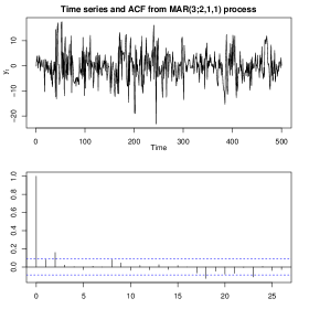
Figure 1: Simulated time series from $\operatorname*{tMAR}(3;2,1,1)$ process (top) and sample autocorrelation.

For the analysis, we compared all possible models with 2 and 3 mixture components, and maximum autoregressive order equal to 4.

For what regards the optimal autoregressive orders, the RJMCMC algorithm chooses a $\operatorname*{tMAR}(3;2,1,1)$ among all 3-component models, with a preference of $0.8054$ (i.e. the model was retained as ”best” 3-component model on roughly $81\%$ of the iterations), and a $\operatorname*{tMAR}(2;2,1)$ among all 2-component models, with a preference of $0.8149$. When compared with each other in terms of marginal likelihood, the best model was $\operatorname*{tMAR}(3;2,1,1)$ with marginal log-likelihood of $-1502.77$ against $-1519.166$ for $\operatorname*{tMAR}(2;2,1)$.

We then simulated a sample of length $100000$ from the posterior distribution of the paramters, after allowing $10000$ burn-in iterations. Results are displayed in Figure 2 and Figure 3.

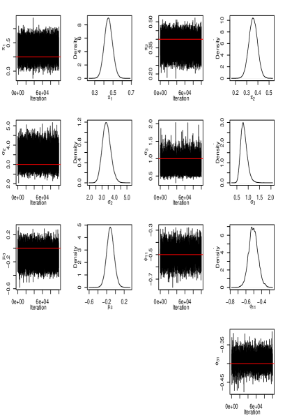
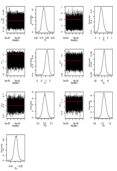
Figure 2: Trace and density plots of full conditional posterior distributions of model parameters under selected $\operatorname*{tMAR}(3;2,1,1)$ model. Red lines highlight true values.

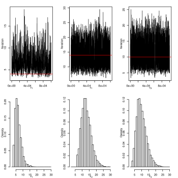
Figure 3: Trace plots and histograms of full conditional posterior distributions of degrees of freedom parameters under selected $\operatorname*{tMAR}(3;2,1,1)$ model, with unit bin-width. Red lines highlight true values.

We can see from Figure 2 that almost all ”true” parameters are included within the $95\%$ posterior density region of their respective distribution. The only exception is found in $\mu_{1}$, for which such region is $[-1.449,-0.0177]$. However, it must be taken into account that component 1 has the largest variance and the largest autoregressive order, and is therefore more subject to sampling variability. For what regards the degrees of freedom parameter, all three components have their peak near the true values of the paramaeters: respectively, peaks are found between $[4,7]$, $[11,13]$ and $[8,11]$ (true values are $4$, $14$ and $10$).

Overall, we may be satisfied with performance of the algorithm.

5 The IBM common stock closing prices

The IBM common stock closing prices (Box and Jenkins, 1976) is a financial time series widely explored several times in the literature, including ravagli2020bayesian, which is our focus for comparison. The series contains 369 observations from May 17th 1961 to November 2nd 1962.

We consider the series of first order differences, which can be seen in Figure 4. The series presents clear signs of heteroskedasticity, therefore a tMAR model may be a reasonable choice to model the data.

Figure 4: Series of first order differences for IBM adjusted closing prices.

For comparison with previous studies, shift parameters $\phi_{k0}$, $k=1,\ldots,g$ are fixed to 0, hence are not paramters in the model. This taken into account, our method chooses a $\operatorname*{tMAR}(2;1,1)$ as best fit among all tMAR models with 2 and 3 mixture components and maximum autoregressive order equal to 4. More specifically, the model was retained about half of the iterations (5067 times over 10000 iterations) by RJMCMC, meaning it is preferred to models with 2 mixing components and larger autoregressive orders. Furthermore, the marginal loglikelihood for this model is $-1232.678$, which is larger than that of the competing $\operatorname*{tMAR}(3;2,1,1)$, $-1258.073$, which was selected as best 3-component model.

Once again, we simulated a sample of size 100000 from the posterior distribution of the parameters, after 10000 burn-in iterations, which can be seen in Figure 5.

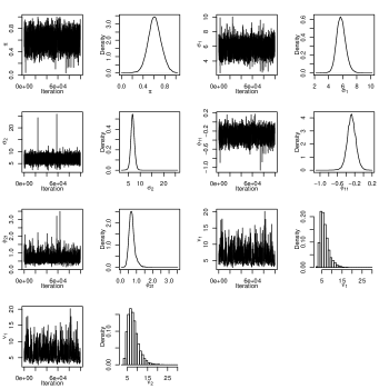
Figure 5: Trace and density plots of parameter posterior distributions under selected $\operatorname*{tMAR}(2;1,1)$ model for the IBM data.

ravagli2020bayesian selected a Gaussian $\operatorname*{MAR}(3;1,1,4)$ as best fit for the same dataset, where one of the mixture components was ”specialised” to model very few observations with large variability. However, the $\operatorname*{tMAR}$ model, thanks to its flexibility in the tails of the distribution, only requires 2 components to account for such noise, returning a model that is simpler, in that it has fewer parameters, and most importantly has a more straightforward interpretation.

6 Conclusions

We have seen a fully Bayesian analysis of mixture autoregressive models with standardised Student t innovations. In a simulation example, it was shown how the method can correctly find the best model to fit a given dataset. In addition, we saw that the proposed MCMC for simulation from parameter posterior distributions quickly converges to stationarity, and that true values of those parameters are found in high density region.

Secondly, we showed the analysis performed on the IBM common stock closing prices, a dataset widely exploited in the literature of heteroskedastic models. In particular, we focused on comparison with the analysis of ravagli2020bayesian here, which used a Gaussian MAR model. Results tell that, thanks to the flexibility of the Student t distribution in its tails, we are able now to fit the data with a considerably more parsimonious model, which also has an easier interpretation.

A limitation of the proposed method is that it inevitably relies on prior information when it comes to degrees of freedom parameters. In practice, this means that if one incorporates wrong prior beliefs, the resulting posterior distribution will be affected, potentially leading to wrong conclusions. One way to make this part of the analysis more objective could be adapting Jeffrey’s priors for the Student t regression model (Fonseca et al., 2008b) to the case of mixture autoregression. However, this would require derivation of the information matrix. On the other hand, the method performs well as long as hyperparameters are set ”loosely” around the true value of the parameter of interest, so that it may worth using as long as prior information is broadly reliable (i.e. it is sufficient that EM-estimates are available).

References

- (1)
- Boshnakov (2011) Boshnakov, G. N.: 2011, On first and second order stationarity of random coefficient models, Linear Algebra Appl. 434(2), 415–423.
- Box and Jenkins (1976) Box, G. E. P. and Jenkins, G. M.: 1976, Time series analysis : forecasting and control / George E.P. Box and Gwilym M. Jenkins, rev. ed. edn, Holden-Day San Francisco.
- Chib (1995) Chib, S.: 1995, Marginal likelihood from the Gibbs output., J. A. Stat. Ass. 90(432), 1313–1321.
- Chib and Jeliazkov (2001) Chib, S. and Jeliazkov, I.: 2001, Marginal likelihood from the Metropolis-Hastings output., J. A. Stat. Ass. 96(453), 270–281.
- Dempster et al. (1977) Dempster, A. P., Laird, N. M. and Rubin, D. B.: 1977, Maximum likelihood from incomplete data via the em algorithm, Journal of the royal statistical society. Series B (methodological) pp. 1–38.
- Diebolt and Robert (1994) Diebolt, J. and Robert, C. P.: 1994, Estimation of finite mixture distributions through bayesian sampling, Journal of the Royal Statistical Society. Series B (Methodological) 56, 363–375.
-
Fonseca et al. (2008a)
Fonseca, T. C. O., Ferreira, M. A. R. and Migon, H. S.: 2008a, Objective
bayesian analysis for the student-t regression model, Biometrika 95(2), 325–333.
http://www.jstor.org/stable/20441467 -
Fonseca et al. (2008b)
Fonseca, T. C. O., Ferreira, M. A. R. and Migon, H. S.: 2008b, Objective
bayesian analysis for the student-t regression model, Biometrika 95(2), 325–333.
http://www.jstor.org/stable/20441467 -
Geweke (1993)
Geweke, J.: 1993, Bayesian treatment of the independent student-t linear model,
Journal of Applied Econometrics 8, S19–S40.
http://www.jstor.org/stable/2285073 - Geweke (1994) Geweke, J.: 1994, Priors for macroeconomic time series and their application, Econometric Theory 10(3-4), 609–632.
- Green (1995) Green, P. J.: 1995, Reversible jump markov chain monte carlo computation and bayesian model determination, Biometrika 82(4), 711–732.
- Richardson and Green (1997) Richardson, S. and Green, P. J.: 1997, On Bayesian Analysis of Mixtures with an Unknown Number of Components., J. R. Stat. Soc., Ser. B, Stat. Methodol. 59(4), 731–792.
- Sampietro (2006) Sampietro, S.: 2006, Bayesian analysis of mixture of autoregressive components with an application to financial market volatility, Applied Stochastic Models in Business and Industry 22(3), 242.
-