Abstract

Higher dimensional closed Friedmann–Lemaître–Robertson–Walker (FLRW) universe with positive cosmological constant is investigated by Regge calculus. A Cauchy surface of discretized FLRW universe is replaced by a regular polytope in accordance with the Collins–Williams (CW) formalism. Polytopes in an arbitrary dimensions can be systematically dealt with by a set of five integers integrating the Schläfli symbol of the polytope. Regge action in continuum time limit is given. It possesses reparameterization invariance of the time variable. Variational principle for edge lengths and struts yields Hamiltonian constraint and evolution equation. They describe oscillating universe in dimensions larger than three. To go beyond the approximation by regular polytopes, we propose pseudo-regular polytopes with fractional Schläfli symbols as a substitute for geodesic domes in higher dimensions. We examine the pseudo-regular polytope model as an effective theory of Regge calculus for the geodesic domes. In the infinite frequency limit, the pseudo-regular polytope model reduces to the continuum FLRW universe.

1 Introduction

Regge calculus is a coordinate free geometric formalism of gravitation on triangulated piecewise linear manifolds [1, 2]. It is envisaged from classical to quantum as an approach of Einstein gravity to problems where analytic methods cannot be reachable. Though Regge theory or its evolved ones have brought considerable progress in our understanding of quantum gravity, in particular in two and three dimensions, efforts to develop the formalism are vigorously continued to overcome the conceptual and technical difficulties [3].

As in continuum gravity, Regge calculus allows exact solutions for systems, where the numbers of variables are largely reduced by some symmetry. They are expected not only to play a role of a test tube to examine the validity of Regge calculus but to expose origins of intriguing geometrical properties of gravitation such as dynamical behaviors of space-time and black hole singularities. Along this line of thought Regge calculus has been applied to spherically symmetric static geometries such as the Schwarzschild space-time [4] and the Friedmann–Lemaître–Robertson–Walker (FLRW) universe [5, 6, 7, 8, 9]. Most researches assume realistic four dimensions and application of Regge calculus to higher dimensions have not been targeted so far.

In this paper we investigate vacuum solution of a discretized closed FLRW universe with a positive cosmological constant in an arbitrary dimensions via Regge calculus. In the previous papers [10, 11] we have analyzed the FLRW universe in three and four dimensions within the framework of Collins–Williams (CW) formalism[5]. It is base on $3+1$ decomposition of space-time similar to Arnowitt–Deser–Misner (ADM) formalism in General Relativity [12, 13]. Three-dimensional spherical Cauchy surfaces are replaced by regular polytopes and truncated world-tubes are taken as the fundamental building blocks of the discretized FLRW universe. Regge calculus describes qualitative properties of the continuum solution during the period small enough compared with the characteristic time scale $\sim 1/\sqrt{\Lambda}$, the inverse square root of the cosmological constant. The deviation from the continuum theory becomes apparent as time passes. In three dimensions the universe expands to infinity in a finite time, whereas it repeats expansions and contractions periodically in four dimensions.

In order for Regge calculus to approximate continuum theory quantitatively edge lengths must be sufficiently small compared both with the curvature radius and $1/\sqrt{\Lambda}$. This cannot be satisfied for regular polytopes since the edge lengths and their circumradii are of same order, and the minimum edge lengths are of order $1/\sqrt{\Lambda}$. To improve the approximation we must introduce nonregular polytopes with shorter edge lengths. A natural construction of such polytopes is geodesic dome. Regge calculus for them, however, becomes impractical as the number of cells increases. This can be bypassed by working with the pseudo-regular polytopes introduced in [10, 11]. They can be simply defined by extending the Schläfli symbol of the original regular polytope to fractional or noninteger one corresponding to the geodesic dome. We will extend the results obtained in three and four dimensions to arbitrary dimensions.

This paper is organized as follows; in the next section we set up the regular polytopal universe by the CW formalism in arbitrary dimensions and formulate the Regge action in the continuum time limit. In Sect. 3 we give gauge fixed Regge equations in Lorentzian signature. We describe the evolution of the polytopal universe in detail. Comparison with the continuum solutions is made. In Sect. 4 we consider the pseudo-regular polytope having a $D$-cube as the parent regular polytope and define the fractional Schläfli symbol. Taking the infinite frequency limit, we argue that the pseudo-regular polytope model can reproduce the continuum FLRW universe. Sect. 5 is devoted to summary and discussions. In Appendix A, we describe circumradii and dihedral angles of regular polytopes in arbitrary dimensions. Appendices B and C are to explain some technicalities.

2 Regge action for a regular $D$-polytopal universe

In the beginning we would like to briefly summarize the FLRW universe in General Relativity. The continuum gravitational action with a cosmological constant in $D$ dimensions is given by

$$S=\frac{1}{16\pi}\int d^{D}x\sqrt{-g}(R-2\Lambda).$$ (2.1)

The FLRW metric

$$ds^{2}=-dt^{2}+a(t)^{2}\left[\frac{dr^{2}}{1-kr^{2}}+r^{2}\sigma_{AB}dx^{A}dx^{B}\right]$$ (2.2)

is an exact solution of Einstein’s field equations, where $\sigma_{AB}$ is the metric tensor on $(D-2)$-dimensional unit sphere. It describes an expanding or contracting universe of homogeneous and isotropic space. All the time dependence of the metric is included in $a\left(t\right)$, known as scale factor in cosmology. Einstein equations for the metric (2.2) derive the Friedmann equations as differential equations of scale factor

$$\ddot{a}=\Lambda_{D}a,\quad\dot{a}^{2}=\Lambda_{D}a^{2}-k,$$ (2.3)

where we have introduced $\Lambda_{D}$ by

$$\Lambda_{D}=\frac{2\Lambda}{\left(D-1\right)\left(D-2\right)}.$$ (2.4)

The curvature parameter $k=1,0,-1$ corresponds to space being spherical, Euclidean, or hyperbolic, respectively. The relations between the solutions and curvature parameter are summarized in Table 1 with the proviso that the behaviors of the universes are restricted to expanding at the beginning for the initial condition $a\left(0\right)=\min a\left(t\right)$. Note that we have assumed $a(0)=\frac{1}{\sqrt{\Lambda_{D}}}$ for the case of $k=0$ and $\Lambda>0$.

$$\begin{array}[]{cccc}\hline\cr&k=1&k=0&k=-1\\ \hline\cr\Lambda>0&a=\frac{1}{\sqrt{\Lambda_{D}}}\cosh\left(\sqrt{\Lambda_{D}}t\right)&a=\frac{1}{\sqrt{\Lambda_{D}}}\exp\left(\sqrt{\Lambda_{D}}t\right)&a=\frac{1}{\sqrt{\Lambda_{D}}}\sinh\left(\sqrt{\Lambda_{D}}t\right)\\ \Lambda=0&\mbox{no solution}&a=\mbox{const.}&a=t\\ \Lambda<0&\mbox{no solution}&\mbox{no solution}&a=\frac{1}{\sqrt{-\Lambda_{D}}}\sin\left(\sqrt{-\Lambda_{D}}t\right)\\ \hline\cr\end{array}$$

Table 1: Solutions of the Friedmann equations.

	Name	$\left\{p_{1},p_{2},p_{3},\cdots,p_{D},p_{0}\right\}$	$[D,\kappa_{D},\lambda_{D},\mu_{D},\zeta_{D}]$
0-polytope	Point	$\left\{2\right\}$	$[0,3,3,3,3]$
1-polytope	Line segment	$\left\{2,2\right\}$	$[1,3,3,3,3]$
2-polytope	$n$-sided polygon	$\left\{2,n,2\right\}$	$[2,n,3,3,3]$
3-polytope	Tetrahedron	$\left\{2,3,3,2\right\}$	$[3,3,3,3,3]$
	Cube	$\left\{2,4,3,2\right\}$	$[3,4,3,3,3]$
	Octahedron	$\left\{2,3,4,2\right\}$	$[3,3,4,3,3]$
	Dodecahedron	$\left\{2,5,3,2\right\}$	$[3,5,3,3,3]$
	Icosahedron	$\left\{2,3,5,2\right\}$	$[3,3,5,3,3]$
4-polytope	5-cell	$\left\{2,3,3,3,2\right\}$	$[4,3,3,3,3]$
	8-cell	$\left\{2,4,3,3,2\right\}$	$[4,4,3,3,3]$
	16-cell	$\left\{2,3,3,4,2\right\}$	$[4,3,3,4,3]$
	24-cell	$\left\{2,3,4,3,2\right\}$	$[4,3,4,3,3]$
	120-cell	$\left\{2,5,3,3,2\right\}$	$[4,5,3,3,3]$
	600-cell	$\left\{2,3,3,5,2\right\}$	$[4,3,3,5,3]$
$n$-polytope $\left(n\geq 5\right)$	$n$-simplex $\alpha_{n}$	$\left\{2,3^{n-1},2\right\}$	$[n,3,3,3,3]$
	$n$-orthoplex $\beta_{n}$	$\left\{2,3^{n-2},4,2\right\}$	$[n,3,3,3,4]$
	$n$-cube $\gamma_{n}$	$\left\{2,4,3^{n-2},2\right\}$	$[n,4,3,3,3]$

Table 2: Extended Schläfli symbols for regular polytopes. The symbol $\{2,3^{4},2\}$ is an abbreviation of $\{2,3,3,3,3,2\}$. By H. M. S. Coxeter the $n$-simplex, $n$-orthoplex, and $n$-cube are labeled as $\alpha_{n}$, $\beta_{n}$, and $\gamma_{n}$, respectively [17]. The parameter set $\left[D,\kappa_{D},\lambda_{D},\mu_{D},\zeta_{D}\right]$ is another way to specify a regular $D$-polytope introduced in Sect. 3.

As preparation for the investigation of polytopal universes, we work in Euclidean space-time for the time being and explain an epitome of Regge calculus; in Regge calculus, the discrete gravitational action is given by the Regge action[14]

$$S_{\rm Regge}=\frac{1}{8\pi}\left(\sum_{i\in\rm\{hinges\}}\varepsilon_{i}A_{i}-\Lambda\sum_{i\in\rm\{blocks\}}V_{i}\right),$$ (2.5)

where $A_{i}$ is the volume of a hinge, $\varepsilon_{i}$ the deficit angle around the hinge of volume $A_{i}$, and $V_{i}$ the volume of a building block of the piecewise linear manifold. The fundamental variables in Regge calculus are the edge lengths $l_{i}$. Varying the Regge action with respect to $l_{i}$, we obtain the Regge equations

$$\sum_{i\in\rm\{hinges\}}\varepsilon_{i}\frac{\partial A_{i}}{\partial l_{j}}-\Lambda\sum_{i\in\rm\{blocks\}}\frac{\partial V_{i}}{\partial l_{j}}=0.$$ (2.6)

Note that there is no need to carry out the variation of the deficit angle owing to the Schläfli identity[15, 16]

$$\sum_{i\in\rm\{hinges\}}A_{i}\frac{\partial\varepsilon_{i}}{\partial l_{j}}=0.$$ (2.7)

We now turn to polytopal universe. According to CW formalism we replace $(D-1)$-dimensional hyperspherical Cauchy surface in FLRW universe by a fixed type of regular $D$-polytope. In general a regular $D$-polytope for $D\geq 2$ is characterized by a set of $D-1$ integer parameters $\left\{p_{2},p_{3},\cdots,p_{D}\right\}$, known as Schläfli symbol[17, 18]. In this paper we introduce $p_{0}=p_{1}=2$ to include the cases of $D=0,~{}1$ and write the Schläfli symbol as $\left\{p_{1},p_{2},p_{3}\cdots,p_{D},p_{0}\right\}$, which will be referred to as extended Schläfli symbol. Each regular $D$-polytope has a corresponding dual polytope represented by the extended Schläfli symbol in reverse order $\left\{p_{0},p_{n},p_{n-1},\cdots,p_{1}\right\}$. Note that there are only three types of regular polytopes in dimensions larger than four: the $n$-simplex, $n$-orthoplex, and $n$-cube being, respectively, higher dimensional analogs of the tetrahedron, octahedron, and cube in three dimensions. In Table 2[11] we summarize all possible regular polytopes in arbitrary dimensions.

Figure 1: The $i$-th frustum as the fundamental building block of the 5-polytopal universe for $\left\{2,3^{4},2\right\}$. A lower cell like ABCDE for $\left\{2,3,3,3,2\right\}$ with edge length $l_{i}$ at the time $t_{i}$ evolves into an upper one A^↑B^↑C^↑D^↑E^↑ with $l_{i+1}$ at $t_{i+1}$. The 3-frustum ABC-A^↑B^↑C^↑ having 2-simplices $\left\{2,3,2\right\}$ as base faces is a temporal hinge, and the 3-simplex ABCD for $\left\{2,3,3,2\right\}$ a spatial hinge.

In the present polytopal universe the fundamental building blocks of space-time are world-tubes of $D$-dimensional frustums with the regular $(D-1)$-polytopes $\left\{p_{1},\cdots,p_{D-1},p_{0}\right\}$ as the upper and lower cells. We will refer to them as $D$-frustums. In Figure 1 we give, as an illustration, a depiction of a 5-frustum with 4-simplices as base cells. We assume that the upper and lower cells of a block lie in two consecutive time-slices separately and every strut between them has equal length. We denote the volume of the $i$-th $D$-frustum by $V_{i}$. It contains two types of the fundamental variables: the edge lengths $l_{i}$ and $l_{i+1}$ of the lower and upper $(D-1)$-polytopes, and the lengths of the struts $m_{i}$. In a $D$-dimensional piecewise linear manifold, hinges are ($D-2$)-dimensional objects, where curvature is concentrated. There are two types of hinges. One is temporally extended $(D-2)$-frustums with regular $(D-3)$-polytopes $\left\{p_{1},\cdots,p_{D-3},p_{0}\right\}$ as the base cells, like the frustum $\mathrm{ABC\hbox{-}A}^{\uparrow}\mathrm{B}^{\uparrow}\mathrm{C}^{\uparrow}$ in Figure 1. We call them “temporal hinges” and denote by $A_{i}^{({\rm t})}$ the volume of a temporal hinge between the $i$-th and $(i+1)$-th Cauchy surfaces. The other is spatially traversed regular $(D-2)$-polytopes $\left\{p_{1},\cdots,p_{D-2},p_{0}\right\}$ as facets of a Cauchy cell, or equivalently ridges of Cauchy surface, such as $\mathrm{ABCD}$. Note that in geometry a $(D-1)$-, $(D-2)$-, and $(D-3)$-dimensional face of $D$-polytope are also called a facet, ridge, and peak, respectively. We call the codimension two polytopes “spatial hinges” and denote by $A_{i}^{({\rm s})}$ the volume of the hinge lying in the $i$-th time-slice.

We are able to write the Regge action for the polytopal universe by counting the numbers of temporal hinges lying between two consecutive time-slices, spatial hinges in a time-slice, and $D$-frustums. They are just the numbers of peaks, ridges, and facets of the $D$-polytope, respectively. Let $N^{(D)}_{n}$ be the number of $n$-dimensional faces of a regular $D$-polytope, then the Regge action (2.5) can be written as

$$S_{\mathrm{Regge}}=\frac{1}{8\pi}\sum_{i}\left(N^{(D)}_{D-3}A^{({\rm t})}_{i}\varepsilon_{i}^{\rm(t)}+N^{(D)}_{D-2}A^{({\rm s})}_{i}\varepsilon_{i}^{\rm(s)}-N^{(D)}_{D-1}\Lambda V_{i}\right),$$ (2.8)

where $\varepsilon^{\rm({\rm t})}_{i}$ and $\varepsilon_{i}^{\rm({\rm s})}$ are the deficit angles around a temporal hinge of volume $A_{i}^{(\rm t)}$ and a spatial hinge of volume $A_{i}^{(\rm s)}$, respectively. The summation is taken over the time-slices. The volume of the frustum, those of hinges, and deficit angles can be expressed in terms of the fundamental variables $l$’s and $m$’s.

For the purpose it is convenient to introduce the circumradius $\hat{R}_{n}$ and volume $\hat{\cal V}^{(n)}$ of a regular $n$-polytope $\Pi_{n}=\{p_{1},p_{2},\cdots,p_{n},p_{0}\}$ with unit edge length. In Appendix A we give a general formula for $\hat{R}_{n}$. See (A.1) and (A.4). The normalized volume $\hat{\cal V}^{(n)}$ can be obtained from the recurrence relation

$$\hat{\cal{V}}^{(n)}=\frac{N^{(n)}_{n-1}\sqrt{\hat{R}_{n}^{2}-\hat{R}_{n-1}^{2}}}{n}\hat{\cal{V}}^{(n-1)},\quad\hat{\cal{V}}^{(0)}=1,$$ (2.9)

where $\hat{R}_{0}=0$ is assumed. It is now straightforward to write the volumes $V_{i}$ and $A_{i}^{(\mathrm{s,t})}$ as

$$V_{i} =\frac{1}{D}\hat{\cal{V}}^{(D-1)}\sqrt{m_{i}^{2}-\hat{R}_{D-1}^{2}\delta l_{i}^{2}}\frac{l^{D}_{i+1}-l^{D}_{i}}{l_{i+1}-l_{i}},$$ (2.10)

$$A_{i}^{({\rm s})} =\hat{\cal{V}}^{(D-2)}l_{i}^{D-2},$$ (2.11)

$$A_{i}^{({\rm t})} =\frac{1}{D-2}\hat{\cal{V}}^{(D-3)}\sqrt{m_{i}^{2}-\hat{R}_{D-3}^{2}\delta l_{i}^{2}}\frac{l^{D-2}_{i+1}-l^{D-2}_{i}}{l_{i+1}-l_{i}},$$ (2.12)

where we have introduced the difference of edge length $\delta l_{i}=l_{i+1}-l_{i}$.

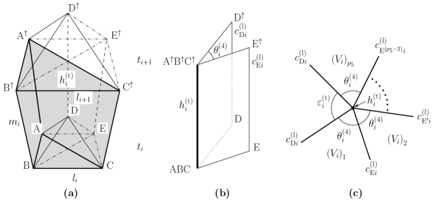
Figure 2: (a) Two lateral cells $c^{(\rm l)}_{{\rm D}i}$ and $c^{(\rm l)}_{{\rm E}i}$ are meeting at a temporal hinge $h^{(\rm t)}_{i}$, (b) $\theta^{(4)}_{i}$ is the dihedral angle between these cells, and (c) $\varepsilon^{(\rm t)}_{i}$ the deficit angle around the hinge $h^{(\rm t)}_{i}$ made by $p_{5}$ frustums $\left(V_{i}\right)_{1},\cdots,\left(V_{i}\right)_{p_{5}}$ having $h^{(\rm t)}_{i}$ as a lateral cell in common.

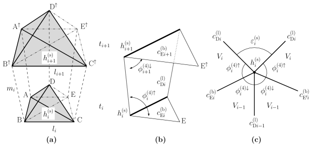
Figure 3: (a) Two spatial hinges $h^{(\rm s)}_{i}$ and $h^{(\rm s)}_{i+1}$ in the $i$-th frustum, (b) dihedral angles $\phi^{(4)\uparrow}_{i}$ and $\phi^{(4)\downarrow}_{i+1}$, and (c) deficit angle $\varepsilon^{(\rm s)}_{i}$.

To find the deficit angle around a hinge we need a dihedral angle between two adjacent cells jointed at the hinge. As an example consider the hinges of a 5-frustum with regular 4-polytopal bases as laid out in Figure 1. At the temporal hinge $h^{(\rm t)}_{i}=\mathrm{ABC\hbox{-}A^{\uparrow}B^{\uparrow}C^{\uparrow}}$ in Figure 2, the dihedral angle $\theta^{(4)}_{i}$ is made by two lateral cells $c^{(\rm l)}_{{\rm D}i}=\mathrm{ABCD\hbox{-}A^{\uparrow}B^{\uparrow}C^{\uparrow}D^{\uparrow}}$ and $c^{(\rm l)}_{{\rm E}i}=\mathrm{ABCE\hbox{-}A^{\uparrow}B^{\uparrow}C^{\uparrow}E^{\uparrow}}$. On the other hand, $\phi^{(4)\uparrow}_{i}$ is the dihedral angle at the hinge $h^{(\rm s)}_{i}=\mathrm{ABCD}$ between the lateral cell $c^{(\rm l)}_{{\rm D}i}$ and the lower base cell $c^{(\rm b)}_{{\rm E}i}=\mathrm{ABCDE}$ as illustrated in Figure 3, and similarly $\phi^{(4)\downarrow}_{i+1}$ the one between $c^{(\rm l)}_{{\rm D}i}$ and $c^{(\rm b)}_{{\rm E}i+1}=\mathrm{A^{\uparrow}B^{\uparrow}C^{\uparrow}D^{\uparrow}E^{\uparrow}}$ at $h^{(\rm s)}_{i+1}=\mathrm{A^{\uparrow}B^{\uparrow}C^{\uparrow}D^{\uparrow}}$. For a $D$-frustum with $(D-1)$-polytopal bases, the dihedral angles $\theta^{(D-1)}_{i}$ and $\phi^{(D-1)\downarrow}_{i+1}$ can be written as

$$\theta_{i}^{(D-1)} =2\arccos\left[\sqrt{\frac{m_{i}^{2}-\hat{R}^{2}_{D-1}\delta l_{i}^{2}}{m_{i}^{2}-\hat{R}^{2}_{D-2}\delta l_{i}^{2}}}\cos\frac{\vartheta_{D-1}}{2}\right],$$ (2.13)

$$\phi_{i+1}^{(D-1)\downarrow} =\arccos\left[\sqrt{\frac{\hat{R}^{2}_{D-1}-\hat{R}_{D-2}^{2}}{m_{i}^{2}-\hat{R}^{2}_{D-2}\delta l_{i}^{2}}}\>\delta l_{i}\right],$$ (2.14)

where $\vartheta_{n}$ is the dihedral angle of a regular $n$-polytope $\Pi_{n}$. Since the upper cell of the $D$-frustum is parallel to the lower, $\phi^{(D-1)\uparrow}_{i}$ and $\phi^{(D-1)\downarrow}_{i+1}$ satisfy

$$\phi^{(D-1)\uparrow}_{i}+\phi^{(D-1)\downarrow}_{i+1}=\pi.$$ (2.15)

In Appendix A we give a short account of dihedral angles of regular polytopes. Derivations of (2.13) and (2.14) are given in Appendix B.

Taking it into the consideration that $p_{D}$ frustums have a temporal hinge in common as in Figure 2(c), the deficit angle $\varepsilon_{i}^{({\rm t})}$ is given by

$$\varepsilon_{i}^{({\rm t})}=2\pi-p_{D}\theta_{i}^{(D-1)}.$$ (2.16)

On the other hand the spatial hinge $h^{(\rm s)}_{i}$ is always shared by four frustums as illustrated in Figure 3(c): two adjacent blocks of volume $V_{i}$ in the future side and two $V_{i-1}$ in the past side. Thus the deficit angle $\varepsilon_{i}^{({\rm s})}$ is expressed as

$$\varepsilon_{i}^{({\rm s})}=2\pi-2\left(\phi_{i}^{(D-1)\uparrow}+\phi_{i}^{(D-1)\downarrow}\right)=2\delta\phi_{i}^{(D-1)\downarrow},$$ (2.17)

where $\delta\phi_{i}^{(D-1)\downarrow}=\phi_{i+1}^{(D-1)\downarrow}-\phi_{i}^{(D-1)\downarrow}$.

A facet of regular $D$-polytope is a $(D-1)$-polytope having $N^{(D-1)}_{D-2}$ ridges of the $D$-polytope and a ridge is shared by two facets, so that $N^{(D)}_{D-1}$, $N^{(D-1)}_{D-2}$, and $N^{(D)}_{D-2}$ satisfy $N^{(D-1)}_{D-2}N^{(D)}_{D-1}=2N^{(D)}_{D-2}$. Likewise, a ridge has $N^{(D-2)}_{D-3}$ peaks of the $D$-polytope and a peak joints two ridges in a facet, so a facet has $\dfrac{N^{(D-1)}_{D-2}N^{(D-2)}_{D-3}}{2}$ peaks. Taking it into account of the fact that a peak connects $p_{D}$ facets, we find a relation $\dfrac{N^{(D-1)}_{D-2}N^{(D-2)}_{D-3}}{2}N^{(D)}_{D-1}=p_{D}N^{(D)}_{D-3}$. These constraints together with (2.9) lead to

$$\frac{N^{(D)}_{D-2}\hat{\cal V}^{(D-2)}}{N^{(D)}_{D-3}\hat{\cal V}^{(D-3)}}= \frac{p_{D}}{D-2}\sqrt{\hat{R}_{D-2}^{2}-\hat{R}_{D-3}^{2}},$$ (2.18)

$$\frac{N^{(D)}_{D-1}\hat{\cal V}^{(D-1)}}{N^{(D)}_{D-3}\hat{\cal V}^{(D-3)}}= \frac{2p_{D}}{(D-1)(D-2)}\sqrt{(\hat{R}_{D-1}^{2}-\hat{R}_{D-2}^{2})(\hat{R}_{D-2}^{2}-\hat{R}_{D-3}^{2})}$$

$$= \frac{2p_{D}}{(D-1)(D-2)}(\hat{R}_{D-2}^{2}-\hat{R}_{D-3}^{2})\tan\frac{\vartheta_{D-1}}{2},$$ (2.19)

which can be used to factor out the three couplings appearing in the action (2.8). As for the second equality in (2), use has been made of (A.23). We thus obtain

$$S_{\mathrm{Regge}}= \frac{N^{(D)}_{D-3}\hat{\cal{V}}^{(D-3)}}{8\pi}\sum_{i}\Biggl{(}\frac{1}{D-2}\sqrt{m_{i}^{2}-\hat{R}_{D-3}^{2}\delta l_{i}^{2}}\frac{l^{D-2}_{i+1}-l^{D-2}_{i}}{l_{i+1}-l_{i}}\varepsilon_{i}^{\rm(t)}$$

$$+\frac{2p_{D}}{D-2}\sqrt{\hat{R}_{D-2}^{2}-\hat{R}_{D-3}^{2}}l_{i}^{D-2}\delta\phi_{i}^{(D-1)\downarrow}$$

$$-\frac{p_{D}\Lambda_{D}}{D}(\hat{R}_{D-2}^{2}-\hat{R}_{D-3}^{2})\sqrt{m_{i}^{2}-\hat{R}_{D-1}^{2}\delta l_{i}^{2}}\frac{l^{D}_{i+1}-l^{D}_{i}}{l_{i+1}-l_{i}}\tan\frac{\vartheta_{D-1}}{2}\Biggr{)}.$$ (2.20)

In later sections we are interested in the continuum time limit. We replace $l_{i}$ and $m_{i}$ by $l(\tau)$ and $n(\tau)\delta\tau$, where $\tau$ is an arbitrary parameter and $n(\tau)$ can be regarded as lapse function in ADM formalism. The continuum limit $\delta\tau\rightarrow d\tau$ of the action can easily be obtained from (2) as

$$S_{\mathrm{Regge}}= \frac{N^{(D)}_{D-3}\hat{\cal{V}}^{(D-3)}}{8\pi}\int d\tau\Biggl{(}\sqrt{n^{2}-\hat{R}_{D-3}^{2}\dot{l}^{2}}\>l^{D-3}\varepsilon^{\rm(t)}-2p_{D}\sqrt{\hat{R}_{D-2}^{2}-\hat{R}_{D-3}^{2}}\>l^{D-3}\dot{l}\phi^{(D-1)\downarrow}$$

$$-p_{D}\Lambda_{D}(\hat{R}_{D-2}^{2}-\hat{R}_{D-3}^{2})\sqrt{n^{2}-\hat{R}_{D-1}^{2}\dot{l}^{2}}\>l^{D-1}\tan\frac{\vartheta_{D-1}}{2}\Biggr{)},$$ (2.21)

where $\dot{l}=\dfrac{dl}{d\tau}$ and total $\tau$ derivative terms are suppressed. We have also introduced continuum limits of (2.13), (2.14), and (2.16) by

$$\varepsilon^{(\mathrm{t})} =2\pi-p_{D}\theta^{(D-1)}\quad\hbox{with}\quad\theta^{(D-1)}=2\arccos\left[\sqrt{\frac{n^{2}-\hat{R}^{2}_{D-1}\dot{l}^{2}}{n^{2}-\hat{R}^{2}_{D-2}\dot{l}^{2}}}\cos\frac{\vartheta_{D-1}}{2}\right],$$ (2.22)

$$\phi^{(D-1)\downarrow} =\arccos\left[\sqrt{\frac{\hat{R}^{2}_{D-1}-\hat{R}_{D-2}^{2}}{n^{2}-\hat{R}^{2}_{D-2}\dot{l}_{i}^{2}}}\>\dot{l}\right].$$ (2.23)

The Regge action (2) is invariant under an arbitrary reparameterization

$$\tau\to\tau^{\prime}=f(\tau),\quad n(\tau)\to n^{\prime}(\tau^{\prime})=\frac{n(\tau)}{\dot{f}(\tau)},\quad l(\tau)\to l^{\prime}(\tau^{\prime})=l(\tau).$$ (2.24)

This can be used to fix the lapse function.

3 Regge equations

The Regge equations can be obtained by taking variations of the Regge action with respect to $n$ and $l$. The equations of motion possess the local symmetry (2.24). We must fix it by imposing some condition on the dynamical variables. Furthermore, the action is based on the piecewise linear manifold with Euclidean signature. We must carry out inverse Wick rotation to recover Lorentzian signature. As for fixing the local invariance we impose the following gauge condition on the lapse function

$$n(\tau)=1.$$ (3.1)

We then carry out inverse Wick rotation by $\tau=it$, where $t$ can be regarded as the time of a clock fixed at a vertex of the polytopal universe. The time axis is taken to be parallel to a strut. It is not orthogonal to Cauchy cells. If we consider nonregular polytopes with shorter edge lengths and more cells such as geodesic domes [10], we would have a better approximation of a smooth hypersphere. The orthogonality of the time axis with the spatial ones as in the FLRW universe can be restored in the limit of smooth hypersphere. We thus obtain the Regge equations

$$2\pi-p_{D}\theta^{(D-1)}=p_{D}\Lambda_{D}(\hat{R}_{D-2}^{2}-\hat{R}_{D-3}^{2})\sqrt{\frac{1+\hat{R}_{D-3}^{2}\dot{l}^{2}}{1+\hat{R}_{D-1}^{2}\dot{l}^{2}}}\>l^{2}\tan\frac{\vartheta_{D-1}}{2},$$ (3.2)

$$\frac{\ddot{l}}{1+\hat{R}_{D-2}^{2}\dot{l}^{2}}=\Lambda_{D}l\left[1+\hat{R}_{D-3}^{2}\dot{l}^{2}-\frac{(\hat{R}_{D-1}^{2}-\hat{R}_{D-3}^{2})l\ddot{l}}{2(1+\hat{R}_{D-1}^{2}\dot{l}^{2})}\right],$$ (3.3)

where the dots on $l$ stand for $t$ derivatives and $\theta^{(D-1)}$ in lorentzian signature is given by

$$\theta^{(D-1)}=2\arccos\left[\sqrt{\frac{1+\hat{R}^{2}_{D-1}\dot{l}^{2}}{1+\hat{R}^{2}_{D-2}\dot{l}^{2}}}\cos\frac{\vartheta_{D-1}}{2}\right].$$ (3.4)

Eq. (3.2) is known as the Hamiltonian constraint in ADM formalism of canonical General Relativity. The equation of motion for $l$ is referred to as the evolution equation. We have simplified the evolution equation by using the Hamiltonian constraint. It is straightforward to show that the evolution equation can be obtained as the consistency of the Hamiltonian constraint with the time-development. We also mention that (3.2) and (3.3) reproduce the results of Refs. [10, 11] in three and four dimensions.

It is convenient to express the solution to the Regge equations in terms of the dihedral angle $\theta=\theta^{(D-1)}$. Solving (3.2) and (3.4) with respect to $l^{2}$ and $\dot{l}^{2}$, we obtain

$$l= \sqrt{\frac{(2\pi-p_{D}\theta)\cot\frac{\theta}{2}}{p_{D}\Lambda_{D}(\hat{R}_{D-2}^{2}-\hat{R}_{D-3}^{2})}},$$ (3.5)

$$\dot{l}= \pm\frac{1}{\hat{R}_{D-2}}\sqrt{\frac{\cos\theta-\cos\theta_{0}}{\cos\theta_{\mathrm{c}}-\cos\theta}},$$ (3.6)

where $\theta_{0}=\vartheta_{D-1}$ stands for the dihedral angle of a Cauchy cell $\left\{p_{1},p_{2},\cdots,p_{D-1},p_{0}\right\}$ and determines the minimum size of the universe. $\theta_{\mathrm{c}}$ is defined by

$$\theta_{\mathrm{c}}=2\arcsin\left[\frac{\hat{R}_{D-3}}{\hat{R}_{D-2}}\sin\frac{\vartheta_{D-1}}{2}\right].$$ (3.7)

The velocity $\dot{l}$ diverges for $\theta=\theta_{\mathrm{c}}$, where the edge length becomes maximum. In three dimensions $\theta_{\mathrm{c}}=0$ since $\hat{R}_{0}=0$. It matches $\vartheta_{1}$ the dihedral angle of a 1-polytope $\left\{p_{1},p_{0}\right\}$. See (A.21). In dimensions larger than three $\theta_{\mathrm{c}}$ equals a dihedral angle of a regular polytope corresponding to extended Schläfli symbol $\{p_{1},p_{3},\cdots,p_{D-1},p_{0}\}$, which is a vertex figure of a Cauchy cell. For the vertex figure, see Appendix A.

Eliminating $l$ from (3.5) and (3.6), we can derive the differential equation for $\theta$

$$\dot{\theta} =\mp\frac{2\sqrt{p_{D}\Lambda_{D}(2\pi-p_{D}\theta)\sin\theta}}{2\pi-p_{D}(\theta-\sin\theta)}\frac{\sin\frac{\theta}{2}}{\sin\frac{\theta_{0}}{2}}\sqrt{\frac{(\cos\theta_{\mathrm{c}}-\cos\theta_{0})(\cos\theta-\cos\theta_{0})}{\cos\theta_{\mathrm{c}}-\cos\theta}}.$$ (3.8)

The upper sign corresponds to expanding universe and the lower to shrinking one. This leads to an integral representation

$$t\left(\theta\right)=\pm\frac{1}{2\sqrt{p_{D}\Lambda_{D}}}\int_{\theta}^{\theta_{0}}du\frac{2\pi-p_{D}(u-\sin u)}{\sqrt{(2\pi-p_{D}u)\sin u}}\frac{\sin\frac{\theta_{0}}{2}}{\sin\frac{u}{2}}\sqrt{\frac{\cos\theta_{\mathrm{c}}-\cos u}{(\cos\theta_{\mathrm{c}}-\cos\theta_{0})(\cos u-\cos\theta_{0})}},$$ (3.9)

where $\theta_{\mathrm{c}}\leq\theta\leq\theta_{0}$. We have assumed the initial condition

$$\theta(0)=\theta_{0}.$$ (3.10)

As a function of $t$, the dihedral angle $\theta$ is even and monotonically decreasing from $\theta_{0}$ to $\theta_{\mathrm{c}}$ for $0\leq t\leq\tau_{\mathrm{p}}/2$, where $\tau_{\mathrm{p}}$ is given by $\tau_{\mathrm{p}}=2t(\theta_{\mathrm{c}})$. We can extend $\theta(t)$ as a continuous periodic function for arbitrary $t$ by

$$\theta(t+\tau_{\mathrm{p}})=\theta(t).$$ (3.11)

The edge length (3.5) is also a periodic function of $t$. It is continuous for $D\geq 4$, while $l$ diverges for $\theta\left(\tau_{\mathrm{p}}/2\right)=\theta_{\mathrm{c}}=0$ in three dimensions. Note that $\dot{l}/l$ not only diverges but also has a discontinuity at $t=\pm\tau_{\mathrm{p}}/2,~{}\pm 3\tau_{\mathrm{p}}/2,~{}\cdots$. At present it is only an assumption that the polytopal universe in four or more dimensions jumps from expansion to contraction when it reaches the maximum size.

In dimensions larger than four there are only three types of regular polytopes. As can easily be seen from Table 2 any regular polytope can be characterized by $p_{2}$, $p_{3}$, $p_{D}$, and $D$. It is possible to write the circumradii $\hat{R}_{D-k}$ ($k=1,2,3$) and dihedral angles $\vartheta_{D-1}$ appearing in (3.2)–(3.4) in more tractable forms by noting (A.26) and (A.27). To this end we define a set of parameters $\kappa_{n}$, $\lambda_{n}$, $\mu_{n}$, and $\zeta_{n}$ by

$$\kappa_{n} =3\sum_{j=0}^{1}\delta_{j,n}+p_{2}\sum_{j=2}^{\infty}\delta_{j,n},$$ (3.12)

$$\lambda_{n} =3\sum_{j=0}^{2}\delta_{j,n}+p_{3}\sum_{j=3}^{\infty}\delta_{j,n},$$ (3.13)

$$\mu_{n} =3\sum_{j=0}^{3}\delta_{j,n}+p_{4}\sum_{j=4}^{\infty}\delta_{j,n},$$ (3.14)

$$\zeta_{n} =3\sum_{j=0}^{4}\delta_{j,n}+p_{n}\sum_{j=5}^{\infty}\delta_{j,n},$$ (3.15)

where $\delta_{j,k}$ is the Kronecker delta. Obviously, $\kappa_{n}=p_{2}$, $\lambda_{n}=p_{3}$, $\mu_{n}=p_{4}$, and $\zeta_{n}=p_{n}$ for $n\geq 5$. We assign a regular $D$-polytope to a set of five parameters $\left[D,\kappa_{D},\lambda_{D},\mu_{D},\zeta_{D}\right]$. In Table 2 we summarize the correspondence between regular polytopes and the symbol $\left[D,\kappa_{D},\lambda_{D},\mu_{D},\zeta_{D}\right]$. This allows us to express the normalized circumradius $\hat{R}_{D}$ and the dihedral angle $\vartheta_{D}$ in the closed forms as

$$\hat{R}_{D} =\frac{1}{2}\sqrt{\frac{\left[1-\left(D-4\right)\cos\frac{2\pi}{\zeta_{D}}\right]\sin^{2}\frac{\pi}{\lambda_{D}}-2\left[1-\left(D-5\right)\cos\frac{2\pi}{\zeta_{D}}\right]\cos^{2}\frac{\pi}{\mu_{D}}}{\left[1-\left(D-4\right)\cos\frac{2\pi}{\zeta_{D}}\right]\left(\sin^{2}\frac{\pi}{\lambda_{D}}-\cos^{2}\frac{\pi}{\kappa_{D}}\right)-2\left[1-\left(D-5\right)\cos\frac{2\pi}{\zeta_{D}}\right]\sin^{2}\frac{\pi}{\kappa_{D}}\cos^{2}\frac{\pi}{\mu_{D}}}},$$ (3.16)

$$\vartheta_{D} =2\arcsin\left(\sqrt{2\frac{\sin^{2}\frac{\pi}{\kappa_{D}}\left[1-\left(D-5\right)\cos\frac{2\pi}{\mu_{D}}\right]-\left(D-4\right)\cos^{2}\frac{\pi}{\lambda_{D}}}{\sin^{2}\frac{\pi}{\kappa_{D}}\left[1-\left(D-4\right)\cos\frac{2\pi}{\mu_{D}}\right]-\left(D-3\right)\cos^{2}\frac{\pi}{\lambda_{D}}}}\cos\frac{\pi}{\zeta_{D}}\right).$$ (3.17)

The circumradius (3.16) is applicable in $D\geq 0$, whereas the dihedral angle (3.17) is valid in the dimensions larger than zero. Note that $\vartheta_{0}$ is undetermined. In particular the fact that $\mu_{D-k}=\zeta_{D-k}=3$ with $1\leq k\leq D$ for any regular polytope enables us to write the following equalities

$$\hat{R}_{D-k} =\displaystyle\frac{1}{2}\sqrt{\frac{\left(D-1-k\right)-2\left(D-2-k\right)\cos^{2}\frac{\pi}{\lambda_{D-1}}}{\left(D-1-k\right)\sin^{2}\frac{\pi}{p_{2}}-2\left(D-2-k\right)\cos^{2}\frac{\pi}{\lambda_{D-1}}}}\quad\left(k=1,2,3\right),$$ (3.18)

$$\cos\vartheta_{D-1} =\frac{\sin^{2}\frac{\pi}{p_{2}}-2\cos^{2}\frac{\pi}{\lambda_{D-1}}}{\left(D-3\right)\sin^{2}\frac{\pi}{p_{2}}-2\left(D-4\right)\cos^{2}\frac{\pi}{\lambda_{D-1}}}.$$ (3.19)

The Regge equations (3.2) and (3.3) give descriptions of the time-development of the universe with a regular polytopal Cauchy surface for the parameter set $\left[D,\kappa_{D},\lambda_{D},\mu_{D},\zeta_{D}\right]$.

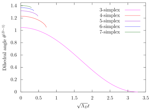
Figure 4: Plots of the dihedral angles of the simplicial polytope models for $3\leq D\leq 7$.

Time-development of the dihedral angle $\theta$ can be obtained by integrating (3.8) numerically for the initial condition (3.10). We give plots of the dihedral angles of simplicial polytope models for $D=3,4,\cdots,7$ and $0\leq t\leq\tau_{\mathrm{p}}/2$ in Figure 4.

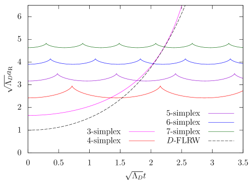
Figure 5: Plots of the scale factors of the simplicial polytope models for $3\leq D\leq 7$. The broken curve corresponds to the $D$-dimensional FLRW universe.

To compare the polytopal universe with the continuum, we must introduce a Regge calculus analog of the scale factor. There are, however, ambiguities in defining a radius of a regular polytope. Here we simply introduce it as the radius of the circumsphere of the regular polytope

$$a_{\mathrm{R}}(t) =\hat{R}_{D}l(t).$$ (3.20)

Inserting the solutions of (3.8) into (3.20), we obtain the time-developments of the scale factors of polytopal universes. Figure 5 shows the behaviors of the simplicial universes. The broken curve corresponds to the $D$-dimensional FLRW solution. The 3-simplicial model expands faster than the continuum one and diverges at $t=\tau_{\mathrm{p}}/2$. For $D\geq 4$, after arriving at the maximum scale $a(\tau_{\mathrm{p}}/2)$ the universe begins to contract to the initial minimum size $a(0)=a(\tau_{\mathrm{p}})$. Then the universe repeats expanding and contracting with a period $\tau_{\mathrm{p}}$. One easily sees that the $D$-simplices are too crude to approximate the continuum solution. The larger the space-time dimensions, the bigger difference we have. The situation is somewhat improved by considering $D$-orthoplices or $D$-cubes in this order. For fixed space-time dimensions the deviation from the continuum FLRW universe become smaller as the number of vertices increases.

In closing this section we comment on the case of $D$-polytopal universe without cosmological constant. In this case the Hamiltonian constraint (3.2) yields $\theta^{(D-1)}=\dfrac{2\pi}{p_{D}}$. We obtain from (3.4)

$$\dot{l}^{2}=-\frac{\cos^{2}\frac{\vartheta_{D-1}}{2}-\cos^{2}\frac{\pi}{p_{D}}}{\hat{R}_{D-1}^{2}\cos^{2}\frac{\vartheta_{D-1}}{2}-\hat{R}_{D-2}^{2}\cos^{2}\frac{\pi}{p_{D}}}=-\frac{1}{\hat{R}_{D}^{2}}.$$ (3.21)

There is no convex regular polytope satisfying this. The Hamiltonian constraint, however, admits infinite honeycomb lattices in flat Euclidean space. For any space-filling honeycomb the circumradius $\hat{R}_{D}$ diverges and the dihedral angle is given by $\vartheta_{D}=\pi$, which immediately yields

$$\cos\frac{\vartheta_{D-1}}{2}=\cos\frac{\pi}{p_{D}}.$$ (3.22)

See (A.14). In Table 3 we summarize space-filling honeycomb lattices in arbitrary dimensions. It is straightforward to verify (3.22). We thus obtain static solutions $l=\mathrm{const}$. They correspond to the Minkowski space-time. In addition, in the case of $\dot{l}^{2}>0$, Schläfli symbol satisfying this inequality stands for a regular lattice of open Cauchy surface of constant negative curvature. These results are consistent with solutions of the Friedmann equations (2.3). See Table 1.

Dimensions $D$	Name	Extended Schläfli symbol	$[D,\kappa_{D},\lambda_{D},\mu_{D},\zeta_{D}]$
2	Apeirogon	$\left\{2,\infty,2\right\}$	$[2,\infty,3,3,3]$
	Triangular tiling	$\left\{2,3,6,2\right\}$	$[3,3,6,3,3]$
3	Square tiling	$\left\{2,4,4,2\right\}$	$[3,4,4,3,3]$
	Hexagonal tiling	$\left\{2,6,3,2\right\}$	$[3,6,3,3,3]$
4	Cubic honeycomb	$\left\{2,4,3,4,2\right\}$	$[4,4,3,4,3]$
	8-cell honeycomb	$\left\{2,4,3,3,4,2\right\}$	$[5,4,3,3,4]$
5	16-cell honeycomb	$\left\{2,3,3,4,3,2\right\}$	$[5,3,3,4,3]$
	24-cell honeycomb	$\left\{2,3,4,3,3,2\right\}$	$[5,3,4,3,3]$
$n+1\geq 6$	$n$-cubic honeycomb $\delta_{n+1}$	$\left\{2,4,3^{n-2},4,2\right\}$	$[n+1,4,3,3,4]$

Table 3: Space-filling lattices in Euclidean $\left(D-1\right)$-space. The lattices for $D\geq 3$ are corresponding to Minkowski space-time. The $n$-cubic honeycomb is named by Coxeter as $\delta_{n+1}$ [17], which has the extended Schläfli symbol $\left\{2,4,3^{n-2},4,2\right\}$. The only misfit is $\delta_{2}=\left\{2,\infty,2\right\}$.

4 Fractional Schläfli symbol and pseudo-regular
$D$-polytopal universes

So far we have investigated evolution of regular polytopes as a discretized FLRW universe. To go beyond the approximation by regular polytopes, we must introduce polytopes with more cells. One way to implement this is to employ geodesic domes [10]. Hypercube is the only type of regular polytope having subdivisions of facets in arbitrary dimensions by the same type of polytopes with the parent facets. In this section we consider hypercube-based geodesic domes as Cauchy surfaces of the universe.

Figure 6: Subdivision of a 3-cube as a cell of a 4-cube for (a) $\nu=2$, (b) $\nu=3$, and (c) $\nu=4$. In four dimensions the peaks are the edges. Solid lines are the three-way connectors and broken lines the four-way connectors.

A hypercube in $D$ dimensions has $(D-1)$-cubes as its facets. To define a geodesic dome for the hypercube we first divide each facet into $\nu^{D-1}$ pieces of $(D-1)$-cubes of edge length $l/\nu$ as depicted in Figure 6, where $\nu$ is the level of the division, called frequency. We then radially project the tessellated hypercube on the circumsphere of the original hypercube. This results in a tessellation of the circumsphere. The geodesic dome $\Gamma_{\nu}$ can be obtained by replacing each circular arc of the tessellated circumsphere with a line segment jointing its end points. In general each facet of $\Gamma_{\nu}$ thus constructed is not a flat $(D-1)$-space. We can always decompose these facets into flat $(D-1)$-polytopes by adding extra edges. The deviations from the flat $(D-1)$-spaces, however, become negligible as $\nu$ increases. We can effectively regard the facets of $\Gamma_{\nu}$ as flat $(D-1)$-cubes and see any polytopal data of the geodesic dome such as the numbers of facets, ridges, etc. from the tessellated $D$-cube.

We can apply Regge calculus to $\Gamma_{\nu}$ as the polyhedral model in Ref. [10]. In the infinite frequency limit $\nu\to\infty$, geodesic dome reproduces a smooth sphere. So the model universe approaches the FLRW universe in the limit $\nu\rightarrow\infty$. In practice the larger the frequency, the more cumbersome the Regge calculus for geodesic domes becomes. We avoid this complexity by introducing pseudo-regular polytopes as in Refs. [10, 11].

Let us denote the pseudo-regular polytope corresponding to $\Gamma_{\nu}$ by $\tilde{\Gamma}_{\nu}$. We assign it a fractional Schläfli symbol

$$\{2,4,3^{D-3},p(\nu),2\},$$ (4.1)

where $p(\nu)$ is the averaged number of facets sharing a peak of $\Gamma_{\nu}$ and the other $D$ integers are the Schläfli symbol of the facets of $\Gamma_{\nu}$. There are two types of peaks of $\Gamma_{\nu}$ as illustrated in Figure 6 for a cell of 4-cube. One is shared by three facets. These come from the peaks of the original $D$-cube. The other connects four facets. They are generated in subdividing the facets of the original $D$-cube. We refer to the former type as “three-way connector” and the later “four-way connector”. Counting the numbers of each type of connectors and averaging the number of facets around a peak in $\Gamma_{\nu}$, we find

$$p(\nu)=\frac{12\nu^{2}}{3\nu^{2}+1}.$$ (4.2)

See Appendix C for details. The result is independent of $D$. Furthermore, the fractional Schläfli symbol approaches the one of $(D-1)$-cubic honeycomb in the limit $\nu\rightarrow\infty$.

The basic approach of pseudo-regular polytope is to regard $\tilde{\Gamma}_{\nu}$ as a regular polytope of edge length $l$ with the fractional Schläfli symbol (4.1) and to assume that the model universe is described by the Regge equations (3.2) and (3.3). The symbol (4.1) corresponds to the assignment

$$p_{2}=4,\quad\lambda_{D-1}=3,\quad p_{D}=p(\nu).$$ (4.3)

In particular the normalized circumradii (3.18) and the dihedral angle (3.19) coincide with those of the regular $D$-cube. They are independent of the frequency $\nu$. The differential equation for the dihedral angle $\theta(t)$ can be written explicitly as

$$\dot{\theta}(t) =\mp\frac{2}{2\pi-p(\nu)\left(\theta(t)-\sin\theta(t)\right)}\sqrt{\frac{p(\nu)\Lambda_{D}\left(2\pi-p(\nu)\theta(t)\right)\sin 2\theta(t)}{1-\left(D-2\right)\cos\theta(t)}}\sin\frac{\theta(t)}{2}.$$ (4.4)

Note that the initial dihedral angle is $\theta(0)=\theta_{0}=\vartheta_{D-1}=\pi/2$. Both $\theta_{0}$ and $\theta_{\mathrm{c}}=\arccos\dfrac{1}{D-2}$ do not depend on $\nu$.

The scale factor $a_{\mathrm{R}}$ for the pseudo-regular $D$-polytopal universe can be defined similarly as the regular polytopal models as

$$a_{\rm R}\left(t\right) =\hat{R}_{D}(\nu)l(t),$$ (4.5)

where the edge length $l(t)$ for $\tilde{\Gamma}_{\nu}$ can be found from (3.5) as

$$l(t)=\frac{2}{\sqrt{\Lambda_{D}}}\sqrt{\left(\frac{2\pi}{p(\nu)}-\theta(t)\right)\cot\frac{\theta(t)}{2}}.$$ (4.6)

The normalized circumradius $\hat{R}_{D}(\nu)$ also depends on $p_{D}=p(\nu)$ and can be obtained from (3.16) as

$$\hat{R}_{D}(\nu)=\frac{1}{2}\sqrt{D-2-\sec\frac{2\pi}{p(\nu)}}.$$ (4.7)

For $\nu=1$ this coincides with the circumradius of a regular $D$-cube of unit edge length. It grows with the frequency $\nu$ and diverges linearly for $\nu\rightarrow\infty$. In fact Eq. (4.7) can be approximated for large frequency by

$$\hat{R}_{D}(\nu)\approx\sqrt{\frac{3}{2\pi}}\nu.$$ (4.8)

On the other hand the edge length (4.6) decreases roughly inversely with $\nu$ and approaches zero as $\nu\rightarrow\infty$. This can be seen explicitly for the initial edge length

$$l(0)=\sqrt{\frac{2\pi}{3\Lambda_{D}}}\frac{1}{\nu}.$$ (4.9)

The scale factor (4.5), however, remains finite for $\nu\rightarrow\infty$. Noting that $\hat{R}_{D-k}$ ($k=1,2,3$) are independent of $\nu$ as given by (3.18), it is straightforward to verify that the Regge equations (3.2) and (3.3) for $\tilde{\Gamma}_{\nu}$ reduce to the Friedmann equations (2.3) in the limit $\nu\rightarrow\infty$.

To see the dependences on $\nu$ we give plots of the dihedral angles in Figure 7 and those of the scale factors in Figure 8 for $D=5$, $\nu\leq 5$, and $0\leq t\leq\tau_{\mathrm{p}}(\nu)/2$, where $\tau_{\mathrm{p}}(\nu)$ is the period of the oscillation of $\tilde{\Gamma}_{\nu}$. One might think that $D$-cube-based pseudo-regular polytopes are too crude to approximate $D$-spheres. As can be seen from Figure 8, the scale factor approaches rapidly the continuum one as $\nu$ increases. As mentioned above, the geodesic dome $\Gamma_{\nu}$ becomes impractical to carry out Regge calculus for large $\nu$. The advantage of the approach of pseudo-regular polytopes is its applicability to arbitrarily large frequency without effort. The scale factor for $\nu=100$ is shown in Figure 9. Coincidence with the continuum theory is excellent for $\sqrt{\Lambda_{5}}t\sim 4$. The edge length becomes comparable with $1/\sqrt{\Lambda_{5}}$ at around $\sqrt{\Lambda_{5}}t\sim 4$, onset of the deviation from the continuum solution.

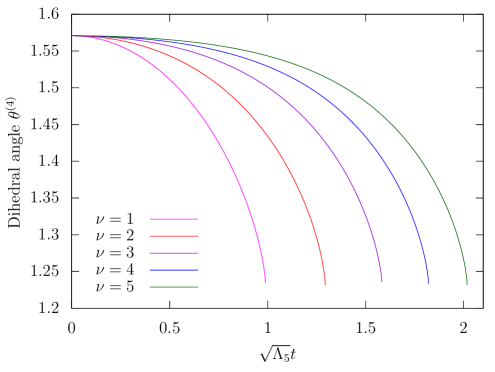
Figure 7: Plots of the dihedral angles of the pseudo-regular 5-polytopal universes for $\nu\leq 5$.

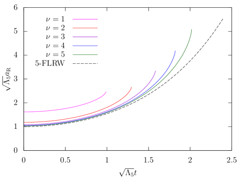
Figure 8: Plots of the scale factors of the pseudo-regular 5-polytopal universes for $\nu\leq 5$. The broken curve corresponds to the five-dimensional FLRW universe.

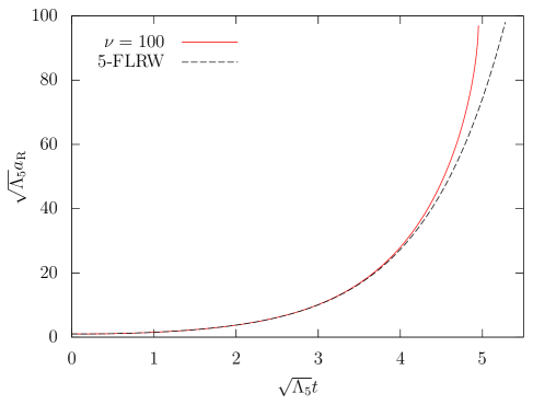
Figure 9: Plot of the scale factor of the pseudo-regular 5-polytopal universe for $\nu=100$. The broken curve stands for the exact solution of the continuum theory.

5 Summary and discussions

Following the CW formalism, we have carried out Regge calculus for closed FLRW universe with a positive cosmological constant in arbitrary dimensions. The geometrical characterization of regular polytopes by the Schläfli symbol has turned out to be very efficient in describing systematically the discrete FLRW universe in spite of there being only three types of regular polytopes in dimensions more than four. We have given the Regge action in closed form in the continuum time limit. It possesses a reparameterization invariance of time variable to ensure coordinate independence of the formalism. The Regge equations are the Hamiltonian constraint and the evolution equation as the continuum theory, describing the time development of the discrete FLRW universe. They coincide with the previous results in three and four dimensions [10, 11]. In particular under the gauge choice (3.1) the circumsphere of the regular polytope repeats periodically expansion and shrinking in any dimensions larger than four as the four dimensional case. The Regge equations have more or less the same structures in dimensions greater than three. It is only in three dimensions where the edge length diverges in finite time.

As we have shown in Sect. 3 the approximation by regular polytopes is not so accurate even for $\sqrt{\Lambda_{D}}t\ll 1$. The situation gets worse as the dimensions increase. This is contrasted with the cases of dodecahedron in three dimensions and 120-cell in four dimensions, which describe the continuum FLRW universe rather well until $t$ becomes comparable with $1/\sqrt{\Lambda_{D}}$. The difference basically comes from that of the number of vertices in a polytope. A 120-cell has six hundred vertices, whereas a 4-cube does only sixteen. In five or more dimensions there are no such special polytopes. One must refine the tessellation of the Cauchy surface by nonregular polytopes with smaller cells to have better approximations. Though this can be done by extending the geodesic domes in three dimensions, we have analyzed pseudo-regular polytopes with the expectation that the Regge equations for the pseudo-regular polytopes approximate well the Regge calculus of the corresponding geodesic domes. We stress that the pseudo-regular polytope is a substitute of the corresponding geodesic domes characterized by the frequency $\nu$, not the continuum hypersphere. The Regge equations (3.2) and (3.3) therefore should be considered as an effective description of the Regge equations for the geodesic dome, not of the continuum Freedman equations. The approach of pseudo-regular polytopes can be applied to an arbitrary $\nu$. In particular we can infer the validity of Regge calculus for geodesic domes. Because of this, the pseudo-regular polytope universe begins to deviate from the continuum solution when the edge length becomes larger than $1/\sqrt{\Lambda_{D}}$.

In this paper we have considered vacuum universes without matters. Incorporating gravitating matter sources is worth investigation. In General Relativity, Friedmann equations have a solution for a negative cosmological constant. It describes hyperbolic Cauchy surfaces expanding or contracting with time. Applying the method of pseudo-regular polytope to such non-compact universe be interesting. We will address these issues elsewhere.

Appendix A Circumradii and dihedral angles of regular polytopes

In this appendix we give closed expressions for circumradius and dihedral angle of an arbitrary regular polytope $\Pi_{n}=\left\{p_{1},\cdots,p_{n},p_{0}\right\}$ in $n$ dimensions [17, 18]. By definition $\Pi_{n}$ has regular $(n-1)$-polytopes $\Pi_{n-1}=\{p_{1},\cdots,p_{n-1},p_{0}\}$ as its $N^{(n)}_{n-1}$ cells. Each cell of $\Pi_{n}$ also has $N^{(n-1)}_{n-2}$ cells. They are regular $(n-2)$-polytopes $\Pi_{n-2}=\{p_{1},\cdots,p_{n-2},p_{0}\}$. Similar decomposition of a daughter cell of a parent cell can be continued until we arrive at the vertices of the original $n$-polytope. They are zero-dimensional cells $\Pi_{0}=\{p_{0}\}$. Incidentally $\Pi_{1}=\{p_{1},p_{0}\}$ corresponds to edges.

We now choose a set of cells $\Pi_{0}$, $\Pi_{1}$, $\cdots$, $\Pi_{n-1}$ satisfying $\Pi_{0}\subset\Pi_{1}\subset\cdots\subset\Pi_{n-1}\subset\Pi_{n}$ and denote the centers of circumspheres of the $\Pi_{k}$ by $\mathrm{O}_{k}$ ($k=0,1,\cdots,n$). See Figure 10(a). Then $R_{n}=\overline{\mathrm{O}_{n}\mathrm{O}_{0}}$ is the circumradius of $\Pi_{n}$. It is given by

$$R_{n}=l\hat{R}_{n}\quad\hbox{with}\quad\hat{R}_{n}=\frac{1}{2}\csc\phi,$$ (A.1)

where $l$ is the edge length of the original regular polytope $\Pi_{n}$ and the angle $\phi$ is defined by

$$\phi=\angle\mathrm{O}_{0}\mathrm{O}_{n}\mathrm{O}_{1}.$$ (A.2)

Note that the line segments connecting $\mathrm{O}_{k}$ and $\mathrm{O}_{k+1}$ ($k=0,1,\cdots,n-1$) are orthogonal to one another.

Figure 10: (a) Centers of circumspheres of the $\Pi_{k}~{}\left(k=0,1,\cdots,n\right)$ in the case of $\Pi_{3}=\left\{2,3,3,2\right\}$, where $n$ is the dimension of original regular polytope $\Pi_{n}$. Obviously $\mathrm{O}_{1}$ is just the midpoint of $\Pi_{1}$ and $\mathrm{O}_{0}=\Pi_{0}$. (b) $\mathrm{O}^{\prime}_{0},\mathrm{O}^{\prime}_{1},\cdots,\mathrm{O}^{\prime}_{n-1}$ are the centers in the vertex figure $\Pi^{\prime}_{n-1}$ and (c) $R_{n}$ and $R^{\prime}_{n-1}$ are the circumradii of $\Pi_{n}$ and $\Pi^{\prime}_{n-1}$, respectively.

We next consider the section obtained by cutting out $\Pi_{n}$ by the hyperplane through the centers of edges meeting at $\mathrm{O}_{0}$. It is a regular $(n-1)$-polytope $\Pi^{\prime}_{n-1}=\{p_{1},p_{3},\cdots,p_{n},p_{0}\}$, called vertex figure, of an edge length $l^{\prime}=l\cos\dfrac{\pi}{p_{2}}$. We can pick up a sequence of centers $\mathrm{O}_{0}^{\prime}(=\mathrm{O}_{1})$, $\mathrm{O}_{1}^{\prime}$, $\mathrm{O}_{2}^{\prime}$, $\cdots$, $\mathrm{O}_{n-1}^{\prime}$ in $\Pi_{n-1}^{\prime}$ as we have done for $\Pi_{n}$. See Figure 10(b). The circumradius of $\Pi^{\prime}_{n-1}$ is given by $R_{n-1}^{\prime}=\dfrac{l^{\prime}}{2}\csc\phi^{\prime}=\dfrac{l}{2}\csc\phi^{\prime}\cos\dfrac{\pi}{p_{2}}$ with $\phi^{\prime}=\angle\mathrm{O}_{0}^{\prime}\mathrm{O}_{n-1}^{\prime}\mathrm{O}_{1}^{\prime}$. We can also write it as $R_{n-1}^{\prime}=\dfrac{l}{2}\cos\phi$ since $\triangle\mathrm{O}_{0}\mathrm{O}_{1}\mathrm{O}_{n-1}^{\prime}$ is similar to the right triangle $\triangle\mathrm{O}_{0}\mathrm{O}_{1}\mathrm{O}_{n}$ as depicted in Figure 10(c). These lead to a constraint between the angles $\phi$ of $\Pi_{n}=\{p_{1},p_{2},\cdots,p_{n},p_{0}\}$ and $\phi^{\prime}$ of $\Pi^{\prime}_{n-1}=\{p_{1},p_{3},\cdots,p_{n},p_{0}\}$ as

$$\cos\phi=\csc\phi^{\prime}\cos\frac{\pi}{p_{2}}\quad\hbox{or}\quad\sin^{2}\phi=1-\frac{\cos^{2}\frac{\pi}{p_{2}}}{\sin^{2}\phi^{\prime}}.$$ (A.3)

We thus obtain $\sin^{2}\phi$ in terms of a continued fraction as

$$\sin^{2}\phi=1-\frac{\cos^{2}\frac{\pi}{p_{2}}}{1-}\frac{\cos^{2}\frac{\pi}{p_{3}}}{1-}\cdots\frac{\cos^{2}\frac{\pi}{p_{n-2}}}{1-}\frac{\cos^{2}\frac{\pi}{p_{n-1}}}{\sin^{2}\frac{\pi}{p_{n}}}.$$ (A.4)

More tractable expressions for the normalized circumradius $\hat{R}_{n}$ can be found by applying the substitution rules[11]

$$\begin{cases}\sin^{2}\frac{\pi}{p_{k-1}}&\to~{}\sin^{2}\frac{\pi}{p_{k-1}}\sin^{2}\frac{\pi}{p_{k+1}}\\ \cos^{2}\frac{\pi}{p_{k-1}}&\to~{}\cos^{2}\frac{\pi}{p_{k-1}}\sin^{2}\frac{\pi}{p_{k+1}}\\ \sin^{2}\frac{\pi}{p_{k-2}}&\to~{}\sin^{2}\frac{\pi}{p_{k-2}}\left(1-\csc^{2}\frac{\pi}{p_{k}}\cos^{2}\frac{\pi}{p_{k+1}}\right)\\ \cos^{2}\frac{\pi}{p_{k-2}}&\to~{}\cos^{2}\frac{\pi}{p_{k-2}}\left(1-\csc^{2}\frac{\pi}{p_{k}}\cos^{2}\frac{\pi}{p_{k+1}}\right)\end{cases}$$ (A.5)

to $\hat{R}_{k}$ with the initial condition

$$\hat{R}_{1}=\frac{1}{2}\sqrt{\frac{\sin^{2}\frac{\pi}{p_{1}}}{\sin^{2}\frac{\pi}{p_{0}}}}.$$ (A.6)

For reader’s reference we give the next four of the circumradii

$$\hat{R}_{2} =\frac{1}{2}\sqrt{\frac{\sin^{2}\frac{\pi}{p_{1}}}{\sin^{2}\frac{\pi}{p_{0}}\sin^{2}\frac{\pi}{p_{2}}}},$$ (A.7)

$$\hat{R}_{3} =\frac{1}{2}\sqrt{\frac{\sin^{2}\frac{\pi}{p_{1}}\sin^{2}\frac{\pi}{p_{3}}}{\sin^{2}\frac{\pi}{p_{0}}\left(\sin^{2}\frac{\pi}{p_{2}}-\cos^{2}\frac{\pi}{p_{3}}\right)}},$$ (A.8)

$$\hat{R}_{4} =\frac{1}{2}\sqrt{\frac{\sin^{2}\frac{\pi}{p_{1}}\left(\sin^{2}\frac{\pi}{p_{3}}-\cos^{2}\frac{\pi}{p_{4}}\right)}{\sin^{2}\frac{\pi}{p_{0}}\left(\sin^{2}\frac{\pi}{p_{2}}\sin^{2}\frac{\pi}{p_{4}}-\cos^{2}\frac{\pi}{p_{3}}\right)}},$$ (A.9)

$$\hat{R}_{5} =\frac{1}{2}\sqrt{\frac{\sin^{2}\frac{\pi}{p_{1}}\left(\sin^{2}\frac{\pi}{p_{3}}\sin^{2}\frac{\pi}{p_{5}}-\cos^{2}\frac{\pi}{p_{4}}\right)}{\sin^{2}\frac{\pi}{p_{0}}\left(\sin^{2}\frac{\pi}{p_{2}}\left(\sin^{2}\frac{\pi}{p_{4}}-\cos^{2}\frac{\pi}{p_{5}}\right)-\cos^{2}\frac{\pi}{p_{3}}\sin^{2}\frac{\pi}{p_{5}}\right)}},$$ (A.10)

where $p_{0}=p_{1}=2$. One can easily see that (A.4) reproduces the same results.

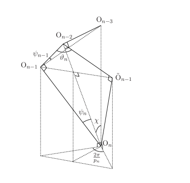
Figure 11: $\mathrm{O}_{n}$ is the circumcenter of $\Pi_{n}$. $\mathrm{O_{n-1}}$ and $\mathrm{\tilde{O}}_{n-1}$ are the centers of two facets sharing a ridge $\Pi_{n-2}$ centered at $\mathrm{O}_{n-2}$, and $\mathrm{O}_{n-3}$ is located at the center of a peak $\Pi_{n-3}$ included in the $\Pi_{n-2}$.

Returning to the set of points $\mathrm{O}_{0}$, $\mathrm{O}_{1}$, $\cdots$, $\mathrm{O}_{n}$ in $\Pi_{n}$, we define angles

$$\psi_{n}=\angle\mathrm{O}_{n-2}\mathrm{O}_{n}\mathrm{O}_{n-1},\quad\psi_{n-1}=\angle\mathrm{O}_{n-3}\mathrm{O}_{n-1}\mathrm{O}_{n-2},\quad\chi=\angle\mathrm{O}_{n-3}\mathrm{O}_{n}\mathrm{O}_{n-2}.$$ (A.11)

See Figure 11. The dihedral angle $\vartheta_{n}$ between the two facets of $\Pi_{n}$ connected at the ridge $\Pi_{n-2}$ is related to $\psi_{n}$ by

$$\vartheta_{n}=\pi-2\psi_{n}.$$ (A.12)

To see this consider a pair of adjacent facets of $\Pi_{n}$, one is the $\Pi_{n-1}$ centered at $\mathrm{O}_{n-1}$ and the other centered at $\tilde{\mathrm{O}}_{n-1}$. The four points $\mathrm{O}_{n}$, $\mathrm{O}_{n-1}$, $\mathrm{O}_{n-2}$, $\tilde{\mathrm{O}}_{n-1}$ with $\angle\mathrm{O}_{n-2}\mathrm{O}_{n-1}\mathrm{O}_{n}=\angle\mathrm{O}_{n-2}\tilde{\mathrm{O}}_{n-1}\mathrm{O}_{n}=\dfrac{\pi}{2}$ lie on a two dimensional plane, from which (A.12) immediately follows.

There are $p_{n}$ such planes around the axis $\mathrm{O}_{n-3}\mathrm{O}_{n}$. This implies that the projections of $\mathrm{O}_{n-1}\mathrm{O}_{n}$ and $\tilde{\mathrm{O}}_{n-1}\mathrm{O}_{n}$ onto the plane perpendicular to $\mathrm{O}_{n-3}\mathrm{O}_{n}$ in the three dimensional space containing $\mathrm{O}_{n-3}$, $\mathrm{O}_{n-2}$, $\mathrm{O}_{n-1}$, and $\mathrm{O}_{n}$ make an angle $\dfrac{2\pi}{p_{n}}$. It can be seen that the three angles (A.11) satisfy $\tan\chi=\sin\psi_{n}\tan\psi_{n-1}$ and $\tan\psi_{n}=\sin\chi\tan\dfrac{\pi}{p_{n}}$, from which we obtain

$$\sin\psi_{n-1}\cos\psi_{n}=\cos\frac{\pi}{p_{n}}.$$ (A.13)

This enables us to express $p_{n}$ in terms of the dihedral angles as

$$p_{n}=\frac{\pi}{\arccos\left(\cos\frac{\vartheta_{n-1}}{2}\sin\frac{\vartheta_{n}}{2}\right)}.$$ (A.14)

Eq. (A.13) can be written as

$$\sin^{2}\psi_{n}=1-\frac{\cos^{2}\frac{\pi}{p_{n}}}{\sin^{2}\psi_{n-1}}.$$ (A.15)

One easily recognize similarity to (A.3). We thus arrive at an expression for the dihedral angle $\vartheta_{n}$ in terms of a continued fraction as

$$\vartheta_{n}=2\arcsin\sqrt{\frac{\cos^{2}\frac{\pi}{p_{n}}}{1-}\frac{\cos^{2}\frac{\pi}{p_{n-1}}}{1-}\cdots\frac{\cos^{2}\frac{\pi}{p_{4}}}{1-}\frac{\cos^{2}\frac{\pi}{p_{3}}}{\sin^{2}\frac{\pi}{p_{2}}}}.$$ (A.16)

Eq. (A.12) for $n=2$ gives

$$\vartheta_{2}=\pi-\frac{2\pi}{p_{2}}=2\arcsin\left(\cos\frac{\pi}{p_{2}}\right),$$ (A.17)

which is the interior angle of a regular polygon $\{p_{1},p_{2},p_{0}\}$. The next three dihedral angles are explicitly given by

$$\vartheta_{3} =2\arcsin\frac{\cos\frac{\pi}{p_{3}}}{\sin\frac{\pi}{p_{2}}},$$ (A.18)

$$\vartheta_{4} =2\arcsin\frac{\sin\frac{\pi}{p_{2}}\cos\frac{\pi}{p_{4}}}{\sqrt{\sin^{2}\frac{\pi}{p_{2}}-\cos^{2}\frac{\pi}{p_{3}}}},$$ (A.19)

$$\vartheta_{5} =2\arcsin\left(\sqrt{\frac{\sin^{2}\frac{\pi}{p_{2}}-\cos^{2}\frac{\pi}{p_{3}}}{\sin^{2}\frac{\pi}{p_{2}}\sin^{2}\frac{\pi}{p_{4}}-\cos^{2}\frac{\pi}{p_{3}}}}\cos\frac{\pi}{p_{5}}\right).$$ (A.20)

Moreover Eq. (A.14) with (A.17) gives a natural extension of $\vartheta_{n}$ for a 1-polytope as

$$\vartheta_{1}=0.$$ (A.21)

It is possible to write the circumradius in terms of the dihedral angles without using continued fraction. To do this let us denote the distance between $\mathrm{O}_{k-1}$ and $\mathrm{O}_{k}$ by $d_{k}$ ($k=1,\cdots,n$), then $d_{k+1}=d_{k}\tan\dfrac{\vartheta_{k+1}}{2}$ with $d_{1}=\dfrac{l}{2}$. The square of normalized circumradius can be expressed as

$$\hat{R}_{n}^{2}=\frac{1}{l^{2}}\sum_{j=1}^{n}d_{j}^{2}=\frac{1}{4}\left(1+\sum_{j=2}^{n}\prod_{k=2}^{j}\tan^{2}\frac{\vartheta_{k}}{2}\right)\qquad(n\geq 2).$$ (A.22)

It is easy to show the following recurrence relations

$$\hat{R}_{n}^{2}-\hat{R}_{n-1}^{2}=(\hat{R}_{n-1}^{2}-\hat{R}_{n-2}^{2})\tan^{2}\frac{\vartheta_{n}}{2},$$ (A.23)

$$\frac{\hat{R}_{n-2}^{2}}{\hat{R}^{2}_{n-1}}\sin^{2}\frac{\vartheta_{n}}{2}=\frac{\cos^{2}\frac{\pi}{p_{n}}}{1-\dfrac{\hat{R}_{n-3}^{2}}{\hat{R}^{2}_{n-2}}\sin^{2}\dfrac{\vartheta_{n-1}}{2}}.$$ (A.24)

The second of these leads to

$$\frac{\hat{R}_{n-2}^{2}}{\hat{R}^{2}_{n-1}}\sin^{2}\frac{\vartheta_{n}}{2}=\frac{\cos^{2}\frac{\pi}{p_{n}}}{1-}\frac{\cos^{2}\frac{\pi}{p_{n-1}}}{1-}\cdots\frac{\cos^{2}\frac{\pi}{p_{4}}}{\sin^{2}\frac{\pi}{p_{3}}}.$$ (A.25)

Comparing this with (A.16), we see $2\arcsin\left(\dfrac{\hat{R}_{n-2}}{\hat{R}_{n-1}}\sin\frac{\vartheta_{n}}{2}\right)$ coincides with a dihedral angle of a regular $(n-1)$-polytope $\{p_{1},p_{3},\cdots,p_{n},p_{0}\}$. It is a vertex figure of $\Pi_{n}$.

In six or higher dimensions every convex regular polytope and space-filling lattice have Schläfli symbol $p_{5}=\cdots=p_{n-1}=3$ in common as given in Tables 2 and 3. Therefore in these dimensions the circumradius and the dihedral angle of a regular $n$-polytope depend on only five parameters $p_{2}$, $p_{3}$, $p_{4}$, $p_{n}$, and $n$. Inserting $p_{0}=p_{1}=2$ and $p_{5}=\cdots=p_{n-1}=3$ into (A.4) and (A.16), we obtain the general forms of the circumradius and the dihedral angle of a unit equilateral polytope for $n\geq 5$ as

$$\hat{R}_{n} =\frac{1}{2}\sqrt{\frac{\left[1-\left(D-4\right)\cos\frac{2\pi}{p_{n}}\right]\sin^{2}\frac{\pi}{p_{3}}-2\left[1-\left(D-5\right)\cos\frac{2\pi}{p_{n}}\right]\cos^{2}\frac{\pi}{p_{4}}}{\left[1-\left(D-4\right)\cos\frac{2\pi}{p_{n}}\right]\left(\sin^{2}\frac{\pi}{p_{3}}-\cos^{2}\frac{\pi}{p_{2}}\right)-2\left[1-\left(D-5\right)\cos\frac{2\pi}{p_{n}}\right]\sin^{2}\frac{\pi}{p_{2}}\cos^{2}\frac{\pi}{p_{4}}}},$$ (A.26)

$$\vartheta_{n} =2\arcsin\left(\sqrt{2\frac{\sin^{2}\frac{\pi}{p_{2}}\left[1-\left(D-5\right)\cos\frac{2\pi}{p_{4}}\right]-\left(D-4\right)\cos^{2}\frac{\pi}{p_{3}}}{\sin^{2}\frac{\pi}{p_{2}}\left[1-\left(D-4\right)\cos\frac{2\pi}{p_{4}}\right]-\left(D-3\right)\cos^{2}\frac{\pi}{p_{3}}}}\cos\frac{\pi}{p_{n}}\right).$$ (A.27)

Appendix B Dihedral angles of a $(D-1)$-polytopal frustum

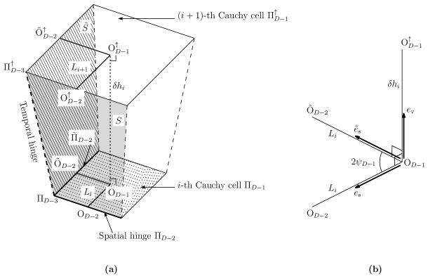
Figure 12: (a) $(D-1)$-polytopal frustum and (b) three unit vectors $e_{\mathrm{s}}$, $\tilde{e}_{\mathrm{s}}$, and $e_{\mathrm{v}}$ parallel to $\mathrm{O}_{D-1}\mathrm{O}_{D-2}$, $\mathrm{O}_{D-1}\tilde{\mathrm{O}}_{D-2}$, and $\mathrm{O}_{D-1}\mathrm{O}^{\uparrow}_{D-1}$, respectively.

In this appendix we give a derivation of the dihedral angles (2.13) and (2.14).

We first consider a temporal hinge. Let us choose an $i$-th $(D-1)$-polytopal frustum with $\Pi_{D-1}^{\uparrow}$ and $\Pi_{D-1}$ as the upper and lower cells as illustrated schematically in Figure 12(a). The hinge is supposed to contain the regular $(D-3)$-polytopes $\Pi_{D-3}$ and $\Pi^{\uparrow}_{D-3}$. Each vertex of $\Pi_{D-3}$ is connected with the corresponding vertex of $\Pi^{\uparrow}_{D-3}$ by a strut. The height of the frustum $\delta h_{i}$ and the distance $L_{i}$ between $\mathrm{O}_{D-1}$ and $\mathrm{O}_{D-2}$ are given by

$$\delta h_{i}=\sqrt{m_{i}^{2}-\hat{R}_{D-1}^{2}\delta l_{i}^{2}},\qquad L_{i}=\sqrt{\hat{R}_{D-1}^{2}-\hat{R}_{D-2}^{2}}~{}l_{i}.$$ (B.1)

As illustrated in Figure 12(a) there are two lateral cells jointed at the temporal hinge, one containing $\Pi_{D-2}$ and the other containing $\tilde{\Pi}_{D-2}$. Let $S$ be the $(D-1)$-dimensional hyperplane containing $\Pi_{D-2}$ and $\Pi^{\uparrow}_{D-3}$, then the outgoing unit normal to $S$ can be written as

$$u=\frac{\delta h_{i}e_{\mathrm{s}}-\delta L_{i}e_{\mathrm{v}}}{\sqrt{\delta h_{i}^{2}+\delta L_{i}^{2}}}$$ (B.2)

with $\delta L_{i}=\sqrt{\hat{R}_{D-1}^{2}-\hat{R}_{D-2}^{2}}\delta l_{i}$, where $e_{\mathrm{s}}$ and $e_{\mathrm{v}}$ are, as depicted in Figure 12(b), the unit vectors parallel to $\mathrm{O}_{D-1}\mathrm{O}_{D-2}$ and $\mathrm{O}_{D-1}\mathrm{O}_{D-1}^{\uparrow}$, respectively. Likewise, we set up the hyperplane $\tilde{S}$ as the section containing $\tilde{\Pi}_{D-2}$ and $\Pi^{\uparrow}_{D-3}$. Then the outgoing unit normal to $\tilde{S}$ takes the form

$$\tilde{u}=\frac{\delta h_{i}\tilde{e}_{\mathrm{s}}-\delta L_{i}e_{\mathrm{v}}}{\sqrt{\delta h_{i}^{2}+\delta L_{i}^{2}}},$$ (B.3)

where $\tilde{e}_{\mathrm{s}}$ is the unit vector parallel to $\mathrm{O}_{D-1}\tilde{\mathrm{O}}_{D-2}$. Since $e_{\mathrm{s}}\cdot\tilde{e}_{\mathrm{s}}=\cos 2\psi_{D-1}=-\cos\vartheta_{D-1}$, we can find the dihedral angle $\theta^{(D-1)}_{i}$ from

$$\cos\theta^{(D-1)}_{i}=-u\cdot\tilde{u}=\frac{\delta h_{i}^{2}\cos\vartheta_{D-1}-\delta L_{i}^{2}}{\delta h_{i}^{2}+\delta L_{i}^{2}}.$$ (B.4)

Eq. (2.13) follows from this.

We next turn to the dihedral angle between the two cells meeting at the spatial hinge $\Pi_{D-2}$, one is the $\Pi_{D-1}$ and the other is the hyperplane $S$ defined above. The ingoing unit normal to $\Pi_{D-1}$ is simply $e_{\mathrm{v}}$. The dihedral angle $\phi^{(D-1)\uparrow}$ is then determined by

$$\cos\phi^{(D-1)\uparrow}=u\cdot e_{\mathrm{v}}=-\frac{\delta L_{i}}{\sqrt{\delta h_{i}^{2}+\delta L_{i}^{2}}},$$ (B.5)

from which (2.14) follows.

Appendix C Derivation of $p(\nu)$

In this appendix we give a brief account of Eq. (4.2). As in Sect. 2 we denote the number of $j$-cubes in a $D$-cube by $N^{(D)}_{j}$. It is given by

$$N^{(D)}_{j}=2^{D-j}{D\choose j}\qquad(0\leq j\leq D).$$ (C.1)

Each $j$-dimensional face ($0\leq j\leq D-1$) of the parent $D$-cube is subdivided into $\nu^{j}$ $j$-cubes in the geodesic dome $\Gamma_{\nu}$. Noting that every three-way connector in $\Gamma_{\nu}$ comes from one of the peaks of the original $D$-cube, we find the number of three-way connectors ${\cal N}_{3}$ in $\Gamma_{\nu}$ as

$${\cal N}_{3}=8{D\choose 3}\nu^{D-3}.$$ (C.2)

Since $\Gamma_{\nu}$ has $N^{(D)}_{D-1}\nu^{D-1}$ facets and each of them contains $N^{(D-1)}_{D-3}$ peaks of $\Gamma_{\nu}$, ${\cal N}_{3}$ and the number of four-way connectors ${\cal N}_{4}$ in $\Gamma_{\nu}$ are constrained by

$$3{\cal N}_{3}+4{\cal N}_{4}=N^{(D-1)}_{D-3}N^{(D)}_{D-1}\nu^{D-1}.$$ (C.3)

This together with (C.1) and (C.2) leads to

$${\cal N}_{4}=6{D\choose 3}(\nu^{2}-1)\nu^{D-3}.$$ (C.4)

The averaged number of facets sharing a peak of $\Gamma_{\nu}$ is given by

$$p(\nu)=\frac{3{\cal N}_{3}+4{\cal N}_{4}}{{\cal N}_{3}+{\cal N}_{4}}.$$ (C.5)

It yields Eq. (4.2).