Beta families arising from a $v_{2}^{9}$ self map on $S/(3,v_{1}^{8})$

Abstract.

We show that $v_{2}^{9}$ is a permanent cycle in the 3-primary Adams-Novikov spectral sequence computing $\pi_{*}(S/(3,v_{1}^{8}))$, and use this to conclude that the families $\beta_{9t+3/i}$ for $i=1,2$, $\beta_{9t+6/i}$ for $i=1,2,3$, $\beta_{9t+9/i}$ for $i=1,\dots,8$, $\alpha_{1}\beta_{9t+3/3}$, and $\alpha_{1}\beta_{9t+7}$ are permanent cycles in the 3-primary Adams-Novikov spectral sequence for the sphere for all $t\geq 0$. We use a computer program by Wang to determine the additive and partial multiplicative structure of the Adams-Novikov $E_{2}$ page for the sphere in relevant degrees. The $i=1$ cases recover previously known results of Behrens-Pemmaraju [BP04] and the second author [Shi10]. The results about $\beta_{9t+3/3}$, $\beta_{9t+6/3}$ and $\beta_{9t+9/8}$ were previously claimed by the second author [Shi06]; the computer calculations allow us to give a more direct proof. As an application, we determine the image of the Hurewicz map $\pi_{*}S\to\pi_{*}\mathit{tmf}$ at $p=3$.

1. Introduction

Miller, Ravenel, and Wilson showed that the 2-line of the Adams-Novikov $E_{2}$ page for the sphere is generated by classes $\beta_{i/j,k}$ for $i,j,k$ satisfying certain conditions [MRW77, Theorem 2.6]. At the prime 3, the $\beta$ elements with $i\leq 9$ are:

$$\beta_{i}\text{ for $i=1,2,4,5,7,8$};$$

$$\beta_{3/j}\text{ and }\beta_{6/j}\text{ for $j=1,2,3$};$$

$$\beta_{9/j}\text{ for $j=1,\dots,9$};$$

$$\beta_{9/3,2};$$

where we write $\beta_{i/j}:=\beta_{i/j,1}$ and $\beta_{i}:=\beta_{i/1}$. They have order 3 except for $\beta_{9/3,2}$, which satisfies $3\beta_{9/3,2}=\beta_{9/3}$. Of these, the permanent cycles are the following:

(1.1) $$\beta_{1},\ \beta_{2},\ \beta_{3/2},\ \beta_{3},\ \beta_{5},\ \beta_{6/3},\ \beta_{6/2},\ \beta_{6},\ \beta_{7}+c\beta_{9/9}\text{ for some $c\in\{\pm 1\}$},\ \beta_{9/j}\text{ for $1\leq j\leq 8$}.$$

For $i\leq 7$ and $\beta_{7}+c\beta_{9/9}$, these assertions can be read off the exhaustive calculation [Rav86, Table A3.4] of $\pi_{n}S^{\wedge}_{3}$ in stems $n\leq 108$; see also [Oka81] for many of the survival results and [Shi97] for the non-survival results. The element $\beta_{7}+c\beta_{9/9}$ is an Arf invariant class (an odd-primary analogue of the $p=2$ Kervaire invariant classes), discussed in [Rav78, p.439]; the survival of the Arf invariant classes is not known in general at $p=3$. The survival of $\beta_{9/j}$ for $j\leq 8$ is a consequence of Theorem 5.1, which does not depend on prior knowledge about this element, but we do not claim originality for this result.

These results arise from exhaustive calculations in tractable stems, but it is possible to prove results about $\beta$ elements outside the range of feasible computation. One strategy is as follows. Suppose $\beta_{i/j}$ is a permanent cycle. It is $v_{1}$-power-torsion; that is, there exists a type 2 complex $V$ such that $\beta_{i/j}$ factors as $S\overset{f_{1}}{\to}V\overset{f_{2}}{\to}S$ (we omit degree shifts for clarity of notation). If $v_{2}^{t}$ is a $v_{2}$ self map on $V$, then we may construct elements of $\pi_{*}(S)$ as follows:

$$S\overset{f_{1}}{\longrightarrow}V\overset{v_{2}^{t}}{\longrightarrow}V\overset{f_{2}}{\longrightarrow}S,\hskip 20.0ptt\geq 0.$$

For this family to be of interest, one must also show that the elements are nonzero, for example by identifying their Adams-Novikov representatives.

Let $S/3$ denote the mod 3 Moore space, and for $m\geq 1$ let $S/(3,v_{1}^{m})$ denote the cofiber of the $m$-fold iterate of Adams’ $v_{1}$ self map $S/3\overset{v_{1}}{\longrightarrow}S/3$ [Tod71]. Behrens and Pemmaraju [BP04] show there is a $v_{2}^{9}$ self map on $S/(3,v_{1})$ and use this to prove the existence of nonzero homotopy classes represented by $\beta_{9t+s}$ for $s=1,2,5,6,9$ and $t\geq 0$. The second author [Shi10] proves the existence of $\beta_{9t+3}$. By comparison to $L_{2}$-local homotopy [Shi97], he shows that the elements

$$\beta_{9t+4},\ \beta_{9t+7},\ \beta_{9t+8},\ \beta_{9t+3/3},\ \beta_{9t/3,2},\ \beta_{3^{i}s/3^{i}}$$

are not permanent cycles for $t\geq 1$, $s\not\equiv 0\pmod{3}$, and $i>1$. The main goal of this paper is to construct a $v_{2}^{9}$ self map on $S/(3,v_{1}^{8})$ and show the remaining $\beta$ elements in $\pi_{s}(S)$ for $s\leq|v_{2}^{9}|=144$ also give rise to infinite families.

Theorem 5.1.

For all $t\geq 0$, the classes

$$\beta_{9t+3/j} \text{ for }j=1,2$$

$$\beta_{9t+6/j} \text{ for }j=1,2,3$$

$$\beta_{9t+9/j} \text{ for }j=1,\dots,8$$

$$\alpha_{1}\beta_{9t+3/3}$$

$$\alpha_{1}\beta_{9t+7}$$

are permanent cycles in the Adams-Novikov spectral sequence for the sphere.

These families are interesting in part because the Hurewicz map $\pi_{*}(S)\to\pi_{*}(\mathit{tmf})$ detects $\beta_{9t+1}$, $\alpha_{1}\beta_{9t+3/3}$, $\beta_{9t+6/3}$, and $\alpha_{1}\beta_{9t+7}$, as we show in Theorem 6.5. Together with the well-known behavior in the 0- and 1-lines, this completely determines the Hurewicz image of $\mathit{tmf}$ at $p=3$. Behrens, Mahowald, and Quigley [BMQ20] calculate the Hurewicz image of $\mathit{tmf}$ at $p=2$. Since $\pi_{*}(\mathit{tmf}[1/6])=\mathbb{Z}[1/6,a_{4},a_{6}]$ is concentrated on the Adams-Novikov 0-line, our work together with the $p=2$ case forms the complete determination of the Hurewicz image of $\mathit{tmf}$ at all primes.

Following the strategy outlined above, much of the work involves showing that $v_{2}^{9}$ is a permanent cycle in the Adams-Novikov spectral sequence computing $\pi_{*}(S/(3,v_{1}^{8}))$ (Theorem 4.6). All of our explicit calculations are in the Adams-Novikov spectral sequence for $S/3$. To relate this to $S/(3,v_{1}^{8})$ we use a lemma due to the second author (see Lemma 4.1) that relates $v_{1}^{m}$-extensions in the Adams-Novikov spectral sequence for $S/3$ to differentials in the Adams-Novikov spectral sequence for $S/(3,v_{1}^{m})$. Combined with Oka’s result [Oka79] that $S/(3,v_{1}^{m})$ is a ring spectrum for $m\geq 2$, this implies the existence of a $v_{2}^{9}$-self-map.

Corollary 4.7.

For $2\leq m\leq 8$, there is a nonzero self-map $v_{2}^{9}:\Sigma^{144}S/(3,v_{1}^{m})\to S/(3,v_{1}^{m})$.

There is also a similar result for $m=9$, but correction terms for $v_{2}^{9}$ are needed; see Remark 4.8.

Our proof that $v_{2}^{9}$ is a permanent cycle in the Adams-Novikov spectral sequence computing $\pi_{*}(S/(3,v_{1}^{8}))$ relies on analysis of the 143-stem in the Adams-Novikov spectral sequence for the sphere. This is greatly aided by software written by Wang [Wan, Wan21], which computes the $E_{2}$ page of the Adams-Novikov spectral sequence for the sphere using the algebraic Novikov spectral sequence. In addition, the software computes multiplication by $p$, $\alpha_{1}$, and arbitrary $\beta_{i/j}$ elements. Wang’s software was originally written for use at $p=2$; the minor modifications we used to change the prime are available at [BWa] and data, charts, and more documentation are available at [BW]. The calculations that make use of computer data occur solely in Section 3.

We now comment on the overlap between this work and the preprint [Shi06] by the second author: both works construct $v_{2}^{9}$ and the families $\beta_{9t+3/3}$, $\beta_{9t+6/3}$, and $\beta_{9t+9/8}$, but we find the methods here to be more straightforward. The earlier preprint uses the machinery of infinite descent to control the complexity of the Adams-Novikov spectral sequence, while we opt to work directly with the Adams-Novikov $E_{2}$ page, controlling the complexity using Wang’s program. In particular, our analysis in Section 3, which is the crucial input for the construction of $v_{2}^{9}$, follows from the $\beta_{1}$-multiplication structure given by the computer calculations, as most of the elements in play are highly $\beta_{1}$-divisible.

We conclude this section by giving an outline of the rest of the paper. In Section 2 we state notational conventions for the rest of the paper and write down some easy facts about the Adams-Novikov spectral sequence that will be used extensively in the remaining sections. Most of the work for proving Theorem 4.6 occurs in Section 3, which makes use of computer calculations to determine the Adams-Novikov spectral sequence for $S/3$ near the 143 stem. Theorem 4.6, which constructs $v_{2}^{9}$, is proved in Section 4. In Section 5 we prove Theorem 5.1, which constructs the promised $\beta$ families. This involves explicit calculations in a tractable range of stems to prove that $v_{1}^{2}v_{2}^{3}$, $v_{1}v_{2}^{6}$, and $\alpha_{1}v_{1}v_{2}^{3}$ in $E_{2}(S/(3,v_{1}^{4}))$ and $\alpha_{1}v_{1}v_{2}^{7}$ in $E_{2}(S/(3,v_{1}^{2}))$ are permanent cycles. In Section 6 we determine the 3-primary Hurewicz image of $\mathit{tmf}$ (Theorem 6.5).

Acknowledgements: The first author would like to thank Paul Goerss for suggesting this project, and for many helpful conversations along the way. She would also like to thank Guozhen Wang for explaining some aspects of his program, and for some code changes.

2. Notation and preliminaries

At a fixed prime $p$, the Brown-Peterson spectrum $BP$ has coefficient ring $BP_{*}=\mathbb{Z}_{(p)}[v_{1},v_{2},\dots]$ with $|v_{i}|=2p^{i}-2$ and ring of co-operations $BP_{*}BP=BP_{*}[t_{1},t_{2},\dots]$ with $|t_{i}|=2p^{i}-2$. Given a finite $p$-local spectrum $X$, the Adams-Novikov spectral sequence

(2.1) $$E_{2}=\operatorname{Ext}^{*,*}_{BP_{*}BP}(BP_{*},BP_{*}X)\implies\pi_{*}(X)_{(p)}$$

converges. Henceforth everything will be implicitly localized at the prime $p=3$. The $E_{2}$ page of (2.1) can be calculated as the cohomology of the normalized cobar complex

(2.2) $$BP_{*}\overset{\eta_{R}-\eta_{L}}{\longrightarrow}{\overline{BP_{*}BP}}\longrightarrow{\overline{BP_{*}BP}}^{\otimes 2}\longrightarrow\dots$$

though this is not an efficient means of computation. See [Goe07], [Rav86, §4.3,§4.4] for further background on the Adams-Novikov spectral sequence.

Let $E_{r}^{s,f}(X)$ denote the $E_{r}$ page of (2.1), restricted to stem $s$ and Adams-Novikov filtration $f$. We say that an element in $\pi_{s}X$ is detected in filtration $f$ if it is represented by a nonzero class in $E_{\infty}^{s,f}(X)$. Throughout, any equality of homotopy or $E_{2}$ page elements should be understood to be true up to units (that is, up to signs).

We will make frequent use of the cofiber sequence

$$S\overset{3}{\to}S\overset{i}{\to}S/3\overset{j}{\to}\Sigma S.$$

We will also consider the cofiber sequences

$$\Sigma^{4m}S/3\overset{v_{1}^{m}}{\longrightarrow}S/3\overset{i_{m}}{\longrightarrow}S/(3,v_{1}^{m})\overset{j_{m}}{\longrightarrow}\Sigma^{4m+1}S/3$$

for $m\geq 1$, eventually focusing primarily on $m=8$. Henceforth degree shifts in cofiber and long exact sequences will usually not be shown. The maps $i$, $j$, $i_{m}$, and $j_{m}$ induce maps of Adams-Novikov spectral sequences, which we will denote with the same letters. We note the effect on degrees: given $x\in E_{2}^{s,f}(S/3)$, we have $j(x)\in E_{2}^{s-1,f+1}(S)$; given $x\in E_{2}^{s,f}(S/(3,v_{1}^{m}))$, we have $j_{m}(x)\in E_{2}^{s-4m-1,f+1}(S/3)$. The maps $i$ and $i_{m}$ preserve degrees. Sometimes we omit applications of $i$ or $i_{m}$ in the notation for brevity; for example, we write $\beta_{1}\in E_{2}^{10,2}(S/3)$ to refer to $i(\beta_{1})$. This is justified by regarding $E_{2}(S/3)$ as a module over $E_{2}(S)$.

By the Geometric Boundary Theorem (see [Rav86, Theorem 2.3.4]), the maps induced by $j$ and $j_{m}$ on $E_{2}$ pages coincide with the boundary maps in the long exact sequences of Ext groups

$$\operatorname{Ext}^{*,*}_{BP_{*}BP}(BP_{*},BP_{*}/3) \to\operatorname{Ext}^{*+1,*}_{BP_{*}BP}(BP_{*},BP_{*})$$

$$\operatorname{Ext}^{*,*}_{BP_{*}BP}(BP_{*},BP_{*}/(3,v_{1}^{m})) \to\operatorname{Ext}^{*+1,*}_{BP_{*}BP}(BP_{*},BP_{*}/3).$$

Definition 2.1.

We will say that an element $x\in E_{2}^{*,*}(S/3)$ is a bottom cell element if it is in the image of $i:E_{2}^{*,*}(S)\to E_{2}^{*,*}(S/3)$. An element $x\in E_{2}^{*,*}(S/3)$ is a top cell element if its image under the boundary map $j:E_{2}^{*,*}(S/3)\to E_{2}^{*-1,*}(S)$ is nonzero.

Notation 2.2.

1. If $x\in E_{2}^{s,f}(S)$ is 3-torsion, we will let ${\overline{x}}\in E_{2}^{s+1,f-1}(S/3)$ denote a class such that $j({\overline{x}})=x$. Note that ${\overline{x}}$ may not always be uniquely determined.

2. If $x\in E_{2}(X)$ is a permanent cycle converging to $y\in\pi_{*}(X)$, write $y=\{x\}$.

In the rest of this section we present some preliminaries that are important for working with the Adams-Novikov spectral sequences for $S$, $S/3$, and $S/(3,v_{1}^{m})$. All of these facts are well-known, and the rest of this section can be skipped by a knowledgable reader. First we recall some frequently-encountered permanent cycles in the 3-primary Adams-Novikov spectral sequence for the sphere. The comparisons below to the Adams spectral sequence are not needed in the rest of the paper, and are just presented for those readers who are more familiar with the Adams elements; a reference for computational facts about the Adams spectral sequence $E_{2}$ page is [Rav86, §3.4], and for the corresponding Adams-Novikov elements is [MRW77] or [Goe07, §6] for the Greek letter construction and [Rav86, Theorem 4.4.20] for low stems.

• $\alpha_{1}\in E_{2}^{3,1}(S)$ is represented by $[t_{1}]$ in the cobar complex (2.2), and is called $h_{0}$ in the Adams spectral sequence.

• $\beta_{1}\in E_{2}^{10,2}(S)$ equals the Massey product $\left\langle{\alpha_{1},\alpha_{1},\alpha_{1}}\right\rangle$ and is called $b_{0}=b_{10}$ in the Adams spectral sequence.

• $\beta_{2}\in E_{2}^{26,2}(S)$ is called $k=k_{0}=\left\langle{h_{0},h_{1},h_{1}}\right\rangle$ in the Adams spectral sequence. (This does not correspond to an Adams-Novikov Massey product since $h_{1}$ does not exist in the Adams-Novikov $E_{2}$ page.)

The 0-line (generated by just $1\in E_{2}^{*,0}(S)$) and the 1-line $E_{2}^{*,1}(S)$ consist of the image of the $J$ homomorphism. These classes are all permanent cycles; the image of the 1-line under $i$ is $\alpha_{1}v_{1}^{m}$ for $m\geq 0$. The 0-line of $E_{2}(S/3)$ is the polynomial algebra on $v_{1}$.

Fact 2.3.

Let $X=S$, $S/3$, or $S/(3,v_{1}^{m})$ for $m\geq 1$.

1. $E_{2}^{s,f}(X)=0$ if $s+f\not\equiv 0\pmod{4}$;

2. $E_{2}^{s,f}(X)=E_{5}^{s,f}(X)$.

Proof.

See [Rav86, Proposition 4.4.2] for the statement about $X=S$. This sparseness for the sphere also implies the first statement for $X=S/3$ and $S/(3,v_{1}^{m})$, as can be seen by looking at the degrees of the long exact sequences in $\operatorname{Ext}$ groups corresponding to the short exact sequences $BP_{*}\overset{3}{\to}BP_{*}\to BP_{*}/3$ and $BP_{*}/3\overset{v_{1}^{m}}{\to}BP_{*}/3\to BP_{*}/(3,v_{1}^{m})$. The second statement follows from the first. ∎

Most of our calculations in the Adams-Novikov spectral sequence for $S/(3,v_{1}^{m})$ for $m\geq 2$ implicitly use the following fact.

Theorem 2.4 ([Oka79]).

For $m\geq 2$, $S/(3,v_{1}^{m})$ is a ring spectrum.

It is also well-known that $S/3$ is a ring spectrum.

Lemma 2.5.

1. If $x\in E_{10}(S)$, then $\beta_{1}^{6}x$ is zero in $E_{10}(S)$. If $x\in E_{10}(S/3)$, then $\beta_{1}^{6}x$ is zero in $E_{10}(S/3)$.

2. If $x\in E_{6}(S)$, then $\alpha_{1}\beta_{1}^{3}x$ is zero in $E_{6}(S)$. If $x\in E_{6}(S/3)$, then $\alpha_{1}\beta_{1}^{3}x$ is zero in $E_{6}(S/3)$.

3. We have $v_{1}^{2}\cdot\beta_{1}=0$ in $E_{2}(S/3)$.

Proof.

For (1), the classical differential $d_{9}(\alpha_{1}\beta_{4})=\beta_{1}^{6}$ (see Table 1) implies that $\beta_{1}^{6}=0$ in $E_{10}(S)$, and hence $\beta_{1}^{6}=0$ in $E_{10}(S/3)$. Part (2) is an analogous consequence of the Toda differential $d_{5}(\beta_{3/3})=\alpha_{1}\beta_{1}^{3}$. Part (3) is [Shi10a, Lemma 2.13]. ∎

Next, we record some basic facts about transferring differentials by naturality across various Adams-Novikov spectral sequences.

Lemma 2.6.

Let $m\geq 1$.

1. If there is a nontrivial differential $d_{5}(x)=y$ in $E_{5}(S)$ where $y$ is not 3-divisible, then there is a nontrivial differential $d_{5}(i(x))=i(y)$ in $E_{5}(S/3)$.

2. If there is a nontrivial differential $d_{5}(j(x))=j(y)$ in $E_{5}(S)$ for $x,y\in E_{5}(S/3)$, then $d_{5}(x)\neq 0$, and $d_{5}(x)\equiv y\pmod{\operatorname{Im}(i)}$.

Proof.

For (1), by naturality of $i$, there is a differential $d_{5}(i(x))=i(y)$. We just need to check that $i(y)$ is nonzero in $E_{5}(S/3)$. This follows from the fact that $E_{2}(S/3)=E_{5}(S/3)$ and the assumption that $i(y)$ is nonzero in $E_{2}(S/3)$. For (2), since $j$ commutes with the differential and $E_{2}(S/3)=E_{5}(S/3)$, we have that $d_{5}(x)\equiv y\pmod{\ker(j)}$. The long exact sequence

$$\dots\overset{3}{\to}E_{2}(S)\overset{i}{\to}E_{2}(S/3)\overset{j}{\to}E_{2}(S)\overset{3}{\to}\dots$$

implies that $\ker(j)=\operatorname{Im}(i)$. ∎

We use the following lemma without further mention when working with $\beta$ elements, applying it to the case $x=v_{2}^{i}$.

Lemma 2.7.

Let $m\geq 1$. For any $x\in E_{2}(S/(3,v_{1}^{m}))$ we have $j_{m}(x)=j_{m+k}(v_{1}^{k}x)$.

Proof.

The map of short exact sequences

induces a map of long exact sequences after applying $\operatorname{Ext}_{BP_{*}BP}(BP_{*},-)$. In particular, we have a commutative diagram as follows.

$$\begin{gathered}\lx@xy@svg{\hbox{\raise 0.0pt\hbox{\kern 61.71996pt\hbox{\ignorespaces\ignorespaces\ignorespaces\hbox{\vtop{\kern 0.0pt\offinterlineskip\halign{\entry@#!@&&\entry@@#!@\cr&\\&\crcr}}}\ignorespaces{\hbox{\kern-21.69212pt\raise 0.0pt\hbox{\hbox{\kern 0.0pt\raise 0.0pt\hbox{\hbox{\kern 3.0pt\raise 0.0pt\hbox{$\textstyle{\overbracket{\operatorname{Ext}_{BP_{*}BP}(BP_{*},BP_{*}/(3,v_{1}^{m}))}^{E_{2}(S/(3,v_{1}^{m}))}\ignorespaces\ignorespaces\ignorespaces\ignorespaces\ignorespaces\ignorespaces\ignorespaces\ignorespaces}$}}}}}}}\ignorespaces\ignorespaces\ignorespaces\ignorespaces{}{\hbox{\lx@xy@droprule}}\ignorespaces\ignorespaces\ignorespaces{\hbox{\kern 70.37183pt\raise 5.98889pt\hbox{{}\hbox{\kern 0.0pt\raise 0.0pt\hbox{\hbox{\kern 3.0pt\hbox{\hbox{\kern 0.0pt\raise-1.62779pt\hbox{$\scriptstyle{j_{m}}$}}}\kern 3.0pt}}}}}}\ignorespaces{\hbox{\kern 131.84692pt\raise 0.0pt\hbox{\hbox{\kern 0.0pt\raise 0.0pt\hbox{\lx@xy@tip{1}\lx@xy@tip{-1}}}}}}{\hbox{\lx@xy@droprule}}{\hbox{\lx@xy@droprule}}\ignorespaces\ignorespaces\ignorespaces\ignorespaces{}{\hbox{\lx@xy@droprule}}\ignorespaces\ignorespaces\ignorespaces{\hbox{\kern 0.0pt\raise-17.56444pt\hbox{{}\hbox{\kern 0.0pt\raise 0.0pt\hbox{\hbox{\kern 3.0pt\hbox{\hbox{\kern 0.0pt\raise-1.55695pt\hbox{$\scriptstyle{v_{1}^{k}}$}}}\kern 3.0pt}}}}}}\ignorespaces{\hbox{\kern 0.0pt\raise-30.12889pt\hbox{\hbox{\kern 0.0pt\raise 0.0pt\hbox{\lx@xy@tip{1}\lx@xy@tip{-1}}}}}}{\hbox{\lx@xy@droprule}}{\hbox{\lx@xy@droprule}}{\hbox{\kern 131.84692pt\raise 0.0pt\hbox{\hbox{\kern 0.0pt\raise 0.0pt\hbox{\hbox{\kern 3.0pt\raise 0.0pt\hbox{$\textstyle{\overbracket{\operatorname{Ext}_{BP_{*}BP}(BP_{*},BP_{*}/3)}^{E_{2}(S/3)}\ignorespaces\ignorespaces\ignorespaces\ignorespaces}$}}}}}}}\ignorespaces\ignorespaces\ignorespaces\ignorespaces{}{\hbox{\lx@xy@droprule}}\ignorespaces\ignorespaces\ignorespaces{\hbox{\kern 148.3258pt\raise-20.31444pt\hbox{{}\hbox{\kern 0.0pt\raise 0.0pt\hbox{\hbox{\kern 3.0pt\hbox{\hbox{\kern 0.0pt\raise-1.28406pt\hbox{$\scriptstyle{=}$}}}\kern 3.0pt}}}}}}\ignorespaces{\hbox{\kern 148.3258pt\raise-30.12889pt\hbox{\hbox{\kern 0.0pt\raise 0.0pt\hbox{\lx@xy@tip{1}\lx@xy@tip{-1}}}}}}{\hbox{\lx@xy@droprule}}{\hbox{\lx@xy@droprule}}{\hbox{\kern-61.71996pt\raise-40.62889pt\hbox{\hbox{\kern 0.0pt\raise 0.0pt\hbox{\hbox{\kern 3.0pt\raise 0.0pt\hbox{$\textstyle{\operatorname{Ext}_{BP_{*}BP}(BP_{*},BP_{*}/(3,v_{1}^{m+k}))\ignorespaces\ignorespaces\ignorespaces\ignorespaces}$}}}}}}}\ignorespaces\ignorespaces\ignorespaces\ignorespaces{}{\hbox{\lx@xy@droprule}}\ignorespaces\ignorespaces\ignorespaces{\hbox{\kern 70.16254pt\raise-34.45944pt\hbox{{}\hbox{\kern 0.0pt\raise 0.0pt\hbox{\hbox{\kern 3.0pt\hbox{\hbox{\kern 0.0pt\raise-1.44724pt\hbox{$\scriptstyle{j_{m+k}}$}}}\kern 3.0pt}}}}}}\ignorespaces{\hbox{\kern 96.71996pt\raise-40.62889pt\hbox{\hbox{\kern 0.0pt\raise 0.0pt\hbox{\lx@xy@tip{1}\lx@xy@tip{-1}}}}}}{\hbox{\lx@xy@droprule}}{\hbox{\lx@xy@droprule}}{\hbox{\kern 96.71996pt\raise-40.62889pt\hbox{\hbox{\kern 0.0pt\raise 0.0pt\hbox{\hbox{\kern 3.0pt\raise 0.0pt\hbox{$\textstyle{\operatorname{Ext}_{BP_{*}BP}(BP_{*},BP_{*}/3)}$}}}}}}}\ignorespaces}}}}\ignorespaces\\[0.0pt] \end{gathered}\qed \textstyle{\overbracket{\operatorname{Ext}_{BP_{*}BP}(BP_{*},BP_{*}/(3,v_{1}^{m}))}^{E_{2}(S/(3,v_{1}^{m}))}\ignorespaces\ignorespaces\ignorespaces\ignorespaces\ignorespaces\ignorespaces\ignorespaces\ignorespaces} \scriptstyle{j_{m}} \scriptstyle{v_{1}^{k}} \textstyle{\overbracket{\operatorname{Ext}_{BP_{*}BP}(BP_{*},BP_{*}/3)}^{E_{2}(S/3)}\ignorespaces\ignorespaces\ignorespaces\ignorespaces} \scriptstyle{=} \textstyle{\operatorname{Ext}_{BP_{*}BP}(BP_{*},BP_{*}/(3,v_{1}^{m+k}))\ignorespaces\ignorespaces\ignorespaces\ignorespaces} \scriptstyle{j_{m+k}} \textstyle{\operatorname{Ext}_{BP_{*}BP}(BP_{*},BP_{*}/3)} \textstyle{\overbracket{\operatorname{Ext}_{BP_{*}BP}(BP_{*},BP_{*}/(3,v_{1}^{m}))}^{E_{2}(S/(3,v_{1}^{m}))}\ignorespaces\ignorespaces\ignorespaces\ignorespaces\ignorespaces\ignorespaces\ignorespaces\ignorespaces} \scriptstyle{j_{m}} \scriptstyle{v_{1}^{k}} \textstyle{\overbracket{\operatorname{Ext}_{BP_{*}BP}(BP_{*},BP_{*}/3)}^{E_{2}(S/3)}\ignorespaces\ignorespaces\ignorespaces\ignorespaces} \scriptstyle{=} \textstyle{\operatorname{Ext}_{BP_{*}BP}(BP_{*},BP_{*}/(3,v_{1}^{m+k}))\ignorespaces\ignorespaces\ignorespaces\ignorespaces} \scriptstyle{j_{m+k}} \textstyle{\operatorname{Ext}_{BP_{*}BP}(BP_{*},BP_{*}/3)}$$

3. Computer-assisted calculations in the 143-stem

In this section we study the Adams-Novikov spectral sequence for $S/3$ in the 143-stem and nearby stems; this is the main technical input needed for Theorem 4.6. We make use of computer calculations of the Adams-Novikov $E_{2}$ page for the sphere; the specific facts from the computer data we use are given in Lemma 3.1. The results from this section that are used later are Lemma 3.2 and Proposition 3.7. The former follows immediately from the $\mathbb{F}_{3}$-vector space structure of $E_{2}^{*,*}(S)$. The rest of the section is devoted to proving the latter, which says that every permanent cycle in $\pi_{143}(S/3)$ is detected in filtration $\leq 5$. This requires more careful analysis using the multiplicative structure of the $E_{2}$ page. Lemmas 3.5 and 3.6 give the differentials responsible for killing higher filtration elements in $E_{2}^{143,*}(S/3)$.

We encourage the reader to refer to the Adams-Novikov chart in [BW] while reading this section. Table 1 is a summary of this data: all of the differentials in the chart in [BW] are derived from $\alpha_{1}$, $\beta_{1}$, and $\beta_{2}$-multiples of the classes in Table 1. Here $x_{57}$ is the generator of $E_{2}^{57,3}(S)$, $x_{75}$ is the generator of $E_{2}^{75,5}(S)$, and $x_{96}$ is the generator of $E_{2}^{96,4}(S)$. Moreover, the differentials are complete through stem 108.

source $s$	source $f$	source	$d_{r}$	target	reason
34	2	$\beta_{3/3}$	$d_{5}$	$\alpha_{1}\beta_{1}^{3}$	Toda differential
57	3	$x_{57}$	$d_{5}$	$\beta_{1}^{3}\beta_{2}$	forced by [Rav86, Table A3.4]
58	2	$\beta_{4}$	$d_{5}$	$\alpha_{1}\beta_{1}^{2}\beta_{3/3}$	forced by [Rav86, Table A3.4]
61	6	$\alpha_{1}\beta_{4}$	$d_{9}$	$\beta_{1}^{6}$	forced by [Rav86, Table A3.4]
89	3	nonzero class	$d_{5}$	nonzero class	forced by [Rav86, Table A3.4]
96	4	$x_{96}$	$d_{5}$	$\beta_{1}^{2}x_{75}$	See Lemma 3.4

Table 1. Some classical Adams-Novikov differentials

Lemma 3.1 ([BW, BWa]).

1. $\operatorname{dim}(E_{2}^{81,3}(S))=2$, $E_{2}^{81,7}(S)=\mathbb{F}_{3}\{\alpha_{1}\beta_{1}^{2}\beta_{4}\}$, and $\operatorname{dim}(E_{2}^{81,f}(S))=0$ if $f\neq 3,7$.

2. $E_{2}^{95,9}(S)=\mathbb{F}_{3}\{\beta_{1}^{2}x_{75}\}$ where $x_{75}$ is the generator of $E_{2}^{75,5}(S)$ and $\alpha_{1}\beta_{1}^{2}x_{75}\neq 0$. The only other generator in $E_{2}^{95,\geq 9}(S)$ is $\alpha_{1}\beta_{1}^{4}\beta_{2}^{2}\in E_{2}^{95,13}(S)$.

3. $\operatorname{dim}(E_{2}^{99,5}(S))=2$, $\operatorname{dim}(\alpha_{1}E_{2}^{99,5})=1$, and one of the generators of $E_{2}^{99,5}(S)$ is $\alpha_{1}x_{96}$ where $x_{96}$ is the generator of $E_{2}^{96,4}(S)$. Moreover, $E_{2}^{99,17}(S)=\mathbb{F}_{3}\{\alpha_{1}\beta_{1}^{7}\beta_{2}\}$ and $E_{2}^{99,f}(S)=0$ for $f\neq 5,17$.

4. $E_{2}^{135,5}(S)=0=E_{2}^{134,6}(S)$.

5. $E_{2}^{141,15}(S)=\beta_{1}^{6}E_{2}^{81,3}(S)$ and this group has dimension 2.

6. Figure 4 displays the vector space structure of $E_{2}^{s,f}(S)$ for $140\leq s\leq 144$, as well as selected multiplicative structure.

In Figure 4, the names in $E_{2}^{141,15}(S)$ follow from the proof of Lemma 3.3; other names are multiplications computed using Wang’s program.

Lemma 3.2.

If $x\in E_{2}^{143,5}(S/3)$ is $v_{1}^{2}$-divisible, then $x=0$.

Proof.

Lemma 3.1(4) implies $E_{2}^{135,5}(S/3)=0$. ∎

Lemma 3.3.

We have that $E_{2}^{81,3}(S)$ is 2-dimensional, and both generators are permanent cycles.

Proof.

By [Rav86, Table A3.4], $\pi_{81}(S)^{\wedge}_{3}$ is 2-dimensional, generated by $\gamma_{2}$ and $\left\langle{\alpha_{1},\alpha_{1},\beta_{5}}\right\rangle$. Lemma 3.1(1) gives the structure of $E_{2}^{81,*}(S)$. It suffices to show that $\alpha_{1}\beta_{1}^{2}\beta_{4}$ supports a nontrivial differential; Table 1 implies $d_{9}(\alpha_{1}\beta_{1}^{2}\beta_{4})=\beta_{1}^{8}$. Moreover, it is clear from an $E_{2}(S)$ chart (see [BW]) that $\beta_{1}^{8}$ cannot be the target of a shorter differential. ∎

Lemma 3.4.

There is a differential $d_{5}(x_{96})=\beta_{1}^{2}x_{75}$. The $\mathbb{F}_{3}$-vector space $\alpha_{1}E_{2}^{99,5}(S)$ is 1-dimensional and is generated by a class $\alpha_{1}x_{99}$ where $x_{99}$ is a permanent cycle.

See Lemma 3.1 for element definitions. The second sentence is used implicitly when identifying one of the generators of $E_{2}^{142,14}(S)$ as $\alpha_{1}\beta_{1}^{4}x_{99}$ (as seen in Figure 4): Wang’s program only shows that there is a nonzero element in $E_{2}^{142,14}(S)$ that is $\alpha_{1}\beta_{1}^{4}$ times an element of $E_{2}^{99,5}(S)$.

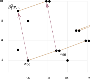
Table 2. $E_{2}^{s,f}(S)$ in degrees $95\leq s\leq 102$, $4\leq f\leq 10$. Brown lines represent $\alpha_{1}$-multiplication. Each dot represents a copy of $\mathbb{F}_{3}$. The information in this chart used in the proof of Lemma 3.4 is summarized in Lemma 3.1(2)(3).

Proof.

By [Rav86, Table A3.4], $\pi_{96}(S)^{\wedge}_{3}=0$, and the generator $x_{96}\in E_{2}^{96,4}(S)$ must support a nontrivial differential as it cannot be a target for degree reasons. We claim this implies a differential $d_{5}(x_{96})=\beta_{1}^{2}x_{75}$: by Lemma 3.1(2) the only other possible target is $\alpha_{1}\beta_{1}^{4}\beta_{2}^{2}\in E_{2}^{95,13}(S)$ (a possibility for $d_{9}(x_{96})$), but this is zero in $E_{6}$ by Lemma 2.5(2) as it is $\alpha_{1}\beta_{1}^{3}$ times the permanent cycle $\beta_{1}\beta_{2}^{2}$.

From Lemma 3.1(2), we have $\alpha_{1}d_{5}(x_{96})=d_{5}(\alpha_{1}x_{96})=\alpha_{1}\beta_{1}^{2}x_{75}$ is nonzero. By [Rav86, Table A3.4], we have $\pi_{99}(S)^{\wedge}_{3}/\operatorname{Im}J\cong\mathbb{F}_{3}$. We claim this permanent cycle is detected in filtration 5. By Lemma 3.1(3), the only other possibility is $\alpha_{1}\beta_{1}^{7}\beta_{2}\in E_{2}^{99,17}(S)$, which is the target of a $d_{5}$ differential by Lemma 2.5(2). Let $x_{99}$ denote the permanent cycle in $E_{2}^{99,5}(S)$. Since $\alpha_{1}^{2}=0$ and $\operatorname{dim}(\alpha_{1}E_{2}^{99,5}(S))=1$ by Lemma 3.1(3), we have that $\alpha_{1}E_{2}^{99,5}(S)$ is generated by $\alpha_{1}x_{99}$. ∎

Lemma 3.5.

The generator of $E_{2}^{142,10}(S)$ supports a nontrivial Adams-Novikov $d_{5}$ differential. The generator of $E_{2}^{142,6}(S)$ supports a nontrivial Adams-Novikov $d_{9}$ differential.

Proof.

Combining Lemma 3.1(5) with Lemma 3.3, we have that the 2-dimensional vector space $E_{2}^{141,15}(S)$ is generated by $\beta_{1}^{6}$-divisible permanent cycles. By Lemma 2.5(1), both classes in $E_{2}^{141,15}(S)$ are hit by some differential. By the vector space structure of $E_{2}^{142,*}(S)$ displayed in Figure 4, the only possibilities are the indicated $d_{5}$ and $d_{9}$. ∎

Lemma 3.6.

The generator of $E_{2}^{143,9}(S)$ supports a nontrivial Adams-Novikov $d_{5}$ differential hitting $\alpha_{1}\beta_{1}^{4}x_{99}$, where $x_{99}$ is the permanent cycle introduced in Lemma 3.4. One of the two generators of $E_{2}^{143,5}(S)$ supports a nontrivial Adams-Novikov $d_{9}$ differential hitting $\beta_{1}^{6}\beta_{6/3}$.

Proof.

This proof relies on Figure 4, in particular the fact that the elements mentioned are all nonzero. For the first statement, we have $d_{5}(\beta_{3/3}\cdot\beta_{1}x_{99})=\alpha_{1}\beta_{1}^{3}\cdot\beta_{1}x_{99}$ since $x_{99}$ (and hence $\beta_{1}x_{99}$) is a permanent cycle. Since $\beta_{6/3}\in E_{2}^{82,2}(S)$ is a permanent cycle by [Rav86, Table A3.4], we may apply Lemma 2.5(1) to show that $\beta_{1}^{6}\beta_{6/3}\in E_{2}^{142,14}(S)$ is the target of a differential $d_{r}$ for $r\leq 9$. Since the group $E_{2}^{143,9}(S)$ is one-dimensional and we proved above that the generator supported a nontrivial $d_{5}$, $\beta_{1}^{6}\beta_{6/3}$ must be hit by a $d_{9}$. ∎

Proposition 3.7.

Every element in $\pi_{143}(S/3)$ is detected in Adams-Novikov filtration $\leq 5$.

Proof.

We list the elements in $E_{2}^{143,f}(S/3)$ for $f>5$.

Filtration $f$	# bottom cell generators	# top cell generators
9	1	1
13	0	2
17	1	0
21	0	1
29	1	0

Table 3. Classes in $E_{2}^{143,f}(S/3)$ for $f\geq 2$

We encourage the reader to refer to Figure 5, which is derived from Figure 4, alongside the rest of the proof.

Filtration 9: We claim that both classes $E_{2}^{143,9}(S/3)$ support $d_{5}$ differentials. The bottom cell class does so because of Lemmas 3.6 and 2.6(1), and the top cell class does so because of Lemma 3.5 and Lemma 2.6(2).

Filtration 13: We may take the two generators of $E_{2}^{143,13}(S/3)$ to be classes ${\overline{\alpha_{1}\beta_{1}^{4}x_{99}}}$ and ${\overline{\beta_{1}^{6}\beta_{6/3}}}$ defined such that their image under $j$ is $\alpha_{1}\beta_{1}^{4}x_{99}$ and $\beta_{1}^{6}\beta_{6/3}$, respectively. By Lemma 2.6(2), the $d_{5}$ in Lemma 3.6 induces a $d_{5}$ differential hitting ${\overline{\alpha_{1}\beta_{1}^{4}x_{99}}}$; note that $\operatorname{Im}(i)=0$ in this degree.

By Lemma 3.6 we have a class $t_{2}\in E_{2}^{143,5}(S)$ such that $d_{9}(t_{2})=\beta_{1}^{6}\beta_{6/3}$. Let ${\overline{t_{2}}}$ be the top cell class in $E_{2}^{144,4}(S/3)$ associated to the 3-torsion element $t_{2}$. We wish to show that there is a differential $d_{9}({\overline{t_{2}}})={\overline{\beta_{1}^{6}\beta_{6/3}}}$. First we check that ${\overline{t_{2}}}$ survives to the $E_{9}$ page. The only possible targets for such a shorter differential are in $E_{2}^{143,9}(S/3)$, and we showed above that these both support nontrivial $d_{5}$ differentials. The map induced by $j$ on $E_{2}$ pages shows that $d_{9}({\overline{t_{2}}})\equiv{\overline{\beta_{1}^{6}\beta_{6/3}}}$ modulo $\ker(j)$. We have $E_{9}^{143,13}(S/3)=\mathbb{F}_{3}\{{\overline{\beta_{1}^{6}\beta_{6/3}}}\}$, and $j({\overline{\beta_{1}^{6}\beta_{6/3}}})=\beta_{1}^{6}\beta_{6/3}$ which is nonzero in $E_{9}(S)$. Thus there is a nonzero $d_{9}$ differential as claimed.

Filtration 17: The generator of $E_{2}^{143,17}(S)$ is $\beta_{1}^{6}\beta_{2}x_{57}$, where $x_{57}$ is the generator of $E_{2}^{57,3}(S)$. Using a differential in Table 1, we have a differential $d_{5}(\beta_{1}^{6}\beta_{2}x_{57})=\beta_{1}^{9}\beta_{2}^{2}$. By Lemma 2.6(1) we have a differential $d_{5}(i(\beta_{1}^{6}\beta_{2}x_{57}))=i(\beta_{1}^{9}\beta_{2}^{2})$.

Filtration 21: By Lemma 2.6(2), the $d_{5}$ differential on $\beta_{1}^{6}\beta_{2}x_{57}$ discussed in the filtration 17 case above gives rise to a differential $d_{5}({\overline{\beta_{1}^{6}\beta_{2}x_{57}}})={\overline{\beta_{1}^{9}\beta_{2}^{2}}}$ over $S/3$.

Filtration 29: The generator of $E_{2}^{143,29}(S/3)$ is $i(\alpha_{1}\beta_{1}^{14})$; this class is zero in $E_{6}(S/3)$ by Lemma 2.5(2). ∎

Remark 3.8.

The dependence of Proposition 3.7 on computer calculations would be reduced if we could make precise the observation that much of the Adams-Novikov $E_{2}$-page is $\beta_{1}$-periodic, and classes in high filtrations are highly $\beta_{1}$-divisible. Using [Pal01, Theorem 2.3.1, Remark 2.3.5(c)], one can prove that multiplication by $\beta_{1}$ is an isomorphism on the Adams $E_{2}$ page restricted to Adams filtration $f_{A}$, stem $s$, and filtration $\nu$ in the algebraic Novikov spectral sequence $\operatorname{Ext}^{*,*}_{A}(\mathbb{F}_{3},\mathbb{F}_{3})\implies E_{2}^{*,*}(S)$ if

$$f_{A}>{\textstyle{1\over 23}}s+{\textstyle{24\over 23}}\nu+{\textstyle{159\over 23}}.$$

By keeping track of the effect on the algebraic Novikov spectral sequence, one can derive that $\beta_{1}$ acts injectively (up to higher algebraic Novikov filtration) on the subspace of $E_{2}^{s,f}(S)$ in algebraic Novikov filtration $\nu$ if

(3.1) $$f>{\textstyle{1\over 23}}s+{\textstyle{1\over 23}}\nu+{\textstyle{169\over 23}}.$$

Surjectivity is harder to prove. Even if we knew that $\beta_{1}$ acted isomorphically on the region (3.1) (which is often true), this is not enough to prove the $\beta_{1}$-divisibility results we need. For example, in Proposition 3.7 we use the fact that the generator $x$ of $E_{2}^{143,17}(S)$ is divisible by $\beta_{1}^{6}$. This element has $\nu=0$, and $\beta_{1}^{-1}x$ and $\beta_{1}^{-2}x$ lie in the region (3.1) but $\beta_{1}^{-3}x$ does not. Improving this bound would also be of use more generally to the study of the 3-primary Adams and Adams-Novikov spectral sequences.

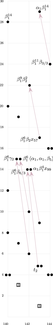
Figure 4. $E_{2}^{s,f}(S)$ in degrees $140\leq s\leq 144$, along with some Adams-Novikov differentials. A box containing “3” denotes a copy of $\mathbb{Z}/27$. Multiplications by $\alpha_{1}$ are not shown.

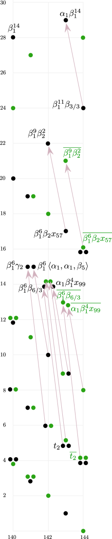
Figure 5. $E_{2}^{s,f}(S/3)$ in degrees $140\leq s\leq 144$, along with some Adams-Novikov differentials. Green dots denote top cell classes. Multiplications by $\alpha_{1}$ are not shown.

4. Survival of $v_{2}^{9}$

In this section, we prove Theorem 4.6, which says that $v_{2}^{9}$ is a permanent cycle in $E_{2}(S/(3,v_{1}^{8}))$. We first explain the choice of exponent of $v_{1}$. Since $\eta_{R}(v_{2})\equiv v_{2}+v_{1}t_{1}^{3}-v_{1}^{3}t_{1}\pmod{3}$ in the Hopf algebroid $(BP_{*},BP_{*}BP)$ (see e.g. [Rav86, (6.4.16)]), we have that $v_{2}^{3}$ is an element of $E_{2}(S/(3,v_{1}^{m}))$ for $m\leq 3$, and $v_{2}^{9}$ is an element of $E_{2}(S/(3,v_{1}^{m}))$ for $m\leq 9$. On the other hand, we would like to work with $m\geq 8$, since those are the values of $m$ for which $\beta_{9/8}$ is in the image of the composition of Adams-Novikov $E_{2}$ page boundary maps $E_{2}(S/(3,v_{1}^{m}))\to E_{2}(S/3)\to E_{2}(S)$. Trivial modifications to the work in this section show that $v_{2}^{9}\pm v_{1}^{8}v_{2}^{7}$ is a self-map on $S/(3,v_{1}^{9})$; see Remark 4.8. However, this slight strengthening is not necessary for our purposes, and we write down our results for $v_{2}^{9}\in\pi_{*}(S/(3,v_{1}^{8}))$ essentially for cosmetic reasons, avoiding the correction term. To obtain the families in Theorem 5.1 other than $\beta_{9t+9/j}$, it suffices to work with $S/(3,v_{1}^{4})$.

The main ingredients for proving Theorem 4.6 are Lemma 3.2 and Proposition 3.7 from the previous section, and the following lemma (below, specialized to our setting) due to the second author. It draws a connection between hidden $v_{1}^{8}$-extensions in $\pi_{*}(S/3)$, and differentials of the minimum length (i.e., $d_{5}$ differentials) in the Adams-Novikov spectral sequence for $S/(3,v_{1}^{8})$.

Lemma 4.1 ([Shi97, Lemma 1.4]).

Let $m\geq 1$. Suppose we have $y\in E_{5}(S/(3,v_{1}^{m}))$ such that $j_{m}(y)$ is a nontrivial permanent cycle in $E_{5}^{s,f}(S/3)$, and let $w$ denote an element in $E_{5}(S/3)$ detecting the product $v_{1}^{m}\cdot\{j_{m}(y)\}\in\pi_{*}(S/3)$. Then there is a differential

$$d_{5}(y)=i_{m}(w)$$

in $E_{5}(S/(3,v_{1}^{m}))$.

In the next lemma we separate out the general strategy used to prove that $v_{2}^{9}$ and other elements in Section 5 are permanent cycles.

Lemma 4.2.

1. Let $x\in E_{2}^{s,f}(S/3)$ for $f\leq 3$ be an element such that $j(x)\in E_{2}^{s-1,f+1}(S)$ is a permanent cycle and $\{j(x)\}\in\pi_{s-1}(S)$ is an essential element of order 3. Furthermore, suppose that $\operatorname{Im}(i:E_{2}^{s,f}(S)\to E_{2}^{s,f}(S/3))$ consists of permanent cycles. Then $x\in E_{2}^{s,f}(S/3)$ is a permanent cycle.

2. Let $x\in E_{2}^{s,f}(S/(3,v_{1}^{m}))$ for $f\leq 3$ be an element such that $j_{m}(x)\in E_{2}^{s-4m-1,f+1}(S/3)$ is a permanent cycle and $\{j_{m}(x)\}$ is an essential element with $v_{1}^{m}\cdot\{j_{m}(x)\}=0\in\pi_{*}(S/3)$. Furthermore, suppose that $\operatorname{Im}(i_{m}:E_{2}^{s,f}(S/3)\to E_{2}^{s,f}(S/(3,v_{1}^{m})))$ consists of permanent cycles. Then $x\in E_{2}^{s,f}(S/(3,v_{1}^{m}))$ is a permanent cycle.

Proof.

We just prove (1), as (2) is analogous. Consider the exact sequences

(4.1) $$E_{2}^{s,f}(S)\overset{3}{\to}E_{2}^{s,f}(S)\overset{i}{\to}E_{2}^{s,f}(S/3)\overset{j}{\to}E_{2}^{s-1,f+1}(S)$$

$$\pi_{s}(S)\overset{3}{\to}\pi_{s}(S)\overset{i}{\to}\pi_{s}(S/3)\overset{j}{\to}\pi_{s-1}(S)\overset{3}{\to}\pi_{s-1}(S)$$

associated to the cofiber sequence $S\overset{3}{\to}S\overset{i}{\to}S/3\overset{j}{\to}S$. (For the first long exact sequence, we are using the fact that $j$ induces the zero map in $BP$-homology.) Suppose that $x\in E_{2}^{s,f}(S/3)$ is an element such that $j(x)$ is a permanent cycle with $3\cdot\{j(x)\}=0$. Then there exists an element $\xi\in\pi_{s}(S/3)$ such that $j(\xi)=\{j(x)\}$. Since $j:S/3\to\Sigma S$ induces a map of Adams-Novikov spectral sequences, the induced map on homotopy $j:\pi_{*}(S/3)\to\pi_{*}(\Sigma S)=\pi_{*-1}(S)$ respects Adams-Novikov filtration; thus $j(x)$ being detected in filtration $f+1$ implies $\xi$ is detected in filtration $\leq f$. The assumption $f\leq 3$ combined with Fact 2.3 implies that $\xi$ is detected in filtration $f$. We may write the detecting element as $x+y$ for some $y\in E_{2}^{s,f}(S/3)$. By the Geometric Boundary Theorem, $j(x+y)$ converges to $j(\xi)$, and we also have that $j(x)$ converges to $j(\xi)$. So $j(y)$ is a boundary. But $j(y)$ has filtration $\leq 4$, so Fact 2.3 implies $j(y)=0$ in $E_{2}(S)$. By (4.1), we have that $y$ is in the image of $i$. By the assumption about $\operatorname{Im}(i)$, $y$ is a permanent cycle, and we have from above that $x+y$ is a permanent cycle. Therefore, $x$ is a permanent cycle. ∎

Lemma 4.3.

The element ${\overline{\beta_{9/8}}}=j_{8}(v_{2}^{9})\in E_{2}^{111,1}(S/3)$ is a permanent cycle.

Proof.

By [Rav86, Table A3.4], there exists $c\in\{\pm 1\}$ such that $x_{106}=\beta_{9/9}+c\beta_{7}\in E_{2}^{106,2}(S)$ is a 3-torsion permanent cycle. Lemma 4.2(1) applies since $E_{2}^{*,1}(S)$ consists of permanent cycles; it implies that ${\overline{\beta_{9/9}}}+c{\overline{\beta_{7}}}=j_{9}(v_{2}^{9})+cj_{1}(v_{2}^{7})\in E_{2}^{107,1}(S/3)$ is a permanent cycle. Hence $v_{1}\cdot(j_{9}(v_{2}^{9})+cj_{1}(v_{2}^{7}))=v_{1}\cdot j_{9}(v_{2}^{9})=j_{8}(v_{2}^{9})$ is a permanent cycle. ∎

Lemma 4.4.

We have $d_{5}(v_{2}^{9})=0$ in $E_{5}^{143,5}(S/(3,v_{1}^{8}))$.

Proof.

Let $x=d_{5}(v_{2}^{9})$. We first consider the image of this differential along the natural map induced by $i^{\prime}_{3}:S/(3,v_{1}^{8})\to S/(3,v_{1}^{3})$. Since $v_{2}^{3}$ is an element of $E_{2}^{48,0}(S/(3,v_{1}^{3}))$, by the Leibniz rule and Theorem 2.4, we have $i^{\prime}_{3}(x)=i^{\prime}_{3}(d_{5}(v_{2}^{9}))=d_{5}((v_{2}^{3})^{3})=3v_{2}^{6}d_{5}(v_{2}^{3})=0$.

Using Lemma 4.3, we have

$$j_{8}(x)=j_{8}(d_{5}(v_{2}^{9}))=d_{5}(j_{8}(v_{2}^{9}))=0$$

in $E_{5}(S/3)=E_{2}(S/3)$. Thus the exact sequence

$$E_{2}^{143,5}(S/3)\overset{i_{8}}{\to}E_{2}^{143,5}(S/(3,v_{1}^{8}))\overset{j_{8}}{\to}E_{2}^{111,1}(S/3)$$

gives $x=i_{8}(y)$ for some $y\in E_{2}^{143,5}(S/3)$.

Consider the commutative diagram of cofiber sequences obtained using Verdier’s axiom:

(4.2)

This implies that $i_{3}=i^{\prime}_{3}\circ i_{8}$; in particular, $i_{3}(y)=i^{\prime}_{3}(i_{8}(y))=i^{\prime}_{3}(x)=0$. By the long exact sequence corresponding to the top row of (4.2), we have that $y$ is $v_{1}^{3}$-divisible. By Lemma 3.2, $y=0$. ∎

Lemma 4.5.

The product $v_{1}^{8}\cdot\{j_{8}(v_{2}^{9})\}$ is zero in $\pi_{*}(S/3)$.

Proof.

Let $w\in E_{5}^{143,f}(S/3)$ be a representative of $v_{1}^{8}\cdot\{j_{8}(v_{2}^{9})\}\in\pi_{143}(S/3)$. By Proposition 3.7, we have $f\leq 5$, and by Fact 2.3, the only possibilities are $f=1,5$. The product $v_{1}^{8}\cdot j_{8}(v_{2}^{9})$ is zero on the $E_{2}$ page, so we must have $f=5$.

By Lemma 4.3, Lemma 4.1 applies to $v_{2}^{9}$; combining this with Lemma 4.4, we have

$$0=d_{5}(v_{2}^{9})=i_{8}(w)$$

in $E_{5}^{143,5}(S/(3,v_{1}^{8}))=E_{2}^{143,5}(S/(3,v_{1}^{8}))$. Thus $w$ is divisible by $v_{1}^{8}$ in $E_{2}^{143,5}(S/3)$. By Lemma 3.2, we must have $w=0$ in $E_{5}^{143,5}(S/3)$. Since $w$ was defined to be an element detecting $v_{1}^{8}\cdot\{j_{8}(v_{2}^{9})\}$, this product is zero in homotopy. ∎

Theorem 4.6.

The element $v_{2}^{9}\in E_{2}^{144,0}(S/(3,v_{1}^{8}))$ is a permanent cycle in the Adams-Novikov spectral sequence computing $\pi_{*}(S/(3,v_{1}^{8}))$.

Proof.

This will follow from applying Lemma 4.2(2) to $v_{2}^{9}$. The first two hypotheses of that lemma are satisfied due to Lemma 4.3 and Lemma 4.5. For the last hypothesis, note that $E_{2}^{144,0}(S/3)$ is generated by $v_{1}^{36}$, which is a permanent cycle. ∎

Corollary 4.7.

For $2\leq m\leq 8$, the class $v_{2}^{9}\in\pi_{144}(S/(3,v_{1}^{m}))$ lifts to a class $v_{2}^{9}\in[S/(3,v_{1}^{m}),S/(3,v_{1}^{m})]_{144}$.

Proof.

Naturality of the map $S/(3,v_{1}^{8})\to S/(3,v_{1}^{m})$ for $m\leq 8$ means that Theorem 4.6 directly implies $v_{2}^{9}\in E_{2}^{144,0}(S/(3,v_{1}^{m}))$ is a permanent cycle. By [Oka79, Theorem 6.1], $R=S/(3,v_{1}^{m})$ is a (homotopy) ring spectrum for $m\geq 2$. Thus the desired self map may be obtained as

$$R \to S\wedge R\overset{v_{2}^{9}\wedge I}{\to}R\wedge R\overset{\mu}{\to}R.\qed$$

Remark 4.8.

Essentially the same argument shows that $v_{2}^{9}\pm v_{1}^{8}v_{2}^{7}$ is a permanent cycle in $E_{2}^{144,0}(S/(3,v_{1}^{9}))$. In the proof of Lemma 4.3 we show $j_{9}(v_{2}^{9})\pm j_{1}(v_{2}^{7})=j_{9}(v_{2}^{9}\pm v_{1}^{8}v_{2}^{7})$ is a permanent cycle. The proofs of Lemmas 4.4 and 4.5 go through without modification to show that $d_{5}(v_{2}^{9}\pm v_{1}^{8}v_{2}^{7})=0$ in $E_{5}^{143,5}(S/(3,v_{1}^{9}))$ and $v_{1}^{9}\cdot\{j_{9}(v_{2}^{9}\pm v_{1}^{8}v_{2}^{7})\}=0$. In the proof of Theorem 4.6, we have $x=c_{1}(v_{2}^{9}\pm v_{1}^{8}v_{2}^{7})+c_{2}v_{2}^{9}+c_{3}v_{1}^{36}$. This time, $v_{2}^{9}$ and $v_{1}^{8}v_{2}^{7}$ are not permanent cycles since $\beta_{9/9}=j(j_{9}(v_{2}^{9}))$ and $\beta_{7}=j(j_{9}(v_{1}^{8}v_{2}^{7}))$ are not permanent cycles, and $v_{1}^{36}$ is a permanent cycle. Thus $v_{2}^{9}\pm v_{1}^{8}v_{2}^{7}$ is a permanent cycle for some choice of sign.

5. Survival of beta elements

Our goal in this section is to prove that several infinite families of $\beta_{a/b}$ elements are permanent cycles in the Adams-Novikov spectral sequence for the sphere. For indices $a,b$ satisfying the conditions in [MRW77, Theorem 2.6], Miller, Ravenel, and Wilson define cycles $\beta_{a/b}$ in $E_{2}^{*,2}(S)$ as the image of certain classes in $E_{2}^{*,0}(S/(3,v_{1}^{b}))$ under the composition $j\circ j_{b}$. In this section we will only consider classes $\beta_{sp^{n}/b}$ (with $p\nmid s$) such that $b\leq p^{n}$, which enables us to use the equivalent, but simpler, definition

$$\beta_{a/b}=j(j_{b}(v_{2}^{a}))\in E_{2}^{16a-4b-2,2}(S)$$

(at $p=3$). These elements are defined using the boundary maps $j$ and $j_{b}$ on $\operatorname{Ext}$ associated to the short exact sequences $BP_{*}\overset{3}{\to}BP_{*}\to BP_{*}/3$ and $BP_{*}/3\overset{v_{1}^{b}}{\to}BP_{*}/3\to BP_{*}/(3,v_{1}^{b})$; by the Geometric Boundary Theorem these coincide with the maps induced on Adams-Novikov spectral sequences by the maps $j$ and $j_{b}$ of spectra that we have been considering in this paper. Recall the convention that $\beta_{a}:=\beta_{a/1}$.

Suppose $\beta_{a/b}$ is a permanent cycle with $b\leq 8$, and in addition, suppose that the corresponding element in homotopy $\beta^{h}_{a/b}\in\pi_{*}(S)$ factors as

(5.1) $$\beta^{h}_{a/b}:S\overset{B_{a/b}}{\longrightarrow}S/(3,v_{1}^{b})\overset{jj_{b}}{\longrightarrow}S$$

for some $B_{a/b}\in\pi_{*}(S/(3,v_{1}^{b}))$. In this case, for $t\geq 1$, Corollary 4.7 allows us to define elements in $\pi_{*}(S)$:

$$\beta^{h}_{9t+a/b}:S\overset{B_{a/b}}{\longrightarrow}S/(3,v_{1}^{b})\overset{(v_{2}^{9})^{t}}{\longrightarrow}S/(3,v_{1}^{b})\overset{jj_{b}}{\longrightarrow}S.$$

We warn that existence of a factorization (5.1) is not automatic, even if $\beta_{a/b}$ is a permanent cycle and such a factorization exists on the level of Adams-Novikov $E_{2}$ pages. Our goal is to show the following, proved at the end of the section.

Theorem 5.1.

For all $t\geq 0$, the classes

$$\beta_{9t+3/j} \text{ for }j=1,2$$

$$\beta_{9t+6/j} \text{ for }j=1,2,3$$

$$\beta_{9t+9/j} \text{ for }j=1,\dots,8$$

$$\alpha_{1}\beta_{9t+3/3}$$

$$\alpha_{1}\beta_{9t+7}$$

are permanent cycles in the Adams-Novikov spectral sequence for the sphere.

Since $\beta_{3/3}$ and $\beta_{7}$ support Adams-Novikov differentials, none of the families in Theorem 5.1 are trivially multiplicative consequences of a different family. Instead, we have $\alpha_{1}\beta_{3/3}\in\left\langle{\alpha_{1},\alpha_{1},\beta_{1}^{3}}\right\rangle$ and $\alpha_{1}\beta_{7}\in\left\langle{\alpha_{1},\alpha_{1},\beta_{1}^{2}\beta_{6/3}}\right\rangle$. As we will see in Section 6, the families $\alpha_{1}\beta_{9t+3/3}$, $\beta_{9t+6/3}$, and $\alpha_{1}\beta_{9t+7}$ have nontrivial image in $\pi_{*}\mathit{tmf}$, along with the family $\beta_{9t+1}$ constructed in [BP04, Corollary 1.2].

Lemma 5.2.

The class $j_{4}(v_{1}^{2}v_{2}^{3})\in E_{2}^{39,1}(S/3)$ is a permanent cycle such that $j(j_{4}(v_{1}^{2}v_{2}^{3}))=\beta_{3/2}\in E_{2}^{38,2}(S)$ and $v_{1}^{4}\cdot\{j_{4}(v_{1}^{2}v_{2}^{3})\}=0$ in $\pi_{*}(S/3)$.

Proof.

We have $j(j_{4}(v_{1}^{2}v_{2}^{3}))=j(j_{2}(v_{2}^{3}))=\beta_{3/2}$ in $E_{2}(S)$ by the definition of the $\beta$ elements along with Lemma 2.7. By classical computations of the Adams-Novikov $E_{2}$ page (see e.g. [Rav86, Figure 1.2.19]), $E_{2}^{38,f}(S)=0=E_{2}^{37,f+1}(S)$ for $f\geq 3$, so $E_{2}^{38,f}(S/3)=0$ for $f\geq 3$. Thus $j_{4}(v_{1}^{2}v_{2}^{3})\in E_{2}^{39,1}(S/3)$ cannot support a differential of any length.

As $v_{1}^{4}\cdot j_{4}=0$ as a map $E_{2}(S/(3,v_{1}^{4}))\to E_{2}(S/3)$, it remains to rule out hidden $v_{1}^{4}$-extensions on $\beta^{\prime}_{3/2}:=\{j_{4}(v_{1}^{2}v_{2}^{3})\}\in\pi_{39}(S/3)$. Using [Rav86, Table A3.4] we have $\pi_{51}(S/3)=\mathbb{F}_{3}\{\alpha_{13},{\overline{\beta_{1}^{5}}}\}$ and so $v_{1}^{3}\cdot\beta^{\prime}_{3/2}=c{\overline{\beta_{1}^{5}}}=c{\overline{\beta_{1}^{2}}}\cdot\beta_{1}^{3}$ for some $c\in\mathbb{F}_{3}$. (If there were an $\alpha_{13}$ component, then the extension would not be hidden.) We have $v_{1}\cdot{\overline{\beta_{1}^{2}}}=0$ for degree reasons, as Ravenel’s table implies $\pi_{25}(S/3)=0$. Thus $v_{1}\cdot v_{1}^{3}\cdot\beta^{\prime}_{3/2}=0$. ∎

Lemma 5.3.

The class $j_{4}(v_{1}v_{2}^{6})\in E_{2}^{83,1}(S/3)$ is a permanent cycle such that $j(j_{4}(v_{1}v_{2}^{6}))=\beta_{6/3}\in E_{2}^{82,2}(S)$ and $v_{1}^{4}\cdot\{j_{4}(v_{1}v_{2}^{6})\}=0$ in $\pi_{*}(S/3)$.

Proof.

By Ravenel’s table [Rav86, Table A3.4], $\beta_{6/3}$ and $\beta_{6}$ are 3-torsion permanent cycles. Since $j(j_{4}(v_{1}v_{2}^{6}))=\beta_{6/3}$ and $j(j_{4}(v_{1}^{3}v_{2}^{6}))=\beta_{6}$, we apply Lemma 4.2(1) to $j_{4}(v_{1}v_{2}^{6})\in E_{2}^{83,1}(S/3)$ and $j_{4}(v_{1}^{3}v_{2}^{6})\in E_{2}^{91,1}(S/3)$, noting that $E_{2}^{*,1}(S)$ consists of permanent cycles. This shows that $j_{4}(v_{1}v_{2}^{6})$ and $j_{4}(v_{1}^{3}v_{2}^{6})$ are permanent cycles.

To determine $v_{1}^{4}\cdot\{j_{4}(v_{1}v_{2}^{6})\}$, we first consider the possibilities for $v_{1}^{2}\cdot\{j_{4}(v_{1}v_{2}^{6})\}\in\pi_{91}(S/3)$: from Ravenel’s tables, we have

$$\pi_{91}(S/3)=\mathbb{F}_{3}\{\alpha_{23},\beta_{1}\gamma_{2},\beta_{1}x_{81},\beta^{\prime}_{6}\}$$

where $j(\beta^{\prime}_{6})=\beta_{6}$. Since $v_{1}^{2}\cdot\beta_{1}=0$ in homotopy by Lemma 2.5(3), we have $v_{1}^{2}\cdot\{j_{4}(v_{1}v_{2}^{6})\}=c_{1}\alpha_{23}+c_{2}\beta^{\prime}_{6}$ for $c_{i}\in\mathbb{F}_{3}$. If $c_{1}\neq 0$ then $v_{1}^{4}\cdot\{j_{4}(v_{1}v_{2}^{6})\}$ would be detected in filtration 1, contradicting the fact that $v_{1}^{4}\cdot j_{4}(v_{1}v_{2}^{6})=0$ in $E_{2}(S/3)$. So it suffices to show that $v_{1}^{2}\cdot\beta^{\prime}_{6}=0$. From above, we may write $\beta^{\prime}_{6}=\{j_{4}(v_{1}^{3}v_{2}^{6})\}=\{j_{2}(v_{1}v_{2}^{6})\}$. By [Oka81, Lemma 3], $v_{1}v_{2}^{6}\in E_{2}^{100,0}(S/(3,v_{1}^{2}))$ is a permanent cycle, and hence so is $j_{2}(v_{1}v_{2}^{6})$. We have $\{j_{2}(v_{1}v_{2}^{6})\}=j_{2}(\{v_{1}v_{2}^{6}\})$ by the Geometric Boundary theorem, and $v_{1}^{2}\cdot j_{2}(\{v_{1}v_{2}^{6}\})=0$ by definition of $j_{2}$ as a map on homotopy groups. ∎

Lemma 5.4.

The classes $v_{1}^{2}v_{2}^{3}\in E_{2}^{56,0}(S/(3,v_{1}^{4}))$ and $v_{1}v_{2}^{6}\in E_{2}^{100,0}(S/(3,v_{1}^{4}))$ are permanent cycles in the Adams-Novikov spectral sequence computing $\pi_{*}(S/(3,v_{1}^{4}))$.

Proof.

Use Lemma 4.2(2), with Lemmas 5.2 and 5.3 as input. To check the condition about the image of $i_{4}:E_{2}(S/3)\to E_{2}(S/(3,v_{1}^{4}))$ in these degrees, note that $E_{2}^{*,1}(S/3)$ is generated by the image of $i:E_{2}^{*,1}(S)\to E_{2}^{*,1}(S/3)$, which consists of permanent cycles (these are all image of $J$ classes), along with elements that map to $\beta$ elements under $j$. Standard theory about the $\beta$ elements ([MRW77]) implies that ${\overline{\beta_{3/2}}}$ and ${\overline{\beta_{6/3}}}$ are the only such elements in the relevant degrees; these are both permanent cycles by Lemmas 5.2 and 5.3. ∎

Lemma 5.5.

The class $\alpha_{1}v_{1}v_{2}^{3}\in E_{2}^{55,1}(S/(3,v_{1}^{4}))$ is a permanent cycle in the Adams-Novikov spectral sequence.

Proof.

There is a Toda bracket $\left\langle{\alpha_{1},\alpha_{1},\beta_{1}^{3}}\right\rangle\in\pi_{37}(S)$ detected by $\alpha_{1}\beta_{3/3}$ in filtration 3, and this class is 3-torsion (see [Rav86, Table A3.4]). In order to apply Lemma 4.2(1) to $j_{4}(\alpha_{1}v_{1}v_{2}^{3})\in E_{2}^{38,2}(S/3)$, we must check that $E_{2}^{38,2}(S)$ consists of permanent cycles. It follows from standard facts about the Adams-Novikov 2-line ([MRW77]) that $E_{2}^{38,2}(S)=\mathbb{F}_{3}\{\beta_{3/2}\}$. So we may conclude that $j_{4}(\alpha_{1}v_{1}v_{2}^{3})$ is a permanent cycle.

Moreover, $v_{1}^{4}\cdot\{j_{4}(\alpha_{1}v_{1}v_{2}^{3})\}$ is zero in homotopy: since $\pi_{53}(S)=0=\pi_{54}(S)$ by [Rav86, Table A3.4], we have $\pi_{54}(S/3)=0$. In order to apply Lemma 4.2(2) to $\alpha_{1}v_{1}v_{2}^{3}\in E_{2}^{55,1}(S/(3,v_{1}^{4}))$, we must check that $E_{2}^{55,1}(S/3)$ consists of permanent cycles. This is true because the image of $E_{2}^{*,1}(S)$ consists of permanent cycles, and analysis of the 2-line reveals that there cannot be a class with nontrivial image in $E_{2}^{54,2}(S)$. Thus we have that $\alpha_{1}v_{1}v_{2}^{3}$ is a permanent cycle. ∎

Lemma 5.6.

The class $\alpha_{1}v_{1}v_{2}^{7}\in E_{2}^{119,1}(S/(3,v_{1}^{2}))$ is a permanent cycle in the Adams-Novikov spectral sequence.

Proof.

Since $S/(3,v_{1}^{2})$ is a ring spectrum (Theorem 2.4), we may consider this element as a product $v_{1}v_{2}^{5}\cdot\alpha_{1}v_{2}^{2}$. Oka [Oka81, Lemma 2] showed that $v_{2}^{5}$ is a permanent cycle in $E_{2}^{80,0}(S/(3,v_{1}))$. This implies that $v_{1}v_{2}^{5}$ is a permanent cycle in $E_{2}^{84,0}(S/(3,v_{1}^{2}))$.

Next we consider possible differentials on $\alpha_{1}v_{2}^{2}\in E_{2}^{35,1}(S/(3,v_{1}^{2}))$. An element in $E_{2}^{34,f}(S/(3,v_{1}^{2}))$ either has nonzero image under $j_{2}$ in $E_{2}^{25,f+1}(S/3)$ or is the image under $i_{2}$ of an element of $E_{2}^{34,f}(S/3)$. From classically known computations of the Adams-Novikov $E_{2}$ page (e.g. see [Rav86, Figure 1.2.19]), we deduce that $E_{2}^{25,*}(S/3)=0$ and $E_{2}^{35,\geq 3}(S/3)=\mathbb{F}_{3}\{{\overline{\alpha_{1}\beta_{1}^{3}}}\}$. This implies $E_{2}^{34,\geq 3}(S/(3,v_{1}^{2}))$ is generated by $i_{2}({\overline{\alpha_{1}\beta_{1}^{3}}})$. Observe that ${\overline{\alpha_{1}\beta_{1}^{3}}}={\overline{\alpha_{1}}}\beta_{1}^{3}=v_{1}\cdot\beta_{1}^{3}$. Thus the only possible nonzero differential on $v_{1}v_{2}^{5}\cdot\alpha_{1}v_{2}^{2}$ is a $d_{5}$ with target $v_{1}v_{2}^{5}\cdot v_{1}\beta_{1}^{3}$. But the target is divisible by $v_{1}^{2}$, hence zero in $E_{5}(S/(3,v_{1}^{2}))$. ∎

Proof of Theorem 5.1.

We show that $\beta_{9t+3/2}$ and $\beta_{9t+3/1}$ are permanent cycles for $t\geq 0$. Since $v_{2}^{9}$ is a permanent cycle in $E_{2}(S/(3,v_{1}^{8}))$ by Theorem 4.6, its image in $E_{2}(S/(3,v_{1}^{4}))$ is a permanent cycle. Lemma 5.4 says that $v_{1}^{2}v_{2}^{3}$ is a permanent cycle in $E_{2}(S/(3,v_{1}^{4}))$, so the product $v_{1}^{2}v_{2}^{3}\cdot v_{2}^{9t}\in E_{2}(S/(3,v_{1}^{4}))$ is a permanent cycle. Recall that $\beta_{9t+3/2}\in E_{2}(S)$ is defined as $j(j_{2}(v_{2}^{9t+3}))=j(j_{4}(v_{1}^{2}v_{2}^{9t+3}))$ in $E_{2}(S/3)$. Since $j_{4}(v_{1}^{2}v_{2}^{9t+3})$ is a permanent cycle, so is $j(j_{4}(v_{1}^{2}v_{2}^{9t+3}))$. Since $v_{1}^{2}v_{2}^{3}$ is a permanent cycle in $E_{2}(S/(3,v_{1}^{4}))$, so is $v_{1}^{3}v_{2}^{3}$, so $\beta_{9t+3/1}=j(j_{1}(v_{2}^{9t+3}))=j(j_{4}(v_{1}^{3}v_{2}^{9t+3}))$ is a permanent cycle in $E_{2}(S)$.

The family $\beta_{9t+9/8}$ (and hence $\beta_{9t+9/j}$ for $j<8$) follows directly from the fact that $v_{2}^{9}$ is a permanent cycle in $E_{2}(S/(3,v_{1}^{8}))$. The other families of permanent cycles follow analogously, using Lemma 5.4 again as the input for $\beta_{9t+6/3}=j(j_{4}(v_{1}v_{2}^{9t+6}))$, Lemma 5.5 as the input for $\alpha_{1}\beta_{9t+3/3}=j(j_{4}(\alpha_{1}v_{1}v_{2}^{9t+3}))$, and Lemma 5.6 as the input for $\alpha_{1}\beta_{9t+7}=j(j_{2}(\alpha_{1}v_{1}v_{2}^{9t+7}))$. ∎

6. 3-primary Hurewicz image of $\mathit{tmf}$

In this section we determine the image of the Hurewicz map $h:\pi_{*}S\to\pi_{*}\mathit{tmf}$ induced by the unit map $S\to\mathit{tmf}$. The target $\pi_{*}\mathit{tmf}$ has been computed via the elliptic spectral sequence (see [Bau08, §3]); this is the $Y(4)$-based Adams spectral sequence for $\mathit{tmf}$, where $Y(4)$ is the Thom spectrum of $\Omega U(4)\to\mathbb{Z}\times BU$. We will denote this spectral sequence by $E^{\textit{ell}}_{r}(\mathit{tmf})$.

Theorem 6.1 (Hopkins-Mahowald, Bauer [Bau08, §6]).

At $p=3$, $\pi_{*}\mathit{tmf}$ is generated by $c_{4}$, $c_{6}$, $\Delta$, $\alpha$, $\beta$, and $b$, subject to the relation $c_{4}^{3}-c_{6}^{2}=1728\Delta$ and the relations on the other generators displayed in Figure 6. Multiplication by $\Delta^{3}\in\pi_{72}(\mathit{tmf})$ is injective.

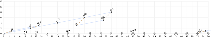
Figure 6. The $E_{\infty}$ page of the elliptic spectral sequence computing $\pi_{s}\mathit{tmf}$ for $0\leq s\leq 76$. Dashed brown lines represent hidden $\alpha$-multiples. Squares indicate copies of $\mathbb{Z}_{(3)}$ and dots indicate copies of $\mathbb{F}_{3}$.

We will show (Theorem 6.5) that all classes in filtration $\geq 2$ are in the Hurewicz image, and the only classes in filtrations 0 and 1 in the image are the summands generated by $1$ and $\alpha$. Instead of directly mapping to the elliptic spectral sequence, we use the $K(2)$-local $E$-based Adams spectral sequence

$$E^{E}_{2}(\mathit{TMF})=H^{*}(G_{24};E_{*})\implies\pi_{*}(L_{K(2)}\mathit{TMF})$$

where $E=E_{2}$ is height 2 Morava $E$-theory and $\mathit{TMF}$ is the periodic version of $\mathit{tmf}$. There is a map of spectral sequences $E_{r}(S)\to E^{E}_{r}(\mathit{TMF})$ induced by the natural maps $BP\to E$ and $S\to\mathit{TMF}$. Henn-Karamanov-Mahowald [HKM13, Theorem 1.1] completely determine $E^{E}_{2}(\mathit{TMF}/3)$ and provide formulas that we use to compute the map on $E_{2}$ pages $E_{2}(S)\to E^{E}_{2}(\mathit{TMF})$ in cases of interest (see Lemmas 6.2 and 6.3). For each class in $E^{E}_{2}(\mathit{TMF})$ in filtration $\geq 2$, we identify a preimage in $E_{2}(S)$ that is among the classes proved to be permanent cycles in Theorem 5.1 or [BP04] (see Proposition 6.4). As we explain in the proof of Theorem 6.5, it suffices to understand the Hurewicz image in $\pi_{*}(L_{K(2)}\mathit{TMF})$ because there is an injection $\pi_{*}(\mathit{tmf})\to\pi_{*}(L_{K(2)}\mathit{TMF})$ (see Lemma 6.6).

First we review some notation and basic facts. We have $E_{*}/3=\mathbb{F}_{9}[[u_{1}]][u^{\pm 1}]$, and there is a natural map $BP_{*}\to E_{*}$ that sends $v_{1}\mapsto u_{1}u^{-2}$, $v_{2}\mapsto u^{-8}$, and $v_{i}\mapsto 0$ for $i>2$. Abusing notation, we will let $v_{i}$ denote its image in $E_{*}/3$.

Recall $j:S/3\to\Sigma S$ denotes the boundary map in the cofiber sequence $S\overset{3}{\to}S\to S/3$. We will also use $j$ to refer to the map $j\wedge\mathit{TMF}:\mathit{TMF}/3\to\Sigma\mathit{TMF}$. Similarly, $j_{m}$ will denote both boundary maps $S/(3,v_{1}^{m})\to S/3$ and $\mathit{TMF}/(3,v_{1}^{m})\to\mathit{TMF}/3$ depending on context.

Lemma 6.2.

In $E_{*}$ we have

$$v_{2}^{3} \equiv-\Delta^{2}-v_{1}^{2}v_{2}\Delta\pmod{(3,v_{1}^{6})}$$

$$v_{2}^{6} \equiv\Delta^{4}-v_{1}^{2}v_{2}\Delta^{3}\pmod{(3,v_{1}^{3})}$$

$$v_{2}^{3^{n}} \equiv-\Delta^{2\cdot 3^{n-1}}-v_{1}^{2\cdot 3^{n-1}}v_{2}^{3^{n-1}}\Delta^{3^{n-1}}\pmod{(3,v_{1}^{2\cdot 3^{n}})}.$$

Proof.

The formula $\Delta\equiv(1-\omega^{2}u_{1}^{2}+u_{1}^{4})\omega^{2}u^{-12}\pmod{(3,u_{1}^{6})}$ from [HKM13, Proposition 5.1] implies

$$\Delta^{2} \equiv(1-2\omega^{2}u_{1}^{2}+u_{1}^{4})(-v_{2}^{3})\pmod{(3,v_{1}^{6})}$$

$$v_{1}^{2}v_{2}\Delta \equiv v_{2}^{3}(\omega^{2}u_{1}^{2}+u_{1}^{4})\pmod{(3,v_{1}^{6})}.$$

where $\omega$ denotes an $8^{th}$ root of unity in $\mathbb{F}_{9}$. Combining these facts, we obtain the formula for $v_{2}^{3}$; the formulas for $v_{2}^{6}$ and $v_{2}^{3^{n}}$ follow from it by squaring and successive cubing, respectively. ∎

Let

$$H :E_{2}(S)\to E^{E}_{2}(\mathit{TMF})$$

$$H^{\prime} :E_{2}(S/3)\to E^{E}_{2}(\mathit{TMF}/3)$$

$$H^{\prime}_{m} :E_{2}(S/(3,v_{1}^{m}))\to E^{E}_{2}(\mathit{TMF}/(3,v_{1}^{m}))$$

denote the natural maps of spectral sequences.

Lemma 6.3.

We have

$$H(\alpha_{1}) =\alpha H^{\prime}(j_{3}(v_{2}^{3})) \doteq\Delta\widetilde{\alpha} H^{\prime}(j_{3}(v_{1}^{2}v_{2}^{7})) \doteq\Delta^{4}\widetilde{\alpha}$$

$$H(\beta_{1}) \doteq\beta H(\beta_{3/3}) \doteq\Delta\beta H(\beta_{7}) \doteq\Delta^{4}\beta$$

$$H^{\prime}(j_{3}(v_{1}^{2}v_{2})) \doteq\widetilde{\alpha} H^{\prime}(j_{3}(v_{2}^{6})) \doteq\Delta^{3}\widetilde{\alpha}$$

$$H(\beta_{6/3}) \doteq\Delta^{3}\beta$$

where $j(\widetilde{\alpha})=\beta$. (Here $\doteq$ denotes equality up to multiplication by a unit.)

Proof.

Following Bauer [Bau08, §6], we have $H(\alpha_{1})=\alpha$ since they both come from the cobar class $[t_{1}]$, and $H(\beta_{1})=\beta$ because of the Massey products $\beta_{1}=\left\langle{\alpha_{1},\alpha_{1},\alpha_{1}}\right\rangle$ and $\beta=\left\langle{\alpha,\alpha,\alpha}\right\rangle$. We have $j(\widetilde{\alpha})=\beta$ and $j(j_{3}(v_{1}^{2}v_{2}))=\beta_{1}$, so $j(H^{\prime}(j_{3}(v_{1}^{2}v_{2})))=H(j(j_{3}(v_{1}^{2}v_{2})))=\beta$. This specifies $H^{\prime}(j_{3}(v_{1}^{2}v_{2}))$ up to the image of $E^{E}_{2}(\mathit{TMF})$, but $E^{E}_{2}(\mathit{TMF}/3)$ is 1-dimensional in the degree of $\widetilde{\alpha}$, so there is no ambiguity.

For the next column, we have in $E^{E}_{2}(\mathit{TMF}/(3,v_{1}^{3}))$ that

$$H^{\prime}(j_{3}(v_{2}^{3})) =j_{3}(H^{\prime}_{3}(v_{2}^{3}))=j_{3}(-\Delta^{2}-v_{1}^{2}v_{2}\Delta)=-\Delta j_{3}(v_{1}^{2}v_{2})=-\Delta\cdot\widetilde{\alpha}$$

using Lemma 6.2 and the earlier fact about $H^{\prime}(j_{3}(v_{1}^{2}v_{2}))$. Note that $j_{3}(\Delta^{n})=0$ since $\Delta^{n}$ is in the image of $E^{E}_{2}(\mathit{TMF}/3)$. Now apply $j$ to get the statement about $H(\beta_{3/3})$. The remaining facts in this column are analogous, using the fact that $\beta_{6/3}=j(j_{3}(v_{2}^{6}))$. The last column is also proved similarly, using the fact that $\beta_{7}=j(j_{3}(v_{1}^{2}v_{2}^{7}))$. ∎

By our convention about naming elements in the image of the map $BP_{*}\to E_{*}$, we have $H^{\prime}_{3}(v_{2})=v_{2}$.

Proposition 6.4.

For $t\geq 0$ the map $H:E_{2}(S)\to E^{E}_{2}(\mathit{TMF})$ satisfies:

1. $H(\beta_{9t+1})\doteq\Delta^{6t}\beta$

2. $H(\beta_{9t+3/3})\doteq\Delta^{6t+1}\beta$

3. $H(\beta_{9t+6/3})\doteq\Delta^{6t+3}\beta$

4. $H(\beta_{9t+7})\doteq\Delta^{6t+4}\beta$.

Proof.

These statements are all proved the same way; we show (2). First observe that Lemma 6.2 implies $v_{2}^{9}\equiv-\Delta^{6}\pmod{(3,v_{1}^{6})}$. Using Lemma 6.2 and Lemma 6.3 we have:

$$H(\beta_{9t+3/3}) =H(j(j_{3}(v_{2}^{9t+3})))=j(j_{3}(H^{\prime}_{3}(v_{2}^{9t+3})))$$

$$=j(j_{3}(H^{\prime}_{3}(v_{2}^{3})\cdot H^{\prime}_{3}(v_{2}^{9t})))=j(j_{3}((-\Delta^{2}-v_{1}^{2}v_{2}\Delta)\cdot(-1)^{t}\Delta^{6t}))$$

$$=j(j_{3}((-1)^{t+1}\Delta^{6t+2}))+j(j_{3}((-1)^{t+1}v_{1}^{2}v_{2}\Delta^{6t+1}))$$

$$=0+(-1)^{t+1}\Delta^{6t+1}j(j_{3}(v_{1}^{2}v_{2}))=(-1)^{t+1}\Delta^{6t+1}\beta.$$

In the last line we are using the fact that $j_{3}(v_{1}^{2}v_{2})=\widetilde{\alpha}$ in $E_{2}^{E}(\mathit{TMF}/3)$ from Lemma 6.3. ∎

In the next theorem, we show that every element in $\pi_{*}\mathit{tmf}$ detected in filtration $\geq 2$ is in the Hurewicz image. This result is stated without proof in [Hen14, §1], but we do not know of any prior proof in the literature.

Theorem 6.5.

The image of the map $h:\pi_{*}S\to\pi_{*}\mathit{tmf}$ at $p=3$ consists of the $\mathbb{Z}_{(3)}$ summand generated by 1 and the $\mathbb{F}_{3}$ summands generated by

$$\alpha,\ \Delta^{3t}\beta^{i}\text{ for }1\leq i\leq 4,\ \Delta^{3t}\alpha\beta,\ \Delta^{3t}\beta b$$

for $t\geq 0$. More precisely, we have

$$h(\alpha_{1}) =\alpha$$

$$h(\beta_{1}^{i-1}\beta_{9t+1}) =\Delta^{6t}\beta^{i}\text{ for }1\leq i\leq 4$$

$$h(\alpha_{1}\beta_{9t+3/3}) =\Delta^{6t}\beta b$$

$$h(\beta_{1}^{i-1}\beta_{9t+6/3}) =\Delta^{6t+3}\beta^{i}\text{ for }1\leq i\leq 4$$

$$h(\alpha_{1}\beta_{9t+7}) =\Delta^{6t+3}\beta b.$$

Proof.

Let $E^{\textit{ell}}_{2}(\mathit{tmf})$ denote the elliptic spectral sequence for $\mathit{tmf}$ (see [Bau08, §6]); recall this is the $Y(4)$-based Adams spectral sequence for $\mathit{tmf}$. There is a map of spectral sequences $L:E^{\textit{ell}}_{r}(\mathit{tmf})\to E^{E}_{r}(\mathit{TMF})$ that comes from the map on Adams towers induced by the maps $Y(4)\to MU_{P}\to E$ (where $MU_{P}$ denotes periodic $MU$) and $\mathit{tmf}\to\mathit{TMF}$. These maps assemble into a diagram of spectral sequences as follows.

(6.1)

No element $x\in{E^{\textit{ell}}_{\infty}}^{s,0}(\mathit{tmf})$ for $s\neq 0$ is in the image of $h$: Lemma 6.6(2) implies $x$ would be detected in filtration 0 of $E^{E}_{\infty}(\mathit{TMF})$, and $H:E_{\infty}(S)\to E^{E}_{\infty}(\mathit{TMF})$ is zero in filtration 0 for nonzero stems.

Next we turn to elements detected in filtration 1. We have $H(\alpha_{1})=\alpha$ by Lemma 6.3; since we have $H=L\circ h$ as maps $\pi_{*}S\to\pi_{*}L_{K(2)}\mathit{TMF}$ and $L$ is injective by Lemma 6.6, this implies $h(\alpha_{1})=\alpha\in\pi_{*}\mathit{tmf}$. The other elements of $E^{\textit{ell}}_{\infty}(\mathit{tmf})$ in filtration 1 are $\Delta^{3t}\alpha$ for $t\geq 1$ and $\Delta^{3t}b$ for $t\geq 0$; we will show that the permanent cycles they represent are not in the Hurewicz image. By Lemma 6.6(1) they are in the image of $h$ if and only if their images in $\pi_{*}L_{K(2)}\mathit{TMF}$ are in the image of $H$. By Lemma 6.6(2) they are also detected in filtration 1 in $E^{E}_{\infty}(\mathit{TMF})$, so if they were in the image of $H$, they would be the image of a class in $E_{2}(S)$ in filtration 0 or 1. We have $E_{2}^{s,0}(S)=0$ for $s>1$, so it suffices to show that the elements in $E_{2}^{s,1}(S)$ except for $\alpha_{1}$ are in the kernel of $h$. If $x\in E_{2}^{s,1}(S)$ with $s>3$ then $i(x)=\alpha_{1}v_{1}^{k}$ for some $k\geq 1$. If $h^{\prime}$ denotes the map $\pi_{*}(S/3)\to\pi_{*}(\mathit{tmf}/3)$ induced by $h$, we have $h^{\prime}(\alpha_{1}v_{1})=0$ since $\pi_{7}(\mathit{tmf}/3)=0$. Thus $i(h(x))=h^{\prime}(i(x))=0$ in $\pi_{*}(S/3)$, which implies that $h(x)$ is 3-divisible. But Figure 6 shows that there are no 3-divisible nonzero targets in Adams-Novikov filtration 1.

We will now show how to use Proposition 6.4 to derive the remaining claims about $h$; for multiplicative reasons, it suffices to show $i=1$ in those statements. We will illustrate this with the element $\alpha_{1}\beta_{9t+3/3}$; the other elements are analogous, using Theorem 5.1 for $\beta_{9t+6/3}$ or [BP04, Corollary 1.2] for $\beta_{9t+1}$ in place of Theorem 5.1 below as necessary. By Proposition 6.4, $H(\alpha_{1}\beta_{9t+3/3})=\Delta^{6t+1}\alpha\beta$ in $E^{E}_{2}(\mathit{TMF})$. Since $\Delta^{6t+1}\alpha\beta$ is a permanent cycle in $E^{\textit{ell}}_{2}(\mathit{tmf})$ converging to $\Delta^{6t}\beta b$, we have that $\Delta^{6t+1}\alpha\beta$ is a permanent cycle in $E^{E}_{2}(\mathit{TMF})$ converging to $\Delta^{6t}\beta b$. Theorem 5.1 shows that $\alpha_{1}\beta_{9t+3/3}$ is a permanent cycle in the Adams-Novikov spectral sequence; write $\alpha_{1}\beta_{9t+3/3}$ for the (non-$\alpha_{1}$-divisible) element in homotopy it converges to. The following diagram summarizes these statements by illustrating (6.1) applied to these elements.

Thus $H:\pi_{*}S\to\pi_{*}L_{K(2)}\mathit{TMF}$ satisfies $H(\alpha_{1}\beta_{9t+3/3})=\Delta^{6t}\beta b$. Since $H$ factors through $h$ and $L:\pi_{*}\mathit{tmf}\to\pi_{*}L_{K(2)}\mathit{TMF}$ is injective by Lemma 6.6(1), we have that $h(\alpha_{1}\beta_{9t+3/3})=\Delta^{6t}\beta b$. ∎

Lemma 6.6.

1. The map $L:\pi_{*}\mathit{tmf}\to\pi_{*}L_{K(2)}\mathit{TMF}$ is injective on the classes in Theorem 6.5.

2. The map $L:E^{\textit{ell}}_{\infty}(\mathit{tmf})\to E^{E}_{\infty}(\mathit{TMF})$ is injective in filtration 0 and 1.

In fact, $L$ is injective on $E_{\infty}$ pages in all filtrations, but we do not need this fact.

Proof.

(1) We have

$$\pi_{*}(L_{K(2)}\mathit{TMF})=\left(\pi_{*}(\mathit{tmf})[(\Delta^{3})^{-1}]\right)^{\wedge}_{I}$$

where $I=(3,c_{4})$ (see [Hen14, §2]). It is clear from the calculation of $\pi_{*}\mathit{tmf}$ that the localization map $\pi_{*}(\mathit{tmf})\to(\Delta^{3})^{-1}\pi_{*}(\mathit{tmf})$ is an injection. It suffices to show that completion at $I$ is injective on the specified classes. This holds because $0=c_{4}\cdot\alpha=c_{4}\cdot\beta=c_{4}\cdot b$ in $(\Delta^{24})^{-1}\pi_{*}\mathit{tmf}$ for degree reasons (and these classes are also all 3-torsion).

(2) Consider an element of $\ker(L:E^{\textit{ell}}_{\infty}(\mathit{tmf})\to E^{E}_{\infty}(\mathit{TMF}))$ represented by $x\in E^{\textit{ell}}_{2}(\mathit{tmf})$ in filtration 0 or 1. We claim that $x$ is in $\ker(L_{2}:E^{\textit{ell}}_{2}(\mathit{tmf})\to E^{E}_{2}(\mathit{TMF}))$: since $L_{2}(x)$ is in filtration 0 or 1, it cannot be the target of a $d_{r}$ differential for $r\geq 2$. By comparing the calculations of $E^{\textit{ell}}_{2}(\mathit{tmf})$ and $E^{E}_{2}(\mathit{TMF}/3)$ in [Bau08, §5] and [HKM13, Theorem 1.1], respectively, it is clear that $L^{\prime}_{2}:E^{\textit{ell}}_{2}(\mathit{tmf}/3)\to E^{E}_{2}(\mathit{TMF}/3)$ is an injection, so the image of $x$ in $E^{\textit{ell}}_{2}(\mathit{tmf}/3)$ is zero, which implies (using exactness of the top row in the diagram) $x\in E^{\textit{ell}}_{2}(\mathit{tmf})$ is 3-divisible.

Since $E_{2}^{\textit{ell}}(\mathit{tmf})$ has no 3-divisible classes in filtration 1, we now focus on the filtration 0 case. Let $y=x/3^{n}\in E^{\textit{ell}}_{2}(\mathit{tmf})$ be the non-3-divisible generator, which then has nonzero image $i(y)$ in $E^{\textit{ell}}_{2}(\mathit{tmf}/3)$. Since $L^{\prime}_{2}$ is an injection, $L^{\prime}_{2}(i(y))=i(L_{2}(y))\neq 0$. We claim that the (nonzero) group generated by $L_{2}(y)$ is torsion-free: if not, then the corresponding top cell class would be a nonzero class in $E^{E}_{2}(\mathit{TMF}/3)$ in filtration $-1$, contradicting [HKM13, Theorem 1.1]. So $L_{2}(x)=3^{n}L_{2}(y)\neq 0$, contradicting the fact above that $x\in\ker(L_{2})$. ∎

Remark 6.7.

Our methods are not sufficient to completely determine the image of the map $h^{\prime}:\pi_{*}(S/3)\to\pi_{*}(\mathit{tmf}/3)$. The remaining nontrivial part of this question is to determine which elements $\Delta^{n}\alpha$ are in the image. Arguments similar to those we have given in this section show that $h^{\prime}({\overline{\beta_{9t+2}}})=\Delta^{6t+1}\alpha$ and $h^{\prime}({\overline{\beta_{9t+5}}})=\Delta^{6t+3}\alpha$. However, the families $\Delta^{6t}\alpha$ for $t\geq 1$ and $\Delta^{6t+4}\alpha$ for $t\geq 0$ fit into patterns that are not described by our work in this paper. For example, $\Delta^{4}\alpha\in\pi_{99}(\mathit{tmf}/3)$ is not in the image of $h^{\prime}$ for degree reasons. On the other hand, using the more precise definitions of the $\beta$ elements in [MRW77, (2.4)] and calculating analogously to Lemma 6.3, we find that the map $E_{2}(S/3)\to E^{E}_{2}(\mathit{TMF}/3)$ sends ${\overline{\beta_{18/11}}}$ to $\Delta^{10}\alpha$. As we do not know if ${\overline{\beta_{18/11}}}$ is a permanent cycle, we are unable to conclude whether $\Delta^{10}\alpha$ is in the image of $\pi_{*}(S/3)$.

References

[Bau08]Tilman Bauer
“Computation of the homotopy of the spectrum tmf”
In Groups, homotopy and configuration spaces13, Geom. Topol. Monogr.
Geom. Topol. Publ., Coventry, 2008, pp. 11–40
DOI: 10.2140/gtm.2008.13.11
[BMQ20]Mark Behrens, Mark Mahowald and J. D. Quigley
“The 2-primary Hurewicz image of tmf”, 2020
[BP04]Mark Behrens and Satya Pemmaraju
“On the existence of the self map on the
Smith-Toda complex at the prime 3”
In Homotopy theory: relations with algebraic geometry, group
cohomology, and algebraic -theory346, Contemp. Math.
Amer. Math. Soc., Providence, RI, 2004, pp. 9–49
DOI: 10.1090/conm/346/06284
[Goe07]Paul Goerss
“The Adams-Novikov Spectral Sequence and the Homotopy Groups
of Spheres” Notes from lectures at IRMA Strasbourg, May 7-11, 2007, 2007
[Hen14]André G. Henriques
“The homotopy groups of tmf and of its localizations”
In Topological Modular FormsAmerican Mathematical Society, 2014, pp. 189–205
DOI: 10.1090/surv/201/13
[HKM13]Hans-Werner Henn, Nasko Karamanov and Mark Mahowald
“The homotopy of the -local Moore spectrum at the
prime 3 revisited”
In Math. Z.275.3-4, 2013, pp. 953–1004
DOI: 10.1007/s00209-013-1167-4
[MRW77]Haynes R. Miller, Douglas C. Ravenel and W. Stephen Wilson
“Periodic Phenomena in the Adams-Novikov Spectral Sequence”
In The Annals of Mathematics106.3JSTOR, 1977, pp. 469
DOI: 10.2307/1971064
[Oka79]Shichirô Oka
“Ring spectra with few cells”
In Japan. J. Math. (N.S.)5.1, 1979, pp. 81–100
DOI: 10.4099/math1924.5.81
[Oka81]Shichirô Oka
“Note on the -family in stable homotopy of spheres
at the prime ”
In Mem. Fac. Sci. Kyushu Univ. Ser. A35.2, 1981, pp. 367–373
DOI: 10.2206/kyushumfs.35.367
[Pal01]John H. Palmieri
“Stable homotopy over the Steenrod algebra”
In Mem. Amer. Math. Soc.151.716, 2001, pp. xiv+172
DOI: 10.1090/memo/0716
[Rav78]Douglas C. Ravenel
“The non-existence of odd primary Arf invariant elements in
stable homotopy”
In Math. Proc. Cambridge Philos. Soc.83.3, 1978, pp. 429–443
DOI: 10.1017/S0305004100054712
[Rav86]Douglas C. Ravenel
“Complex cobordism and stable homotopy groups of spheres” 121, Pure and Applied Mathematics
Academic Press Inc., Orlando, FL, 1986, pp. xx+413
[Shi10]Katsumi Shimomura
“Note on beta elements in homotopy, and an application to the
prime three case”
In Proc. Amer. Math. Soc.138.4, 2010, pp. 1495–1499
DOI: 10.1090/S0002-9939-09-10190-9
[Shi10a]Katsumi Shimomura
“The beta elements in the homotopy of
spheres”
In Algebr. Geom. Topol.10.4, 2010, pp. 2079–2090
DOI: 10.2140/agt.2010.10.2079
[Shi97]Katsumi Shimomura
“The homotopy groups of the -localized Toda-Smith
spectrum at the prime ”
In Trans. Amer. Math. Soc.349.5, 1997, pp. 1821–1850
DOI: 10.1090/S0002-9947-97-01710-8
[Tod71]Hirosi Toda
“On spectra realizing exterior parts of the Steenrod
algebra”
In Topology10, 1971, pp. 53–65
DOI: 10.1016/0040-9383(71)90017-6