Error-based or target-based? A unifying framework for learning in recurrent spiking networks

Abstract

Learning in biological or artificial networks means changing the laws governing the network dynamics in order to better behave in a specific situation. In the field of supervised learning, two complementary approaches stand out: error-based and target-based learning. However, there exists no consensus on which is better suited for which task, and what is the most biologically plausible. Here we propose a comprehensive theoretical framework that includes these two frameworks as special cases. This novel theoretical formulation offers major insights into the differences between the two approaches. In particular, we show how target-based naturally emerges from error-based when the number of constraints on the target dynamics, and as a consequence on the internal network dynamics, is comparable to the degrees of freedom of the network. Moreover, given the experimental evidences on the relevance that spikes have in biological networks, we investigate the role of coding with specific patterns of spikes by introducing a parameter that defines the tolerance to precise spike timing during learning. Our approach naturally lends itself to Imitation Learning (and Behavioral Cloning in particular) and we apply it to solve relevant closed-loop tasks such as the button-and-food task, and the 2D Bipedal Walker. We show that a high dimensionality feedback structure is extremely important when it is necessary to solve a task that requires retaining memory for a long time (button-and-food). On the other hand, we find that coding with specific patterns of spikes enables optimal performances in a motor task (the 2D Bipedal Walker). Finally, we show that our theoretical formulation suggests protocols to deduce the structure of learning feedback in biological networks.

1 Introduction

When first confronted with reality, humans learn with high sample efficiency, benefiting from the fabric of society and its abundance of experts in all relevant domains. A conceptually simple and effective strategy for learning in this social context is Imitation Learning. One can conceptualize this learning strategy in the Behavioral Cloning framework, where an agent observes a target, closely optimal behavior (expert demonstration), and progressively improves its mimicking performances by minimizing the differences between its own and the expert’s behavior. Behavioral Cloning can be directly implemented in a supervised learning framework. In last years competition between two opposite interpretations of supervised learning is emerging: error-based approaches [33, 29, 2, 3, 19], where the error information computed at the environment level is injected into the network and used to improve later performances, and target-based approaches [25, 21, 10, 28, 8, 14, 37], where a target for the internal activity is selected and learned. In this work, we provide a general framework where these different approaches are reconciled and can be retrieved via a proper definition of the error propagation structure the agent receives from the environment. Target-based and error-based are particular cases of our comprehensive framework. This novel formulation, being more general, offers new insights on the importance of the feedback structure for network learning dynamics, a still under-explored degree of freedom. Moreover, we observe that spike-timing-based neural codes are experimentally suggested to be important in several brain systems [9, 17, 17, 30, 13]. This evidence led us to we investigate the role of coding with specific patterns of spikes by introducing a parameter that defines the tolerance to precise spike timing during learning. Although many studies have approached learning in feedforward [28, 24, 11, 22, 38, 27] and recurrent spiking networks [2, 29, 10, 15, 8], a very small number of them successfully faced real world problems and reinforcement learning tasks [2, 36]. In this work, we apply our framework to the problem of behavioral cloning in recurrent spiking networks and show how it produces valid solutions for relevant tasks (button-and-food and the 2D Bipedal Walker). From a biological point of view, we focus on a tantalizing novel route opened by such a framework: the exploration of what feedback strategy is actually implemented by biological networks and in the different brain areas. We propose an experimental measure that can help elucidate the error propagation structure of biological agents, offering an initial step in a potentially fruitful insight-cloning of naturally evolved learning expertise.

2 Methods

2.1 The spiking model

In our formalism neurons are modeled as real-valued variable $v_{j}^{t}\in\mathbb{R}$, where the $j\in\left\{1,\dots,N\right\}$ label identifies the neuron and $t\in\left\{1,\dots,T\right\}$ is a discrete time variable. Each neuron exposes an observable state $s_{j}^{t}\in\left\{0,1\right\}$, which represents the occurrence of a spike from neuron $j$ at time $t$. We then define the following dynamics for our model:

$$\hat{s}_{i}^{t}=\exp{\left(-\frac{\Delta t}{\tau_{s}}\right)}\,\hat{s}_{i}^{t-1}+\left(1-\exp{\left(-\frac{\Delta t}{\tau_{s}}\right)}\right)\,s_{i}^{t}$$ (1)

$$v_{i}^{t}=\exp{\left(-\frac{\Delta t}{\tau_{m}}\right)}\,v_{i}^{t-1}+\left(1-\exp{\left(-\frac{\Delta t}{\tau_{m}}\right)}\right)\,\left(\sum_{j}{w}_{ij}\hat{s}_{j}^{t-1}+I_{i}^{t}+v_{\mathrm{rest}}\right)-\,w_{\mathrm{res}}s_{i}^{t-1}$$ (2)

$$s_{i}^{t+1}=\Theta\left[v_{i}^{t}-v^{\mathrm{th}}\right]$$ (3)

Where $\Delta t=1\mathrm{ms}$ is the discrete time-integration step, while $\tau_{s}=2\mathrm{ms}$ and $\tau_{m}=8\mathrm{ms}$ are respectively the spike-filtering time constant and the temporal membrane constant. Each neuron is a leaky integrator with a recurrent filtered input obtained via a synaptic matrix ${w}\in\mathbb{R}^{N\times N}$ and an external signal $I^{t}_{i}$. $w_{\mathrm{res}}=-20$ accounts for the reset of the membrane potential after the emission of a spike. $v^{\mathrm{th}}=0$ and $v_{\mathrm{rest}}=-4$ are the the threshold and the rest membrane potential.

2.2 Basics and definitions

We face the general problem of an agent interacting with an environment with the purpose to solve a specific task. This is in general formulated in term of an association, at each time $t$, between a state defined by the vector $x^{t}_{h}$ and actions defined by the vector $y^{t}_{k}$. The agent evaluates its current state and decides an action through a policy $\pi(\{y_{k}^{t+1}\}|\{x_{h}^{t}\})$. Two possible and opposite strategies to approach the problem to learn an optimal policy are Reinforcement Learning and Imitation Learning. In the former the agent starts by trial and error and the most successful behaviors are potentiated. In the latter the optimal policy is learned by observing an expert which already knows a solution to the problem. Behavioral Cloning belongs to the category of Imitation Learning and its scope is to learn to reproduce a set of expert behaviours (actions) $y^{\star\ {t+1}}_{k}\in\mathbb{R}$, $k=1,...\,O$ (where $O$ is the output dimension) given a set of states $x^{\star\ t}_{h}\in\mathbb{R}$, $h=1,...\,I$ (where $I$ is the input dimension). Our approach is to explore the implementation of Behavioral Cloning in recurrent spiking networks.

2.3 Behavioral Cloning in spiking networks

In what follows, we assume that the action of the agent at time $t$, $y^{\star\ t}_{k}$ is evaluated by a recurrent spiking network and can be decoded through a linear readout $y_{k}^{t}=\sum_{i}{\mathsf{B}}_{ik}\bar{s}_{i}^{t}$, where ${\mathsf{B}}_{ik}\in\mathbb{R}$. $\bar{s}_{i}^{t}$ is defined as

$$\bar{s}_{i}^{t}=\exp{\left(-\frac{\Delta t}{\tau_{\star}}\right)}\,\bar{s}_{i}^{t-1}+\left(1-\exp{\left(-\frac{\Delta t}{\tau_{\star}}\right)}\right)\,s_{i}^{t}$$ (4)

is a temporal filtering of the spikes ${s}_{i}^{t}$. To train the network to clone the expert behavior it is necessary to minimize the error:

$$\mathrm{E}=\sum_{t,k}\left(y_{k}^{\star\ t}-y_{k}^{t}\right)^{2}.$$ (5)

It is possible to derive the learning rule by differentiating the previous error function (by following the gradient), similarly to what was done in [2]:

$$\Delta w_{ij}\propto\frac{d\mathrm{E}}{dw_{ij}}\simeq\sum_{t}\left[\sum_{k}{\mathsf{B}}_{ik}\left(y_{k}^{\star t+1}-y_{k}^{t+1}\right)\right]p_{i}^{t}e_{j}^{t},$$ (6)

where we have used $p_{i}^{t}$ for the pseudo-derivative (similarly to [2]) and reserved $e_{j}^{t}=\frac{\partial v_{i}^{t}}{\partial w_{ij}}$ for the spike response function that can be computed iteratively as

$$\frac{\partial v_{i}^{t+1}}{\partial w_{ij}}=\exp{\left(-\frac{\Delta t}{\tau_{m}}\right)}\,\frac{\partial v_{i}^{t}}{\partial w_{ij}}+\left(1-\exp{\left(-\frac{\Delta t}{\tau_{m}}\right)}\right)\,\hat{s}^{t}_{\mathrm{i}}.$$ (7)

In our case the pseudo-derivative, whose purpose is to replace $\frac{\partial f\left(s_{i}^{t+1}|v_{i}^{t}\right)}{\partial v_{i}^{t}}$ (since $f(\cdot)$ is non-differentiable, see eq.(3)), is defined as follows:

$$p_{i}^{t}=\frac{e^{v_{i}^{t}/\delta v}}{\delta v(e^{v_{i}^{t}/\delta v}+1)^{2}},$$ (8)

it peaks at $v_{i}^{t}=0$ and $\delta v$ is a parameter defining its width. For the complete derivation we refer to the supplemental material (where we also discuss the $\simeq$ in eq. (6)).

2.4 Resources

The code to run the experiments is written in Python 3. Simulations were executed on a dual-socket server with eight-core Intel(R) Xeon(R) E5-2620 v4 CPU per socket. The cores are clocked at 2.10GHz with HyperThreading enabled, so that each core can run 2 processes, for a total of 32 processes per server.

3 Results

3.1 Theoretical Results

3.1.1 Generalization

In eq. (6) we used the expert behavior $y_{k}^{\star\ t}$ as a target output. However, it is possible to imagine that in both biological and artificial systems there are much more constraints, not directly related to the behavior, to be satisfied. One example is the following: it might be necessary for the network to encode an internal state which is useful to produce the behavior $y_{k}^{\star\ t}$ and to solve the task (e.g. an internal representation of the position of the agent). The encoding of this information can automatically emerge during training, however to directly suggest it to the network might significantly facilitate the learning process. This signal is referred as hint in the literature [15]. For this reason we introduce a further set of output targets $q_{k}^{\star\ t}$, $k=O+1,...\,D$ and define $Y_{k}^{\star\ t}$, $k=1,...\,D$ as the collection of $y^{\star}$ and $q^{\star}$. $Y_{k}^{t}$ should be decoded from the network activity through a linear readout $Y_{k}^{t}=\sum_{i}{\mathsf{R}}_{ik}{s}_{i}^{t}$ and should be as similar as possible to the target. This can be done by minimizing the error $\mathrm{E}=\sum_{k,t}\left(Y_{k}^{\star\ t}-Y_{k}^{t}\right)^{2}$. The resulting learning rule is

$$\Delta w_{ij}=\eta\sum_{t}\left[\sum_{k}{\mathsf{R}}_{ik}\left(Y_{k}^{\star t+1}-Y_{k}^{t+1}\right)\right]p_{i}^{t}e_{j}^{t}.$$ (9)

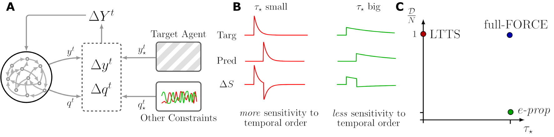
Figure 1: Framework schematics. (A) Graphical depiction of a general Behavioural Cloning task. An agent (here a recurrent network) observes the current state-action pair of a target agent and is trained to emulate such behaviour. The model assumes the presence of additional constraints. The total number of independent constraints $D$ defines the rank of the error propagation matrix. (B) Schematics of difference $\tau_{\star}$, the spikes filtering timescales. A larger $\tau_{\star}$ is more tolerant on precise spike timing. (C) Schematics of our generalized framework. Changing the $D$ and $\tau_{\star}$ parameters, it is possible to derive different learning algorithms.

3.1.2 Target-based approach

The possibility to broadcast specific local errors in biological networks has been debated for a long time [32, 23]. On the other hand, the propagation of a target appears to be more coherent with biological observations [18, 26, 35, 20]. For this reason we propose an alternative formulations allowing to evaluate target rather than errors [25, 23]. This can be easily done by writing the target output as:

$$Y_{i}^{\star\ t}={\mathsf{R}}_{ik}r_{k}^{\star\ t}.$$ (10)

Where $r_{k}^{\star\ t}$ is the target activity of the recurrent network. We observe that if the matrix $\mathsf{R}_{ik}$ is full rank, the internal target can be easily uniquely defined, otherwise it exists a degeneracy in its choice. Substituting this expression in eq. (9) we obtain

$$\Delta w_{ij}=\eta\sum_{t}\left[\sum_{k}\left({\mathsf{R}}^{\top}{\mathsf{R}}\right)_{ik}\left(r_{k}^{\star t+1}-s_{k}^{t+1}\right)\right]p_{i}^{t}e_{j}^{t},$$ (11)

By inspection, we notice the occurrence of a novel matrix ${\mathsf{D}}={\mathsf{R}}^{\top}{\mathsf{R}}$ which acts recurrently on the network, ${\mathsf{D}}\in\mathbb{R}^{N\times N}$. If one now forgets the origin of this novel matrix, the previous relation can be rewritten in terms of a general square matrix ${\mathsf{D}}\in\mathbb{R}^{N\times N}$:

$$\Delta w_{ij}=\eta\sum_{t}\left[\sum_{k}{\mathsf{D}}_{ik}\left(r_{k}^{\star t+1}-s_{k}^{t+1}\right)\right]p_{i}^{t}e_{j}^{t}.$$ (12)

The two core new terms are the $r_{i}^{\star t}$ and the matrix ${\mathsf{D}}$. The first induces the problem of selecting the optimal network activity, which is tautologically a re-statement of the learning problem. The second term, the matrix ${\mathsf{D}}$ defines the dynamics in the space of the internal network activities $s_{k}^{t}$ during learning. This formulation results similar to the full-FORCE algorithm [10], which is target-based, but does not impose a specific pattern of spikes for the internal solution.

3.1.3 Spike coding approximation

We want now to replace the target internal activity $r_{i}^{\star\ t}$ with a target sequence of spikes $s_{i}^{\star\ t}$, in order to approximate the $Y_{i}^{\star\ t}$ as:

$$Y_{i}^{\star\ t}\simeq{\mathsf{R}}_{ik}\bar{s}_{k}^{\star\ t}.$$ (13)

We stress here the fact that, due to the spikes quantization, the equality cannot be strictly achieved, and eq. (13) is an approximation. One can simply consider ${s}^{\star t}$ to be the solution of the optimization problem $s_{i}^{\star t}=\mathrm{argmin}_{s_{i}^{\star t}}\sum_{kt}|y_{k}^{\star t}-\sum_{i}{\mathsf{B}}_{ki}\bar{s}_{i}^{\star t}|$. The optimal encoding for a continuous trajectory through a pattern of spikes has been broadly discussed in [5]. However, the pattern ${s}^{\star t}$ might describe an impossible dynamics (for example activity that follows periods of complete network silence). For this reason here we take a different choice. The $s_{i}^{\star t}$ is the pattern of spikes expressed by the untrained network when the target output $Y_{i}^{\star t}$ is randomly projected as an input (similarly to [10, 28]). It has been demonstrated that this choice allows for fast convergence and encodes detailed information about the target output. With these additional considerations, we can now rewrite our expression for the weight update in terms of the network activity:

$$\Delta w_{ij}=\eta\sum_{t}\left[\sum_{k}{\mathsf{D}}_{ik}\left(\bar{s}_{k}^{\star t+1}-\bar{s}_{k}^{t+1}\right)\right]p_{i}^{t}e_{j}^{t}.$$ (14)

In this way a specific pattern of spikes is directly suggested to the network as the internal solution of the task. We observe that when ${\mathsf{R}}$ is random and full rank, ${\mathsf{D}}$ it is almost diagonal and the training of recurrent weights reduces to learning a specific pattern of spikes [31, 16, 12, 4, 7]. In this limit the model LTTS [28] is recovered (see Fig.1C), with the only difference of the presence of the pseudo-derivative. We interpret the parameter $\tau_{\star}$ (the time scale of the spike filtering, see eq. (4)) as the tolerance to spike timing. In Fig.1B we show in a sketch that, for the same spike displacement between the internal and the target activity, the error is higher when the $\tau_{\star}$ is lower.

3.2 Numerical Results

3.2.1 Dimensionality of the solution space

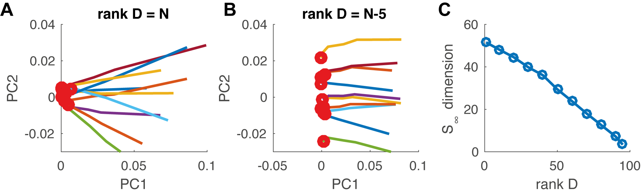
Figure 2: Error propagation and dimensionality of the internal solution. (A). Dynamics along training epochs of the $\Delta S_{i}=\sum_{t}\left|s_{i}^{\star\ t}-s_{i}^{t}\right|$ in the first two principal components for different repetition of the training with variable initial conditions. The error propagation matrix has maximum rank ($\mathcal{D}=N$, target-based limit). (B). Same as in (A), but with an error propagation matrix with rank $\mathcal{D}=N-5$. (C). Dimensionality of the solution space $\mathcal{S}_{\infty}$ as a function of the rank $\mathcal{D}$ of the error propagation matrix.

The learning formulation of eq. (14) offers a major insights on the role played by the feedback matrix ${\mathsf{D}}_{ik}$. Consider the learning problem (with fixed input and target output) where the synaptic matrix $w_{ij}$ is refined to minimize the output error (by converging to the proper internal dynamics). The learning dynamics can be easily pictured as a trajectory where a single point is a complete history of the network activity ${s}_{n}=\left\{s_{i}^{t}:i=1,...N;t=1,...T\right\}$. Upon initialization, a network is located at a point ${s}_{0}$ marking its untrained spontaneous dynamics. The following point ${s}_{1}$ is the activity produced by the network after applying the learning rule defined in eq. (14), and so on. By inspecting eq. (14) one notes that a sufficient condition for halting the learning is $|\sum_{i}{\mathsf{D}}_{hi}\left(\bar{s}_{i}^{\star\ t}-\bar{s_{i}}^{t}\right)|<\epsilon$, where $\epsilon$ is an arbitrary small positive number. If $\epsilon$ is small enough it is possible to write:

$$\sum_{i}{\mathsf{D}}_{hi}\left(\bar{s}_{i}^{\star\ t}-\bar{s_{i}}^{t}\right)\simeq 0.$$ (15)

In the limit of a full-rank ${\mathsf{D}}$ matrix (example: the LTTS limit where ${\mathsf{D}}$ is diagonal) the only solution to eq. (15) is $\bar{{s}}^{t}\simeq\bar{{s}}^{\star t}$ and the learning halts only when target $\bar{{s}}^{\star\ t}$ is cloned. When the rank is lower the solution to eq. (15) is not unique, and the dimensionality of possible solutions is defined by the kernel of the matrix ${\mathsf{D}}$ (the collection of vectors ${\lambda}$ such that ${\mathsf{D}}{\lambda}=0$). We have: $\mathrm{dim}\ \mathrm{Ker}\ {\mathsf{D}}=N-\mathrm{rank}\ {\mathsf{D}}=N-\mathcal{D}$. We run a numerical experiment in order to confirm our theoretical predictions. We used equation (14) to store and recall a 3D continuous trajectory $y_{k}^{\star\ t}$ ($k=1,..3$, $t=1,..T$, $T=100$) in a network of $N=100$ neurons. $y_{k}^{\star\ t}$ is a temporal pattern composed of $3$ independent continuous signals. Each target signal is specified as the superposition of the four frequencies $f\in\left\{1,2,3,5\right\}$ Hz with uniformly extracted random amplitude $A\in\left[0.5,2.0\right]$ and phase $\phi\in\left[0,2\pi\right]$. We repeated the experiment for different values of the rank $\mathcal{D}$. The matrix ${\mathsf{R}}_{ik}=\frac{\delta_{ik}}{\sqrt{\mathcal{D}}}$, $i=1,...N$, $k=1,...\mathcal{D}$, where $\delta_{ik}$ is the Kronecker delta (the analysis for the case ${\mathsf{R}}_{ik}$ random provides analogous results and is reported in the supplemental material). When the rank is $N$, different replicas of the learning (different initializations of recurrent weights) converge almost to the same internal dynamics $s_{i}^{t}$. This is reported in Fig.2A where a single trajectory represents the first 2 principal components (PC) of the vector $\sum_{t}|s_{i}^{\star\ t}-s_{i}^{t}|$. The convergence to the point $(0,0)$ represents the convergence of the dynamics to $s_{i}^{\star\ t}$. When the rank is lower ($\mathcal{D}=N-5$, see Fig.2B) different realizations of the learning converge to different points, distributed on an line in the PC space. This can be generalized by investigating the dimension of the convergence space as a function of the rank. The dimension of the vector $s_{i}^{\star\ t}-s_{i}^{t}$ evaluated in a the trained network is estimated as $d=\frac{1}{\sum_{k}\lambda_{k}^{2}}$, where $\lambda_{k}$ are the principal component variances normalized to one ($\sum_{k}\lambda_{k}$ = 1). We found a monotonic relation between the dimension of the convergence space and the rank (see Fig.2C, more information on the PC analysis and the estimation of the dimensionality in the supplemental material). This observation confirms that when the rank is very high, the solution is strongly constrained, while when the rank becomes lower, the internal solution is free to move in a subspace of possible solutions. We suggest that this measure can be used in biological data to estimate the dimensionality of the learning constraints in biological neural network from the dimensionality of the solution space.

3.2.2 Tolerance to spike timing

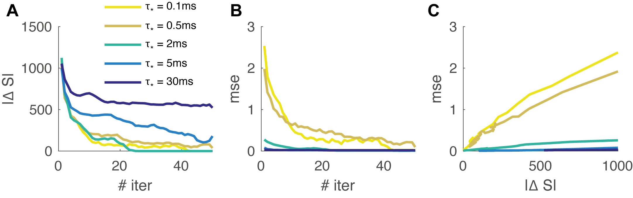
Figure 3: Target-based learning for different time-scales. (A). Color-coded the error on the spike sequence $\Delta S=\sum_{it}|s_{i}^{\star\ t}-s_{i}^{t}|$ as a function of the number of iterations for different $\tau_{\star}$. (B). Color-coded the $\mathrm{mse}=\sum_{kt}(y_{k}^{\star\ t}-y_{k}^{t})^{2}$ as a function of the number of iterations for different $\tau_{\star}$. (C). Scatter plot of $\mathrm{mse}$ vs $\Delta S$ for different values of $\tau_{\star}$.

As we discussed above the $\tau_{\star}$ can be interpreted as the tolerance to precise spike timing. To investigate the role of this parameter, we considered the same store and recall task of a 3D trajectory described in the previous section ($N=100$, $T=100$). We set the maximum rank ($\mathcal{D}=N$) for this experiment. In Fig.3A we report the spike error $\Delta S=\sum_{it}\left|s_{i}^{\star\ t}-s_{i}^{t}\right|$ as a function of the iteration number for different values of the parameter $\tau_{\star}$. Only for the lower values of $\tau_{\star}$ the algorithm converges exactly to the spike pattern $s_{i}^{\star\ t}$. In Fig.3B we report the $\mathrm{mse}=\sum_{kt}(y_{k}^{\star\ t}-y_{k}^{t})^{2}$ as a function of the iteration numbers and the parameter $\tau_{\star}$. In Fig.3C we show the $\mathrm{mse}$ as a function of $\Delta S$ for different values of $\tau_{\star}$. Lower $\tau_{\star}$ values are characterized by a higher slope meaning that a change in the spike pattern expressed by the network strongly affects the error on the output $y_{k}^{t}$. This suggests a low tolerance to precise spike timing in the generated output when the parameter $\tau_{\star}$ is low. The consequence of this effect in a behavioral task is investigated below (section 2D Bipedal Walker).

3.3 Application to closed-loop tasks

3.3.1 Button-and-food task

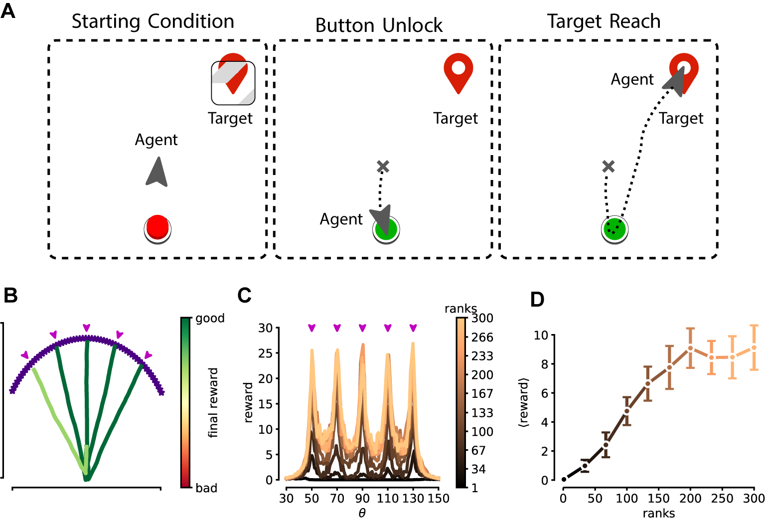
Figure 4: Button-and-food task. (A) Sketch of the task. An agent start at the center of the environment domain (left) and is asked to reach a target. The target is initially "locked". The agent must unlock the target by pushing a button (middle) placed behind and then reach for the target (right). (B) Example trajectories produced by a trained agent for different target locations. Purple arrows depict the observed expert behaviours. (C) Final reward obtained by a trained agents as a function of the target position (measured by the angle $\theta$ with a fixed radius of $r=0.7$ as measured from the agent starting position). Continuous lines are average values, while error bars are standard deviation for $10$ repetitions. Colors codes for different ranks in the error propagation matrix. (D) Average reward as a function of the rank.

To investigate the effect of the rank $\mathcal{D}$ of feedback matrix, we design a button-and-food task (see Fig.4A for a graphical representation), which requires for a precise trajectory and to retain the memory of the past states. In this task, the agent starts at the center of the scene, which features also a button and an initially locked target (the food). The agent task is to first push the button so to unlock the food and then reach for it. We stress that to change its spatial target from the button to the food, the agents has to remember that it already pressed the button (the button state is not provided as an input to the network during the task). In our experiment we kept the position of the button (expressed in polar coordinates) fixed at $r_{\mathrm{btn}}=0.2$, $\theta_{\mathrm{btn}}=-90^{\circ}$ for all conditions, while food position had $r_{\mathrm{targ}}=0.7$ and variable $\theta_{\mathrm{targ}}\in\left[30^{\circ},150^{\circ}\right]$. The agent learns via observations of a collection of experts behaviours, which we indicate via the food positions $\left\{\theta_{\mathrm{targ}}^{\star}\right\}$. The expert behavior is a trajectory which reaches the button and then the food in straight lines ($T=80$). The network receives as input ( $I=80$ input units) the vertical and horizontal differences of both the button’s and food’s positions with respect to agent location ($\Delta^{t}=\{\Delta x_{b}^{t},\Delta y_{b}^{t},\Delta x_{f}^{t},\Delta y_{f}^{t}\}$ respectively). These quantities are encoded through a set of tuning curves. Each of the $\Delta_{i}$ values are encoded by 20 input units with different Gaussian activation functions. Agent output is the velocity vector $v_{x,y}$ ($O=2$ output units). We used $\eta=\eta_{\mathrm{RO}}=0.01$ (with Adam optimizer), moreover $\tau_{\mathrm{RO}}=10\mathrm{ms}$. Agent performances are measured with the inverse of final agent-food distance for unlocked food $r_{\mathrm{unlocked}}=d\left(p_{\mathrm{agent}},p_{\mathrm{target}}\right)^{-1}$, and kept fixed at $r_{\mathrm{locked}}=1/d_{\mathrm{max}}$ (with $d_{\mathrm{max}}=5$) for the locked condition. We repeated training for different values of the rank of the feedback matrix ${\mathsf{D}}$, computed from ${\mathsf{R}}_{ik}=\frac{\delta_{ik}}{\sqrt{\mathcal{D}}}$ (with $\delta_{ik}$ the Kronecker delta, the analysis for the case ${\mathsf{R}}_{ik}$ random provides analogous results and is reported in the supplemental material), in a network of $N=300$ neurons, and compared the overall performances (more information in the supplemental material). Results for such experiment are reported in Fig.4B-C. Fig.4B, we report the agent training trajectories, color-coded for the final reward. Indeed all the training conditions ($\theta^{\star}_{\mathrm{targ}}\in\left\{50,70,90,110,130\right\}$) show good convergence. In Fig.5C the final reward is reported as a function of the target angle $\theta_{\mathrm{targ}}$ for different ranks (purple arrows indicate the training conditions). As expected, the reward is maximum concurrently to the training condition. Moreover, it can be readily seen how high-rank feedback structures allows for superior performances for this task.

3.3.2 2D Bipedal Walker

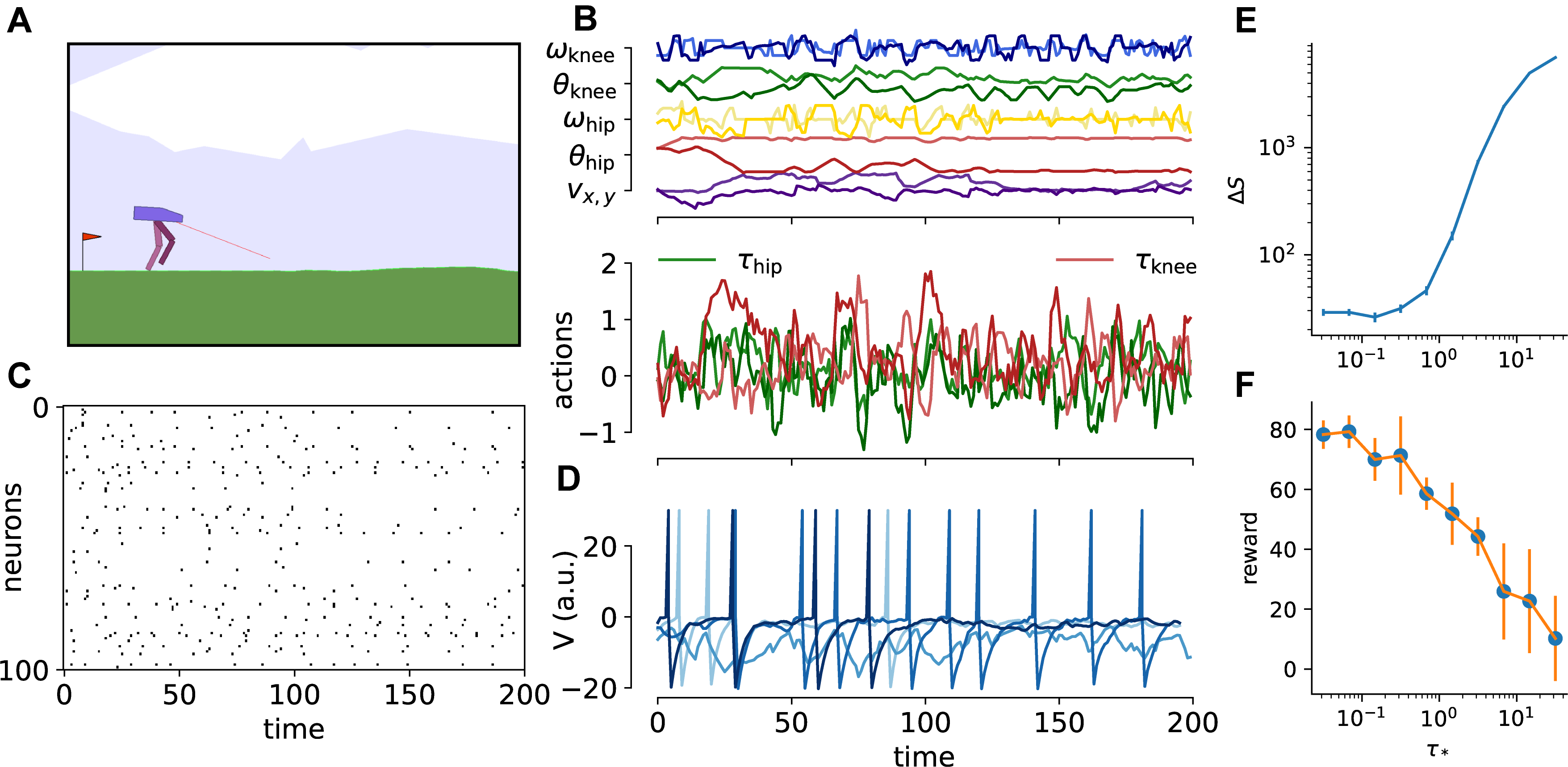
Figure 5: 2D Bipedal Walker. (A). Representation of the 2D Bipedal Walker environment. The task is to successfully control the bipedal locomotion of the agent, reward is measured as the travelled distance across the horizontal direction. (B) (Top) Temporal dynamics of the core input state variable. $v_{x,y}$ is the velocity direction in the bi-dimensional plane. $\omega_{\mathrm{knee},\mathrm{hip}}$ are the angular velocity of the two leg joints, while $\theta_{\mathrm{knee},\mathrm{hip}}$ are the corresponding angles. Each angular variable has two components which corresponds to the two legs of the agent, which are depicted via different shades of the same color. (Bottom) Temporal dynamics of the action vector. The network controls the agent via the torque $\tau_{\mathrm{hip},\mathrm{knee}}$ that is applied to the two legs. Controls for left and right legs are depicted via different shades of the same color. (C). Rasterplot of the activity of a random sample of $100$ neurons across $200$ time unit of a task episode. (D). Temporal dynamics of the membrane potential of four example units. (E). Spike error $\Delta S$ as a function of the $\tau_{\star}$. (F). Average reward as a function of the $\tau_{\star}$.

We benchmarked our behavioral cloning learning protocol on the standard task the 2D Bipedal Walker, provided through the OpenAI gym (https://gym.openai.com [6], MIT License). The environment and the task are sketched in Fig.5A: a bipedal agent has to learn to walk and to travel as long a distance as possible. The expert behavior is obtained by training a standard feed-forward network with PPO (proximal policy approximation [34], in particular we used the code provided in [1], MIT License). The sequence of states-actions is collected in the vectors ${y}^{\star\ t}_{k}$, $k=1,...\,O$, ${x}^{\star\ t}_{h}$, $h=1,...I$, $t=1,...T$, with $T=400$, $O=4$, $I=15$ (see In Fig.5C for an example of the states-actions trajectories). The average reward performed by the expert is $\langle r\rangle_{exp}\simeq 180$ while a random agent achieves $\langle r\rangle_{rnd}\simeq-120$. We performed behavioral cloning by using the learning rule in eq. (14) in a network of $N=500$ neurons. We chose the maximum rank ($\mathcal{D}=N$) and evaluate the performances for different values of $\tau_{\star}$ (more information in the supplemental material). In Fig.5B-C it is report the rastergram for $100$ random neurons and the dynamics of the membrane potential for $3$ random neurons during a task episode. For each value of $\tau_{\star}$ we performed $10$ independent realizations of the experiment. For each realization the $s_{i}^{\star\ t}$ is computed, and the recurrent weights are trained by using eq. (14). The optimization is performed using gradient ascent and a learning rate $\eta=1.0$. In Fig.5D we report the spike error $\Delta S=\sum_{it}\left|s_{i}^{\star\ t}-s_{i}^{t}\right|$ at the end of the training. The internal dynamics $s_{i}^{t}$ almost perfectly reproduces the target pattern of spikes $s_{i}^{\star\ t}$ for $\tau_{\star}<0.5\mathrm{ms}$, while the error increases for larger values. The readout time-scale is fixed to $\tau_{\mathrm{RO}}=5\mathrm{ms}$ while the readout weights are initialized to zero and the learning rate is set to $\eta_{\mathrm{RO}}=0.01$. Every $75$ training iterations of the readout we test the network and evaluate the average reward $\langle r\rangle$ over $50$ repetitions of the task. We then evaluate the average over the $10$ realizations of the maximum $\langle r\rangle$ obtained for each realization. In Fig.5F it is reported the average of the maximum reward as a function of $\tau_{\star}$. The decreasing monotonic trend suggests that learning with specific pattern of spikes ($\tau_{\star}\rightarrow 0$) enables for optimal performances in this walking task. We stress that in this experiment we used a clumped version of the learning rule. In other words we substituted $s_{i}^{\star\ t}$ to $s_{i}^{t}$ in the evaluation of $\frac{\partial v_{i}}{\partial w_{ij}}$ in eq.(7). This choice, which is only possible when the maximum rank is considered ($\mathcal{D}=N$), allows for faster convergence and better performances. The results for the non-clumped version of the learning rule are reported in the supplemental material.

4 Discussion

In this work, we introduced a general framework for supervised learning in recurrent spiking networks, with two main parameters, the rank of the feedback error propagation $\mathcal{D}$ and the tolerance to precise spike timing $\tau_{\star}$ (see Fig.1C). We argue that many proposed learning rules can be seen as specific cases of our general framework (e-prop, LTTS, full-FORCE). In particular, the generalization on the rank of the feedback matrix allowed us to understand the target-based approaches as emerging from error-based ones when the number of independent constraints is high. Moreover, we understood that different $\mathcal{D}$ values lead to different dimensionality of the solution space. If we see the learning as a trajectory in the space of internal dynamics, when the rank $\mathcal{D}$ is maximum, every training converges to the same point in this space. On the other hand, when the $\mathcal{D}$ is lower, the solution is not unique, and the possible solutions are distributed in a subspace whose dimensionality is inversely proportional to the rank of the feedback matrix. We suggest that this finding can be used to produce experimental observable to deduce the actual structure of error propagation in the different regions of the brain. On a technological level, our approach offers a strategy to clone on a (spiking) chip an expert behavior either previously learned via standard reinforcement learning algorithms or acquired from a human agent. Our formalism can be directly applied to train an agent to solve closed-loop tasks through a behavioral cloning approach. This allowed solving tasks that are relevant in the reinforcement learning framework by using a recurrent spiking network, a problem that has been faced successfully only by a very small number of studies [2]. Moreover, our general framework, encompassing different learning formulations, allowed us to investigate what learning method is optimal to solve a specific task. We demonstrated that a high number of constraints can be exploited to obtain better performances in a task in which it was required to retain a memory of the internal state for a long time (the state of the button in the button-and-food task). On the other hand, we found that a typical motor task (the 2D Bipedal Walker) strongly benefits from precise timing coding, which is probably due to the necessity to master fine movement controls to achieve optimal performances. In this case, a high rank in the error propagation matrix is not really relevant. From the biological point of view, we conjecture that different brain areas might be located in different positions in the plane presented in Fig.1C.

4.1 Limitations of the study

We chose relevant but very simple tasks in order to test the performances of our model and understand its properties. However, it is very important to demonstrate if this approach can be successfully applied to more complex tasks, e.g. requiring both long-term memory and fine motor skills. It would be of interest to measure what are the optimal values for both the rank of feedback matrix and $\tau_{\star}$in a more demanding task. Finally, we suggested that our framework allows for inferring the error propagation structure. However, our measure requires knowing the target internal dynamics which is not available in experimental recordings. We plan to develop a variant of this measure that doesn’t require such an observable. Moreover, we observe that the measure we proposed is indirect since it is necessary to estimate the dimensionality of the solution space first and then deduce the dimensionality of the learning constraints. Future development of the theory might be to formulate a method that directly infers from the data the laws of the dynamics in the solution space induced by learning.

References

- [1] Nikhil Barhate “Minimal PyTorch Implementation of Proximal Policy Optimization” MIT Licence In GitHub repository GitHub, https://github.com/nikhilbarhate99/PPO-PyTorch, 2021
- [2] Guillaume Bellec et al. “A solution to the learning dilemma for recurrent networks of spiking neurons” In Nature communications 11.1 Nature Publishing Group, 2020, pp. 1–15
- [3] Guillaume Bellec et al. “Long short-term memory and learning-to-learn in networks of spiking neurons” In arXiv preprint arXiv:1803.09574, 2018
- [4] Johanni Brea, Walter Senn and Jean-Pascal Pfister “Matching recall and storage in sequence learning with spiking neural networks” In Journal of neuroscience 33.23 Soc Neuroscience, 2013, pp. 9565–9575
- [5] Wieland Brendel et al. “Learning to represent signals spike by spike” In PLoS computational biology 16.3 Public Library of Science San Francisco, CA USA, 2020, pp. e1007692
- [6] Greg Brockman et al. “OpenAI Gym”, 2016 eprint: arXiv:1606.01540
- [7] Cristiano Capone, Guido Gigante and Paolo Del Giudice “Spontaneous activity emerging from an inferred network model captures complex spatio-temporal dynamics of spike data” In Scientific reports 8.1 Nature Publishing Group, 2018, pp. 1–12
- [8] Cristiano Capone, Elena Pastorelli, Bruno Golosio and Pier Stanislao Paolucci “Sleep-like slow oscillations improve visual classification through synaptic homeostasis and memory association in a thalamo-cortical model” In Scientific Reports 9.1 Nature Publishing Group, 2019, pp. 8990
- [9] CE Carr and M Konishi “A circuit for detection of interaural time differences in the brain stem of the barn owl” In Journal of Neuroscience 10.10 Soc Neuroscience, 1990, pp. 3227–3246
- [10] Brian DePasquale, Christopher J Cueva, Kanaka Rajan and LF Abbott “full-FORCE: A target-based method for training recurrent networks” In PloS one 13.2 Public Library of Science, 2018, pp. e0191527
- [11] Peter Diehl and Matthew Cook “Unsupervised learning of digit recognition using spike-timing-dependent plasticity” In Frontiers in Computational Neuroscience 9, 2015, pp. 99 DOI: 10.3389/fncom.2015.00099
- [12] Brian Gardner and André Grüning “Supervised learning in spiking neural networks for precise temporal encoding” In PloS one 11.8 Public Library of Science, 2016, pp. e0161335
- [13] Tim Gollisch and Markus Meister “Rapid neural coding in the retina with relative spike latencies” In science 319.5866 American Association for the Advancement of Science, 2008, pp. 1108–1111
- [14] Bruno Golosio et al. “Thalamo-cortical spiking model of incremental learning combining perception, context and NREM-sleep” In PLoS Computational Biology 17.6 Public Library of Science San Francisco, CA USA, 2021, pp. e1009045
- [15] Alessandro Ingrosso and LF Abbott “Training dynamically balanced excitatory-inhibitory networks” In PloS one 14.8 Public Library of Science San Francisco, CA USA, 2019, pp. e0220547
- [16] Danilo Jimenez Rezende and Wulfram Gerstner “Stochastic variational learning in recurrent spiking networks” In Frontiers in Computational Neuroscience 8, 2014, pp. 38 DOI: 10.3389/fncom.2014.00038
- [17] Roland S Johansson and Ingvars Birznieks “First spikes in ensembles of human tactile afferents code complex spatial fingertip events” In Nature neuroscience 7.2 Nature Publishing Group, 2004, pp. 170
- [18] Eric I Knudsen “Supervised learning in the brain” In Journal of Neuroscience 14.7 Soc Neuroscience, 1994, pp. 3985–3997
- [19] Elena Kreutzer, Mihai A Petrovici and Walter Senn “Natural gradient learning for spiking neurons” In Proceedings of the Neuro-inspired Computational Elements Workshop, 2020, pp. 1–3
- [20] Matthew Evan Larkum “A cellular mechanism for cortical associations: an organizing principle for the cerebral cortex” In Trends in Neurosciences 36, 2013, pp. 141–151
- [21] Dong-Hyun Lee, Saizheng Zhang, Asja Fischer and Yoshua Bengio “Difference target propagation” In Joint european conference on machine learning and knowledge discovery in databases, 2015, pp. 498–515 Springer
- [22] Timothy P Lillicrap, Daniel Cownden, Douglas B Tweed and Colin J Akerman “Random synaptic feedback weights support error backpropagation for deep learning” In Nature communications 7.1 Nature Publishing Group, 2016, pp. 1–10
- [23] Nikolay Manchev and Michael W Spratling “Target Propagation in Recurrent Neural Networks.” In Journal of Machine Learning Research 21.7, 2020, pp. 1–33
- [24] Raoul-Martin Memmesheimer, Ran Rubin, Bence P Ölveczky and Haim Sompolinsky “Learning precisely timed spikes” In Neuron 82.4 Elsevier, 2014, pp. 925–938
- [25] Alexander Meulemans et al. “A theoretical framework for target propagation” In arXiv preprint arXiv:2006.14331, 2020
- [26] R Chris Miall and Daniel M Wolpert “Forward models for physiological motor control” In Neural networks 9.8 Elsevier, 1996, pp. 1265–1279
- [27] Milad Mozafari et al. “Bio-inspired digit recognition using reward-modulated spike-timing-dependent plasticity in deep convolutional networks” In Pattern Recognition 94 Elsevier, 2019, pp. 87–95
- [28] Paolo Muratore, Cristiano Capone and Pier Stanislao Paolucci “Target spike patterns enable efficient and biologically plausible learning for complex temporal tasks” In PloS one 16.2 Public Library of Science San Francisco, CA USA, 2021, pp. e0247014
- [29] Wilten Nicola and Claudia Clopath “Supervised learning in spiking neural networks with FORCE training” In Nature communications 8.1 Nature Publishing Group, 2017, pp. 2208
- [30] Stefano Panzeri et al. “The role of spike timing in the coding of stimulus location in rat somatosensory cortex” In Neuron 29.3 Elsevier, 2001, pp. 769–777
- [31] Jean-Pascal Pfister, Taro Toyoizumi, David Barber and Wulfram Gerstner “Optimal spike-timing-dependent plasticity for precise action potential firing in supervised learning” In Neural computation 18.6 MIT Press, 2006, pp. 1318–1348
- [32] Pieter R Roelfsema and Arjen van Ooyen “Attention-gated reinforcement learning of internal representations for classification” In Neural computation 17.10 MIT Press, 2005, pp. 2176–2214
- [33] João Sacramento, Rui Ponte Costa, Yoshua Bengio and Walter Senn “Dendritic cortical microcircuits approximate the backpropagation algorithm” In Advances in Neural Information Processing Systems 31 Curran Associates, Inc., 2018, pp. 8721–8732
- [34] John Schulman et al. “Proximal policy optimization algorithms” In arXiv preprint arXiv:1707.06347, 2017
- [35] MW Spratling “Cortical region interactions and the functional role of apical dendrites” In Behavioral and cognitive neuroscience reviews 1.3 Sage Publications Sage CA: Thousand Oaks, CA, 2002, pp. 219–228
- [36] Manuel Traub, Robert Legenstein and Sebastian Otte “Many-Joint Robot Arm Control with Recurrent Spiking Neural Networks” In arXiv preprint arXiv:2104.04064, 2021
- [37] Robert Urbanczik and Walter Senn “Learning by the dendritic prediction of somatic spiking” In Neuron 81.3 Elsevier, 2014, pp. 521–528
- [38] Friedemann Zenke and Surya Ganguli “Superspike: Supervised learning in multilayer spiking neural networks” In Neural computation 30.6 MIT Press, 2018, pp. 1514–1541