The Rapid ASKAP Continuum Survey Paper II: First Stokes I Source Catalogue Data Release

Abstract

The Rapid ASKAP Continuum Survey (RACS) is the first large sky survey using the Australian Square Kilometre Array Pathfinder (ASKAP), covering the sky south of +41^∘ declination. With ASKAP’s large, instantaneous field of view, $\sim 31$ deg², RACS observed the entire sky at a central frequency of 887.5 MHz using 903 individual pointings with 15 minute observations. This has resulted in the deepest radio survey of the full Southern sky to date at these frequencies. In this paper, we present the first Stokes I catalogue derived from the RACS survey. This catalogue was assembled from 799 tiles that could be convolved to a common resolution of 25^′′, covering a large contiguous region in the declination range $\delta=-$80^∘ to +30^∘. The catalogue provides an important tool for both the preparation of future ASKAP surveys and for scientific research. It consists of $\sim$2.1 million sources and excludes the $|b|<5$^∘ region around the Galactic plane. This provides a first extragalactic catalogue with ASKAP covering the majority of the sky ($\delta<+30$^∘). We describe the methods to obtain this catalogue from the initial RACS observations and discuss the verification of the data, to highlight its quality. Using simulations, we find this catalogue detects 95% of point sources at an integrated flux density of $\sim$5 mJy. Assuming a typical sky source distribution model, this suggests an overall 95% point source completeness at an integrated flux density $\sim$3 mJy. The catalogue will be available through the CSIRO ASKAP Science Data Archive (CASDA).

1 INTRODUCTION

Radio surveys provide unique views into the Galactic and extragalactic skies. At the frequency of the Rapid ASKAP Continuum Survey (RACS, at 887.5 MHz; McConnell et al., 2020), and more generally below a few GHz, radio emission is dominated by synchrotron radiation; the emission from relativistic electrons spiralling within magnetic fields (Condon, 1992). This traces two main extragalactic populations: Active Galactic Nuclei (AGN) and Star Forming Galaxies (SFGs). For SFGs, it provides a method of obtaining unbiased star formation rates (SFR; e.g. Bell, 2003; Garn et al., 2009; Davies et al., 2017; Gürkan et al., 2018), as radio emission is un-attenuated by dust. Observing synchrotron emission from AGN is important for understanding galaxy evolution, as their feedback is thought to limit the size to which galaxies can grow (see e.g. Bower et al., 2006; Fabian, 2012; Harrison, 2017). Within the Galaxy, radio emission is often observed from supernova remnants (see e.g. Whiteoak & Green, 1996; Anderson et al., 2017), as Galactic synchrotron emission within the Galactic plane (see e.g. Haslam et al., 1982; Green et al., 1999; Murphy et al., 2007; Wang et al., 2018) as well as from transient and variable sources (see e.g. Thyagarajan et al., 2011; Bhandari et al., 2018). This variety of objects motivates radio surveys for advancing our understanding of the Universe.

For catalogues of extragalactic radio sources, it is important to have both large area as well as deep observations. Deeper, smaller area surveys provide observations of fainter radio populations (e.g. radio quiet quasars and SFGs, see e.g. Wilman et al., 2008; Padovani et al., 2015; Smolčić et al., 2017b) and allow galaxy evolution to be investigated to earlier times in the age of the Universe. Large area surveys, on the other hand, allow extreme and rare AGN to be observed as well as large samples of resolved nearby SFGs. They are also crucial in providing information for radio sky models. Moreover, observations at multiple epochs of large sky areas are useful for detecting transient or variable sources (see e.g. Thyagarajan et al., 2011; Mooley et al., 2016; Nyland et al., 2020).

At $\sim$1 GHz, radio surveys which have observed large regions of the southern skies ($\delta<0$^∘) have been dominated by the combination of Sydney University Molonglo Sky Survey (SUMSS; Mauch et al., 2003), the Molongolo Galactic Plane Survey (MGPS; Green et al., 1999) and the updated MGPS-2 survey (Murphy et al., 2007) as well as the NRAO VLA Sky Survey (NVSS; Condon et al., 1998), complemented in the smaller overlap regions by Faint Images of the Radio Sky at Twenty-Centimeters (FIRST; Becker et al., 1995; Helfand et al., 2015). SUMSS surveyed the southern sky up to a northern-most $\delta=-$30^∘ (excluding the Galactic plane $|b|<10$^∘) at 843 MHz with 45^′′/$\sin|\delta|$ resolution at a typical sensitivity of $\sim$1 mJy/beam. NVSS, on the other hand, is a northern sky survey which observed to a southern-most $\delta=-$40^∘ at 1.4 GHz, observing with a constant 45^′′ resolution at a typical sensitivity of $\sim$0.5 mJy/beam. FIRST also observed at 1.4 GHz with the VLA to a deeper sensitivity of $\sim$0.15 mJy/beam, at 5^′′ resolution around the north and south Galactic caps. However, FIRST does not probe a large fraction of the southern skies and has limited sensitivity to extended emission.

At lower frequencies, the Galactic and Extra-Galactic All-sky MWA Survey (GLEAM; Hurley-Walker et al., 2017) and TIFR GMRT Sky Survey Alternate Data Release (TGSS-ADR; Intema et al., 2017) provided observations of large regions of the southern sky. GLEAM observed south of $\delta$ = +30^∘ at $\sim$2^′ resolution, reaching a root mean square (rms) sensitivity of 6$-$10 mJy/beam in the frequency range 70$-$230 MHz. TGSS-ADR observed the entire sky north of $\delta=-$53^∘ at higher resolution, $\sim$25^′′, to an rms sensitivity of approximately 3.5 mJy/beam at 150 MHz. At higher frequencies, the Australia Telescope Compact Array (ATCA) has conducted surveys of the southern radio sky, including the Australia Telescope 20 GHz Survey (AT20G; Murphy et al., 2010), with approximately 10^′′ resolution, yielding a catalogue to an integrated flux density limit of 40 mJy (for $\delta<0$^∘). All these large area surveys are crucial to improving statistics on galaxy numbers, finding rare objects, as well as observing nearby radio sources and resolved star forming galaxies. Moreover, the combination of low, mid and high radio frequency radio surveys are important for spectral modelling of sources (see e.g. Clemens et al., 2008; Galvin et al., 2018).

In order to observe such large areas it is advantageous to have an instrument with a large field of view. The Australian SKA Pathfinder (ASKAP; Johnston et al., 2008; Hotan et al., 2014; Hotan et al., 2021) is one such facility able to easily conduct large sky surveys. It uses phased array feeds (PAFs), which provide an instantaneous field of view of 31 deg². The first large sky survey with ASKAP is the Rapid ASKAP Continuum Survey (RACS) and has been described in detail in Paper I (McConnell et al., 2020). RACS used 15 minute observations to image the sky south of $\delta=+$41^∘ using 903 tiles with typical sensitivities of 0.25$-$0.3 mJy/beam. Each tile is defined as the mosaic of the individual 36 beams which are simultaneously observed using the PAF technology. This survey therefore provides the best knowledge of radio sources at gigahertz frequencies in the southern hemisphere to date. In the future, the Evolutionary Map of the Universe (EMU; Norris et al., 2011; Norris et al., 2021) will provide a deeper map of the southern sky to $\sim 20\mu$Jy/beam rms, but this will require a significant increase in observation time.

In this paper, we provide the first release of the RACS Stokes I source catalogue. The layout of this paper is as follows. Firstly, we present an overview of RACS in Section 2 and describe the observations used for this first data release. Next, we describe the cataloguing process in Section 3 and the final catalogue in Section 4. We then discuss comparisons to previous surveys in Section 5 before discussing the completeness in Section 6. In Section 7, we present the source counts, both raw and completeness-corrected, for this survey before drawing conclusions in Section 8.

2 Rapid ASKAP Continuum Survey

A detailed description of the RACS tiling and observation strategy can be found in Paper I (McConnell et al., 2020). The majority of RACS observations were initially taken over the course of 12 days during April and May 2019. Subsequently, further re-observations of selected fields were taken in August 2019 and between March-June 2020. The latter re-observations were designed to reduce the PSF variation amongst the 36 beams within each individual tile. Each observation lasted 15 minutes in duration and a calibrator observation (of PKS B1934$-$638) of 200s in duration was typically observed within a day of each observation. These observations covered a 288 MHz bandwidth in the frequency range 744.5$-$1032.5 MHz. In total, 903 tiles were observed to ensure complete coverage of the sky for $\delta\leq$41^∘.

Each observation was processed using ASKAPSoft (see Cornwell et al., 2011; Guzman et al., 2019; Whiting, 2020, and Whiting et al. in prep). This software was specifically designed to take the raw ASKAP visibilities and produce calibrated images of the field, suitable for scientific use. The pipeline parameters used for the RACS survey are described thoroughly in Paper I. A robustness weight of 0.0 (see Briggs, 1995) was used, and short baselines were removed to improve image fidelity for those observations close to the Galactic plane (baselines smaller than 35 m were excluded) or affected by solar interference (baselines smaller than 100 m were excluded). All RACS tile images are on a 2.5^′′ pixel grid and cover $\sim$31 deg². As described in Paper I, after the tile images were formed, a flux correction was applied to the tile to account for differences between the primary beam model applied within ASKAPSoft and the response pattern determined from holography measurements.

Images of each of the 903 tiles have been released publicly on the CSIRO ASKAP Science Data Archive (CASDA, Chapman et al., 2017; Huynh et al., 2020). To construct the first Stokes I catalogue we convolved each tile to a common resolution before mosaicing with neighbouring tiles to reduce sensitivity fluctuations.

2.1 Selected Tiles

A combination of factors affect the resolution of beam images within an individual tile, including: declination, hour angle coverage and the flagging of data within the observations. As ASKAP uses a phased array feed system, each field is constructed from 36 individual beams. The resolution can vary from beam to beam within an individual tile as well as between neighbouring tiles. In order to retain accurate flux scale measurements, it is necessary to ensure these beams and those in neighbouring tiles have the same resolution. This is because radio images are in units of Jy/beam and so varying PSFs in neighbouring images would affect both flux density and shape measurements of sources when mosaiced.

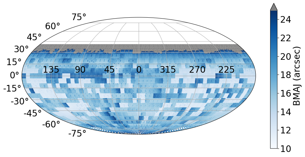
Figure 1: Sky variation of the PSF Major axis (FWHM) for all tiles selected in the database of McConnell et al. (2020) apart from those in Table  1 (see text). This is presented on an equatorial J2000.0 coordinate frame in Mollweide projection.

To determine the fields to include in this first data release it was important to consider the aim of the survey. RACS will provide a model of the observable sky for future ASKAP surveys as well as provide an initial epoch as a benchmark for the search for variable or transient sources. For these purposes it is important to have a resolution as high as possible in order to resolve individual sources, and also to observe a large contiguous region of the sky.

However, it is not possible to simply use those individual beams which have angular resolution better than the desired criterion. This is as the holography corrections, as described in Paper I, requires all 36 beams of a tile to be present. This correction accounts for the differences between the beam models assumed in the ASKAPSoft linear mosaicing function, linmos, compared to that determined by holography measurements. As some beams within tiles can have poor angular resolution compared to other beams within the field, not all of the 903 RACS tiles can be convolved to a desired common resolution.

Using these constraints, we decided upon a common resolution of a circular Gaussian beam with a diameter of 25^′′ (Full Width at Half Maximum, FWHM) for the first catalogue data release. This choice of beam improves on the resolution of surveys such as SUMSS and NVSS by approximately a factor of 2, whilst also ensuring that the included observations cover the majority of the southern sky. The distribution of beam major axes (defined by the FWHM) across the entire RACS survey area released in Paper I is shown in Figure 1. All individual PSF major axes that are above 25^′′ are shown in grey. For tiles in which there have been reobservations, the tile denoted with the column ‘SELECT=1’ in the accompanying database to Paper I was generally chosen. However for a few fields, see Table 1, a different tile to the one selected in Paper I was used. This was because the tile selected could not be convolved to 25^′′, whilst a different observation of the same field could be. This often resulted in these fields having larger rms values, but did result in a continuous observing area. As illustrated in Figure 1, there can be large variations in the PSF major axis across the 903 tiles of the RACS observations.

Tile ID	SBID	Median rms	PSF0 Major	SBID	Median rms	PSF0 Major
	(Tile Used)	(Tile Used)	(Tile Used)	(Paper I)	(Paper I)	(Paper I)
		(mJy/beam)	′′		(mJy/beam)	′′
RACS_0000+18A	13780	0.70	16.7	8572	0.34	22.8
RACS_0259-76A	13715	0.54	19.6	9510	0.27	24.7
RACS_0354-71A	12534	0.26	19.7	8680	0.22	23.4
RACS_1237+12A	13586	1.03	17.2	10469	1.00	17.9
RACS_1710+06A	13761	0.84	14.1	8580	0.37	25.9
RACS_2215+18A	13707	0.63	16.9	8578	0.31	21.1

Table 1: Table listing the six tiles for which this work used a different observation than the ‘best’ observation in Paper I. For each tile we give scheduling block ID (SBID), median rms and PSF major axis of the reference beam.

Figure 2 shows the coverage for the first Stokes I catalogue release area across the sky compared to all of the RACS observations. The region for this first catalogue release (blue in Figure 2) covers the majority of the southern sky with $\delta=-$80^∘ to +30^∘and compromises 799 fields (or tiles).

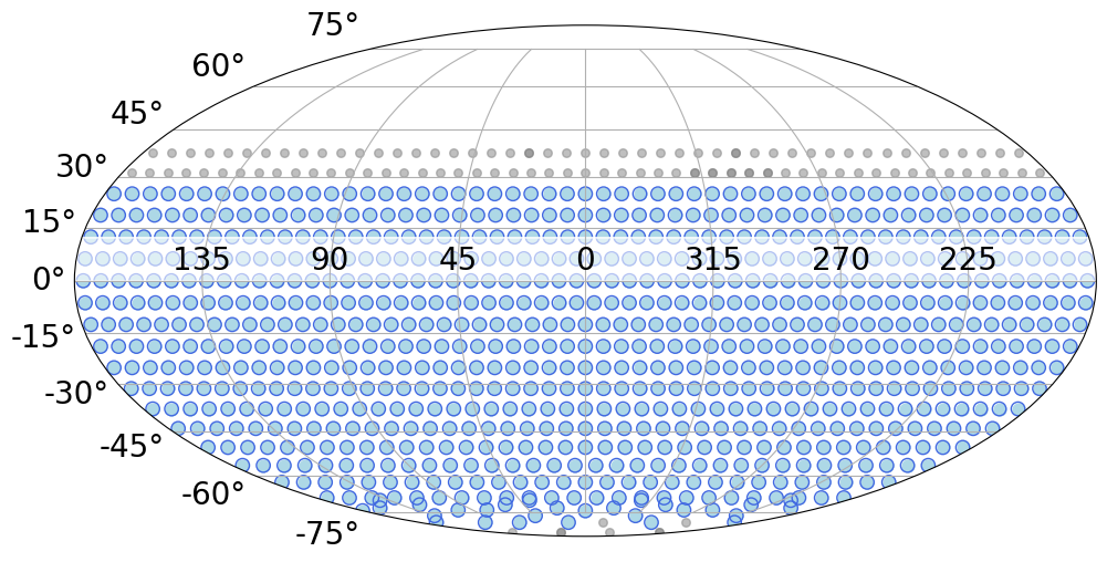
Figure 2: Coverage of tiles used in the first Stokes I catalogue for RACS. Fields that are within the coverage of this first catalogue release are shown in blue. Those fields within the RACS Paper I release that could not be convolved to 25^′′ are shown in grey. In total 799 fields (of a possible 903) contribute to this work. This is presented on an equatorial J2000.0 coordinate frame in Mollweide projection.

2.2 Producing Common Resolution Mosaics

In order to produce images at 25^′′ resolution, we made use of scripts to convolve each of the 36 single beam images to the desired 25^′′ resolution, ensuring retention of the flux scale. This process is discussed further in McConnell et al. (2020). The convolved beam images were then linearly mosaiced together using the ASKAPSoft linmos function. Each beam image was weighted according to the number of contributing visibilities, and linmos assumed a circular Gaussian beam of FWHM $1.09\lambda$/D for the primary beam model of each of the individual 36 beams. Here $\lambda$ is the central wavelength of the observations ($=c/\nu=c/887.5$ MHz $\sim$ 34cm) and D is the diameter of an ASKAP dish (12 m).

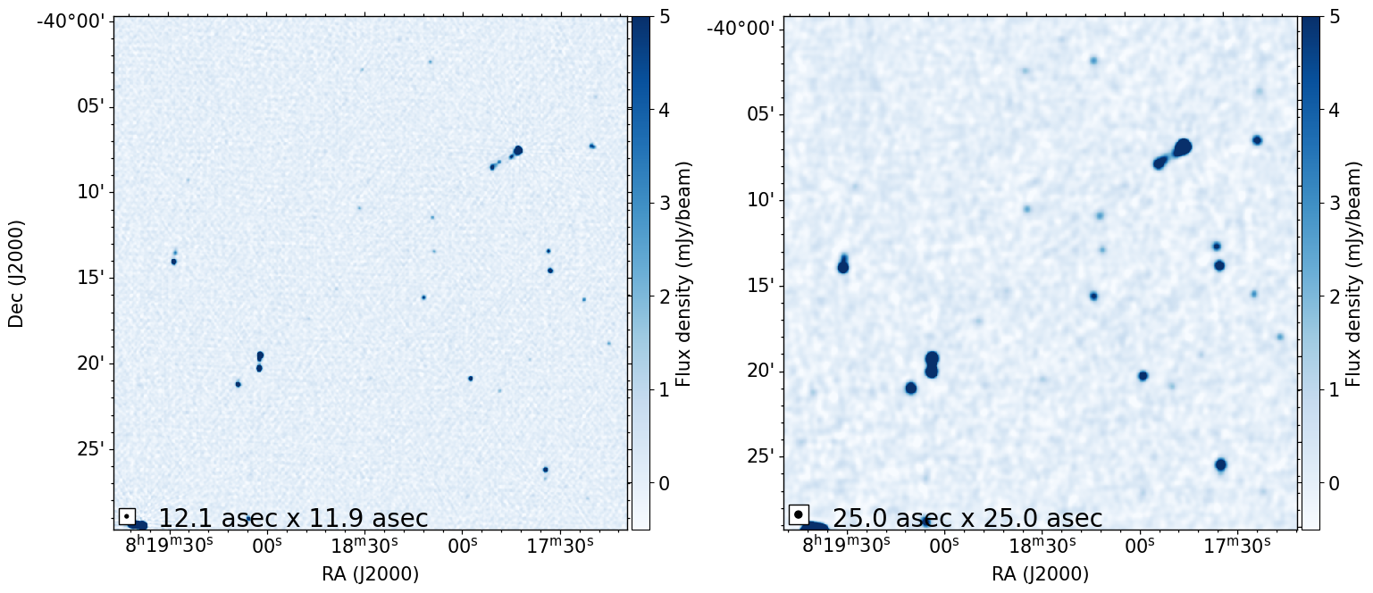
(a) RACS_0810-37A - Beam 27

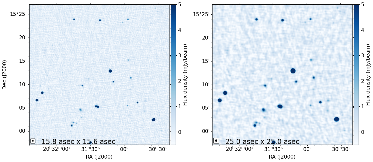
(b) RACS_2037+12A - Beam 17

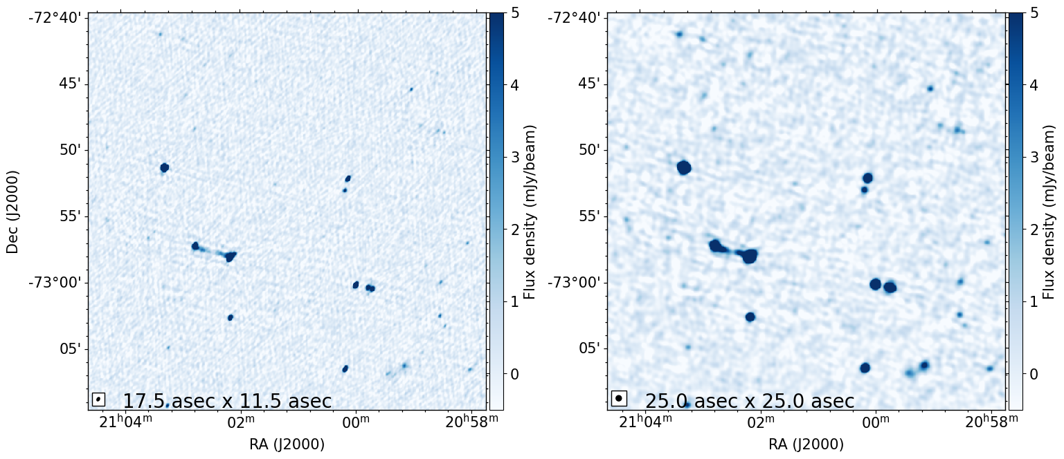
(c) RACS_2100-76A - Beam 16

Figure 3: Example comparison images of (left) the original beam image (pre-mosaicing) compared to (right) those in the 25^′′ mosaic tile image. This is shown for three fields with different angular resolutions (shown in the bottom left of each image). The colour scale for each image varies in the range $-$0.5 to 5 mJy/beam. Shown are tiles: RACS_0810-37A, beam 27 (top); RACS_2037+12A, beam 17 (middle); RACS_2100-76A, beam 16 (bottom).

Figure 3 presents images before and after convolution to 25^′′ resolution for three example regions, showing the differences in images for a range of pre-convolution major axis sizes. As can be seen, convolving to a poorer resolution loses some of the fine structure that could have been observed in the sources, such as in the jets of AGN, and has led to an apparent increase in the rms for each image. However, it does provide a consistent resolution across the full region used for this first Stokes I catalogue data release. This prioritises having a reliable flux scale across the image over retaining higher, but variable, angular resolution (which is still available for all tiles in CASDA).

2.3 Tile Flux Corrections

As discussed in Paper I, the primary beam model assumed by linmos differs from the beam-dependent shapes revealed by holography measurements across the full ASKAP tile. This resulted in systematic and direction dependent errors in the brightness scale. Using a combination of holography and comparisons to SUMSS and NVSS, an empirical flux correction is applied to each tile. We apply this same flux correction to our linearly mosaiced, common resolution tiles. This flux correction varies across the field to a maximum correction of $\sim\pm 30-40\%$.

2.4 Full image mosaic

We mosaiced the convolved 25^′′, flux corrected tiles to improve the sensitivity at the edge of each tile. For each tile, adjacent tiles with overlapping regions were mosaiced together using SWARP (Bertin et al., 2002) using the weights images produced with linmos. The resultant mosaiced tile image has the same extent as the original tile image but now includes contributions from neighbouring tiles. Since all tiles undergo the same mosaicing process, neighbouring mosaiced tiles will contain overlap regions with identical image data.

These mosaiced tiles allow users to extract images over small specific regions with ease, compared to if a full mosaic of the entire sky existed. These mosaics as well as the source catalogue will be released on CASDA alongside the release of the paper. Additionally, as a full image of the sky is important to be able to easily navigate the survey and search for objects, this is included in the form of a HiPS (Fernique et al., 2015) image at https://www.atnf.csiro.au/research/RACS/CRACS_I2/. This HiPS image is an under-sampled version of the mosaiced images that are being released and allows a simple method for users to explore the entire RACS observations.

These mosaiced images of the tiles form the basis of the Stokes I RACS catalogue.

3 Stokes I Catalogue: Individual Tiles

In order to generate the first full Stokes I catalogue of the area described in Section 2.1, we first produced individual catalogues for each mosaiced tile. Further work was needed to combine these catalogues into a single Stokes I catalogue. In this Section, we describe the process of extracting the initial catalogues. The merger of the tile catalogs is then described in Section 4.

We make use of the source extraction software PyBDSF (using version 1.9.1, Mohan & Rafferty, 2015). PyBDSF was designed as a radio source finding tool for the LOw Frequency ARray (LOFAR; van Haarlem et al., 2013) that identifies areas of radio emission (islands) and fits these regions with 2D elliptical Gaussian components in order to produce both a ‘Gaussian component’ and ‘Source’ catalogue. The ‘Gaussian component’ catalogue (hereafter called component) consists of all the 2D Gaussians that are used to model sources in the field. As radio sources have a diverse range of morphologies, a combination of single and multiple component sources will exist within the catalogue. The source catalogue, in its default mode, joins together Gaussians within an island based on the separation of Gaussians and their flux values. Because of this, Gaussians within the same island may be considered different sources. However, if necessary, it is also possible to force Gaussians of the same island to be grouped together in a single source. Details of PyBDSF and the parameters which users can specify can be found at https://www.astron.nl/citt/pybdsf/.

When using PyBDSF on individual tiles, we specified several non-default parameters:

     - advanced_opts = True
     - thresh = ‘hard’
     - rms_box = (150,30)
     - atrous_do = True
     - atrous_jmax = 3
     - mean_map = ‘zero’
     - frequency = 887.5e6
     - group_by_isl = True.

By default, PyBDSF uses a 3$\sigma$ detection threshold to identify an island boundary (thresh_isl = 3), and a 5$\sigma$ threshold is used to include islands within a catalogue (thresh_pix = 5). Setting thresh = ‘hard’ enforces this 5$\sigma$ cut, and does not include a variable threshold based on the false detection rate.

We also specify the box size used by PyBDSF to generate an rms map through specifying rms_box = (150,30). Whilst PyBDSF can internally determine an appropriate size of box in order to produce the rms image, this may need to be changed if there are artefacts within the image. In fact, when we did not specify this parameter, the box size determined by PyBDSF could be as large as approximately 1000 pixels across. This was found to be too large and artefacts around bright sources were being included by PyBDSF in the output catalogue produced. Therefore we decided to specify a smaller box size to better account for bright sources and remove the likelihood of artefacts being confused for real sources. The 150 in the rms box size represents the box size used to calculate the rms. It was chosen to be 150 pixels as this appeared to reflect the scale over which artefacts influenced the image surrounding a bright source for the areas with artefacts investigated. The 30 in rms_box reflects the step size (in pixels) by which the box is moved to calculate the rms.

Moreover, because of the sensitivity of ASKAP to extended emission, we wanted to ensure that such sources were accurately modelled by PyBDSF. To do this we followed advice from the PyBDSF pages. We set the mean_map parameter to ‘zero’ and switched on the atrous mode using atrous_do = True. We used fitting up to three wavelet scales in this mode through setting atrous_jmax = 3. This allows extended emission on larger scales to be fit. As the rms appeared to vary across the field especially around bright sources, we left the rms_map as the default parameter in which an rms map is calculated for the field using the rms box size specified.

Finally, due to the source density within these observations, we believe we are not limited by confusion (see Section 4.2 for more details on the source density). By setting group_by_isl = True, we made the assumption that all sources within the same island are likely associated with the same source. From visually investigating a handful of random fields, the models produced by PyBDSF seemed to model source emission of resolved sources well.

After running PyBDSF we recorded three things:

• The catalogue of Gaussians identified within the image

• The catalogue of grouped sources identified within the image

• An rms image of the field

Both the ‘Gaussian’ and ‘Source’ catalogues have scientific value. The Gaussian catalogue is useful as it can be used to de-blend the emission from close neighbouring sources which are not associated with one another. However, the ‘Source’ catalogue is useful for providing information on multi-component sources. Therefore we construct and release both a ‘Gaussian’ and ‘Source’ catalogue associated with the data.

4 Full Sky Catalogue

We compose the catalogue from the PyBDSF outputs giving each entry a unique identifier by combining field name and PyDBSF source/component identifiers. For example, source 0 in tile RACS_0000+12A was renamed from a Src_ID of 0 to RACS_0000+12A_0. An extra column that included the Tile_ID associated with a source and its separation from the tile centre was also recorded.

Due to the overlapping tiles, a simple concatenation of all the individual catalogues would result in the duplication of sources. As the images within the overlap regions are identical, only sources detected in a given tile for which that tile centre is the closest to the source are included in the final catalogue. The source position, not the position of individual components, is used for this match. This is due to the possibility of different Gaussians within the same source near a tile boundary having different tile centres as their nearest tile. After concatenation, we ensure that no sources from different tiles were separated by less than 2 pixels (i.e. 5^′′). This only affected a very small number of sources (3 pairs - i.e. 6 sources), and so duplicates of these were removed.

We rounded the data to a given number of decimal places for the column also apply another 5$\sigma$ thresholding. Whilst PyBDSF uses a 5$\sigma$ threshold, this will be based on the peak pixel value within the image, not the modelled peak flux. This can therefore be greatly affected by noise fluctuations. To ensure we have high SNR sources we therefore ensure a 5$\sigma$ cut using the peak flux recorded in the PyBDSF catalogue and the island rms column.

Combining components and sources in this manner produced an initial source catalogue over the majority of the southern sky ($\delta=-80$^∘ to $+30$^∘) of $\sim$ 2.3 million  radio sources and a corresponding component catalogue of $\sim$ 2.7 million  components, covering a total sky area of 30,480 deg². Figure 4 presents the observed density of sources across the sky using a HEALPix grid, with an N_side value of 64, corresponding to a rough pixel size of 55^′. The apparent source density variation is discussed later in this paper.

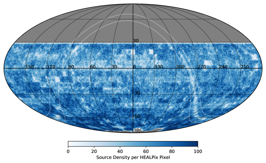
Figure 4: Number density of sources per HEALPix pixel (each approximately 55^′ in size) across the sky from the merged sky catalogue, including the Galactic plane. The Galactic plane region ($|b|=5$^∘) is indicated by the faint solid white lines. This is presented on an equatorial J2000.0 coordinate frame in Mollweide projection.

4.1 Noise Distribution

When PyBDSF produces the source and Gaussian catalogue of each tile, a variable rms map of each image is generated. In order to present this rms variation across this first data release, we randomly select 10 million positions across the sky in the range $\delta=-$85^∘ to +30^∘. At each position, the value of the rms at that location is recorded. We plot this distribution of rms in Figure 5 on the same HEALPix grid as above and plotting the median rms value within each HEALPix cell.

The rms varies across the RACS survey due to a combination of factors. This includes the proximity to bright sources, unmodelled extended emission (which may be a factor close to the Galactic plane), conditions such as the hour angle coverage of the observations and the overlap of tiles across the sky. As shown in Figure 5, there are large rms values along the Galactic plane as well as in other regions for example around $\delta=0$^∘. These variations across the full sky will arise from a variety of reasons such as from having extended emission in the Galactic plane; having bright sources with large artefacts within a field and, finally, the scheduling of the observations relative to its hour angle coverage. The median rms is typically smaller at more southerly declinations compared to equatorial regions. This may be influenced by the greater overlap between neighbouring tiles or possibly due to the hour angle coverage of these observations (see Paper I)

The distribution of all rms values (from these random positions) across the field of view (30,480  deg²) can be seen in Figure 6 (left), and the variation of the median rms value as a function of declination within different declination bins can be seen in Figure 6 (right). This is shown both inclusive and exclusive of the Galactic plane. Across the full sky, the rms values typically have a median value of approximately 0.3 mJy/beam, however this is closer to $0.2-0.25$ mJy/beam at $\delta\lesssim-50$^∘ rising to values closer to $0.35-0.4$ mJy/beam near $\delta=$ 0^∘.

Figure 5: rms distribution across the sky based on selecting random positions across the survey region and calculating the median rms in each HEALPix bin. The Galactic plane ($|b|=5$^∘) is indicated by the faint solid white lines. This is presented on an equatorial J2000.0 coordinate frame in Mollweide projection.

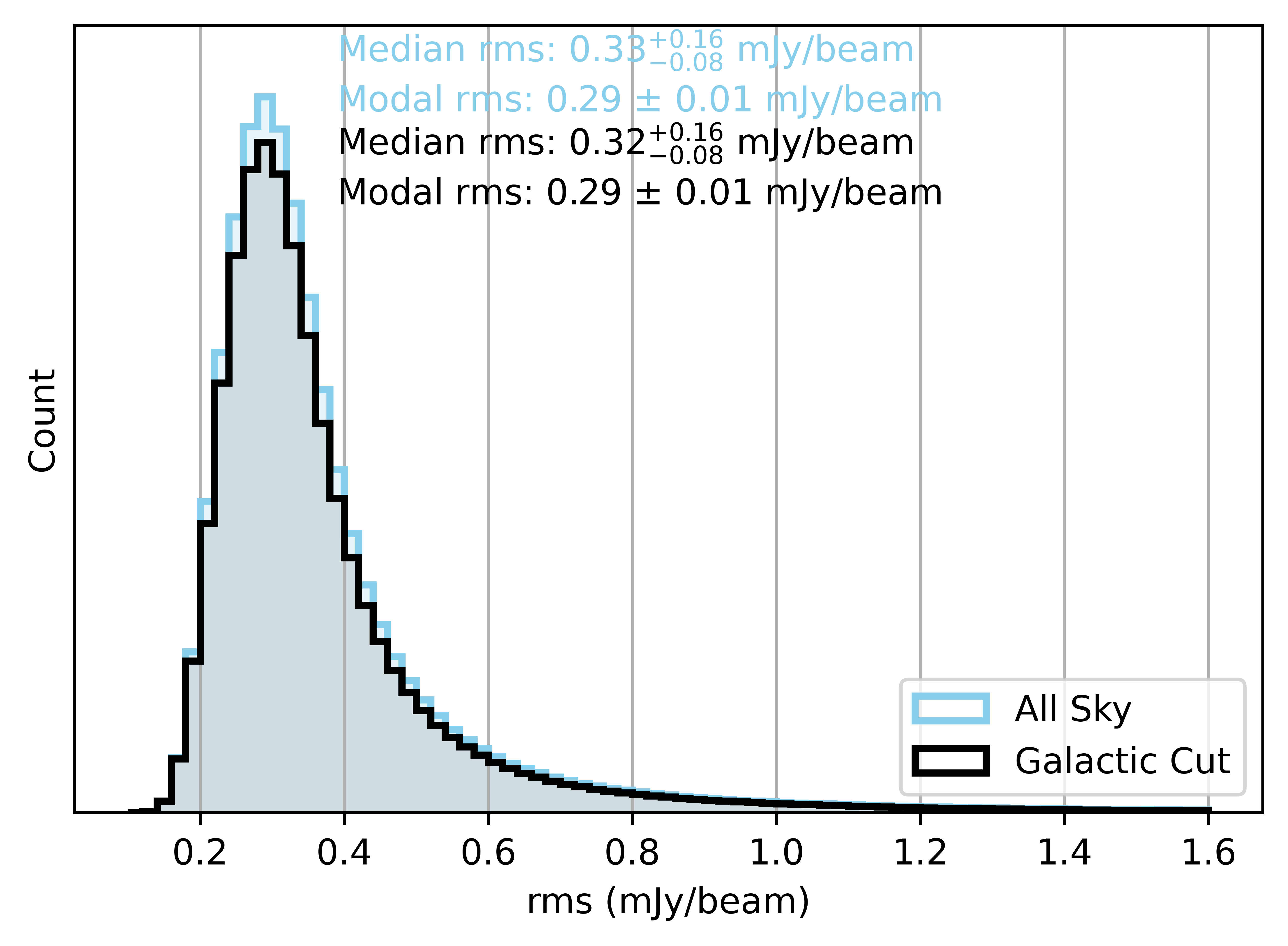
(a)

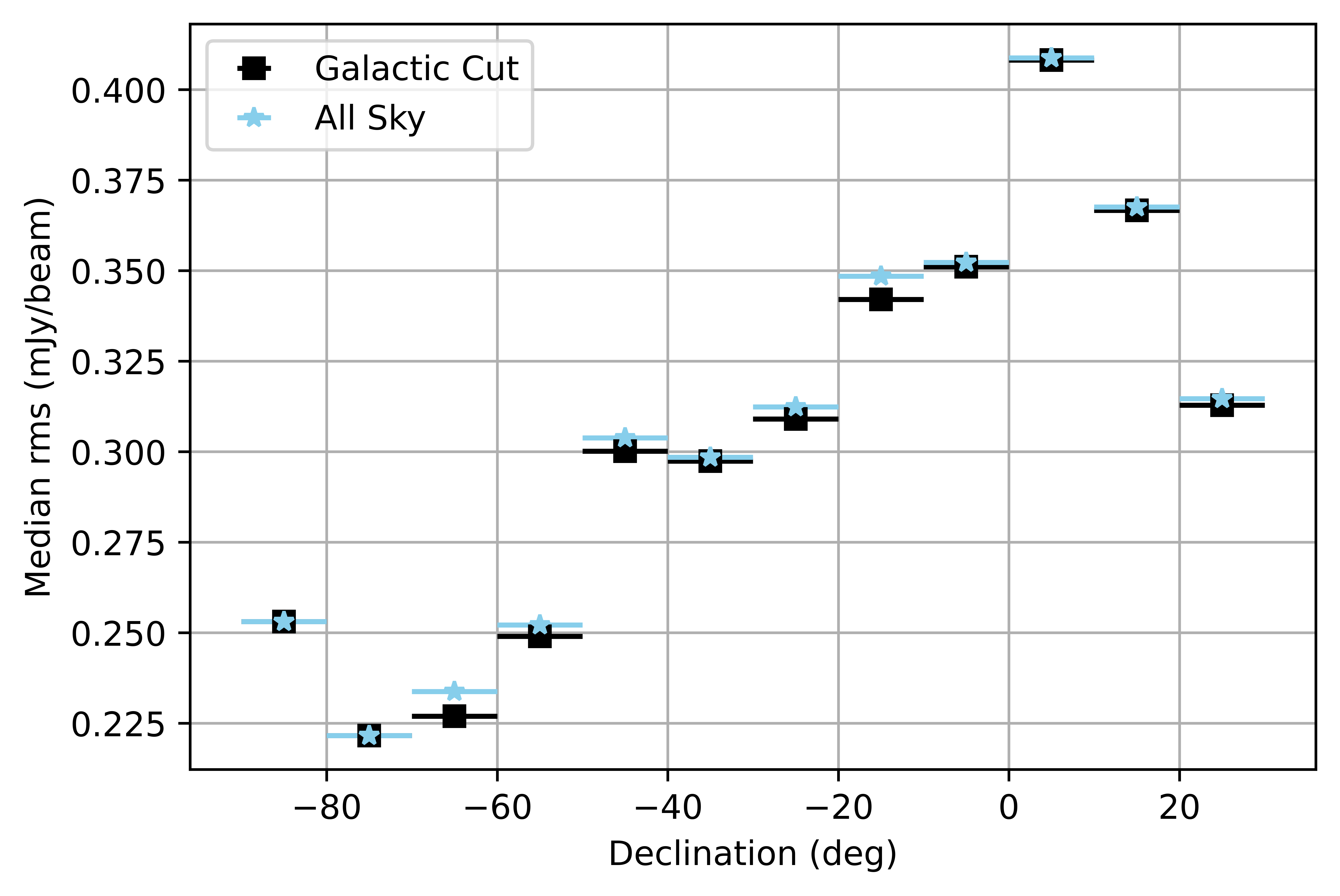
(b)

Figure 6: Left: Histogram of the rms distribution from randomly selecting positions across the sky. Right: The median rms of each declination strip as a function of declination with (blue) and without (black) the Galactic plane included.

4.2 The Galactic Plane

As can be seen in Figure 5, the rms is elevated around the Galactic plane. Furthermore, as presented in Paper I, the emission around the Galactic plane includes substantial extended emission, such as supernova remnants. As these structures will be insufficiently modelled using Gaussian components, we removed the region around the Galactic plane. Therefore whilst the images on CASDA will contain these regions, the final catalogues used for the analysis in this paper do not contain any sources where the magnitude of the Galactic latitude, $|b|<5$^∘. Also, in regions near the Large and Small Magellanic Clouds or supernova remnants sources may be poorly modelled as Gaussian components, however these regions remain in the catalogue.

After excluding the low Galactic latitudes the final source catalogue contains 2,123,638 sources and 2,462,693 Gaussian components over $\sim$28,020 sq. deg of the sky. This corresponds to an average $\sim$90 components or $\sim$75 sources per square degree.

We include with the data release the catalogue generated within the galactic plane region defined here. However, we urge caution for any users wanting to use this catalogue for regions with $|b|<5$^∘. All further quality assessment and comparison of the catalogue to previous surveys refers solely to the catalogue with the galactic latitude cut imposed and we note that, as can be seen in McConnell et al. (2020), there may be flux density offsets close to the galactic field, as well as large RMS values (see Figure 6).

4.3 Catalogue Columns

Using the combined PyBDSF catalogues, we use a subset of the column information when generating the final catalogues. These columns provide information on: IDs; astrometry; flux densities; shape information and other important source information. We present an example of the first 10 lines of the source catalogue in Table 2 and Gaussian component catalogue in Table 3, sorted by the Source_ID of the source/Gaussian component. We present a description of the column information for these two RACS Stokes I catalogues below.

Source_Name	Source_ID	Tile_ID	SBID	Obs_Start_Time
RACS-DR1 J001237.8+101809	RACS_0000+12A_1071	RACS_0000+12A	8578	58599.06929
RACS-DR1 J001237.3+101939	RACS_0000+12A_1072	RACS_0000+12A	8578	58599.06929
RACS-DR1 J001236.9+110238	RACS_0000+12A_1079	RACS_0000+12A	8578	58599.06929
RACS-DR1 J001234.3+110628	RACS_0000+12A_1084	RACS_0000+12A	8578	58599.06929
RACS-DR1 J001231.2+103907	RACS_0000+12A_1088	RACS_0000+12A	8578	58599.06929
RACS-DR1 J001232.9+114652	RACS_0000+12A_1089	RACS_0000+12A	8578	58599.06929
RACS-DR1 J001234.1+124520	RACS_0000+12A_1090	RACS_0000+12A	8578	58599.06929
RACS-DR1 J001235.3+134158	RACS_0000+12A_1092	RACS_0000+12A	8578	58599.06929
RACS-DR1 J001228.3+112827	RACS_0000+12A_1098	RACS_0000+12A	8578	58599.06929
RACS-DR1 J001226.8+105716	RACS_0000+12A_1100	RACS_0000+12A	8578	58599.06929

N_Gaus	RA	Dec	E_RA	E_DEC	Total_flux	E_Total_flux	E_Total_flux	Peak_flux
					_Source	_Source_PyBDSF	_Source
	∘	∘	′′	′′	mJy	mJy	mJy	mJy/beam
1	3.157688	10.302451	1.75	1.04	3.560	0.666	1.003	2.968
1	3.155227	10.327487	0.24	0.23	14.890	0.562	1.642	14.881
1	3.153751	11.043854	3.45	4.50	7.158	1.613	1.898	2.060
1	3.142925	11.107845	1.10	1.26	3.163	0.628	0.957	3.318
1	3.129824	10.652017	1.67	2.52	2.563	0.695	0.972	1.971
1	3.137132	11.781003	1.71	1.32	4.822	0.889	1.222	3.460
1	3.142223	12.755545	2.17	1.26	13.814	1.632	2.195	5.772
1	3.147178	13.699465	0.05	0.05	73.474	0.572	5.672	71.689
1	3.117901	11.474149	0.11	0.11	41.977	0.760	3.521	40.863
1	3.111569	10.954526	2.36	2.15	2.343	0.752	1.003	2.020

E_Peak_flux	Maj	E_Maj	Min	E_Min	PA	E_PA	DC_Maj	E_DC_Maj	DC_Min
mJy/beam	′′	′′	′′	′′	∘	∘	′′	′′	′′
0.336	32.24	4.23	23.31	2.27	105.09	17.11	0.00	4.23	0.00
0.324	25.44	0.56	24.64	0.53	80.74	29.91	0.00	0.56	0.00
0.368	60.15	12.06	36.16	5.76	33.30	20.82	54.70	12.06	26.12
0.374	25.58	3.03	23.33	2.50	158.81	51.49	0.00	3.03	0.00
0.334	31.86	5.95	25.56	3.92	0.26	35.41	19.73	5.95	5.13
0.407	32.56	4.16	26.79	2.91	111.73	27.96	20.82	4.16	9.61
0.495	53.55	5.57	27.97	1.98	116.00	8.56	47.34	5.57	12.54
0.325	25.49	0.12	25.17	0.11	100.85	17.02	4.79	0.12	2.89
0.431	25.47	0.27	25.25	0.26	154.41	43.48	4.85	0.27	3.27
0.392	28.78	5.94	25.24	4.60	124.68	64.18	14.23	5.94	3.17

E_DC	DC_PA	E_DC_PA	S_Code	Separation	Noise	Gal_lon	Gal_lat	Flag
_Min				_Tile_Centre				_Close
′′	∘	∘		∘	mJy/beam	∘	∘
2.27	0.00	17.11	S	3.8431	0.329	107.518268	-51.404165	-
0.53	0.00	29.91	S	3.8262	0.324	107.524147	-51.379281	-
5.76	33.30	20.82	S	3.4484	0.367	107.793667	-50.683253	-
2.50	0.00	51.49	S	3.4105	0.379	107.801283	-50.618566	-
3.92	0.26	35.41	S	3.6220	0.319	107.609691	-51.058232	-
2.91	111.73	27.96	S	3.1691	0.385	108.040448	-49.962954	-
1.98	116.00	8.56	S	3.0707	0.488	108.394965	-49.015996	-
0.11	100.85	17.02	S	3.2624	0.323	108.725686	-48.097792	-
0.26	154.41	43.48	S	3.2441	0.428	107.899652	-50.256826	-
4.60	124.68	64.18	S	3.4531	0.380	107.696621	-50.760190	-

Table 2: The first 10 lines from the final source catalogue. The columns are described in Section 4.3.1.

Gaussian_ID	Source_ID	Tile_ID	SBID	Obs_Start_Time	N_Gaus	RA
						∘
RACS_0000+12A_1243	RACS_0000+12A_1071	RACS_0000+12A	8578	58599.06929	1	3.157688
RACS_0000+12A_1244	RACS_0000+12A_1072	RACS_0000+12A	8578	58599.06929	1	3.155227
RACS_0000+12A_1251	RACS_0000+12A_1079	RACS_0000+12A	8578	58599.06929	1	3.153751
RACS_0000+12A_1256	RACS_0000+12A_1084	RACS_0000+12A	8578	58599.06929	1	3.142925
RACS_0000+12A_1260	RACS_0000+12A_1088	RACS_0000+12A	8578	58599.06929	1	3.129824
RACS_0000+12A_1261	RACS_0000+12A_1089	RACS_0000+12A	8578	58599.06929	1	3.137132
RACS_0000+12A_1262	RACS_0000+12A_1090	RACS_0000+12A	8578	58599.06929	1	3.142223
RACS_0000+12A_1265	RACS_0000+12A_1092	RACS_0000+12A	8578	58599.06929	1	3.147178
RACS_0000+12A_1272	RACS_0000+12A_1098	RACS_0000+12A	8578	58599.06929	1	3.117901
RACS_0000+12A_1274	RACS_0000+12A_1100	RACS_0000+12A	8578	58599.06929	1	3.111569

Dec	E_RA	E_Dec	Total_flux	E_Total_flux	E_Total_flux	Total_flux	E_Total_flux	E_Total_flux
			_Gaussian	_Gaussian	_Gaussian	_Source	_Source	_Source
				_PyBDSF			_PyBDSF
∘	′′	′′	mJy	mJy	mJy	mJy	mJy	mJy
10.302451	1.75	1.04	3.560	0.666	1.003	3.560	0.666	1.003
10.327487	0.24	0.23	14.890	0.562	1.642	14.890	0.562	1.642
11.043854	3.45	4.50	7.158	1.613	1.898	7.158	1.613	1.898
11.107845	1.10	1.26	3.163	0.628	0.957	3.163	0.628	0.957
10.652017	1.67	2.52	2.563	0.695	0.972	2.563	0.695	0.972
11.781003	1.71	1.32	4.822	0.889	1.222	4.822	0.889	1.222
12.755545	2.17	1.26	13.814	1.632	2.195	13.814	1.632	2.195
13.699465	0.05	0.05	73.474	0.572	5.672	73.474	0.572	5.672
11.474149	0.11	0.11	41.977	0.760	3.521	41.977	0.760	3.521
10.954526	2.36	2.15	2.343	0.752	1.003	2.343	0.752	1.003

Peak_flux	E_Peak_flux	Maj	E_Maj	Min	E_Min	PA	E_PA	DC_Maj	E_DC_Maj	DC_Min
mJy/beam	mJy/beam	′′	′′	′′	′′	∘	∘	′′	′′	′′
2.968	0.336	32.24	4.23	23.31	2.27	105.09	17.11	0.00	4.23	0.00
14.881	0.324	25.44	0.56	24.64	0.53	80.74	29.91	0.00	0.56	0.00
2.060	0.368	60.15	12.06	36.16	5.76	33.30	20.82	54.70	12.06	26.12
3.318	0.374	25.58	3.03	23.33	2.50	158.81	51.49	0.00	3.03	0.00
1.971	0.334	31.86	5.95	25.56	3.92	0.26	35.41	19.73	5.95	5.13
3.460	0.407	32.56	4.16	26.79	2.91	111.73	27.96	20.82	4.16	9.61
5.772	0.495	53.55	5.57	27.97	1.98	116.00	8.56	47.34	5.57	12.54
71.689	0.325	25.49	0.12	25.17	0.11	100.85	17.02	4.79	0.12	2.89
40.863	0.431	25.47	0.27	25.25	0.26	154.41	43.48	4.85	0.27	3.27
2.020	0.392	28.78	5.94	25.24	4.60	124.68	64.18	14.23	5.94	3.17

E_DC	DC_PA	E_DC	S_Code	Separation	Noise	Gal_lon	Gal_lat
		_PA		_Tile_Centre
′′	∘	∘		∘	mJy/beam	∘	∘
2.27	0.00	17.11	S	3.8431	0.329	107.518268	-51.404165
0.53	0.00	29.91	S	3.8262	0.324	107.524147	-51.379281
5.76	33.30	20.82	S	3.4484	0.367	107.793667	-50.683253
2.50	0.00	51.49	S	3.4105	0.379	107.801283	-50.618566
3.92	0.26	35.41	S	3.6220	0.319	107.609691	-51.058232
2.91	111.73	27.96	S	3.1691	0.385	108.040448	-49.962954
1.98	116.00	8.56	S	3.0707	0.488	108.394965	-49.015996
0.11	100.85	17.02	S	3.2624	0.323	108.725686	-48.097792
0.26	154.41	43.48	S	3.2441	0.428	107.899652	-50.256826
4.60	124.68	64.18	S	3.4531	0.380	107.696621	-50.760190

Table 3: The first 10 lines from the final Gaussian component catalogue. The columns are described in Section 4.3.2.

4.3.1 Source Catalogue

For the Source catalogue, we define the following columns:

• Source_Name - The name of the source given in the IAU convention JHHMMSS.S$\pm$DDMMSS with the prefix RACS-DR1

• Source_ID - The ID of the source given by the RACS tile ID added to the Src_ID generated by PyBDSF

• Tile_ID - The ID of the tile that the source was located in.

• SBID - The ID of the scheduling block associated with the observation.

• Obs_Start_Time - The time that the pointing observation started as Modified Julian Day (MJD) expressed in days.

• N_Gaus - The number of Gaussian components that were used to fit the source

• RA and Dec (and errors) - The J2000 position of the source and its associated errors

• Total_flux_Source - The total flux density of the entire source (i.e. the sum of the Gaussian components and the Total_Flux column in the PyBDSF source catalogue).

• E_Total_flux_Source_PyBDSF - The error on the total flux density from the E_Total_Flux column in PyBDSF.

• E_Total_flux_Source - The combined error on the total flux density derived by summing in quadrature the error from PyBDSF with the errors of flux density from Equation 7 of McConnell et al. (2020).

• Peak_flux (and error) - The modelled peak flux density for the source and its associated error from PyBDSF

• Maj, Min and PA (and errors) - The major axis, minor axis and position angle of the source fit by PyBDSF

• DC_Maj, DC_Min and DC_PA (and errors) - The deconvolved major axis, minor axis and position angle of the source

• S_Code - The code from PyBDSF which defines whether a source is a single (S), multiple (M) or complex (C) source. A single source (S) is a single Gaussian source corresponding to a single island. A multiple (M) is where a single source is comprised of multiple Gaussians. A complex source (C) is a source where there are multiple Gaussians which form multiple sources within an island.

• Separation_Tile_Centre - The distance between the source and the centre of the tile it is located in.

• Noise - The rms noise within the island boundary, quoted from the Isl_rms column in PyBDSF.

• Gal_lon and Gal_lat - The Galactic longitude and latitude of the source in degrees

• Flag_Close - All sources where there was another source within 25^′′ are flagged with a ‘C’. For 2 pairs of sources, these were so closely located that the Source_Name was identical. This is only 2 Source_Name’s out of $\sim$2 million and so we have flagged these with ‘CD’ in this column. For Sources with no match within 25^′′ have ‘-’ in this column.

Unless specified, associated are as described in the PyBDSF documentation.

4.3.2 Gaussian Component Catalogue

For the Gaussian component catalogue, the associated columns are:

• Gaussian_ID -The ID corresponding to the Gaussian component constructed as the RACS tile ID added to a unique Gaussian ID for the Gaussian components in the individual tile

• Source_ID, Tile_ID, SBID, Obs_Start_Time and N_Gaus - as above, describing the source associated with this Gaussian component

• RA/Dec (and errors) - The J2000 position of the Gaussian component and its associated errors

• Total_Flux_Gaussian (and errors) - The modelled total flux density of each individual Gaussian component and the associated errors (similar to as described above for the source but now for the component flux density).

• Total_Flux_Source (and errors) - Total flux densities and errors as described for the source catalogue

• Peak_Flux (and error) - The modelled peak flux density of the Gaussian component and its associated error.

• Maj/Min/PA (and error) - The major and minor axes of the source (FWHM) and the position angle of the Gaussian component used to model the source

• Maj_DC/Min_DC/PA_DC (and errors) - The deconvolved source sizes and position angle of the Gaussian component

• S_Code - as in source catalogue

• Separation_Tile_Centre - The distance between the Gaussian component and the centre of the pointing it is located in

• Noise - as in source catalogue

• Gal_lon and Gal_lat - The Galactic longitude and latitude of the Gaussian component

More information on how the parameters in the source (*srl.fits) and Gaussian component (*gaul.fits) catalogues are produced by PyBDSF can be found through the PyBDSF documentation.

We note here that other work may use differing terminology to the source/Gaussian definitions used in this work. For example, “source" in other work may refer to the final radio object where separated lobes and components that have not been identified by PyBDSF as differing sources but that actually come from the same physical object are combined together. This process of combining “sources" (as defined here) into the same physical object often relies on a combination of visual identification and either machine learning methods or likelihood ratios (see e.g. Banfield et al., 2015; Williams et al., 2019; Galvin et al., 2020). The process of combining sources into objects for RACS, however, is beyond the scope of this work.

5 Comparisons with Previous Radio Surveys

Having completed the construction of a final catalogue, we now make comparisons with previous radio surveys at various radio frequencies in order to validate the values determined from RACS.

5.1 Comparison Images

We begin with a visual comparison for a handful of RACS sources and their counterpart regions in SUMSS, NVSS and TGSS-ADR, to indicate the difference in image resolution and baseline sensitivity. We include a comparison image from the IR wavelength AllWISE survey (Cutri & et al., 2013), to make comparisons for a nearby resolved galaxy. As all these surveys have different sky coverage, there is only a narrow declination window ($\delta=-$40^∘ to $-$30^∘) where it is possible to make a comparison with all four surveys. To obtain these images we make use of the cutout servers for each of the respective surveys.

Figure 7 demonstrates the higher resolution and increased sensitivity of RACS compared to SUMSS and NVSS. The sensitivity of ASKAP to extended emission is shown to be especially important (see the upper panel) to observe the structure in the spiral arms of the resolved galaxy NGC2997. These four cutouts highlight the improvement of RACS on previous large sky southern radio surveys. These images aim to indicate the quality that can be achieved with RACS. On the other hand, there may be regions, for example around bright sources, with poorer sensitivity compared to other surveys due to the snapshot nature of these observations and difficulties with the image processing.

Images in these regions will be improved with further observations of RACS as well as in the future with surveys such as the Evolutionary Map of the Universe (EMU; Norris et al., 2011; Norris et al., 2021).

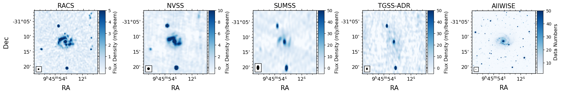
Figure 7: Comparison images between RACS at 25^′′ (left), NVSS (centre left), SUMSS (centre), TGSS-ADR (centre right) and AllWISE W1 band (right) around four sources within the declination range $-$40^∘ to $-$30^∘. The box in the bottom left of each panel indicates the PSF size for each observation. The flux density scales varies from image to image depending on its sensitivity.

5.2 Flux Offsets, Astrometric Offsets and Spectral Indices

It is important to ensure an accurate flux scale and accurate astrometry compared to previous observations as well as to investigate how the measured spectral index compares to our knowledge of the radio source population. We therefore compare our results to five previous large area radio surveys: GLEAM, NVSS, SUMSS and TGSS-ADR. Each of these surveys have different angular resolutions, operate at different frequencies and observe different (although often overlapping) regions of sky. Due to the differences in resolution and sensitivity, we restrict comparison to unresolved, high signal-to-noise, isolated sources. This ensures differences in the angular resolution, noise and sensitivity to extended emission do not affect our comparisons.

5.2.1 Identifying Unresolved Sources

To select unresolved sources we follow a previously-employed method (Bondi et al., 2008; Smolčić et al., 2017a; Shimwell et al., 2019) by defining an envelope to distinguish unresolved sources from those which are resolved. To construct this envelope, we used the Gaussian component catalogue and selected those components that were classified as single sources, and detected at SNR$\geq$5, where the SNR was defined as the peak flux of the Gaussian component divided by its island rms noise. We then considered how the ratio of the integrated flux density ($S_{T}$) to peak ($S_{P}$) flux density as a function of SNR; see Figure 8.

The total flux-density $S_{T}$ of an unresolved source with peak brightness $S_{P}$= $S$ mJy/beam is $S_{T}$ = $S$ mJy, by construction. Therefore, if a source is unresolved and the synthesized beam size is a correct representation of the image resolution, the ratio of the integrated to peak flux ($S_{T}/S_{P}$) should be identically 1. This ratio, however, often has scatter around 1, especially at low SNR where faint sources are more affected by noise at the source position. For our data we find that as the SNR increases, $S_{T}/S_{P}$ tends to a value of 1.025, as illustrated in Figure 8 (right panel). The source of the discrepant value of $S_{T}/S_{P}$ is unimportant for our analysis here, but must lie in some unmodelled source smearing due to effects such as uncorrected gain errors or astrometric mismatches between overlapping beams. Following the methods of (Bondi et al., 2008; Smolčić et al., 2017a; Shimwell et al., 2019) we expect values of $S_{T}/S_{P}$, as a function of SNR, to lie predominantly between the envelopes described by:

$$\frac{S_{T}}{S_{P}}_{\pm}=1.025\pm A\times\textrm{SNR}^{-B}.$$ (1)

As resolved sources will have elevated values of $S_{T}/S_{P}$, we determine values for A, B from the lower envelope $S_{T}/{S_{P}}_{-}$ and declare sources with $S_{T}/S_{P}$ > $S_{T}/{S_{P}}_{+}$ to be resolved. To generate this fit, we use equally spaced logarithmic bins in SNR. For each bin with 100 sources or more, we find the $S_{T}/S_{P}$ ratio that contains 95% of the sources with $S_{T}/S_{P}<1.025$, indicated by the black crosses on Figure 8. These points are fit to Equation 1 using the Scipy function curve_fit. This fit to the lower envelope is determined to be: 1.025 $-$ 0.69 $\times$ SNR^-0.62. We reflect this envelope about $S_{T}/S_{P}$ = 1.025 and define the upper envelope: $S_{T}/S_{P}$ = 1.025 + 0.69 $\times$ SNR^-0.62. Sources below the upper and lower envelopes are determined to be unresolved. Unresolved components are shown as blue points in Figure 8 and resolved sources in grey. From this we estimate approximately 40% of RACS sources are unresolved at 25^′′ resolution, and should therefore also be unresolved in the comparison catalogs.

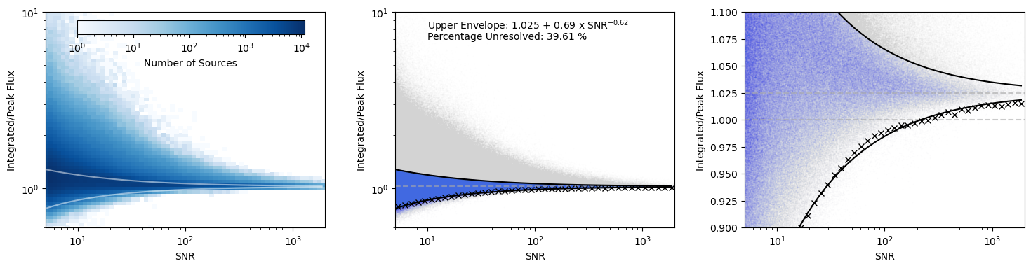
Figure 8: The ratio of integrated to peak flux as a function of SNR for single component sources at $\geq 5\sigma$ and the envelope (grey in left figure; black otherwise) used to define unresolved sources. Points in blue indicate those sources believed to be unresolved and grey indicates those sources believed to be resolved as defined by the envelope described in Section 5.2.1. The black crosses indicates the $S_{T}/S_{P}$ values in which 95% of sources below $S_{T}/S_{P}=1.025$ are included within the envelope. The grey dashed line indicates the ratio $S_{T}/S_{P}=1.025$. The right panel shows a closer view of the left panel around $S_{T}/S_{P}\sim 1$ (also given by a dashed line).

5.2.2 Matching catalogues

For comparison with other catalogues, RACS sources are selected according to the following criteria:

1. Are isolated within an angular separation of $N_{ISO}$^′′. The value of $N_{ISO}$ is given as twice the poorer resolution (using the FWHM) of the two catalogues being compared. We apply the same ‘isolated’ criterion for the comparison radio survey.

2. Have a peak SNR in RACS $\geq 10$

3. Satisfy the unresolved envelope criterion as described above.

4. Match the comparison radio catalogue within an angular separation of $N_{match}$^′′. Here $N_{match}$ is taken to be 10^′′. This value corresponds to 4 pixels in the RACS images and allows for variation in the positions measured of sources, given NVSS and SUMSS have an angular resolution $\sim$2 times poorer than RACS.

The resolution and frequency for each of the surveys we compare to RACS are shown in Table 4. We use sources which satisfy the match criteria to consider the offsets in flux and astrometry, as well as the measured spectral indices. The spectral index ($\alpha$) is used to define the broadband radio emission as a power law of the form $S_{\nu}\propto\nu^{\alpha}$, where $S_{\nu}$ is the flux density at a frequency, $\nu$. Typically $\alpha$ is found in catalogues to have an average value of $-$0.7 to $-$0.8 in the synchrotron dominated regime (see e.g. Condon, 1992; Mauch et al., 2003; Smolčić et al., 2017a).

	AT20G	GLEAM	NVSS	SUMSS	TGSS-ADR	TGSS-ADR-R
Frequency (MHz)	20,000	200 (wide band)	1,400	843	150	150
Resolution (arcsec)	$\sim$10	120	45	$\frac{45}{|\textrm{sin}\delta|}$	25 ($\delta\geq 19^{\circ}$)	25 ($\delta\geq 19^{\circ}$)
					$\frac{25}{\textrm{cos}(\delta-19^{\circ})}$ ($\delta<19^{\circ}$)	$\frac{25}{\textrm{cos}(\delta-19^{\circ})}$ ($\delta<19^{\circ}$)
Assumed 5$\sigma$ Limit (mJy)	-	40	2.5	-	20	20
at observed frequency
N Matches (Flux)	-	-	-	53,680	-	-
Flux Ratio	-	-	-	$1.00^{+0.16}_{-0.16}$	-
N Matches (Astrometry)	2505	-	286,735	53,680	-	-
RA Offset (′′)	$-0.85^{+1.32}_{-1.22}$		$-0.71^{+2.28}_{-2.22}$	$+0.46^{+4.05}_{-3.66}$
Dec Offset (′′)	$+0.21^{+0.77}_{-0.86}$		$+0.31^{+2.31}_{-2.38}$	$+0.12^{+2.51}_{-2.62}$
N Matches	-	24,096	286,735	-	131,258	121,392
(Alpha - No Flux Cut)
Alpha (No Flux Cut)	-	$-0.69^{+0.25}_{-0.21}$	$-0.87^{+0.52}_{-0.42}$	-	$-0.64^{+0.26}_{-0.23}$	$-0.62^{+0.25}_{-0.22}$
N Matches	-	8,795	222,436	-	45,512	41,989
(Alpha - Flux Cut)
Alpha (Flux Cut)	-	$-0.61^{+0.32}_{-0.19}$	$-0.90^{+0.43}_{-0.39}$	-	$-0.59^{+0.36}_{-0.22}$	$-0.58^{+0.36}_{-0.21}$

Table 4: Measured flux density and astrometric offsets, as well as spectral index comparisons between RACS and GLEAM, NVSS, SUMSS and TGSS-ADR as also the rescaled TGSS-ADR (Hurley-Walker, 2017). Offsets are quoted as the median value as well as the associated errors using the 16^th and 84^th percentiles.

5.2.3 Flux Offsets

We make flux density comparisons using SUMSS due to its close proximity in frequency to RACS (843 MHz for SUMSS compared to 887.5 MHz for RACS). This minimizes any effect of spectral index uncertainty on flux density comparisons. For example, assuming a nominal spectral index of $\alpha=-0.8\pm 0.1$ we expect the frequency differences between RACS and SUMSS to result in a flux offset of $\pm 0.5$%, increasing to $\pm$5% at the frequency of NVSS resulting from the error in spectral index.

Using the matching criteria described above, 53,680 matched sources were identified. The comparison of total flux densities assuming a spectral index of $\alpha=-0.8$ can be seen in Figure 9. From this we find a median flux ratio of $1.00^{+0.16}_{-0.16}$. The associated errors are quoted from the 16${}^{\textrm{th}}$ and 84${}^{\textrm{th}}$ percentiles. We therefore conclude that we have an accurate flux scale for our observations. This flux comparison as a function of position can also be seen in Figure 10. We present this for both comparisons with SUMSS (Figure 10, left) but also show this comparison with NVSS (Figure 10, right). Whilst the difference in frequency compared to NVSS is larger, the two figures in Figure 10 combined show the flux offsets across the majority of the coverage of RACS. Figure 10 does not appear to show significant systematic variation in the ratios of flux density as a function of position.

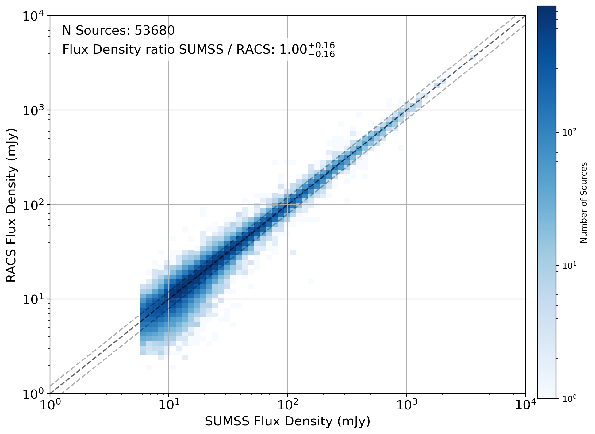
Figure 9: Flux density comparison between RACS and SUMSS at a frequency of 887.5 MHz (assuming $\alpha=-0.8$), for sources matched using the criteria described in Section 5.2.2. The black dashed line indicates a 1-to-1 relation, whilst the grey dashed lines indicate flux ratios of 80 or 120%.

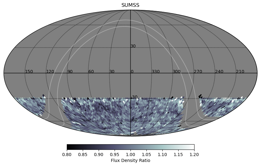
(a) SUMSS

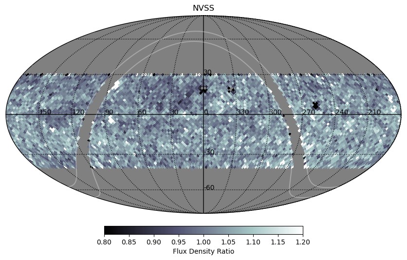
(b) NVSS

Figure 10: Flux density ratio comparison as a function of sky position between RACS and SUMSS (left) at a frequency of 887.5 MHz (assuming $\alpha=-0.8$), for sources as matched per the criteria in Section 5.2.2. We also include the comparison with NVSS (right) to allow for a comparison of the flux density ratio over the full sky.

5.2.4 Astrometric Offsets

We assess the astrometry of RACS, using matches that satisfy the selection criteria described in Section 5.2.2 for some of the catalogues described in Table 4. We define the RA offset to be: $\Delta\textrm{RA}$ = RA${}_{\textrm{RACS}}$- RA${}_{\textrm{Comp}}$ where “Comp” refers to the comparison survey. The Declination offset is defined in the same way. These astrometric offsets can be seen in Figure 11. We compare to SUMSS and NVSS, but not to GLEAM due to its much larger PSF ($\sim$2^′), nor to TGSS-ADR as it was tied to the astrometry of NVSS ($\delta\geq-35$^∘) and MGPS or SUMSS ($\delta\leq-35$^∘) to avoid residual astrometric errors from ionospheric interference at low frequencies. We also include a comparison to AT20G which, although it has far fewer comparison sources than NVSS and SUMSS, provides a comparison with surveys at much higher frequencies.

From this we find small median systematic offsets in both RA and Dec, |Offset|$\lesssim$ 0.8^′′, where the RA value of RACS is systematically lower than NVSS and AT20G but larger than SUMSS. Here we find RA offsets (in ^′′) of: $-0.85^{+1.32}_{-1.22}$ (AT20G), $-0.71^{+2.28}_{-2.22}$ (NVSS) and $+0.46^{+4.05}_{-3.66}$ (SUMSS). The Dec offset is smaller in magnitude than for RA. The measured Dec offsets (in ^′′) are: $+0.21^{+0.77}_{-0.86}$ (AT20G), $+0.31^{+2.31}_{-2.38}$ (NVSS) and $+0.12^{+2.51}_{-2.62}$ (SUMSS). However as the pixel size of the images is 2.5^′′, these offsets are typically constrained within a pixel or two. Further discussion of the beam to beam accuracy in astrometry within the individual beam images can be found in Paper I.

The variation of astrometric offset with sky position can be seen in Figures 12 and 13 for Right Ascension and Declination respectively.

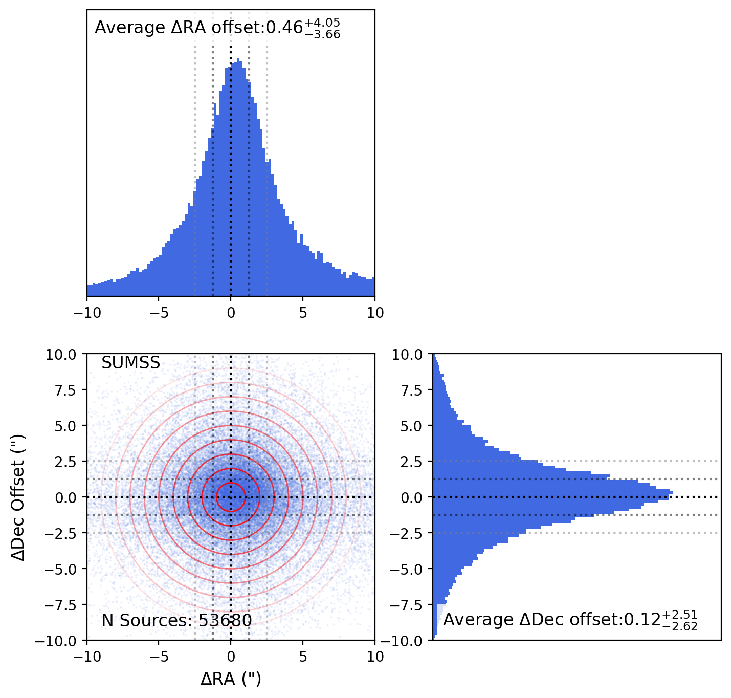
(a) SUMSS

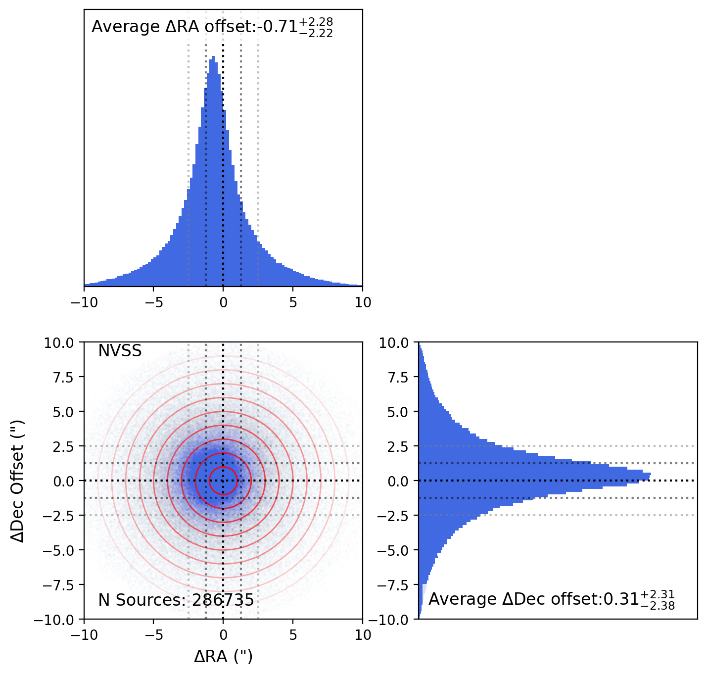
(b) NVSS

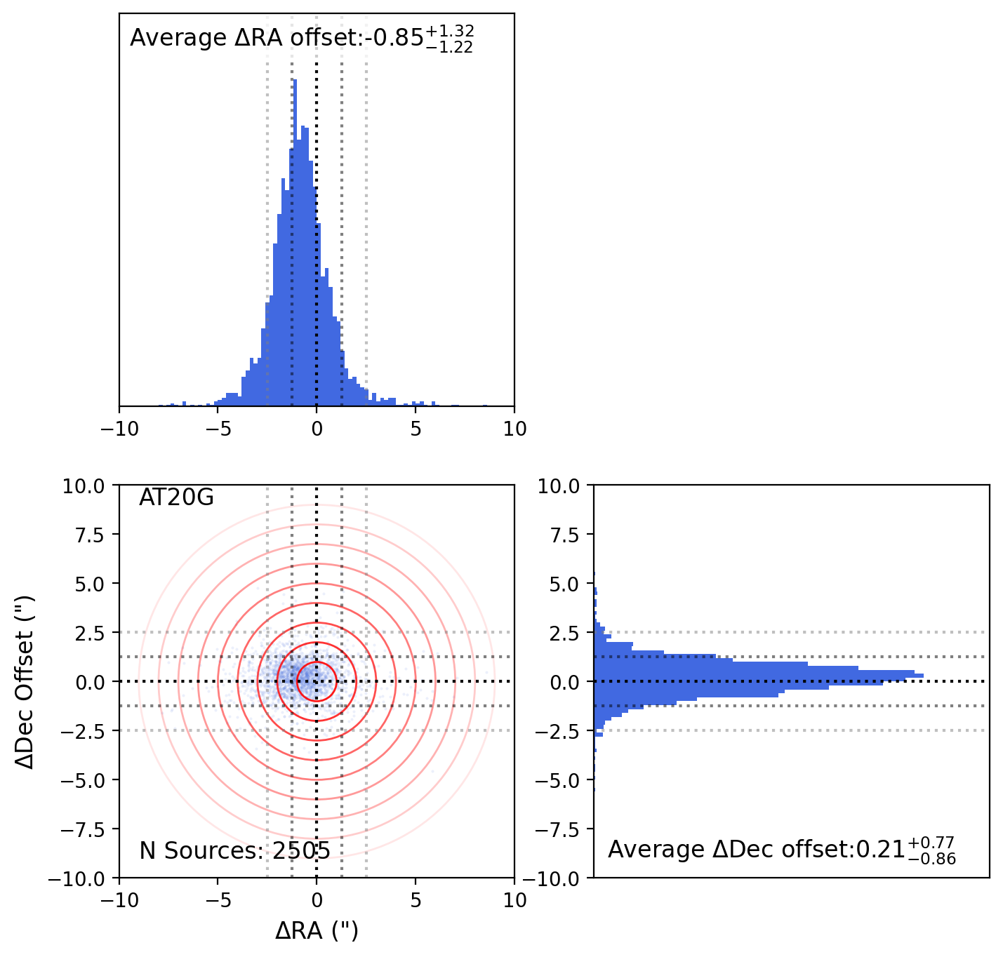
(c) AT20G

Figure 11: Comparison of the astrometric offsets between RACS and SUMSS (left), NVSS (centre) and AT20G (right) for sources matched with the criteria in Section 5.2.2. The red circles correspond to radii at 1^′′ intervals from 1 to 9^′′ and the grey dashed lines indicate the limits of $\pm$0.5 and $\pm$1 $\times$ the RACS pixel size. The black dashed lines indicate no astrometric offsets between the comparison surveys.

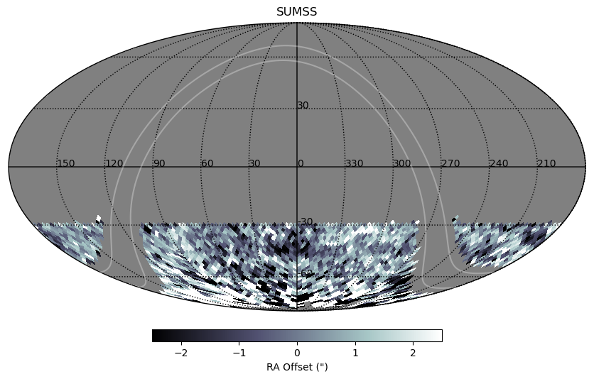
(a) SUMSS

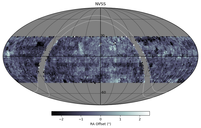
(b) NVSS

Figure 12: Comparison of the median RA offsets, for each HEALPix bin, between RACS and SUMSS (left) and NVSS (right) for sources matched with the criteria in Section 5.2.2 as a function of position across the sky.

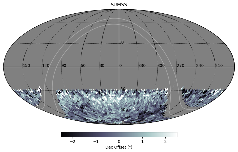
(a) SUMSS

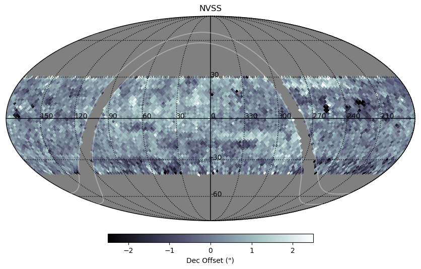
(b) NVSS

Figure 13: Comparison of the median Dec offsets, for each HEALPix bin, between RACS and SUMSS (left) and NVSS (right) for sources matched with the criteria in Section 5.2.2 as a function of position across the sky.

5.2.5 Spectral Index Comparisons

Finally, we compare the spectral index between RACS and radio surveys at other frequencies, assuming a power law spectral energy distribution (SED) as discussed in Section 5.2.2. We define $\alpha$ here as:

$$\alpha^{\textrm{RACS}}_{\textrm{Comp}}=\frac{\log\left(\frac{S_{\textrm{RACS}}}{S_{\textrm{Comp}}}\right)}{\log\left(\frac{\nu_{\textrm{RACS}}}{\nu_{\textrm{Comp}}}\right)}.$$ (2)

It is important when measuring the spectral indices between matched catalogues that the sensitivity limits are considered. This will bias spectral indices to either lower or higher values depending on the sensitivity limits and frequencies of the comparison surveys. Therefore we consider the spectral index for our matched sources both with and without a flux density cut applied. To determine the flux density cuts to apply we assume the sensitivity limits of each survey to be the 5$\sigma$ sensitivity limits in Table 4 or the approximate 10$\sigma$ sensitivity of RACS (taken here as 3 mJy). Using these sensitivity limits, we determine the flux density cuts that are necessary to ensure there is no bias within the range $\alpha=-0.8\pm 1.2$, which should encompass the majority of $\alpha$ values observed (see e.g. Smolčić et al., 2017a; Tiwari, 2019). We then apply any necessary flux cuts to avoid any bias in $\alpha$. This flux density cut greatly reduces the number of sources available for comparisons. The histogram distribution of these spectral indices can be seen in Figure 14 (left) as well as the comparison of spectral index with flux density (right). This latter plot indicates the necessity of applying a flux limit cut when investigating the spectral index.

For spectral index comparisons, we do not consider $\alpha^{\rm RACS}_{\rm SUMSS}$ due to the small frequency offset. However we add in a comparison to the rescaled TGSS-ADR catalogue from Hurley-Walker (2017). This adjusted the flux scale of TGSS-ADR based on measurements from the GLEAM survey. For comparisons to this survey we will use the label ‘TGSS-ADR-R’.

From Figure 14 we find a typical median $\alpha$ in the range $\sim-$0.6 to $-$0.9, encompassing the typical values expected of $\sim-$0.7 to $-$0.8. Without a flux cut applied, the median $\alpha$ and errors from the 16^th and 84^th percentiles are measured as: $-0.69^{+0.25}_{-0.21}$ (GLEAM), $-0.87^{+0.52}_{-0.42}$ (NVSS), $-0.64^{+0.26}_{-0.23}$ (TGSS-ADR) and $-0.62^{+0.25}_{-0.22}$ (TGSS-ADR-R). When a flux cut is applied, these are now measured as: $-0.61^{+0.32}_{-0.19}$ (GLEAM), $-0.90^{+0.43}_{-0.39}$ (NVSS), $-0.59^{+0.36}_{-0.22}$ (TGSS-ADR) and $-0.58^{+0.36}_{-0.21}$ (TGSS-ADR-R). The comparisons with the low frequency surveys of TGSS-ADR and GLEAM are closer to $-$0.6 to $-$0.7 whilst the higher frequency comparison with NVSS is more similar to $-$0.9. This may suggest that the RACS fluxes are slightly larger than expected from previous surveys, however as shown in Section 5.2.3 we have a good flux comparison with SUMSS.

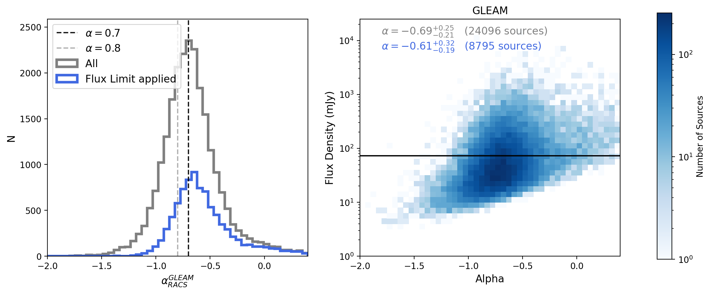
(a) GLEAM

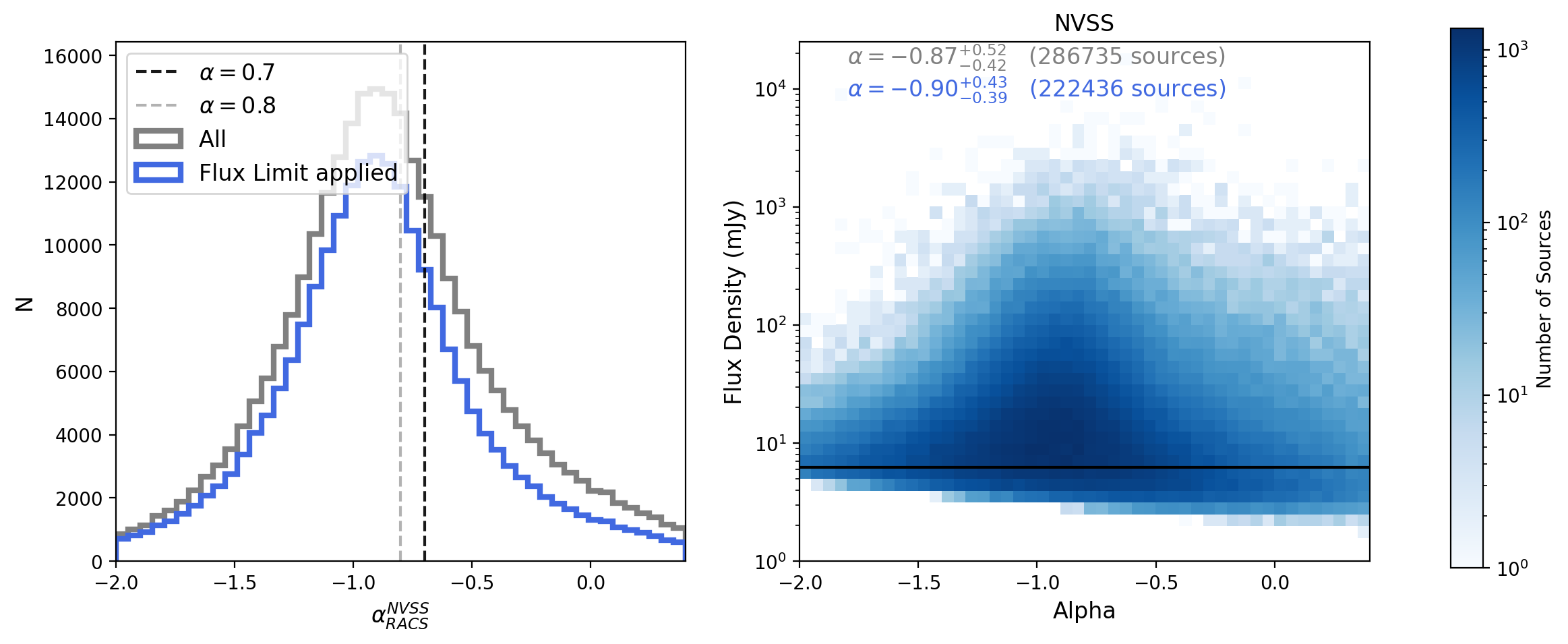
(b) NVSS

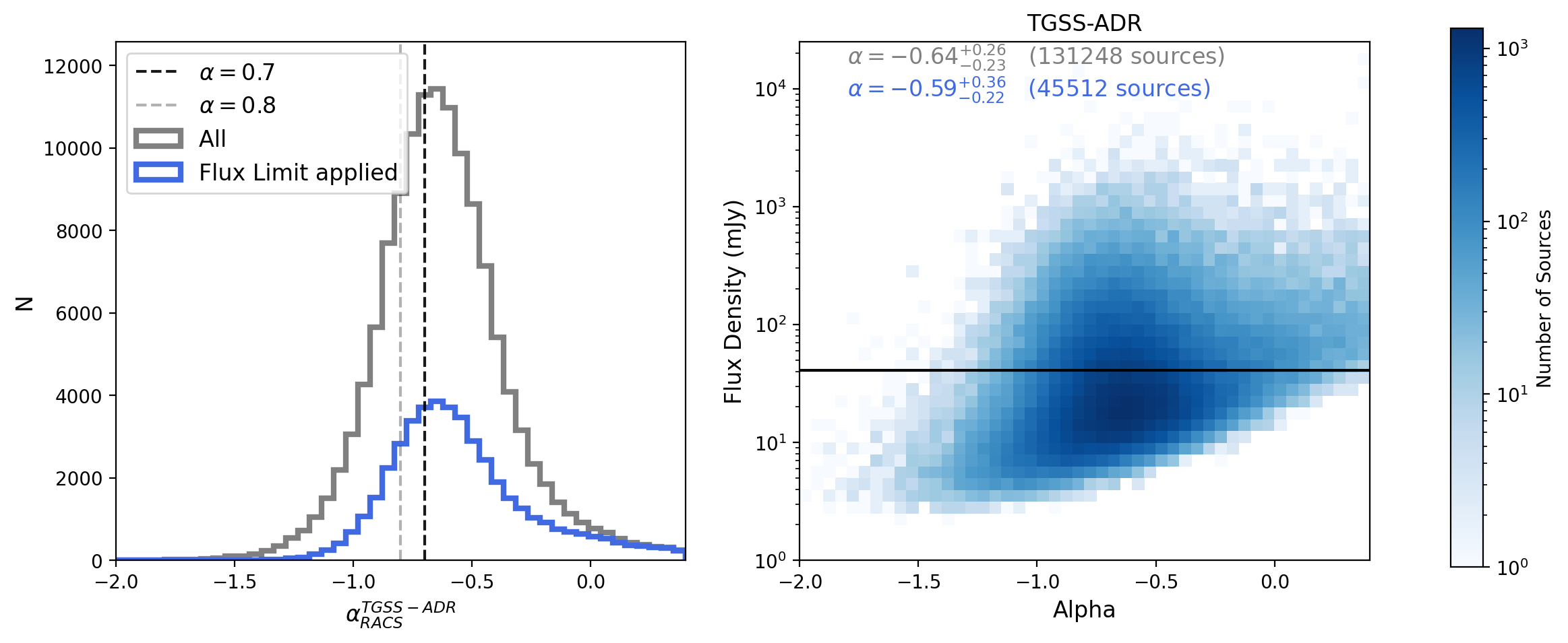
(c) TGSS-ADR

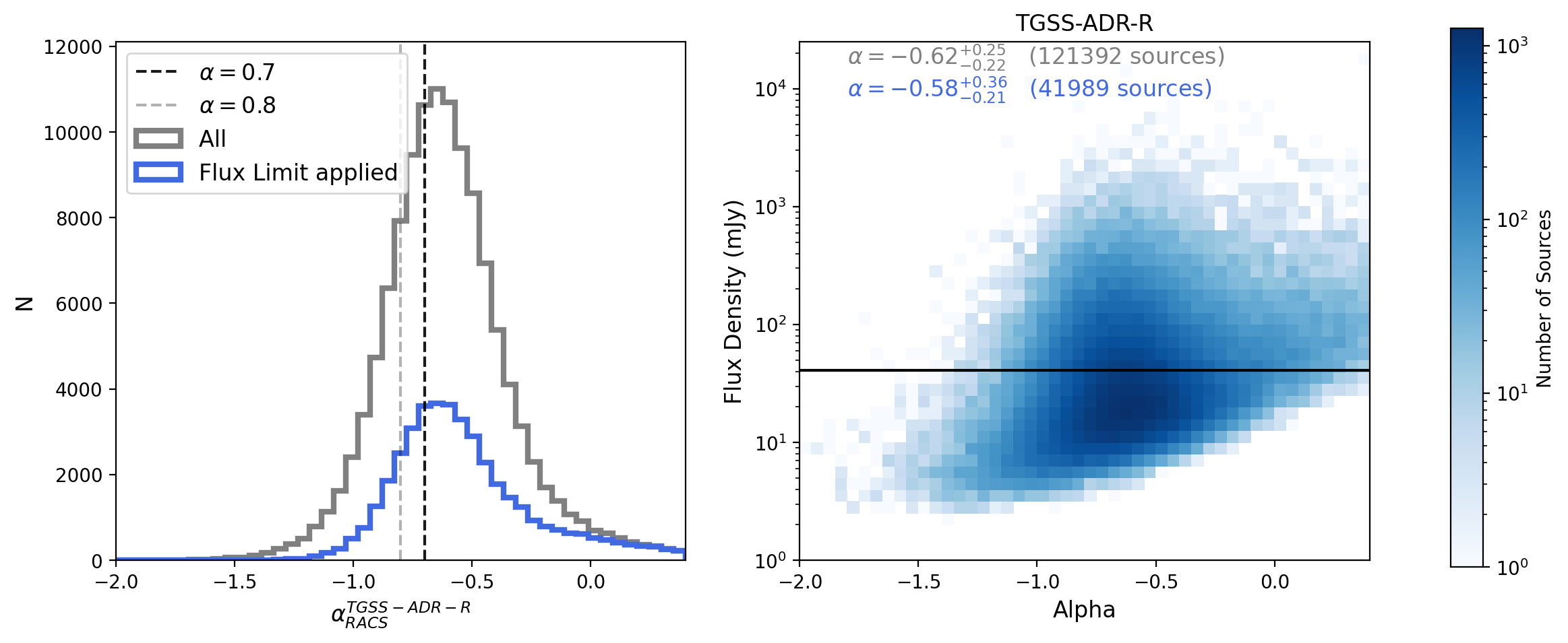
(d) TGSS-ADR-R

Figure 14: Comparison of the spectral indices between RACS and (a) GLEAM, (b) NVSS, (c) TGSS-ADR and (d) the Rescaled TGSS-ADR catalogue. For each panel, the left panel shows the histogram distribution of $\alpha$, whilst the right panel shows the distribution of $\alpha$ with flux density. This is shown with (blue) and without (grey) a flux cut (see Section 5.2.5). A black solid line indicates where the flux density cut is applied.

In general, these comparisons have shown that we have good systematic astrometric and flux characteristics compared to other surveys. Measurements of the spectral indices of RACS sources will also be improved with future RACS observations, which are planned for different frequency bands (see Paper I).

6 Completeness

We consider the completeness of our catalogue as a function of flux density. It should be close to unity at high flux densities and will decline towards zero close to the detection threshold of the survey. Completeness is affected by both the variation of rms across the survey area, which affects the detection threshold, as well as the source finder itself. We therefore need to consider the completeness of this catalogue as a function of flux density.

We consider the survey completeness in two forms, for unresolved sources and for a combination of both unresolved (point) and resolved sources. To investigate both of these, we use simulations in which we inject sources into the residual images (Image - Model from PyBDSF) and investigate the recovery of the injected sources with PyBDSF. These simulations are described below.

6.1 Point Source Detection

First, to investigate the point source completeness, we injected Gaussians with the resolution of the images i.e. a circular PSF of 25^′′ FWHM into our residual images. To consider the detection of sources at a variety of realistic radio flux densities, we use the simulated catalogues from SKADS (Wilman et al., 2008; Wilman et al., 2010). These simulations were created in preparation for the Square Kilometre Array (SKA) to provide realistic mock catalogues that reflect both observations from existing radio surveys as well as expectations of radio sources below current sensitivity limits.

For 5 million random positions across the range $\delta=-$85^∘ to +30^∘ we find the closest tile for each random source. For each tile we consider the random sources which are closest to that tile and for each source we randomly choose a flux density from SKADS and scale this from 1400 MHz to 887.5 MHz, assuming a spectral index of $\alpha=-0.8$. We inject a Gaussian component with the simulated total flux density into the residual image at the random position generated. PyBDSF is then used to investigate the detection of simulated sources within the image, using the same parameters as in Section 3. From this the comparison of detected sources across the image can be calculated. We repeat this for each tile within the observation. We repeat this method 10 times to make multiple realisations of the simulated distribution of sources. We estimate the average completeness from the mean completeness in each flux bin considered and the error from the standard deviation across the 10 realisations.

Once all the output PyBDSF catalogues have been calculated for each field and for each simulation realisation, we compare the input sources to those measured. For each field, we match the input catalogue to the recovered catalogue and class those sources as “recovered" as those output source which match to an input source within half the FWHM resolution of our images (i.e. 12.5 ^′′). We then calculate the detection fraction in two methods.

First within each flux density bin, we investigate the fraction of sources that have a “recovered" counterpart. The result of this can be seen in the left panel of Figure 15. This shows approximately 50% detection at $\sim$1.7 mJy and 95% detection at $\sim 5.0$ mJy. From this, we also consider the overall completeness of the sources detected in the survey. To do this, we combine knowledge of the underlying flux distribution of sources from the SKADS simulations, with the fraction that are detected. For each flux density bin (logarithmically sampled) we sum the product of the detection fraction with the input source count distribution from the random sources at flux densities greater than or equal to the flux density bin being considered. This is normalised to the sum of the full input source count distribution. This overall completeness can be seen in the left hand of Figure 15. This suggests an overall 50% completeness at $\sim$0.8 mJy and 95% completeness at $\sim 2.9$ mJy.

Secondly we consider the effect of flux measurement by the source finder and how this may affect the apparent distribution of fluxes. This comparison of input to measured flux distribution can be seen in Figure 16 (left panel for point sources). As can be seen, these measured fluxes are scattered around the 1-to-1 measurement line (black line), but will have a positive bias, especially at fainter flux densities. This positive bias is a combination of the effect of the measurement of source fluxes being affected by noise peaks/trough a source is on and, as brighter sources are more likely to be detected, sources which lie on a positive noise spike are more likely to be detected. Moreover, as there are more faint sources within the simulations, these are more likely to be affected by this positive bias.

To determine the point source detection fraction, with this second method, we compare the binned distribution of flux densities recovered by PyBDSF compared to the input flux density distribution of the simulated sources injected into the image. The ratio of the output flux density distribution compared to the input flux density distribution is therefore a measurement of the detection fraction of point sources across the image. This can be seen as the black line in the right panel of Figure 15. As the change in flux density can be seen through this measurement, it is possible to have detection fractions larger than one. This will reflect that, due to differences between input and output flux densities, there are more sources observed in a flux density bin than were input into the simulation. This method suggests a completeness of 50% for point sources with a flux density of $\sim$1.8 mJy and 95% at a flux density $\sim 2.7$ mJy. This method will be especially important in the discussion of source counts in Section 7.

For both methods though, we determine the average detection fraction and completeness in each flux density bin by the mean value from the simulations. The associated error is then taken as the standard deviation from the simulation realisations.

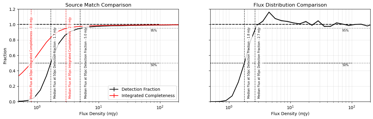
Figure 15: Detection fraction and completeness as a function of flux density for point source simulations. Left: Detection fraction and total catalogue completeness for sources which are matched based on positional location alone. The vertical lines indicate the 50% and 95% detection fraction levels (black; at 1.7 mJy and 5.0 mJy) and 50% and 95% completeness (red; at 0.8 mJy and 2.9 mJy). Right: Detection fraction of sources as a function of flux density based on comparing the input to measured flux density distribution (50% at 1.8 mJy and 95% at 2.7 mJy).

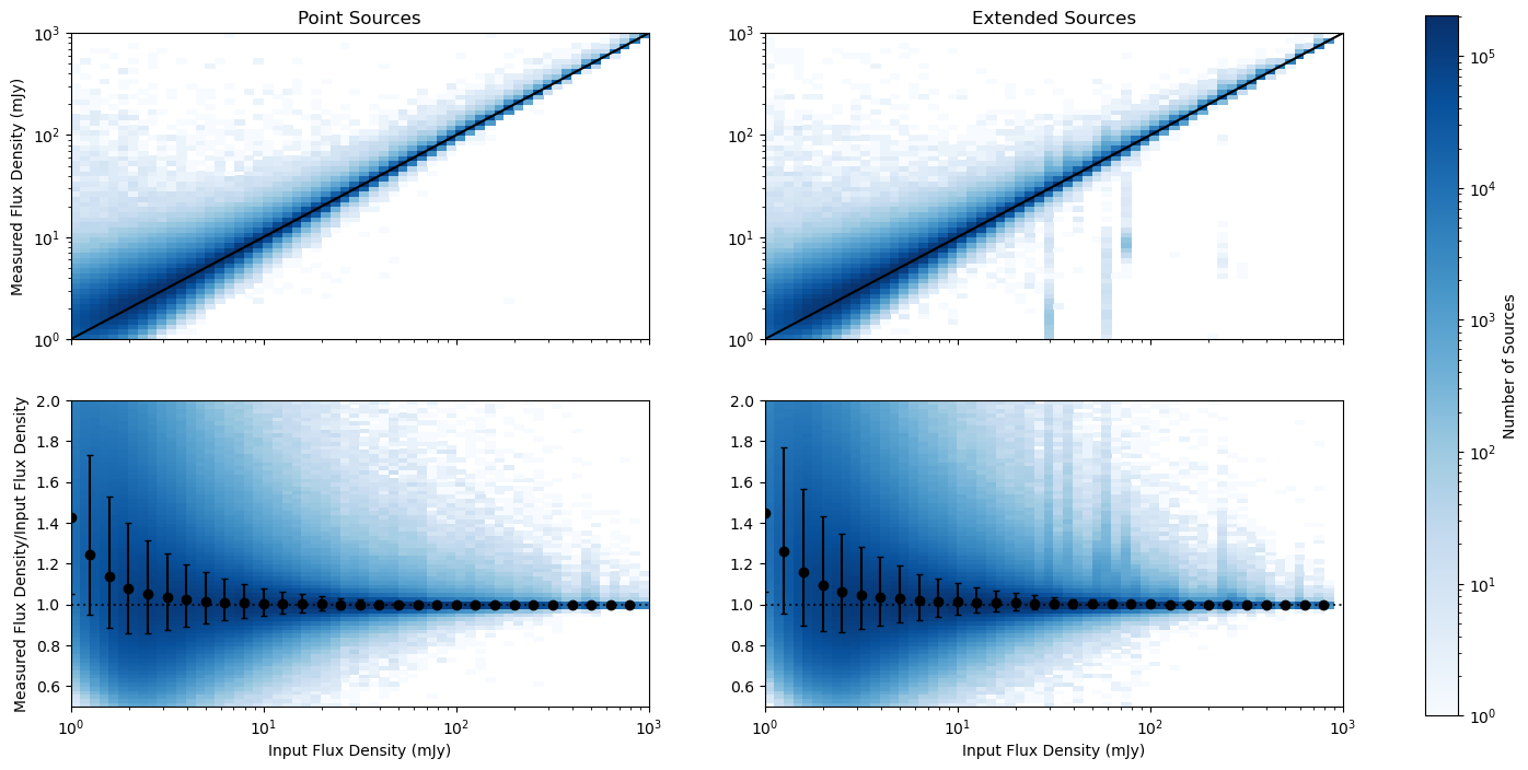
Figure 16: Comparison of input to measured fluxes for simulated sources in the (left) point source simulations and (right) resolved source simulations. Upper panels show the comparison of input and measured fluxes and lower panels show the median measured to input flux ratio as a function of input flux density. The black points indicate the median flux ratio within the bin and the errors are calculated from the 16${}^{\textrm{th}}$ and 84${}^{\textrm{th}}$ percentiles.

6.2 Resolved Source Completeness

Next we investigate the effect of source size on completeness, as the previous section neglects the effect of resolution bias. Resolution bias accounts for the relative difficulty in detecting extended sources compared to point sources. An extended source with the same integrated flux density as a point source will have a lower peak flux density, an effect that becomes more important at low SNR. This will be important to consider as the majority of sources in this catalogue are believed to be resolved (see Figure 8).

To investigate this, we again use the simulated sources from Wilman et al. (2008); Wilman et al. (2010), using the source size models associated with each source. SKADS sources are described by a single or a combination of components which are described by ellipses. This will therefore contain a combination of single-component sources for objects such as SFGs as well as multi-component lobed FRI and FRII sources. These simulations should therefore give a more realistic distribution of the diverse ranges of sources expected within radio surveys and will contain a combination of resolved and unresolved sources.

To consider the completeness of a realistic distribution of resolved and unresolved sources, we follow the same method as in Section 6.1 however, first convolving the ellipse source model with the Gaussian PSF, ensuring the flux scale is retained. After running PyBDSF on each image, we use the same process as in Section 6.1 to compare the input and output catalogues and determine the detection fraction. This detection fraction is shown in Figure 17 and the comparison of input to measured flux densities can be seen in the right hand panel of Figure 16. This shows that 50% of sources at $\sim$1.8 (1.9) mJy will be detected, increasing to a 95% detection fraction at approximately $\sim$8.6 (3.3) mJy using method 1 (2) described above. This indicates a poorer detection fraction than for point sources, reflecting the effect of resolution bias on the detection of sources. However, it could also relate to the fact that the simulated sources are extended and made of multiple components and so matching using a positional radius may lead to errors in matching components to a single source and so larger errors between the positional location of the input to measured source. Issues due to this would also be seen in flux density comparisons in Figure 16 where the input and measured flux densities appear offset.. Computing the overall completeness of our catalogue from method 1 suggests 50% completeness at $\sim$0.9 mJy and 95% completeness at $\sim$4.7 mJy.

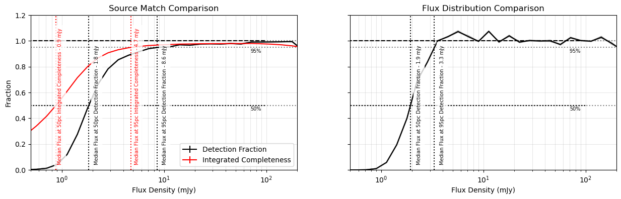
Figure 17: Detection fraction and completeness as a function of flux density for the resolved source simulations. Left: Detection fraction and total catalogue completeness for sources which are matched based on positional location alone. The vertical lines indicate the 50% and 95% detection fraction levels (black; at 1.8 mJy and 8.6 mJy) and 50% and 95% completeness (red; at 0.9 mJy and 4.7 mJy). Right: Detection fraction of sources as a function of flux density based on comparing the input to measured flux density distribution (50% at 1.9 mJy and 95% at 3.3 mJy).

6.3 Limitations of the Simulations

We identify three separate limitations to the simulations we have used to analyse the survey completeness. First, these simulations inject sources into the residual image. Therefore these will not account for any issues that are introduced through the calibration pipeline or any effects of CLEAN bias (see e.g. Section 7.2 of Becker et al., 1995) or time and bandwidth smearing (see e.g. Bridle & Schwab, 1989). Furthermore, some smearing may occur where images are mosaiced together which could affect source detectability, this includes both when beams are mosaiced together to form a tile and where tiles are mosaiced with other neighbouring tiles. To improve this, sources could be injected into the visibilities and processed through the pipeline, however for 799 tiles, this is an arduous process.

Second, these simulations will be affected if the source morphologies assumed in SKADS and flux density distribution of input sources are not as accurate a representation of the underlying source distribution as expected. This may also be the case if the morphologies observed with ASKAP are more susceptible to extended emission and complex morphologies which may not be well modelled in SKADS using elliptical components. In term of flux density distribution, though, the source counts from Wilman et al. (2008) seem to well recreate observations at the flux densities probed by RACS. This may, however, not be the case at fainter fluxes (see e.g. Smolčić et al., 2017a; Mauch et al., 2020; Matthews et al., 2021).

Finally, these simulations may not properly account for the effect of having multiple sources located in close proximity to each other. This is as the sources are injected at random positions and so will have a uniform source density. This will not account for the clustering of real sources due to the large scale structure of the Universe. Moreover, in the matching process there may be issues arising from simulated sources merging into a single source if they are located in close proximity. This could affect whether input to output simulated sources are matched together as well as any input to output flux ratios.

Despite these limitations, these simulations should give a good understanding of how well we are detecting realistic radio sources within our images. We shall discuss further how successful these simulations appear to be, given their effect on the measured source counts, in Section 7.

6.4 Reliability

Next we assess the reliability of these observations following the approach of Intema et al. (2017). This considers the contamination of noise within the catalogue by considering the source detection over the negative image (i.e. $-$1 $\times$ image). The technique relies on the premise that the noise in the image is symmetric. Therefore running PyBDSF over the negative images using the same parameters as in Section 3 can indicate the distribution of positive noise which may have contaminated the final source catalogue.

We concatenate the PyBDSF catalogues from the negative images in the same way as described in Section 3, to avoid source duplication. The distribution of source flux densities from the negative image compared to the final catalogues is shown in Figure 18. The number of negative sources is small compared to real sources within the catalogue ($\sim 0.3$%), suggesting that the number of false detections within the final source catalogue is negligible compared to real sources.

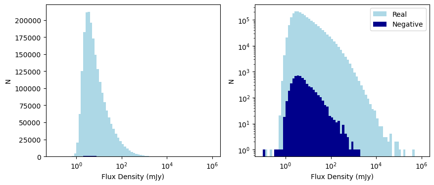
Figure 18: Comparison of the flux density distribution of sources detected in the negative image (dark blue) compared to the full survey catalogue (light blue). This is shown with both a linear (left) and logarithmic (right) scaled y-axis.

6.5 Density as function of declination

Finally, in order to consider the completeness as a function of sky position we present the variation of source density of the catalogue with declination. This is shown in Figure 19 for all sources in the source catalogue, where we have excluded the Galactic plane. The density of sources with a total flux density above or equal to the six different flux density limits quoted (1, 2, 3, 4, 5 and 10 mJy) is shown. In Figure 19, the left hand panel shows this source density as a function of declination, whilst the right hand panel indicates the area which is being considered whilst constructing the source density. The integrated total number density of sources above a given flux density is presented in Table 5.

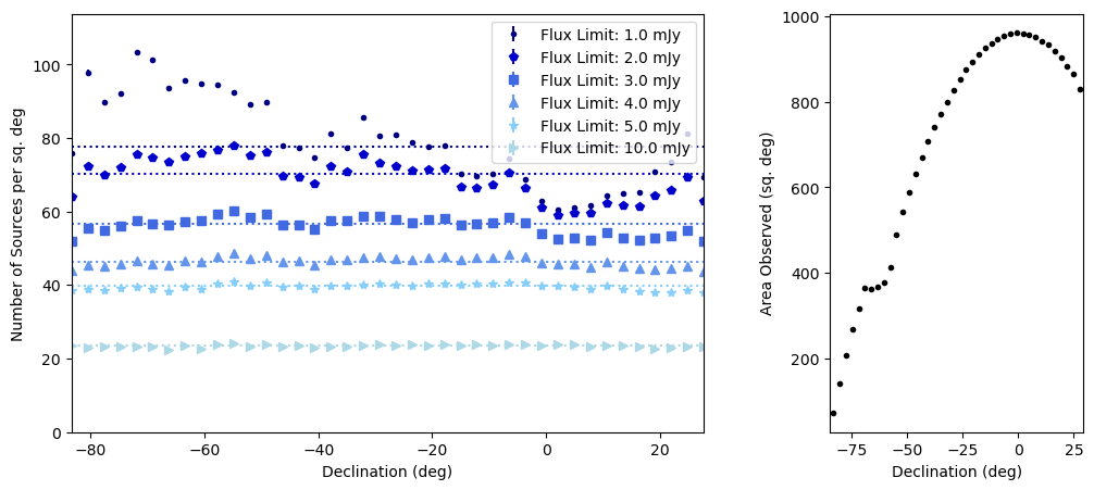
Figure 19: Left: Source density as a function of Declination for those sources with total flux densities above six limits. This is shown for the whole catalogue but with regions around the Galactic plane ($|b|<5$^∘) removed. Right: The corresponding sky area observed as a function of declination for the catalogue excluding the Galactic plane.

$S$	N ($>S$)	N ($>S$)
(mJy)	($\rm{sr}^{-1}$)	($\rm{deg}^{-2}$)
0.5	249000.0	75.8
1.0	248000.0	75.6
2.0	224000.0	68.1
3.0	183000.0	55.9
5.0	130000.0	39.6
10.0	77100.0	23.5
20.0	43900.0	13.4
50.0	19100.0	5.8
100.0	9240.0	2.8
200.0	3980.0	1.2

Table 5: The integrated source counts of sources in the first RACS Stokes I catalogue above quoted flux density limits. We note that in the faintest flux density bins, the integral source counts will be affected by incompleteness (see Section 6).

As can be seen in Figure 19, the source density within our catalogue is approximately flat across the entire declination range observed for flux density limits $\geq 4$ mJy. In the 1 and 2 mJy flux density limit bins, on the other hand, the incompleteness limits within the data means that the source density is more variable over the declination range. These are still relatively small variations at 3 mJy; however, for the 1 mJy limit, the source density of sources around $\delta=-$60^∘ is much larger compared to at other declination ranges. Moreover, due to the higher rms that can be seen in Figure 5, there is an under-density in sources at declinations of $\sim$0^∘ to +20^∘ in both the 1 and 2 mJy bins.

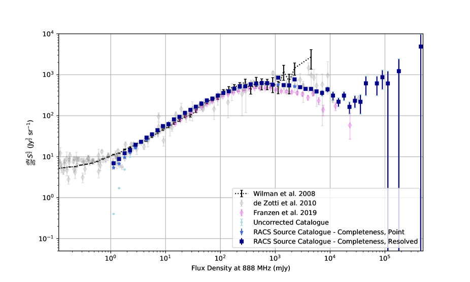
Figure 20: Comparison between the Euclidean normalised source counts from this catalogue and previous surveys and simulations. Presented are the source counts from de Zotti et al. (2010) (grey diamonds), Franzen et al. (2019) (magenta diamonds) and the SKADS catalogue from Wilman et al. (2008); Wilman et al. (2010) (black line). For our catalogue, we present the raw source counts (light blue) as well as those corrected using the point source detection fraction in Section 6.1 (blue) and those using the variable size detection fraction from Section 6.2 (dark blue). The RACS number counts cover an area of 28,020 deg². All surveys not at 887.5 MHz have been converted to this frequency assuming $\alpha=-0.8$.

7 Source Counts

Finally, using our finished catalogue and, having quantified the completeness within our sample, we compare the source count distribution of the radio sources identified in our catalogue to previous surveys. Whilst narrow, deep surveys help to fill in the source count distribution of faint sources, it is only with large area surveys that the source count distribution of the brightest sources can be understood. This is because these bright objects are rare. Source counts describe the number of sources within a given flux density bin per steradian on the sky. These are typically normalised by multiplying by $S^{2.5}$ (where $S$ is the total flux density) to define the Euclidean normalised source counts (see e.g. Heywood et al., 2013, for an explanation).

Radio source counts are constructed for most radio survey catalogues (see e.g. Bondi et al., 2008; Smolčić et al., 2017a; Shimwell et al., 2019) and so compilations of the source counts from multiple surveys exist (e.g. de Zotti et al., 2010). We therefore determine the source counts for our catalogue and make comparisons to the past survey source counts compiled by de Zotti et al. (2010) and the low frequency source counts from GLEAM from Franzen et al. (2019), which cover large sky areas, in Figure 20. Here we illustrate the source count distribution for the source catalogue discussed in Section 3. The raw count from this catalogue can be seen as the light blue circles in Figure 20.

However, as discussed in Section 6, our observations are not complete to the faintest flux density limits to which we observe. This is due to the fact that there are noise variations across the full survey area of RACS, meaning that the faintest sources are unable to be detected uniformly. To make a correction for this and to correct the measured source counts to what would be observed if the rms was uniform, we make use of the detection fraction curves described in Section 6. Specifically, we use the detection fraction where we account for variations in flux density (see Figures 15 and 17 - right). We use this as the measurements of the flux densities of sources will also be affected by any differences between the true and measured source densities.

Using the detection fraction as a function of flux density, we corrected the raw counts using the detection fractions from Sections 6.1 and 6.2 to understand the intrinsic source count distribution. We calculated the associated errors by adding in quadrature the errors from both the poisson statistics of the data itself, with the errors from the completeness simulations (see Section 6.1). In Figure 20, we plot the source counts only for those sources that have a flux density (at 887.5 MHz) of greater than 1 mJy. These are compared to the compilation of measured source counts from de Zotti et al. (2010) as well as the source counts from the extra-galactic simulated catalogues of SKADS (both converted to 887.5 MHz assuming $\alpha=-$0.8). We apply corrections based on both the point source only corrected simulations (Section 6.1; blue) as well as the simulations which have both point and extended simulated sources (Section 6.2; dark blue). These are both plotted so that the effect of source size can be investigated.

As can be seen from Figure 20, these corrections only affect the lowest flux density bins, below approximately 5 mJy. Using the corrections from Section 6 we find that if we only include point sources in our investigations, then the source counts appear too small at faint flux densities in comparison to previous observations. When the effect of extended sources is included, these source counts are further corrected and are now in much better agreement with the source counts from de Zotti et al. (2010) and Wilman et al. (2008). However, these source counts may still possibly appear too low in the faintest flux density bins and possible explanations for this can be found in Section 6.3. A table of the resulting RACS source counts can be found in Table 6.

At high flux densities, we find that RACS is able to provide tight constraints on the source counts, due to the large area coverage of the survey. Importantly, this allows the source counts at flux densities at values $\gtrsim$ 10⁴ mJy that are not well investigated in the de Zotti et al. (2010) compilation catalogue to be seen. The source counts presented at these high flux densities do appear higher than the counts from Franzen et al. (2019). This may reflect differences in the source populations observed at lower frequencies (200 MHz).

$S$	$S_{mid}$	N	Raw $\frac{dN}{dS}S^{2.5}$	Corrected $\frac{dN}{dS}S^{2.5}$	Corrected $\frac{dN}{dS}S^{2.5}$
				(Point)	(Resolved)
(mJy)	(mJy)		(Jy1.5sr-1)	(Jy1.5sr-1)	(Jy1.5sr-1)
1.00 - 1.26	1.13	20653 $\pm$ 143	0.40 $\pm$ 0.01	5.41 $\pm$ 0.04	6.91 $\pm$ 0.05
1.26 - 1.58	1.42	62252 $\pm$ 249	1.71 $\pm$ 0.01	6.77 $\pm$ 0.03	8.76 $\pm$ 0.03
1.58 - 2.00	1.79	125409 $\pm$ 354	4.85 $\pm$ 0.01	9.67 $\pm$ 0.04	12.14 $\pm$ 0.05
2.00 - 2.51	2.25	182302 $\pm$ 426	9.97 $\pm$ 0.02	12.64 $\pm$ 0.05	14.42 $\pm$ 0.04
2.51 - 3.16	2.84	211331 $\pm$ 459	16.32 $\pm$ 0.04	16.52 $\pm$ 0.05	19.52 $\pm$ 0.05
3.16 - 3.98	3.57	212212 $\pm$ 460	23.15 $\pm$ 0.05	22.20 $\pm$ 0.08	23.13 $\pm$ 0.06
3.98 - 5.01	4.50	196155 $\pm$ 442	30.22 $\pm$ 0.07	26.05 $\pm$ 0.07	29.26 $\pm$ 0.08
5.01 - 6.31	5.66	172900 $\pm$ 415	37.63 $\pm$ 0.09	34.93 $\pm$ 0.11	35.08 $\pm$ 0.16
6.31 - 7.94	7.13	149416 $\pm$ 386	45.93 $\pm$ 0.12	43.76 $\pm$ 0.18	44.42 $\pm$ 0.20
7.94 - 10.00	8.97	127989 $\pm$ 357	55.58 $\pm$ 0.16	53.50 $\pm$ 0.22	55.76 $\pm$ 0.17
10.00 - 12.59	11.29	109141 $\pm$ 330	66.94 $\pm$ 0.20	65.61 $\pm$ 0.23	62.32 $\pm$ 0.26
12.59 - 15.85	14.22	93233 $\pm$ 305	80.78 $\pm$ 0.26	80.08 $\pm$ 0.29	81.44 $\pm$ 0.35
15.85 - 19.95	17.90	79828 $\pm$ 282	97.69 $\pm$ 0.35	94.11 $\pm$ 0.48	93.96 $\pm$ 0.47
19.95 - 25.12	22.54	67405 $\pm$ 259	116.52 $\pm$ 0.45	117.65 $\pm$ 0.62	117.59 $\pm$ 0.64
25.12 - 31.62	28.37	57111 $\pm$ 238	139.46 $\pm$ 0.58	133.16 $\pm$ 0.67	139.05 $\pm$ 0.64
31.62 - 39.81	35.72	48027 $\pm$ 219	165.65 $\pm$ 0.76	169.85 $\pm$ 0.97	165.73 $\pm$ 0.88
39.81 - 50.12	44.96	40703 $\pm$ 201	198.31 $\pm$ 0.98	203.36 $\pm$ 1.16	198.17 $\pm$ 1.26
50.12 - 63.10	56.61	33434 $\pm$ 182	230.09 $\pm$ 1.25	225.41 $\pm$ 1.41	236.64 $\pm$ 1.41
63.10 - 79.43	71.26	27623 $\pm$ 166	268.53 $\pm$ 1.61	267.23 $\pm$ 1.66	261.96 $\pm$ 1.78
79.43 - 100.00	89.72	22715 $\pm$ 150	311.91 $\pm$ 2.06	316.13 $\pm$ 2.20	311.06 $\pm$ 2.15
100.00 - 125.89	112.95	18415 $\pm$ 135	357.18 $\pm$ 2.62	356.92 $\pm$ 2.71	357.94 $\pm$ 2.72
125.89 - 158.49	142.19	14763 $\pm$ 121	404.47 $\pm$ 3.32	402.96 $\pm$ 3.45	393.35 $\pm$ 3.84
158.49 - 199.53	179.01	11648 $\pm$ 107	450.78 $\pm$ 4.14	459.76 $\pm$ 4.28	458.81 $\pm$ 4.72
199.53 - 251.19	225.36	8908 $\pm$ 94	486.96 $\pm$ 5.14	483.41 $\pm$ 5.16	523.56 $\pm$ 5.45
251.19 - 316.23	283.71	6898 $\pm$ 83	532.64 $\pm$ 6.41	533.12 $\pm$ 6.49	522.06 $\pm$ 6.85
316.23 - 398.11	357.17	5228 $\pm$ 72	570.23 $\pm$ 7.85	580.13 $\pm$ 8.44	584.12 $\pm$ 8.72
398.11 - 501.19	449.65	3815 $\pm$ 61	587.77 $\pm$ 9.40	581.66 $\pm$ 9.40	610.97 $\pm$ 11.54
501.19 - 630.96	566.07	2859 $\pm$ 53	622.20 $\pm$ 11.53	606.49 $\pm$ 11.46	629.78 $\pm$ 11.46
630.96 - 794.33	712.64	2047 $\pm$ 45	629.26 $\pm$ 13.83	631.10 $\pm$ 13.97	622.63 $\pm$ 14.46
794.33 - 1000.00	897.16	1389 $\pm$ 37	603.14 $\pm$ 16.07	600.81 $\pm$ 16.14	572.48 $\pm$ 17.90
1000.00 - 1258.93	1129.46	931 $\pm$ 30	571.04 $\pm$ 18.40	574.04 $\pm$ 18.62	850.87 $\pm$ 21.91
1258.93 - 1584.89	1421.91	644 $\pm$ 25	557.96 $\pm$ 21.66	556.81 $\pm$ 21.65	559.08 $\pm$ 21.70
1584.89 - 1995.26	1790.08	448 $\pm$ 21	548.27 $\pm$ 25.70	547.25 $\pm$ 25.70	549.16 $\pm$ 25.69
1995.26 - 2511.89	2253.57	300 $\pm$ 17	518.60 $\pm$ 29.39	518.29 $\pm$ 29.39	768.21 $\pm$ 31.82
2511.89 - 3162.28	2837.08	205 $\pm$ 14	500.57 $\pm$ 34.19	500.57 $\pm$ 34.19	497.07 $\pm$ 34.41
3162.28 - 3981.07	3571.67	131 $\pm$ 11	451.84 $\pm$ 37.94	452.25 $\pm$ 38.00	451.84 $\pm$ 37.98
3981.07 - 5011.87	4496.47	92 $\pm$ 9	448.23 $\pm$ 43.85	450.67 $\pm$ 44.12	450.99 $\pm$ 44.16
5011.87 - 6309.57	5660.72	57 $\pm$ 7	392.27 $\pm$ 48.17	387.84 $\pm$ 47.71	392.27 $\pm$ 47.63
6309.57 - 7943.28	7126.43	37 $\pm$ 6	359.68 $\pm$ 58.33	359.68 $\pm$ 58.33	359.68 $\pm$ 58.33
7943.28 - 10000.00	8971.64	32 $\pm$ 5	439.40 $\pm$ 68.66	439.40 $\pm$ 68.66	439.40 $\pm$ 68.66
10000.00 - 12589.25	11294.63	16 $\pm$ 4	310.34 $\pm$ 77.58	310.34 $\pm$ 77.58	310.34 $\pm$ 77.58
12589.25 - 15848.93	14219.09	8 $\pm$ 2	219.18 $\pm$ 54.80	219.18 $\pm$ 54.80	219.18 $\pm$ 54.80
15848.93 - 19952.62	17900.78	8 $\pm$ 2	309.60 $\pm$ 77.40	309.60 $\pm$ 77.40	309.60 $\pm$ 77.40
19952.62 - 25118.86	22535.74	3 $\pm$ 1	164.00 $\pm$ 54.67	164.00 $\pm$ 54.67	164.00 $\pm$ 54.67
25118.86 - 31622.78	28370.82	3 $\pm$ 1	231.65 $\pm$ 77.22	231.65 $\pm$ 77.22	231.65 $\pm$ 77.22
31622.78 - 39810.72	35716.75	2 $\pm$ 1	218.14 $\pm$ 109.07	218.14 $\pm$ 109.07	218.14 $\pm$ 109.07
39810.72 - 50118.72	44964.72	4 $\pm$ 2	616.27 $\pm$ 308.14	616.27 $\pm$ 308.14	616.27 $\pm$ 308.14
63095.73 - 79432.82	71264.28	2 $\pm$ 1	614.82 $\pm$ 307.41	614.82 $\pm$ 307.41	614.82 $\pm$ 307.41
79432.82 - 100000.00	89716.41	2 $\pm$ 1	868.45 $\pm$ 434.22	868.45 $\pm$ 434.22	868.45 $\pm$ 434.22
100000.00 - 125892.54	112946.27	1 $\pm$ 1	613.36 $\pm$ 613.36	613.36 $\pm$ 613.36	613.36 $\pm$ 613.36
158489.32 - 199526.23	179007.78	1 $\pm$ 1	1223.81 $\pm$ 1223.81	1223.81 $\pm$ 1223.81	1223.81 $\pm$ 1223.81
398107.17 - 501187.23	449647.20	1 $\pm$ 1	4872.08 $\pm$ 4872.08	4872.08 $\pm$ 4872.08	4872.08 $\pm$ 4872.08

Table 6: Table of source counts at 887.5 MHz accompanying Figure  20. The raw and the corrected source counts using the corrections for point (Section 6.1) and resolved (Section 6.2) are quoted. A total sky area of 28,020 deg² was used.

8 Conclusions

In this paper we have presented the first Stokes I catalogue release for the Rapid ASKAP Continuum Survey (RACS, McConnell et al., 2020). This first catalogue contains the majority of the Southern sky in the Declination region $-$80^∘ to +30^∘ using 799 tiles across the sky. These observations were reduced as described in McConnell et al. (2020) and in this paper we describe the process of mosaicing the observations together and producing a single source catalogue. We present the source catalogue of 2,123,638  islands and 2,462,693  components which were derived from PyBDSF catalogues over each of the 799 tiles. These have been combined together to form a full catalogue which removes duplicate sources. This catalogue will be released for download from CASDA (Chapman et al., 2017; Huynh et al., 2020) with the publication of the paper.

For quality assessment, we have compared the results of this work to previous large sky radio surveys from GLEAM, NVSS, SUMSS and TGSS-ADR. This has allowed quantification of the accuracy in the flux density scale and astrometry, along with the spectral indices implied from our data. We find good flux density agreement with SUMSS, finding a RACS-to-SUMSS flux density ratio of $1.00^{+0.16}_{-0.16}$. Our median astrometric offsets from comparisons with SUMSS and NVSS appear to be limited to a pixel (2.5^′′) with most offsets constrained to less than two pixels. Finally, we find typical $\alpha$ measurements of $\sim-$0.6 compared to radio observations at lower frequency to RACS and $\sim-$0.9 for surveys at higher frequencies.

We have further analysed the data using simulations to investigate the detection fraction of both point and resolved sources within our images as a function of flux density. Using these measurements, we determined that this catalogue detects 95% of point sources at $\sim 5$ mJy, leading to a 95% total point source completeness at $\sim$3 mJy. We have shown using the detection fraction of sources (of varying size) that we can recover source count distributions similar to previous work over the range $1-10^{4}$ mJy, and we improve knowledge of the source count distribution at the highest flux densities ($\gtrsim 10^{4}$ mJy) compared to previous work.

In summary, this work has described the first large sky RACS catalogue, which provides the deepest radio observations of the southern sky to date. This is especially impressive given the brief duration of each observation and the short overall survey time. We have constructed a deep catalogue of the radio sky at 887.5 MHz, which is important for radio sky models and science. In the future we will improve upon this first catalogue, providing further catalogues to fill in gaps over the southern sky as well as catalogues at other frequencies. This will provide more information about the spectral distribution of sources within the southern sky. Moreover, the Stokes Q and U polarisation products from RACS will be used to produce a corresponding linear polarization catalogue, known as SPICE-RACS (Spectra and Polarization In Cutouts of Extragalactic Sources from RACS, Thomson et al. in prep).