Molecular cloud catalogue from ¹³CO (1–0) data of the Forgotten Quadrant Survey

Abstract

Context. New-generation spectroscopic surveys of the Milky Way plane have been revealing the structure of the interstellar medium, allowing the simultaneous study of dense structures from single star-forming objects or systems to entire spiral arms.

Aims. The good sensitivity of the new surveys and the development of dedicated algorithms now enable building extensive catalogues of molecular clouds and deriving good estimates of their physical properties. This allows studying the behaviour of these properties across the Galaxy.

Methods. We present the catalogue of molecular clouds extracted from the ¹³CO (1–0) data cubes of the Forgotten Quadrant Survey, which mapped the Galactic plane in the range 220°$<l<$240°  and -2$\aas@@fstack{\circ}$5$<b<$0°  in ¹²CO (1–0) and ¹³CO (1–0). We compared the properties of the clouds of our catalogue with those of other catalogues.

Results. The catalogue contains 87 molecular clouds for which the main physical parameters such as area, mass, distance, velocity dispersion, and virial parameter were derived. These structures are overall less extended and less massive than the molecular clouds identified in the ¹²CO (1–0) data-set because they trace the brightest and densest part of the ¹²CO (1–0) clouds. Conversely, the distribution of aspect ratio, equivalent spherical radius, velocity dispersion, and virial parameter in the two catalogues are similar. The mean value of the mass surface density of molecular clouds is 87$\pm$55 M_⊙ pc^-2 and is almost constant across the galactocentric radius, indicating that this parameter, which is a proxy of star formation, is mostly affected by local conditions.

Conclusions. In data of the Forgotten Quadrant Survey, we find a good agreement between the total mass and velocity dispersion of the clouds derived from ¹²CO (1–0) and ¹³CO (1–0). This is likely because in the surveyed portion of the Galactic plane, the H₂ column density is not particularly high, leading to a CO emission with a not very high optical depth. This mitigates the effects of the different line opacities between the two tracers on the derived physical parameters. This is a common feature in the outer Galaxy, but our result cannot be readily generalised to the entire Milky Way because regions with higher particle density could show a different behaviour.

1 Introduction

In the past decades, the advent of new spectrometers mounted at the focal plane of large radio antennas has allowed us to efficiently carry out new spectral surveys of the molecular gas in the Galactic plane in CO and its isotopologues. Some of these large programs are the Galactic Ring Survey (GRS, Jackson et al. 2006), the Exeter-FCRAO CO Galactic Plane Survey (Mottram & Brunt, 2010), the Mopra Southern Galactic Plane CO survey (Burton et al., 2013), The Milky Way Image Scroll Painting (MWISP, Jiang & Li 2013), the CO High-Resolution Survey (COHRS, Dempsey et al. 2013), the Three-mm Ultimate Mopra Milky Way Survey (Barnes et al., 2015), the CO Heterodyne Inner Milky Way Plane Survey (CHIMPS, Rigby et al. 2016), the Structure, Excitation, and Dynamics of the Inner Galactic Inter-Stellar Medium survey (SEDIGISM, Schuller et al. 2017), and the FOREST Unbiased Galactic plane Imaging survey with the Nobeyama 45m telescope (FUGIN, Umemoto et al. 2017). We contributed to this general effort with the Forgotten Quadrant Survey (FQS, Benedettini et al. 2020, hereafter Paper I ). The FQS is an ESO project that used the Arizona Radio Observatory (ARO) 12m antenna to map a portion of the midplane of the third quadrant of the Milky Way, in the range 220°$<l<$ 240°  and -2$\aas@@fstack{\circ}$5 $<b<$ 0°  in ¹²CO (1–0)  and ¹³CO (1–0)at a spectral resolution of 0.65 km s^-1  and 0.26 km s^-1, respectively. All these CO surveys with their good sensitivity have allowed us to detect the molecular component of the diffuse interstellar medium (ISM) and to characterise its distribution in the Galactic plane because an estimate of the kinematical distance could be derived from their data. At the same time, dedicated algorithms, for instance, CLUMPFIND developed by Williams et al. (1994), CPROPS (Rosolowsky & Leroy, 2006), or SCIMES (Colombo et al., 2015), have increased the capability of correctly identifying coherent structures in these high spectral resolution data and of deriving good estimates of their physical properties with which extended catalogues of molecular clouds (MCs) were built. This large database now allows reconstructing the distribution of molecular gas in our Galaxy and studying how the diffuse ISM gathers to form increasingly denser structures, from the spiral arms traced by the giant molecular clouds to clumps and cores, where new stars with their planetary systems form.

In Paper I , we presented a catalogue of MCs extracted from the ¹²CO (1–0)  spectral cubes (hereafter the ¹²CO catalogue) that described how the molecular gas is organised in the surveyed portion of the outer Galaxy. With this new-generation data of improved quality, we were able to detect many more clouds than in previous data (Dame et al., 2001). In particular, we were able to identify not only the typical giant molecular clouds with sizes of tens of parsec, but also the small clouds and we were able to resolve the internal cloud structure at the sub-parsec scale up to a distance of a few kiloparsec. The FQS ¹²CO catalogue  contains 263 MCs grouped in three main structures that correspond to the Local, Perseus, and Outer arms, up to a distance of $\sim$8.6 kpc from the Sun. Part of the area surveyed by FQS, corresponding to the CMa OB1 complex, was also observed by the MWISP survey by Lin et al. (2021), who compared the three largest clouds at a distance of about 1 kpc. They revealed a difference of physical properties, evolutionary stages, and levels of star formation activity in the three subregions of the CMa OB1 complex.

In this paper we add another tile to the mosaic by presenting the MC catalogue extracted from the ¹³CO (1–0)  data cubes of the FQS survey. The structure of the paper is as follows. Section 2 describes the observational setup and the structure of the final products. Section 3 presents the catalogue of MCs extracted from the FQS ¹³CO (1–0)  spectral data cubes. In Sect. 4 we describe the three different methods we used to estimate the mass of the clouds and compare the results. The physical parameters of the MCs are analysed and compared with those of the FQS ¹²CO catalogue  in Sect. 5. In Sect. 6 we analyse the behaviour of the cloud mass surface density as function of the galactocentric radius. The summary and main conclusions are presented in Sect. 7.

2 Observations and data reduction

We used the ARO AEM ALMA prototype 12m antenna with the ALMA type band-3 receiver to map the Milky Way plane in the range 220°$<l<$ 240°  and -2$\aas@@fstack{\circ}$5 $<b<$ 0°, following the Galactic warp, in ¹²CO (1–0)  and ¹³CO (1–0). The observational setup and the data reduction pipeline were described in Paper I . Here we briefly recall that the receiver was tuned to 115.271 GHz and 110.201 GHz for ¹²CO (1–0)  and ¹³CO (1–0), respectively. The backend was a 256-channel filter bank at 250 kHz spectral resolution (hereafter FB250), corresponding to a total velocity coverage of 166 km s^-1  and a velocity resolution of 0.65 km s^-1, in parallel with a second 256-channel filter bank at 100 kHz spectral resolution (hereafter FB100), corresponding to a total velocity coverage of 66 km s^-1  and a velocity resolution of 0.26 km s^-1. Raw data are reduced with a dedicated pipeline described in Paper I . The final products are spectral data cubes for ¹²CO (1–0)  and ¹³CO (1–0), with channels of 0.3 km s^-1  from the FB100 backend, and with 1 km s^-1  channels from the FB250 backend. The spatial pixel size for both cubes is 17$\aas@@fstack{\prime\prime}$3, that is, about one-third of the telescope beam. The median root mean square (rms) noise of the main-beam temperature at pixel level for the FB250 cubes is 0.53 K and 0.22 K for ¹²CO (1–0)  and ¹³CO (1–0), respectively.

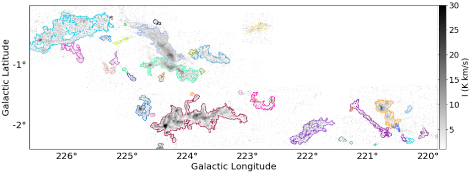
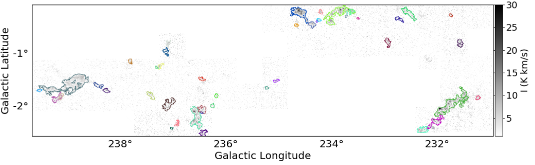
Figure 1: Edge of the MCs of the ¹³CO catalogue  drawn over the integrated intensity map of ¹³CO (1–0)  (intensity bar on the right).

3 Molecular cloud catalogue from ¹³CO (1–0)  data

We used the ¹³CO (1–0)  data cubes to produce a catalogue of MCs, in analogy to the ¹²CO (1–0)  line MCs catalogue presented in Paper I . In our FQS data, the emission of the ¹³CO (1–0) line is less extended than that of the ¹²CO (1–0)  line. As a consequence, we do not detect the low-column density layers of the ¹²CO (1–0)  clouds in the ¹³CO (1–0)  data, and structures that appear connected in ¹²CO (1–0)  can instead be composed of smaller separate clouds in the ¹³CO (1–0)  catalogue. On the other hand, the ¹³CO (1–0)  line has a lower optical depth, typically $<$1 in our data (see Sect. 4). It therefore is a better tracer of the total CO column density than the optically thick ¹²CO. Moreover, several MC catalogues in the literature were derived from ¹³CO (1–0)  data, and this new catalogue will allow us to compare our results with a more homogeneous data-set.

To identify the clouds, as in Paper I , we used the algorithm called Spectral Clustering for Interstellar Molecular Emission Segmentation (SCIMES) (Colombo et al., 2015), which is based on a cluster analysis of dendrograms of 3D (l,b,$\varv$) data cubes. We applied SCIMES to the ¹³CO (1–0)  spectral data cubes from the FB250 filter bank. In order to select well-defined structures and reduce contamination from noisy regions, we masked the cubes by selecting only pixels in which the signal is higher than 5$\times$rms in two consecutive velocity channels. We further extended the mask to include all adjacent pixels in which the signal is higher than 2$\times$rms. We then produced the dendrogram tree of the masked cube. We set the minimum signal in the pixel (min_value) to 0.61 K (equivalent to 3$\times$rms), the minimum difference between two peaks for being considered separate leaves (min_delta) to 8$\times$rms, and the minimum number of pixels of the spectral cube needed for a leaf to be independent (min_npix) to those contained in three times the telescope-beam solid angle. With respect to the set of the SCIMES parameters used in Paper I , we increased the min_value from 2$\times$rms to 3$\times$rms to select only pixels with a well-defined line emission that guarantees a good line fitting and min_delta from 7$\times$rms to 8$\times$rms to reduce the level of fragmentation of the detected structures. We finally applied the spectral clustering using the volume of the isosurface in the (l,b,$\varv$) space as a criterion. Because we were also interested in clouds that may simply have little substructure within them, we also included the single leaves of the dendrogram that had been excluded by the clustering algorithm.

In total, we identified 87 MCs in our ¹³CO (1–0)  FB250 data cubes. Sixty-seven MCs are composed of a single leaf, indicating that they are coherent structures. A view of the position and contours of the identified structures is shown in Fig. 1. For each cloud, we measured the following properties, using the definition in Rosolowsky & Leroy (2006): centroid position in Galactic coordinates; semi-major ($\sigma_{\rm maj}$) and semi-minor ($\sigma_{\rm min}$) axes, estimated as the rms of the intensity-weighted second moments along the direction of maximum cloud extent and its perpendicular direction, respectively; position angle; intensity-weighted velocity; and relative velocity dispersion ($\sigma_{v}$). From the geometrical mean of the semi-axes, we derived the radius of the equivalent spherical cloud as $R=1.91\sqrt{\sigma_{\rm maj}\sigma_{\rm min}}$ (Rosolowsky & Leroy, 2006).

From the central velocity of the ¹³CO (1–0)  line, we derived the kinematic distance of the emitting cloud by applying a Galaxy rotation model. We used the IDL routine of the CPROPS package (Rosolowsky & Leroy, 2006) for the distance estimate, assuming a flat Galactic rotation curve, which is a good approximation for the outer Galaxy, with the solar galactocentric radius $R_{0}$ = 8.34 kpc and rotation velocity $\Theta_{0}$ = 240 km s^-1  (Reid et al., 2014). Because we observe in directions pointing outside of the solar circle, our distance estimate is not affected by the near and far distance ambiguity. We also converted the heliocentric distance into galactocentric radius $R_{\rm gal}$. The mass of the clouds was estimated with three different methods that are described in Sect. 4. To be consistent with Paper I , we used the mass derived from the Herschel  H₂ column density map (Sect. 4.3) to calculate the average mass surface density ($\Sigma$) of the clouds and the virial parameter, $\alpha_{\rm vir}=\frac{5\sigma_{\rm v}^{2}R}{MG}$ (McKee & Zweibel, 1992), where $G$ is the gravitational constant. We derived the velocity dispersion of the gas from the measured full width at half maximum (FWHM) of the ¹³CO (1–0)  line through the relation $\sigma_{\rm v}=FWHM/\sqrt{8\ln(2)}$. We highlight that this is a good estimate of the velocity dispersion because the lines are spectrally resolved, allowing a good measure of the FWHM, and its optical depth is low, with values at the line peak below 3 in 98% of the spatial pixels of the MCS. Moreover, we observe in the direction of a portion of the outer Galaxy in which the cloud crowding is not an issue. In this region the ¹³CO (1–0)  observed lines as well as ¹²CO (1–0)  (Paper I, ) are well fitted with a single-Gaussian profile, and our measurement of the gas velocity dispersion of the single MCs is not affected by blending of emission of possible multiple clouds along the same line of sight.

All the derived parameters are reported in Table 3 for a sub-sample of MCs. The complete table is available in electronic form at the CDS . In the catalogue, we also give the number of leaves identified by the dendrogram that compose the cloud. Because the ¹³CO (1–0)  map is larger than the Herschel  H₂ column density map, which does not cover Galactic latitudes below $\sim$-2°, some clouds identified in the ¹³CO (1–0)  map are only partially covered or not covered at all by the Herschel  H₂ column density map. The mass and surface density derived for these clouds are lower limits and the virial parameter is an upper limit; these clouds are flagged with flag1 = 1 in Table 3. Other clouds extend up to the edge of the ¹³CO (1–0)  map and might therefore not be completely mapped by our observations. For these clouds, identified with flag2 = 2 in Table 3, the measured parameters have an uncertainty that depends on how much CO emission was missed.

4 Mass estimate of molecular clouds

The mass of MCs is derived by integrating the H₂ column density over the projected area in the sky with the relation

$$M=\mu_{\rm H_{2}}m_{\rm H}\int{N{\rm(H_{2})}{\rm d}A},$$ (1)

where $\mu_{\rm H_{2}}$ = 2.8 is the mean molecular weight for a hydrogen molecule that takes into account the presence of helium, $m_{\rm H}$ is the mass of the hydrogen atom, $A$ is the area of the cloud, and $N{\rm(H_{2})}$ is the molecular hydrogen column density. For the clouds of the FQS catalogue, we have different possibilities to derive $N{\rm(H_{2})}$ and, consequently, the mass, either by using the cold dust as a tracer, exploiting the Herschel  data, as we did in Paper I for the MC catalogue derived from ¹²CO (1–0)  emission, or by using the molecular gas as a tracer, exploiting the FQS data. In the following subsections, we describe three different methods that we used to estimate the mass of the clouds, and we compare the results.

4.1 Mass from the ¹³CO column density

The FQS data-set offers the possibility of deriving the mass of the clouds from the ¹³CO (1–0)  line emitted from the molecular gas by deriving the ¹³CO column density and converting it into H₂ column density using the ¹³CO chemical abundance with respect to H₂. We call this mass $M_{N(^{13}\rm CO)}$. We used the mask of the ¹³CO (1–0)  FB250 spectral cube produced by the SCIMES algorithm for the identification of the MCs to define the spatial and spectral range pertinent to each MC, and we derived the H₂ column density map for each MC of the catalogue. We assumed that the emission fills the beam, which is good for the extended emission of gas in MCs, and a uniform excitation temperature within the beam, equal for both ¹²CO (1–0)  and ¹³CO (1–0). This latest assumption is formally correct in local thermal equilibrium (LTE) conditions, although density gradients and non-LTE conditions in local portion of the clouds can lead to differences in excitation temperature of ¹²CO (1–0)  and ¹³CO (1–0). The excitation temperature $T_{\rm ex}$ was derived from the ¹²CO (1–0)  brightness temperature in each (l,b,$\varv$) pixel under the assumption that the ¹²CO (1–0)  emission is optically thick, which is usually the case for MCs, with the formula

$$T_{\rm ex}=\frac{5.53}{{\rm ln}[1+5.53/(T(^{12}{\rm CO})+0.837)]}\leavevmode\nobreak\ [K],$$ (2)

where $T(^{12}{\rm CO})$ is the main-beam brightness temperature of ¹²CO (1–0)  at the (l,b,$\varv$) pixel. This equation includes the subtraction of the cosmic microwave background at $T=$ 2.73 K. The excitation temperature at the peak of the line in the mapped region ranges between 3.6 K and 30.8 K, with a median value of 9.5 K.

The optical depth of the ¹³CO (1–0)  was calculated in each (l,b,$\varv$) pixel from the formula

$$\tau_{13}=-{\rm ln}\left[1-\frac{T(^{13}{\rm CO})]/5.3}{(e^{5.3/T_{\rm ex}}-1)^{-1}-0.16}\right],$$ (3)

where $T(^{13}{\rm CO})$ is the main-beam brightness temperature of ¹³CO (1–0)  in the pixel. We found that the median value of $\tau_{13}$ for all the pixels is 0.2 (0.6 at the peak of the line), with the 5th percentiles of 0.03 and the 95th percentiles of 0.9, indicating that in this portion of the Galactic plane, at the spatial scales probed by our observations (larger than about 0.27 pc for distances larger than 1 kpc), the ¹³CO (1–0)  line is almost always optically thin or moderately thick. It is therefore able to trace the largest part of the molecular gas in the clouds, from which a meaningful estimate of the cloud mass can be derived.

We derived the ¹³CO (1–0)  column densities at each (l,b) pixel with the following formula:

$$N(^{13}{\rm CO}){\rm[cm^{-2}]}=2.6\times 10^{14}\int{\frac{\tau_{13}T_{\rm ex}}{1-e^{\frac{-5.3}{T_{\rm ex}}}}{\rm d}\varv\leavevmode\nobreak\ [\rm K\leavevmode\nobreak\ km\leavevmode\nobreak\ s^{-1}]}.$$ (4)

The ¹³CO (1–0)  column density map was then converted into H₂ column density map by assuming a relative chemical abundance of [¹³CO]/[H₂] = 1.4$\times$10^-6 (Frerking et al., 1982). The mass of the MCs was calculated with Eq. 1.

4.2 Mass from the integrated ¹²CO (1–0)  line emission

A method that is commonly used in the literature to derive the H₂ column density when only the ¹²CO (1–0)  line is available is to use the empirical relation between $N$(H₂) and the integrated intensity of the ¹²CO (1–0)  line, $I(^{12}{\rm CO})$, that is,

$$N({\rm H_{2}})=X(^{12}{\rm CO})\,I(^{12}{\rm CO}),$$ (5)

where $X(^{12}{\rm CO})$ is the CO-to-H₂ conversion factor. Many studies have been conducted to derive this factor with different methods. In this paper, we assumed the widely used value $X(^{12}{\rm CO})=2\times 10^{20}$ cm^-2 (K km s^-1)^-1, which has been recommended by Bolatto et al. (2013) in his review paper. We call the mass derived with this method $M_{X(^{12}{\rm CO})}$. In order to correctly compare this mass with the one derived in the previous section, we integrated the ¹²CO (1–0)  line emission in the same area of the cloud, that is, the one defined by the ¹³CO (1–0)  emission. Recent papers have shown that when measured in new-generation CO surveys, with arcminute or sub-arcminute spatial resolution, the CO-to-H₂ conversion factor spans more than one order of magnitude from pixel to pixel (e.g. Barnes et al. 2015; Schuller et al. 2017; Paper I ) due to local differentiation of the physical conditions between the clouds and within the same MC when it is spatially well resolved. However, in general, the mean value agrees within the error with the standard value.

4.3 Mass from the FIR dust emission

The third option to derive the mass of the MCs of the FQS catalogue, which we applied in Paper I , is to use the H₂ column density derived from the Herschel  photometric data. We refer to this mass as $M_{\rm dust}$. The Herschel  H₂ column density maps were derived from the fitting of the spectral energy distribution (SED) of the cold dust in the wavelength range from 160 $\mu$m  to 500 $\mu$m  (Schisano et al., 2020), under the assumption of a gas-to-dust ratio of 100 and a dust opacity law of $\kappa_{\lambda}=\kappa_{\rm 300}\leavevmode\nobreak\ (\lambda/300\leavevmode\nobreak\ \mu m)^{-\beta}$ with $\kappa_{\rm 300}$=0.1 cm²g^-1 and a grain emissivity parameter $\beta$=2 (Hildebrand, 1983). The Herschel  maps have a spatial resolution of 36″, which is similar to that of the FQS data, and they were convolved and regridded to match the FQS products. Being derived from photometric data, Herschel  H₂ column density map cannot disentangle clouds at different distances that overlap along the same line of sight. In our FQS ¹³CO catalogue, only eight MCs have a small spatial overlap with another cloud, as shown in Fig. 1. In the overlapping spatial pixels, we distributed the total H₂ column density of the Herschel  map among the two cospatial clouds in proportion to their ¹³CO (1–0)  intensity. This is a reasonable approach because the ¹³CO (1–0)  emission is optically thin in our data-set, as shown in Sect. 4.1, and in this case, the emission is proportional to the column density.

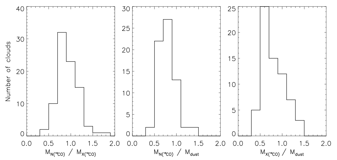
Figure 2: Histograms of the ratios of the cloud mass estimates with three different methods. Left: Ratio of the mass derived from the $N(^{13}\rm CO)$ column density and that from $X(^{12}{\rm CO})$. Centre: Ratio of the mass derived from the $N(^{13}\rm CO)$ and that from the Herschel-based H₂ column density, which traces the cold dust. Right: Ratio of the mass derived from $X(^{12}{\rm CO})$ and that from the Herschel-based H₂ column density.

Table 1: Ratio of the masses of the MCs of the ¹²CO catalogue  derived with different methods.

mass ratio	median	10th percentile	90th percentile
$M_{N(^{13}\rm CO)}$ / $M_{X(^{12}{\rm CO})}$	0.99	0.76	1.36
$M_{N(^{13}\rm CO)}$ / $M_{\rm dust}$	0.86	0.66	1.15
$M_{X(^{12}{\rm CO})}$ / $M_{\rm dust}$	0.86	0.61	1.34

4.4 Comparison of the three mass estimates

The masses of the MCs of the FQS catalog derived with the three methods are reported in Table 3. We point out that the three masses are calculated in the same projected area onto the plane of the sky for each cloud. In Fig. 2, we show the distribution of their ratios, $M_{N(^{13}\rm CO)}$ / $M_{X(^{12}{\rm CO})}$, $M_{N(^{13}\rm CO)}$ / $M_{\rm dust}$ , and $M_{X(^{12}{\rm CO})}$ / $M_{\rm dust}$, and in Table 1, we report the median values and the 10th and 90th percentiles of these ratios. In general, we find a good agreement between the mass estimates, with ratios ranging from 0.4 to 1.9. In particular, the masses derived from CO data with $N(^{13}\rm CO)$ and $X(^{12}{\rm CO})$ are very similar, with a narrow distribution of their ratio centred at the median value of 0.99. This indicates that at the sensitivity level of our survey, the two lines ¹²CO (1–0)  and ¹³CO (1–0) in general trace a similar column of gas. ¹³CO (1–0)  loses only the more tenuous outskirts of the clouds, which contribute little to the total cloud mass. Moreover, the similarity of these two mass estimates indicates that despite the high variability of the CO-to-H₂ conversion factor at the pixel level (Paper I, ), the assumption of a constant value for $X(^{12}{\rm CO})$ is a valid method for deriving the total mass in extended structures as the MCs, at least in this portion of the Milky Way. On the other hand, for the majority of the MCs, the mass derived from the CO gas is lower than that derived from the cold dust, with a median value of 0.86 for both $M_{N(^{13}\rm CO)}/M_{\rm dust}$ and $M_{X(^{12}{\rm CO})}/M_{\rm dust}$. The same trend was also found by other authors who analysed CO data collected with different telescopes (NANTEN, Elia et al. 2013 and MOPRA, Olmi et al. 2016) in some of the regions of the Galactic plane that are mapped in FQS. This is likely because the cold dust at the far-infrared wavelengths of the Herschel  observations is a truly optically thin tracer that is more effective in tracing all the material along the line of sight than CO because ¹²CO (1–0)  is usually optically thick in MCs and also ¹³CO (1–0), in spite of its lower opacity, becomes optically thick in the densest regions such as clumps and cores.

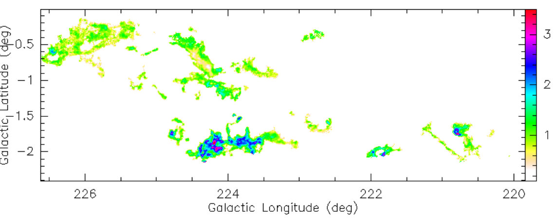
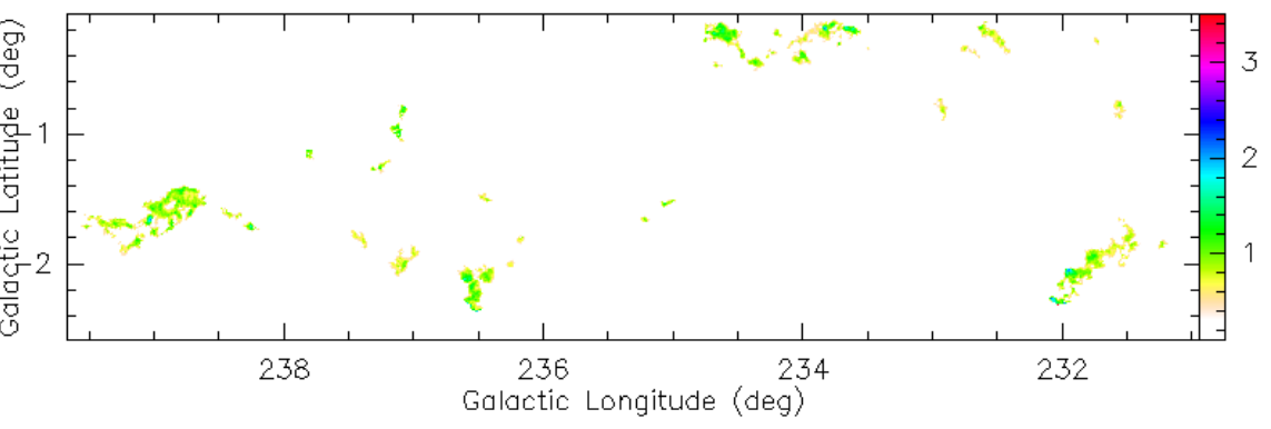
Figure 3: $N{(\rm H_{2}})_{N(^{13}\rm CO)}/N{(\rm H_{2}})_{\rm dust}$ ratio (right colour bar) in the $l$ = 220°–226$\aas@@fstack{\circ}$6 field (top) and that in the $l$ = 231°–239$\aas@@fstack{\circ}$7 field (bottom).

When comparing mass estimates, we need to take the sources of uncertainty into account that come from the assumptions that we made in deriving masses. On the one hand, for the CO-based mass estimates, we assumed a constant CO abundance for all the clouds, while region-to-region variations can occur depending on the chemical evolutionary stage and on the local physical conditions. We also assumed the same excitation temperature for ¹²CO (1–0)  and ¹³CO (1–0), while density gradients and non-LTE conditions can lead to differences in the excitation temperature of the two lines. On the other hand, for the dust-based mass estimates, we assumed a homogeneous dust opacity law, but differences within regions can exist due to the different properties of the dust grains and their state of growth. Moreover, there is evidence that the dust opacity depends on the H₂ column density (e.g. Martin et al. 2012; Roy et al. 2013) and that the grain emissivity parameter $\beta$, which gives the dependence of the opacity on the frequency, is anti-correlated with the temperature (e.g. Dupac et al. 2003; Désert et al. 2008; Juvela et al. 2015). Schisano et al. (2020) have shown that assuming a value of $\beta$ = 1.8 (which should be more appropriate for regions with higher temperature between $\sim$ 15 – 20 K) instead of $\beta$ = 2 (which should be more appropriate for colder regions with temperature between $\sim$ 10 –15 K) has the effect of decreasing the column density by about 20% and increasing the temperature by about 6%. Additionally, Pezzuto et al. (2021) have shown that when the temperature of the dust is higher than 20 K, the SED fitting of the four Herschel bands with $\lambda\geq$ 160 $\mu$munderestimates the true dust temperature, and as a consequence, overestimates the H₂ column density. Finally, there are some indications that the gas-to-dust ratio decreases with galactocentric radius (Giannetti et al., 2017). However, in our set of data, we do not find any correlation of the $M_{N(^{13}\rm CO)}$ / $M_{\rm dust}$ ratio with the galactocentric radius. This suggests that either there is no significant variation of the CO chemical abundance and the gas-to-dust ratio with distance in the first $\sim$ 6 kpc of the surveyed slice of the outer Galaxy or, less likely, that both the CO chemical abundance and the gas-to-dust ratio change with distance with the same trend. However, we must point out that the statistics at the larger distance is poor because our sample only includes six MCs with $R_{\rm gal}>$ 11.3 kpc (see the last panel of Fig. 4). We do not find any correlation either of the ratio of the mass derived from CO and from dust with the integrated intensity of ¹²CO (1–0)  and with the dust temperature.

In order to further explore the possible presence of the effects listed above in specific regions, we compared pixel-by-pixel the $N{(\rm H_{2}})$ maps derived from ¹³CO (1–0)  FQS data ($N{(\rm H_{2}})_{N(^{13}\rm CO)}$) with those derived from the SED fitting of the Herschel  data ($N{(\rm H_{2}})_{\rm dust}$). The $N{(\rm H_{2}})_{N(^{13}\rm CO)}$ map was built by stacking all the maps of the 87 MCs of the catalogue. In Fig. 3 we show the pixel-by-pixel $N{(\rm H_{2}})_{N(^{13}\rm CO)}/N{(\rm H_{2}})_{\rm dust}$ ratio. We find that 65$\%$ of the pixels have $N{(\rm H_{2}})_{N(^{13}\rm CO)}/N{(\rm H_{2}})_{\rm dust}<$ 1, while only a small portion of the mapped area (4$\%$ of pixels) has $N{(\rm H_{2}})_{N(^{13}\rm CO)}/N{(\rm H_{2}})_{\rm dust}>$2. We note that the pixels with this high ratio belong to only four MCs: FQS-MC220.716-1.783 (index = 8) at ($l\simeq$220.7°, $b\sim$-1.8°), FQS-MC221.959-2.092 (index = 14) at ($l\simeq$221.9°, $b\sim$-2.1°), FQS-MC223.966-1.904 (index = 24) at ($l\simeq$224° $b\sim$-1.9°), and FQS-MC224.750-1.769 (index = 32) at ($l\simeq$224.8°, $b\sim$-1.8°). These are the regions with the brightest CO emission (Figs. 6 and 8 in Paper I ) and the highest CO excitation temperature ($T_{\rm ex}\geq$ 12 K) as well as high dust temperature, suggesting that the presence of warm gas could affect the observed ratio. In MCs with index 8, 14, and 32, only a small portion of their projected area has $N{(\rm H_{2}})_{N(^{13}\rm CO)}/N{(\rm H_{2}})_{\rm dust}>$2, while in the cloud FQS-MC223.966-1.904, the H₂ column density derived from CO in most of the area is higher than that derived from the dust. This is the MC with the brightest ¹²CO (1–0)  emission in the surveyed area, and it also appears bright in the Herschel  maps. This MC is part of the CaM OB1 association and roughly corresponds to the Sh 2-296 nebula, which is rich in gas ionised by the close-by O-type stars (Fernandes et al., 2019). Two H II regions are present in this area, S296 and S292 (Sharpless, 1959). For this region, both the $T_{\rm ex}$ estimated from ¹²CO (1–0)  and the dust temperature derived from the SED fitting of the Herschel  fluxes are the highest of the whole surveyed region, with values between $\sim$ 15 K and $\sim$ 29 K, respectively. At this temperature, the mass derived from Herschel  data is likely underestimated, which makes the measured $N{(\rm H_{2}})_{N(^{13}\rm CO)}/N{(\rm H_{2}})_{\rm dust}$ an upper limit. This high temperature and the presence of ionised gas may modifiy the chemical abundance and/or different properties of the dust grains in this particular cloud, which might explain the high measured $N{(\rm H_{2}})_{N(^{13}\rm CO)}/N{(\rm H_{2}})_{\rm dust}$ ratio. A substantial modification of the chemical abundance ratio of ¹³CO and C¹⁸O in the region that corresponds to our MC FQS-MC223.966-1.904 with respect to its adjacent clouds was found by Lin et al. (2021) as well.

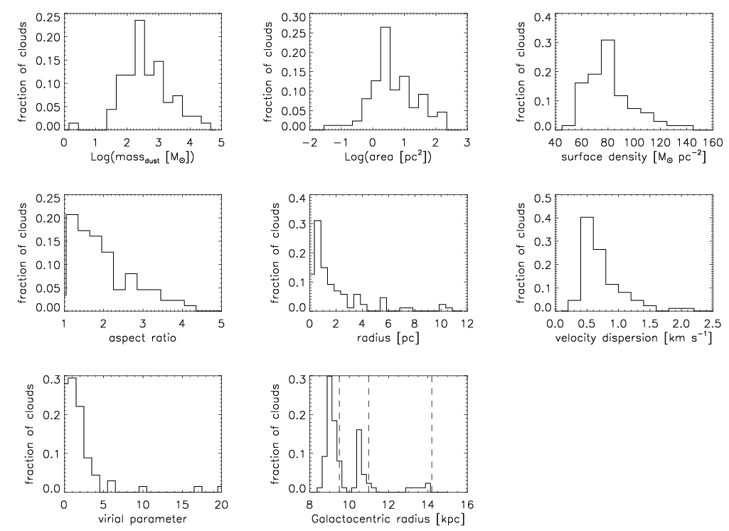
Figure 4: Histograms of the distributions of the derived physical properties for the MCs of the FQS ¹³CO catalogue. Top left: Masses derived from cold dust emission. Top centre: Area. Top right: Average mass surface density. Middle left: Aspect ratio ($\sigma_{\rm maj}$ / $\sigma_{\rm min}$). Middle centre: Equivalent spherical radius. Middle right: Velocity dispersion. Bottom left: Virial parameter. Bottom centre: galactocentric radius. The vertical dashed lines indicate the reference position of the Local Arm (Xu et al., 2013), Perseus Arm (Choi et al., 2014), and Outer Arm (Hou & Han, 2014) at the central Galactic longitude of the surveyed region $l$ = 230°.

Table 2: Statistical physical properties of the MCs of the FQS catalogue derived from the ¹³CO (1–0)  data.

	median	mode
massdust (M⊙)	443	251
area (pc2)	4.7	2.5
surface density (M⊙  pc-2)	86	80
aspect ratio	2.0	1.2
equivalent spherical radius (pc)	1.4	0.6
velocity dispersion (km s-1)	0.7	0.5
virial parameter	1.87	1.00
heliocentric distance (kpc)	1.57	0.89
galactocentric radius (kpc)	9.33	9.00

5 Analysis of the ¹³CO (1–0)  molecular cloud catalogue

5.1 Global properties

In Fig. 4 we show the histograms of some of the physical parameters of the MCs, and in Table 2 we list the median and modal values of these parameters. The MCs are distributed along a heliocentric distance from 0.39 kpc to 7.74 kpc, which corresponds to a galactocentric radius from 8.64 kpc to 14.15 kpc. The clouds are gathered into three groups that correspond to the three spiral arms of the Milky Way (Local, Perseus, and Outer arms), which are well visible in the last panel of Fig. 4. Because of the different distances, the minimum detectable size of the clouds changes significantly in the three arms. In particular, all the MCs of the catalogue have a projected area on the sky that is larger than twice the area of the telescope beam, which corresponds to a minimum area from 0.16 pc² at 1 kpc to 10.31 pc² at 8 kpc.

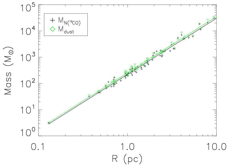
Figure 5: Plot of the the mass of the MCs $\it vs$ their radius. The mass derived from the ¹³CO column density is indicated with black pluses, and the mass derived from Herschel  -based H₂ column density is indicated with green diamonds. The linear fit in the log-log axes for the two data-sets is shown by the straight lines.

In Fig. 5 we show the mass-radius relation for the MCs of the FQS catalogue with masses derived from both the gas (namely FQS data) and dust (Herschel  data). The masses and radii are well correlated, with a power law of the type $M\propto R^{D}$ with the exponent $D$ = 2.13$\pm$0.04 for the masses derived from CO and $D$ = 2.14$\pm$0.03 for the masses derived from dust. The two exponents (derived with the robust_linefit IDL procedure) are consistent within the statistical error and similar to that previously derived in the catalogue of MCs of GRS $D$ = 2.36$\pm$0.04 (Roman-Duval et al., 2010). The strict correlation between mass and radius with a power-law exponent close to 2 leads to a range in mass surface density where the minimum and maximum values differ by only a factor of $\sim$ 2 with respect to the modal value of 80 M_⊙  pc^-2. From this correlation, we can find the minimum detectable mass that corresponds to the minimum detectable area at the various distances, that is, 10 M_⊙  at 1 kpc and 880 M_⊙  at 8 kpc. The minimum area and mass at the largest distance ($\sim$ 8 kpc) roughly correspond to the values below which the respective distributions invert the slope (see Fig. 4), which indicates that our sample is incomplete below these values.

We note that about 60% of our MCs have a virial parameter smaller than two, which is the critical value below which a structure is gravitationally bound. This indicates that in the majority of the identified clouds, gravity plays a major role in their confinement.

5.2 Comparison between the FQS molecular cloud catalogues from ¹²CO (1–0) and ¹³CO (1–0)

In this subsection, we compare the properties of the MCs catalogue derived from the ¹³CO (1–0)  data with those derived from the ¹²CO (1–0)  line in the same region (Paper I, ). Because the two lines have a slightly different critical density and optical depth, they trace gas with different physical properties and therefore different parts of the same structure. It is therefore interesting to compare the two FQS catalogues to understand how the measured physical parameters of the MCs change in the two catalogues and to determine whether they can lead to different conclusions about the status of the cloud itself, for example, whether they are gravitationally bound structures.

In our FQS data, the area in which ¹³CO (1–0)  emission is detected is smaller than that in which ¹²CO (1–0)  emission is detected because the ¹³CO chemical abundance is lower (see Figs. from 6 to 9 in Paper I ). On the other hand, the lower opacity of ¹³CO (1–0)  allows us to probe a deeper column of gas inside the cloud, with a higher particle density than for the ¹²CO (1–0)  line. As a consequence, the structures traced by the ¹³CO (1–0)  line are the brightest and densest parts of the ¹²CO (1–0)  structures, while low-brightness regions in ¹²CO (1–0)  are mostly undetected in ¹³CO (1–0). Moreover, extended ¹²CO (1–0)  MCs with an internal substructure may become decomposed in separate clouds in the ¹³CO catalogue. We find that 35 out of the 267 MCs of the ¹²CO catalogue  (i.e. 13%) have one or more counterparts in the ¹³CO catalogue. For these MCs, we show in Fig. 6 the distribution of how many ¹³CO MCs are associated with any single ¹²CO MC. In general, there is a one-to-one association, but 13 ¹²CO MCs are composed of two or more ¹³CO MCs. This last group is composed of ¹²CO MCs that show substructures, being formed by more than one leaf that are clustered together by the SCIMES algorithm. It is worth noting that in our FQS data, for each ¹²CO MC with at least one associated ¹³CO MC, the percentage of the (l,b,$\varv$) cube that has a ¹²CO (1–0)  signal above 2$\times$ rms(¹²CO (1–0)) and also contains ¹³CO (1–0)  signal above 3$\times$ rms(¹³CO (1–0)) is low, between 1% and 47% (bottom panel of Fig. 6). This confirms that only the brightest ¹²CO (1–0)  emission is also detected in ¹³CO (1–0).

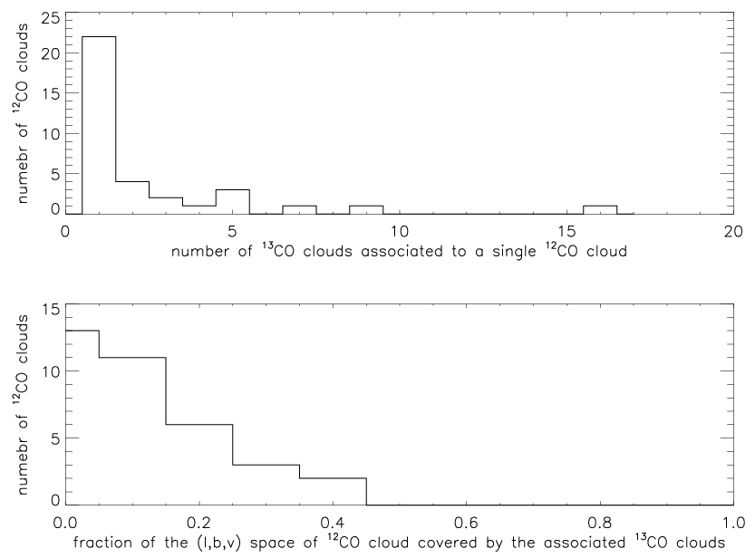
Figure 6: Top: Histogram of the number of ¹³CO MCs associated with a single ¹²CO MC. Bottom: Histogram of the fraction of the (l,b,$\varv$) space of ¹²CO MC covered by the associated ¹³CO MCs.

Comparing the median and modal values of the main physical parameters in the two FQS catalogues, we find that in general, the ¹³CO (1–0)  clouds (Table 2) are smaller and less massive than those identified in the ¹²CO (1–0)  catalogue (Table 1 in Paper I ), while the surface density of the structures traced by ¹³CO (1–0)  is slightly higher than that of the ¹²CO (1–0), as expected. On the other hand, the median and modal values of the aspect ratio ($\sigma_{\rm maj}$ / $\sigma_{\rm min}$), equivalent spherical radius, velocity dispersion and virial parameter are similar in the two catalogues, as well as their parameter range and the shape of the distributions. In particular, it is interesting to compare the values of the velocity dispersion derived from the FWHM of ¹²CO (1–0)  and ¹³CO (1–0)  since the first line has a higher optical depth than the second and it is well known that velocity dispersion of the gas derived from the FWHM of an optically thick line tends to be overestimated by a factor that increases with the line opacity (Hacar et al., 2016).

In Fig. 7 we show the ratio of the velocity dispersion derived from the FWHM of the ¹²CO (1–0)  and ¹³CO (1–0)  lines in each pixel. As expected, for most of the pixels, the velocity dispersion derived from the line with higher opacity, ¹²CO (1–0), is larger. However, the difference is small, with a median ratio of 1.4. This indicates that the velocity dispersion of the MCs of the ¹²CO catalogue  of Paper I is a stringent upper limit of the real velocity dispersion of the gas. In Paper I we discussed the relation between the velocity dispersion and the radius of the MCs, known as the first Larson relation (Larson, 1991), which is expected to be of the form $\sigma_{v}\propto R^{\beta}$ with $\beta$ = 0.5, if the origin of the gas motions is purely supersonic turbulence, the so-called Burgers turbulence (McKee & Ostricker, 2007). For the MCs of the ¹²CO catalogue,  we found two regimes: for $R\geq$ 2 pc, the velocity dispersion increases with radius with an exponent $\beta$ = 0.59, similar to what is expected from pure supersonic turbulence, while for $R<$ 2 pc, the relation is almost flat, with $\beta$ = 0.08, similar to what is found in massive clumps (Traficante et al., 20018a, 2018b), suggesting that gravity already plays an important role at these scales, as also suggested by the values of the virial parameter we estimated. This behaviour was also observed in the MC catalogue derived for the Milky Wave plane in the Galactic longitude range 104$\aas@@fstack{\circ}$75 $<l<$ 119$\aas@@fstack{\circ}$75 (Ma et al., 2021).

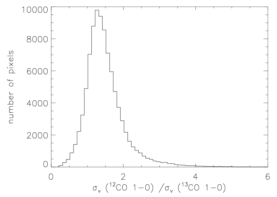
Figure 7: Histogram of the ratio of the velocity dispersion derived from the FWHM of the ¹²CO (1–0)  and ¹³CO (1–0)  lines.

We repeated this analysis for the MCs detected in this paper, which represent the densest part of some of the largest clouds of Paper I . The result is shown in Fig. 8. The limited number of MCs and the restricted radius range prevent the detection of a clear trend. The observed distribution seems to be compatible with the behaviour found for the ¹²CO catalogue  clouds (shown as dotted and dashed lines in Fig. 8) and also with an only supersonic turbulent regime, indicated by the solid line that is the best fit of the relation $\sigma_{v}=aR^{\beta}$ in the full radius range, whose coefficients are: $a$ = 0.67 and $\beta$ = 0.4. The Pearson coefficient is also similar in both cases, 0.4 in the case of two power laws and 0.6 in the case of a single power law. This show a low degree of correlation between the two parameters for the clouds of the ¹³CO catalogue.

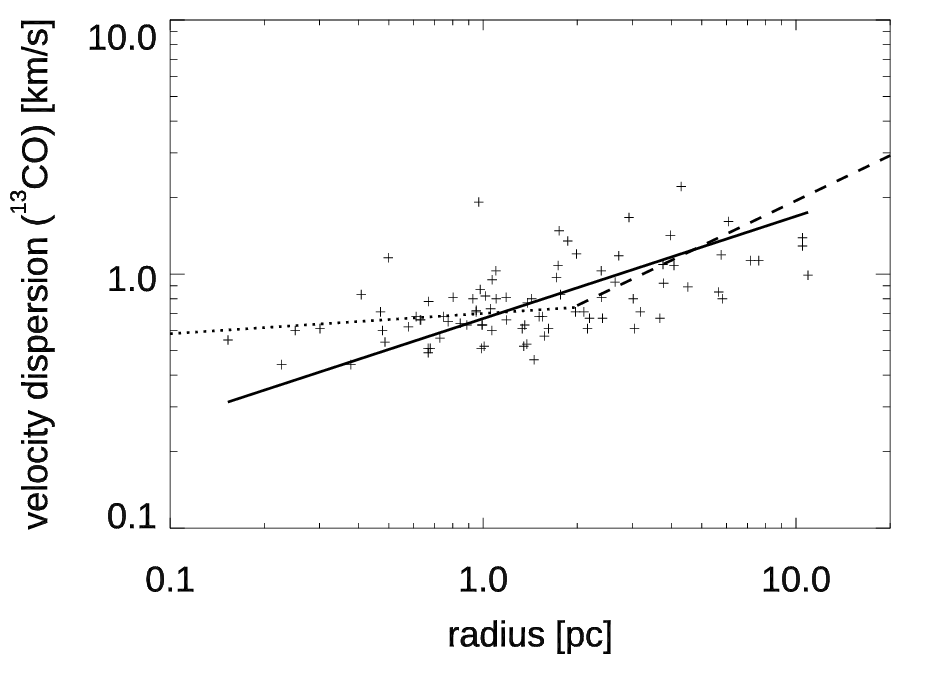
Figure 8: Radius vs velocity dispersion plot of MCs of the ¹³CO catalogue. The solid line represents the best fit for the relation $\sigma_{v}=aR^{\beta}$ in the full radius range. The best-fit coefficients are $a$ = 0.67 and $\beta$ = 0.4. The dotted and dashed lines correspond to the relations derived in Paper I for the ¹²CO catalogue  rescaled to this set of data: $a$ = 0.7 and $\beta$ = 0.08 for $R<$ 2 (dotted line), and $a$ = 0.5 and $\beta=$ 0.59 for $R>$ 2 (dashed line).

Another interesting comparison regards the virial parameter derived from the two catalogues, which is used to evaluate the role of gravity in the confinement of the clouds. In Fig. 9 we show the plot of the virial parameter of the ¹²CO (1–0)  MCs that have at least one ¹³CO (1–0)  associated MC, against the virial parameter of all the associated ¹³CO (1–0)  MCs. The virial parameters of the ¹³CO (1–0)  clouds associated with the same single ¹²CO (1–0)  cloud are connected by a dotted vertical line in Fig. 9. When we exclude the ¹²CO (1–0)  clouds with many ¹³CO (1–0)  sub-structures, the two virial parameters are well correlated. The virial parameter derived from ¹³CO (1–0)  is similar to or slightly lower than that derived from ¹²CO (1–0). This confirms that the fraction of the cloud traced by ¹³CO (1–0)  is the densest and hence more gravitationally bound part. We calculated the ratio of the virial parameters derived from the ¹²CO (1–0)  with respect to that derived from ¹³CO (1–0)for the ¹²CO MCs associated with only one ¹³CO cloud. We found a mean value $<\alpha_{\rm vir}[^{12}\rm CO(1-0)]/\alpha_{\rm vir}[^{13}\rm CO(1-0)]>$ = 1.3, that is, a value similar to the mean ratio of the velocity dispersion discussed above. This modest difference likely arises because in the surveyed portion of the Galactic plane, the H₂ column density is not particularly high ($\leq$ 5$\times 10^{22}$ cm^-2), leading to a CO emission that does not have a very high optical depth. Moreover, the effects of the different line opacity between the two tracers are small. Our conclusions cannot be generalised to the entire Milky Way, however, because zones of the Galactic plane with higher H₂ column density and particle density may have more different velocity dispersions and virial parameters.

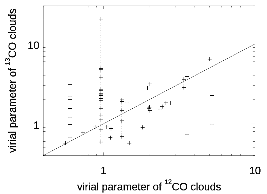
Figure 9: Plot of the virial parameter of the ¹²CO (1–0)  MCs that have at least one ¹³CO (1–0)  associated MC, with the virial parameter of the associated ¹³CO (1–0)  MC(s). Only the sub-sample of MCs with a valid determination of the virial parameter (flag1=0 in Table 3) are plotted. Dotted vertical lines connect the virial parameters of the ¹³CO MCs associated with the same single ¹²CO MC. The solid straight line indicates the equivalence of the two parameters.

6 Surface density versus galactocentric radius

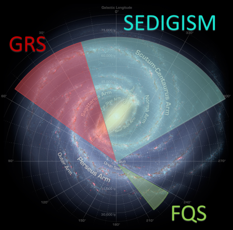
Figure 10: Artistic representation of the Milky Way. The Galactic longitude range covered by three spectroscopic surveys is indicated with coloured slices: red for GRS (Jackson et al., 2006), cyan for SEDIGISM (Schuller et al., 2017), and green for FQS (Paper I, ).

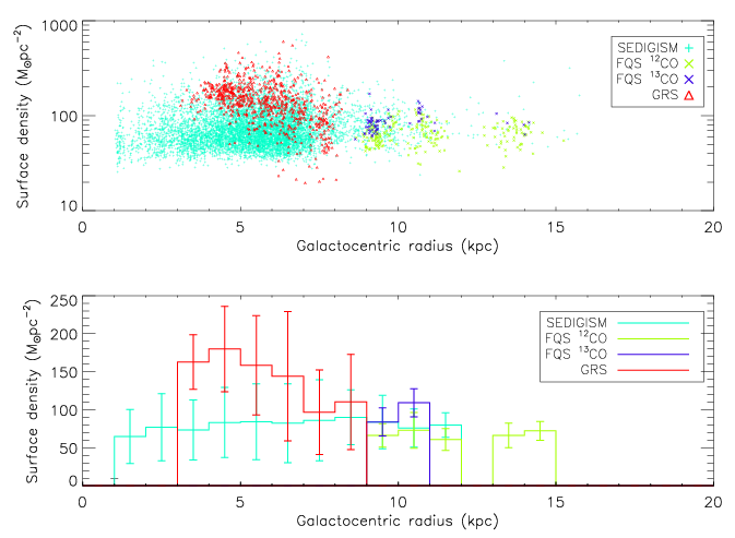
Figure 11: Top: Plot of the mass surface density vs galactocentric radius for the MCs of the SEDIGISM catalogue (cyan plus, Duarte-Cabral et al. 2021), FQS ¹²CO catalogue  (green crosses, Paper I ), FQS ¹³CO catalogue  (blue crosses, this paper), and GRS (red triangles, Roman-Duval et al. 2010. Bottom: Histograms of the mean value of the data shown in the top panel in 1 kpc bins, for bins with more than ten sources. The error bars are the statistical standard deviations in each bin.

One of the essential but not sufficient conditions for activating star formation inside an MC is that enough mass must be gathered in some part of the cloud. An easy observable of this property is the mass surface density. The variation in mass surface density of the MCs with galactocentric radius has been studied by several authors (Miville-Deschênes et al., 2017; Roman-Duval et al., 2010), who have found a decline in molecular cloud mass surface density at $R_{\rm gal}\gtrsim$ 6 kpc. Interestingly, a decrease in mass surface density from the inner to the outer Galaxy was also observed for protostars and pre-stellar cores/clumps (Elia et al., 2021), indicating a lower star formation activity in the outer portion of the Milky Way. We used our FQS MC catalogues together with catalogues produced from homogeneous data of new-generation spectral surveys to study the variation in surface density of the MCs across the Galaxy in a large galactocentric radius range. In particular, we used the Roman-Duval et al. (2010) catalogue, extracted from the GRS data (line ¹³CO (1–0), Galactic longitude range 18°$<l<$ 55$\aas@@fstack{\circ}$7, angular resolution 46″, velocity resolution 0.21 km s^-1, $R_{\rm gal}$ = 3 – 8 kpc, and extractor algorithm CLUMPFIND) and the Duarte-Cabral et al. (2021) catalogue based on the SEDIGISM data (line ¹³CO (2–1), Galactic longitude range -60°$<l<$ 18°, angular resolution 30″, velocity resolution 0.25 km s^-1, $R_{\rm gal}$ = 1 – 15 kpc, and extractor algorithm SCIMES). In Fig. 10 we show the Galactic longitude range covered by the three considered surveys: FQS, GRS, and SEDIGISM, which corresponds to $\sim$ 40% of the total range.

The mean value of the mass surface density of the MCs of the three catalogues is 87$\pm$55 M_⊙  pc^-2, which can be considered as the reference value for the Milky Way. We note that the mean value derived from FQS data perfectly agrees with the total mean value. In Fig. 11 we show the relation of the mass surface density of MCs with $R_{\rm gal}$, together with the histograms of the surface density mean value in 1 kpc bins. In order to have a minimum statistical value, we considered only bins with more than ten sources. For the MCs of the FQS ¹²CO catalogue  (green symbols) and ¹³CO catalogue  (blue symbols), we find that the mean value of the mass surface density is constant in the range $\sim$ 8 – 16 kpc, with a slightly higher value for the MCs of the ¹³CO catalogue  compared to those of the ¹²CO catalogue. Our FQS data agree with the flat trend of the mean mass surface density of the SEDIGISM catalogue (cyan symbols), covering both the inner and outer Galaxy, and at $R_{\rm gal}$ = 9 kpc connect well with the trend of the GRS data, which start to decrease at $R_{\rm gal}\gtrsim$ 6 kpc. Conversely, in the inner Galaxy, the GRS mean values are higher than the SEDIGISM mean values, and in the range 3 $\lesssim R_{\rm gal}\lesssim$ 6 kpc, they are not consistent at the $1\sigma$ level. Interestingly, we find a variability range of the MC mass surface density of about one order of magnitude in the whole range of the investigated Galactocentric radii. The highest values of the SEDIGISM clouds are compatible with the values of the GRS clouds (see Fig. 11). This is an indication that this parameter, which is strictly related to the capability of a cloud to form stars, is determined more by local conditions than by the distance of the cloud from the centre of the Galaxy.

It is worth noting that the measured mass surface density of the MCs can be affected by the crowding level of clouds. Indeed, in highly crowded regions, such as the central part of the Galaxy and the tips of the bar, it is more difficult to properly separate structures along the same line of sight. This leads to a possible overestimate of the cloud mass and consequently of the mass surface density. This effect might explain the prevalence in GRS data of a mass surface density higher than $\sim$ 100 M_⊙  pc^-2 (see Fig. 10). The GRS spans the Galactic longitude range 18°$<l<$ 55$\aas@@fstack{\circ}$7, which is largely covered by the tip of the bar, while SEDIGISM covers a much wider range -60°$<l<$ 18°, which includes part of the bar with the other tip, but also lines of sight that do not cross the central region of the Galaxy and therefore are less crowded. FQS includes only the outer Galaxy with a low level of crowding. As demonstrated by Veneziani et al. (2017), the tips of the bar show an enhanced star formation rate with respect to background and foreground regions because of the large amount of dust and molecular material they contain. This can contribute to the higher mean mass survey density of MCs measured in the GRS catalogue.

We must consider that the sensitivity level and the method we used to derive the cloud mass is different for the three catalogues. The GRS survey has a sensitivity of about a factor 2 better than FQS and a factor 5 better than SEDIGISM, although it observes the ¹³CO (2-1) line. To derive mass, SEDIGISM used the same method as described in Sect. 4.2, with the CO-to-H₂ conversion factor $X(^{13}{\rm CO(2-1)})$ = 10²¹ cm^-2 (K km s^-1)^-1, derived from the comparison with the Herschel  H₂ column density maps (Schuller et al., 2017). The mass surface density in our FQS catalogue is calculated from the mass derived from the Herschel  data, as described in Sect. 4.3. This means that both FQS and SEDIGISM used the Herschel  H₂ column density as a mass calibrator. On the other hand, the cloud mass in GRS is derived from the ¹³CO column density multiplied with the ¹³CO chemical abundance of 1.77$\times$10^-6, which is the method described in Sect. 4.1, but with a different abundance. Finally, while the FQS and SEDIGISM catalogues are produced with the same cloud identification algorithm, SCIMES, the GRS catalogue used a different algorithm, CLUMPFIND. A comparison of the performance of the two algorithms in detecting MCs in the same region was made by Colombo et al. (2015), who found that the two algorithms perform differently and that CLUMPFIND tends to overdivide the molecular emission into smaller structures with respect to SCIMES. In conclusion, the FQS and SEDIGISM catalogues are more homogeneous, while a direct comparison with the GRS catalogue requires more caution.

7 Conclusions

We presented a catalogue of MCs extracted from the ¹³CO (1–0) data cubes at a spectral resolution of 1 km s^-1  of the FQS survey, covering the Galactic plane in the range 220°$<l<$240°  and -2$\aas@@fstack{\circ}$5$<b<$0°. The catalogue contains 87 MCs, for which the main physical parameters, such as area, mass, distance, velocity dispersion and virial parameter, were derived. Making use of available ancillary data, that is, the FQS ¹²CO (1–0)  emission and the Herschel  $N({\rm H_{2}})$ column density map, we applied three different methods to derive the MC mass and compared the results. In general, we find a good agreement between the three different mass estimates. In particular, the masses derived from CO data with $N(\rm^{13}CO)$ and $X(\rm^{12}CO)$ are almost similar, with a narrow distribution of their ratio centred at the median value of $<M_{N(^{13}\rm CO)}/M_{X(^{12}{\rm CO})}>$ = 0.99, indicating that the less extended ¹³CO (1–0)  emission loses only the more tenuous outskirts of the clouds, which contribute little to the total cloud mass. On the other hand, for most of the MCs, the mass derived from the CO gas is lower than that derived from the cold dust, with median values of $<M_{N(^{13}\rm CO)}/M_{\rm dust}>$ = 0.86 and $<M_{X(^{12}{\rm CO})}/M_{\rm dust}>$ = 0.86. In limited areas, we find that $M_{N(^{13}\rm CO)}/M_{\rm dust}\geq$ 2, likely due to a modification of the CO chemical abundance and/or dust grain emissivity related to the high temperature and ionisation level of these regions.

We compared the physical parameters of the MCs of the FQS catalogue extracted from ¹³CO (1–0)  with those derived from ¹²CO (1–0)  presented in Paper I and found that the structures traced by the ¹³CO (1–0)  emission are associated with the brightest and densest regions of the ¹²CO (1–0)  structures, while the structures faint in ¹²CO (1–0)  remain undetected in ¹³CO (1–0). In particular, we found that 35 out of the 267 MCs of the ¹²CO catalogue  have at least one counterpart in the ¹³CO catalogue. For these clouds, not more than 50% of the (l,b,$\varv$) cube with ¹²CO (1–0)  emission is also covered by ¹³CO (1–0)  emission. As a consequence, the ¹³CO (1–0)  MCs are smaller and less massive than the ¹²CO (1–0)  MCs, while the mass surface density of the structures traced by ¹³CO (1–0)  is slightly higher than the mass traced in ¹²CO (1–0). On the other hand, the median and modal values of the aspect ratio, equivalent spherical radius, velocity dispersion and virial parameter are similar in the two catalogues, as well as their parameter range and the shape of their distributions. This is likely due to the fact that in the surveyed portion of the Galactic Plane the H₂ column density is not particularly high ($\leq$ 5$\times 10^{22}$ cm^-2) leading to a CO emission that has not a very high optical depth. This reduces the effects of the different line opacity between the two tracers on some of the estimated physical parameters.

By complementing our FQS MC catalogues with those of the GRS and SEDIGISM surveys, we derived a mean value of the cloud mass surface density of 87$\pm$55 M_⊙  pc^-2 in the Milky Way. Even though this value spans about an order of magnitude over the single clouds, its mean value in 1 kpc bins is almost constant for a galactocentric radius between 3 kpc and 16 kpc, indicating that this physical property is affected more by local conditions than by the distance of the cloud from the centre of the Galaxy. The comparison of the results from different MC catalogues, however, must be performed with caution because the measured physical properties depend not only on the molecular tracer, but also on the method with which the parameters were derived, in particular, the mass, and on the algorithm with which the structures were identified.

Appendix A Physical properties of the ¹³CO catalogue

In Table 3 we list all the physical parameters derived for the 87 MCs extracted from the FQS ¹³CO (1–0)  spectral cube. Only a few objects are listed as examples in the table. The complete catalogue is available as online material at the Centre de Données astronomiques de Strasbourg (CDS). The description of the columns is reported in the footnote of the table.

Table 3: Properties of the molecular clouds identified in the ¹³CO (1–0)  data cubes. Only a few objects are listed as examples here. The complete catalogue is available in digital form at the CDS.

index	Name	$l$	$b$	$\sigma_{\rm maj}$	$\sigma_{\rm min}$	PA	$\varv_{\rm lsr}$	$\sigma_{v}$	$I({\rm{}^{13}CO})$
		°	°	″	″	°	km s-1	km s-1	K km s-1
1	FQS-MC219.860-2.201	219.8598	-2.2009	43.51	31.49	102.12	11.75	0.61	3.68
2	FQS-MC220.081-2.160	220.0811	-2.1603	176.67	92.63	53.25	12.07	0.60	2.93
5	FQS-MC220.321-1.751	220.3213	-1.7506	117.33	57.61	57.01	12.80	0.56	3.18
8	FQS-MC220.716-1.783	220.7156	-1.7830	453.66	188.49	122.42	11.90	1.03	5.33
12	FQS-MC221.283-1.758	221.2829	-1.7578	59.98	29.75	56.32	5.45	0.55	3.20
16	FQS-MC222.755-1.644	222.7553	-1.6441	436.88	221.78	172.00	17.06	0.67	3.01

$d$	$R$	$A$	$M_{N(^{13}\rm CO)}$	$M_{X(^{12}{\rm CO})}$	$M_{\rm dust}$	$\Sigma$	$\alpha_{\rm vir}$	nl	flag1	flag2
kpc	pc	pc2	M⊙	M⊙	M⊙	M⊙  pc-2
0.877	0.301	0.32	24.37	13.12	0.00	0.00	0.00	1	1	2
0.900	1.067	2.35	131.53	97.91	7.12	3.03	63.15	1	1	0
0.956	0.728	1.56	92.31	71.79	119.05	76.48	2.23	1	0	0
0.882	2.387	17.43	1813.60	1714.00	1574.20	90.25	1.88	3	0	0
0.391	0.153	0.06	3.12	4.10	3.18	56.56	17.09	1	0	2
1.275	3.675	18.77	1059.70	1199.00	1337.50	71.10	1.46	2	0	0