Improving Multimodal fusion via Mutual Dependency Maximisation

Abstract

Multimodal sentiment analysis is a trending area of research, and the multimodal fusion is one of its most active topic. Acknowledging humans communicate through a variety of channels (i.e visual, acoustic, linguistic), multimodal systems aim at integrating different unimodal representations into a synthetic one. So far, a consequent effort has been made on developing complex architectures allowing the fusion of these modalities. However, such systems are mainly trained by minimising simple losses such as $L_{1}$ or cross-entropy. In this work, we investigate unexplored penalties and propose a set of new objectives that measure the dependency between modalities. We demonstrate that our new penalties lead to a consistent improvement (up to $4.3$ on accuracy) across a large variety of state-of-the-art models on two well-known sentiment analysis datasets: CMU-MOSI and CMU-MOSEI. Our method not only achieves a new SOTA on both datasets but also produces representations that are more robust to modality drops. Finally, a by-product of our methods includes a statistical network which can be used to interpret the high dimensional representations learnt by the model.

1 Introduction

Humans employ three different modalities to communicate in a coordinated manner: the language modality with the use of words and sentences, the vision modality with gestures, poses and facial expressions and the acoustic modality through change in vocal tones. Multimodal representation learning has shown great progress in a large variety of tasks including emotion recognition, sentiment analysis Soleymani et al. (2017), speaker trait analysis Park et al. (2014) and fine-grained opinion mining Garcia et al. (2019a). Learning from different modalities is an efficient way to improve performance on the target tasks Xu et al. (2013). Nevertheless, heterogeneities across modalities increase the difficulty of learning multimodal representations and raise specific challenges. Baltrušaitis et al. (2018) identifies fusion as one of the five core challenges in multimodal representation learning, the four other being: representation, modality alignment, translation and co-learning. Fusion aims at integrating the different unimodal representations into one common synthetic representation. Effective fusion is still an open problem: the best multimodal models in sentiment analysis Rahman et al. (2020) improve over their unimodal counterparts, relying on text modality only, by less than 1.5% on accuracy. Additionally, the fusion should not only improve accuracy but also make representations more robust to missing modalities.
Multimodal fusion can be divided into early and late fusion techniques: early fusion takes place at the feature level Ye et al. (2017), while late fusion takes place at the decision or scoring level Khan et al. (2012). Current research in multimodal sentiment analysis mainly focuses on developing new fusion mechanisms relying on deep architectures (e.g TFN Zadeh et al. (2017), LFN Liu et al. (2018), MARN Zadeh et al. (2018b), MISA Hazarika et al. (2020), MCTN Pham et al. (2019), HFNN Mai et al. (2019), ICCN Sun et al. (2020)). Theses models are evaluated on several multimodal sentiment analysis benchmark such as IEMOCAP Busso et al. (2008), MOSI Wöllmer et al. (2013), MOSEI Zadeh et al. (2018c) and POM Garcia et al. (2019b); Park et al. (2014). Current state-of-the-art on these datasets uses architectures based on pre-trained transformers Tsai et al. (2019); Siriwardhana et al. (2020) such as MultiModal Bert (MAGBERT) or MultiModal XLNET (MAGXLNET) Rahman et al. (2020).

The aforementioned architectures are trained by minimising either a $L_{1}$ loss or a Cross-Entropy loss between the predictions and the ground-truth labels. To the best of our knowledge, few efforts have been dedicated to exploring alternative losses. In this work, we propose a set of new objectives to perform and improve over existing fusion mechanisms. These improvements are inspired by the InfoMax principle Linsker (1988), i.e. choosing the representation maximising the mutual information (MI) between two possibly overlapping views of the input. The MI quantifies the dependence of two random variables; contrarily to correlation, MI also captures non-linear dependencies between the considered variables. Different from previous work, which mainly focuses on comparing two modalities, our learning problem involves multiple modalities (e.g text, audio, video). Our proposed method, which induces no architectural changes, relies on jointly optimising the target loss with an additional penalty term measuring the mutual dependency between different modalities.

1.1 Our Contributions

We study new objectives to build more performant and robust multimodal representations through an enhanced fusion mechanism and evaluate them on multimodal sentiment analysis. Our method also allows us to explain the learnt high dimensional multimodal embeddings. The paper contributions can be summarised as follows:
A set of novel objectives using multivariate dependency measures. We introduce three new trainable surrogates to maximise the mutual dependencies between the three modalities (i.e audio, language and video). We provide a general algorithm inspired by MINE Belghazi et al. (2018), which was developed in a bi-variate setting for estimating the MI. Our new method enriches MINE by extending the procedure to a multivariate setting that allows us to maximise different Mutual Dependency Measures: the Total Correlation Watanabe (1960), the f-Total Correlation and the Multivariate Wasserstein Dependency Measure Ozair et al. (2019).
Applications and numerical results. We apply our new set of objectives to five different architectures relying on LSTM cells Huang et al. (2015) (e.g EF-LSTM, LFN, MFN) or transformer layers (e.g MAGBERT, MAG-XLNET). Our proposed method (1) brings a substantial improvement on two different multimodal sentiment analysis datasets (i.e MOSI and MOSEI,sec. 5.1), (2) makes the encoder more robust to missing modalities (i.e when predicting without language, audio or video the observed performance drop is smaller, sec. 5.3), (3) provides an explanation of the decision taken by the neural architecture (sec. 5.4).

2 Problem formulation & related work

In this section, we formulate the problem of learning multi-modal representation (sec. 2.1) and we review both existing measures of mutual dependency (see sec. 2.2) and estimation methods (sec. 2.3). In the rest of the paper, we will focus on learning from three modalities (i.e language, audio and video), however our approach can be generalised to any arbitrary number of modalities.

2.1 Learning multimodal representations

Plethora of neural architectures have been proposed to learn multimodal representations for sentiment classification. Models often rely on a fusion mechanism (e.g multi-layer perceptron Khan et al. (2012), tensor factorisation Liu et al. (2018); Zadeh et al. (2019) or complex attention mechanisms Zadeh et al. (2018a)) that is fed with modality-specific representations. The fusion problem boils down to learning a model $\mathcal{M}_{f}:\mathcal{X}_{a}\times\mathcal{X}_{v}\times\mathcal{X}_{l}\rightarrow\mathcal{R}^{d}$. $\mathcal{M}_{f}$ is fed with uni-modal representations of the inputs $X_{a,v,l}=(X_{a},X_{v},X_{l})$ obtained through three embedding networks $f_{a}$, $f_{v}$ and $f_{l}$. $\mathcal{M}_{f}$ has to retain both modality-specific interactions (i.e interactions that involve only one modality) and cross-view interactions (i.e more complex, they span across both views). Overall, the learning of $\mathcal{M}_{f}$ involves both the minimisation of the downstream task loss and the maximisation of the mutual dependency between the different modalities.

2.2 Mutual dependency maximisation

Mutual information as mutual dependency measure: the core ideas we rely on to better learn cross-view interactions are not new. They consist of mutual information maximisation Linsker (1988), and deep representation learning. Thus, one of the most natural choices is to use the MI that measures the dependence between two random variables, including high-order statistical dependencies Kinney and Atwal (2014). Given two random variables $X$ and $Y$, the MI is defined by

$$I(X;Y)\triangleq\mathop{\mathbb{E}_{XY}}\left[\log\frac{p_{XY}(x,y)}{p_{X}(x)p_{Y}(y)}\right],$$ (1)

where $p_{XY}$ is the joint probability density function (pdf) of the random variables $(X,Y)$, and $p_{X}$, $p_{Y}$ represent the marginal pdfs. MI can also be defined with a the KL divergence:

$$I(X;Y)\triangleq\mathop{KL}\left[p_{XY}(x,y)||p_{X}(x)p_{Y}(y)\right].$$ (2)

Extension of mutual dependency to different metrics: the KL divergence seems to be limited when used for estimating MI McAllester and Stratos (2020). A natural step is to replace the KL divergence in Eq. 2 with different divergences such as the f-divergences or distances such as the Wasserstein distance. Hence, we introduce new mutual dependency measures (MDM): the f-Mutual Information Belghazi et al. (2018), denoted $I_{f}$ and the Wasserstein Measures Ozair et al. (2019), denoted $I_{\mathcal{W}}$. As previously, $p_{XY}$ denotes the joint pdf, and $p_{X}$, $p_{Y}$ denote the marginal pdfs. The new measures are defined as follows:

$$I_{f}\triangleq\mathcal{D}_{f}(p_{XY}(x,y);p_{X}(x)p_{Y}(y)),$$ (3)

where $\mathcal{D}_{f}$ denotes any $f$-divergences and

$$I_{\mathcal{W}}\triangleq\mathcal{W}(p_{XY}(x,y);p_{X}(x)p_{Y}(y)),$$ (4)

where $\mathcal{W}$ denotes the Wasserstein distance Peyré et al. (2019).

2.3 Estimating mutual dependency measures

The computation of MI and other mutual dependency measures can be difficult without knowing the marginal and joint probability distributions, thus it is popular to maximise lower bounds to obtain better representations of different modalities including image Tian et al. (2019); Hjelm et al. (2018), audio Dilpazir et al. (2016) and text Kong et al. (2019) data. Several estimators have been proposed: MINE Belghazi et al. (2018) uses the Donsker-Varadhan representation Donsker and Varadhan (1985) to derive a parametric lower bound holds, Nguyen et al. (2017, 2010) uses variational characterisation of f-divergence and a multi-sample version of the density ratio (also known as noise contrastive estimation Oord et al. (2018); Ozair et al. (2019)). These methods have mostly been developed and studied in a bi-variate setting.
Illustration of neural dependency measures on a bivariate case. In Fig. 1 we can see the aforementioned dependency measures (i.e see Eq. 2, Eq. 4, Eq. 3) when estimated with MINE Belghazi et al. (2018) for multivariate Gaussian random variables, $X_{a}$ and $X_{b}$. The component wise correlation for the considered multivariate Gaussian is defined as follow: $corr(X_{i},X_{k})=\delta_{i,k}\rho$ , where $\rho\in(-1,1)$ and $\delta_{i,k}$ is Kronecker’s delta. We observe that the dependency measure based on Wasserstein distance is different from the one based on the divergences and thus will lead to different gradients. Although theoretical studies have been done on the use of different metrics for dependency estimations, it remains an open question to know which one is the best suited. In this work, we will provide an experimental response in a specific case.

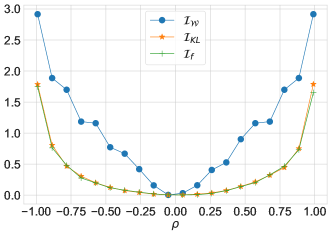
Figure 1: Estimation of different dependency measures for multivariate Gaussian random variables for different degree of correlation.

3 Model and training objective

In this section, we introduce our new set of losses to improve fusion. In sec. 3.1, we first extend widely used bi-variate dependency measures to multivariate dependencies James and Crutchfield (2017) measures (MDM). We then introduce variational bounds on the MDM, and in sec. 3.2, we describe our method to minimise the proposed variational bounds.
Notations We consider $X_{a},X_{v},X_{l}$ as the multimodal data from the audio,video and language modality respectively with joint probability distribution $p_{X_{a}X_{v}X_{l}}$. We denote as $p_{X_{j}}$ the marginal distribution of $X_{j}$ with $j\in\{a,v,l\}$ corresponding to the $j$th modality.
General loss As previously mentioned, we rely on the InfoMax principle Linsker (1988) and aim at jointly maximising the MDM between the different modalities and minimising the task loss; hence, we are in a multi-task setting Argyriou et al. (2007); Ruder (2017) and the objective of interest can be defined as:

$$\mathcal{L}\triangleq\underbrace{\mathcal{L}_{down.}}_{\textrm{main task}}-\underbrace{\lambda\cdot\mathcal{L}_{MDM}}_{\textrm{mutual dependency term}}.$$ (5)

$\mathcal{L}_{down.}$ represents a downstream specific (target task) loss i.e a binary cross-entropy or a $L_{1}$ loss, $\lambda$ is a meta-parameter and $\mathcal{L}_{MDM}$ is the multivariate dependencies measures (see sec. 3.2). Minimisation of our newly defined objectives requires to derive lower bounds on the $\mathcal{L}_{MDM}$ terms, and then to obtain trainable surrogates.

3.1 From bivariate to multivariate dependencies

In our setting, we aim at maximising cross-view interactions involving three modalities, thus we need to generalise bivariate dependency measures to multivariate dependency measures.

Definition 3.1 (Multivariate Dependencies Measures).

Let $X_{a},X_{v},X_{l}$ be a set of random variables with joint pdf $p_{X_{a}X_{v}X_{l}}$ and respective marginal pdf $p_{X_{j}}$ with $j\in\{a,v,l\}$. Then we defined the multivariate mutual information $\textbf{I}_{kl}$ which is also refered as total correlation Watanabe (1960) or multi-information Studenỳ and Vejnarová (1998):

$$\textbf{I}_{kl}\triangleq\mathop{KL}(p_{X_{a}X_{v}X_{l}}(x_{a},x_{v},x_{l})||\prod\limits_{j\in\{a,v,l\}}p_{X_{j}}(x_{j})).$$

Simarly for any f-divergence we define the multivariate f-mutual information $\textbf{I}_{f}$ as:

$$\textbf{I}_{f}\triangleq\mathcal{D}_{f}(p_{X_{a}X_{v}X_{l}}(x_{a},x_{v},x_{l});\prod\limits_{j\in\{a,v,l\}}p_{X_{j}}(x_{j})).$$

Finally, we also extend Eq. 3 to obtain the multivariate Wasserstein dependency measure $\textbf{I}_{\mathcal{W}}$:

$$\textbf{I}_{\mathcal{W}}\triangleq\mathcal{W}(p_{X_{a}X_{v}X_{l}}(x_{a},x_{v},x_{l});\prod\limits_{j\in\{a,v,l\}}p_{X_{j}}(x_{j})).$$

where $\mathcal{W}$ denotes the Wasserstein distance.

3.2 From theoretical bounds to trainable surrogates

To train our neural architecture we need to estimate the previously defined multivariate dependency measures. We rely on neural estimators that are given in Th. 1.

Theorem 1.

Multivariate Neural Dependency Measures Let the family of functions $T(\theta):\mathcal{X}_{a}\times\mathcal{X}_{v}\times\mathcal{X}_{l}\rightarrow\mathbb{R}$ parametrized by a deep neural network with learnable parameters $\theta\in\Theta$. The multivariate mutual information measure $\textbf{I}_{kl}$ is defined as:

$$\textbf{I}_{kl}\triangleq\underset{\theta}{\text{sup}}\quad\mathbb{E}_{p_{X_{a}X_{v}X_{l}}}[T_{\theta}]-\log\big{[}\mathbb{E}_{\prod\limits_{j\in\{a,v,l\}}p_{X_{j}}}[e^{T_{\theta}}]\big{]}.$$ (6)

The neural multivariate f-mutual information measure $\textbf{I}_{f}$ is defined as follows:

$$\textbf{I}_{f}\triangleq\underset{\theta}{\text{sup}}\quad\mathbb{E}_{p_{X_{a}X_{v}X_{l}}}[T_{\theta}]-\mathbb{E}_{\prod\limits_{j\in\{a,v,l\}}p_{X_{j}}}[e^{T_{\theta}-1}].$$ (7)

The neural multivariate Wasserstein dependency measure $\textbf{I}_{\mathcal{W}}$ is defined as follows:

$$\textbf{I}_{\mathcal{W}}\triangleq\underset{\theta:T_{\theta}\in\mathbb{L}}{\text{sup}}\mathbb{E}_{p_{X_{a}X_{v}X_{l}}}[T_{\theta}]-\log\big{[}\mathbb{E}_{\prod\limits_{j\in\{a,v,l\}}p_{X_{j}}}[T_{\theta}]\big{]}.$$ (8)

Where $\mathbb{L}$ is the set of all 1-Lipschitz functions from $\mathcal{R}^{d}\rightarrow\mathcal{R}$

Sketch of proofs: Eq. 6 is a direct application of the Donsker-Varadhan representation of the KL divergence (we assume that the integrability constraints are satisfied). Eq. 7 comes from the work of Nguyen et al. (2017). Eq. 8 comes from the Kantorovich-Rubenstein: we refer the reader to Villani (2008); Peyré et al. (2019) for a rigorous and exhaustive treatment.
Practical estimate of the variational bounds. The empirical estimator that we derive from Th. 1 can be used in practical way: the expectations in Eq. 6, Eq. 7 and Eq. 8 are estimated using empirical samples from the joint distribution $p_{X_{a}X_{v}X_{l}}$. The empirical samples from $\prod\limits_{j\in\{a,v,l\}}p_{X_{j}}$ are obtained by shuffling the samples from the joint distribution in a batch. We integrate this into minimising a multi-task objective (5) by using minus the estimator. We refer to the losses obtained with the penalty based on the estimators described in Eq. 6, Eq. 7 and Eq. 8 as $\mathcal{L}_{kl}$, $\mathcal{L}_{f}$ and $\mathcal{L}_{\mathcal{W}}$ respectively. Details on the practical minimisation of our variational bounds are provided in Algorithm 1.

Remark.

In this work we choose to generalise MINE to compute multivariate dependencies. Comparing our proposed algorithm to other alternatives mentioned in sec. 2 is left for future work. This choice is driven by two main reasons: (1) our framework allows the use of various types of contrast measures (e.g Wasserstein distance,$f$-divergences); (2) the critic network $T_{\theta}$ can be used for interpretability purposes as shown in sec. 5.4.

$\mathcal{D}_{n}=\{(x^{j}_{a},x^{j}_{v},x^{j}_{l}),\forall j\in[1,n]\}$ multimodal training dataset, $m$ batch size, $\sigma_{a},\sigma_{v},\sigma_{l}:[1,m]\rightarrow[1,m]$ three permutations, $\theta_{c}$ weights of the deep classifier, $\theta$ weights of the statistical network $T_{\theta}$.

parameters $\theta$ and $\theta_{c}$

$$\bar{\mathcal{D}_{n}}=\{(x^{\sigma_{a}(j)}_{a},x^{\sigma_{v}(j)}_{v},x^{\sigma_{l}(j)}_{l}),\forall j\in[1,n]\}$$

while $(\theta,\theta_{c})$ not converged do

     for  $i\in[1,Unroll]$ do

         Sample from $\mathcal{D}_{n}$, $\mathcal{B}\sim p_{X_{a}X_{v}X_{l}}$

         Sample from $\bar{\mathcal{D}_{n}}$, $\bar{\mathcal{B}}\sim\prod\limits_{j\in\{a,v,l\}}p_{X_{j}}$

         Update $\theta$ based on the empirical version of Eq. 6 or Eq. 7 or Eq. 8.

     end for

     Sample a batch $\mathcal{B}$ from $\mathcal{D}$

     Update $\theta_{c}$ with $\mathcal{B}$ using Eq. 5.

end while

Classifiers weights ${\theta_{c}}$

Algorithm 1 Two-stage procedure to minimise multivariate dependency measures.

4 Experimental setting

In this section, we present our experimental settings including the neural architectures we compare, the datasets, the metrics and our methodology, which includes the hyper-parameter selection.

4.1 Datasets

We empirically evaluate our methods on two english datasets: CMU-MOSI and CMU-MOSEI. Both datasets have been frequently used to assess model performance in human multimodal sentiment and emotion recognition.
CMU-MOSI: Multimodal Opinion Sentiment Intensity Wöllmer et al. (2013) is a sentiment annotated dataset gathering $2,199$ short monologue video clips.
CMU-MOSEI: CMU-Multimodal Opinion Sentiment and Emotion Intensity Zadeh et al. (2018c) is an emotion and sentiment annotated corpus consisting of $23,454$ movie review videos taken from YouTube. Both CMU-MOSI and CMU-MOSEI are labelled by humans with a sentiment score in $[-3,3]$. For each dataset, three modalities are available; we follow prior work Zadeh et al. (2018b, 2017); Rahman et al. (2020) and the features that have been obtained as follows:
Language: Video transcripts are converted to word embeddings using either Glove Pennington et al. (2014), BERT or XLNET contextualised embeddings. For Glove, the embeddings are of dimension $300$, where for BERT and XLNET this dimension is $768$.
Vision: Vision features are extracted using Facet which results into facial action units corresponding to facial muscle movement. For CMU-MOSEI, the video vectors are composed of $47$ units, and for CMU-MOSI they are composed of $35$.
Audio : Audio features are extracted using COVAREP Degottex et al. (2014). This results into a vector of dimension $74$ which includes $12$ Mel-frequency cepstral coefficients (MFCCs), as well as pitch tracking and voiced/unvoiced segmenting features, peak slope parameters, maxima dispersion quotients and glottal source parameters.
Video and audio are aligned on text-based following the convention introduced in Chen et al. (2017) and the forced alignment described in Yuan and Liberman (2008).

4.2 Evaluation metrics

Multimodal Opinion Sentiment Intensity prediction is treated as a regression problem. Thus, we report both the Mean Absolute Error (MAE) and the correlation of model predictions with true labels. In the literature, the regression task is also turned into a binary classification task for polarity prediction. We follow standard practices Rahman et al. (2020) and report the Accuracy ($Acc_{7}$ denotes accuracy on 7 classes and $Acc_{2}$ the binary accuracy) of our best performing models.

4.3 Neural architectures

In our experiments, we choose to modify the loss function of the different models that have been introduced for multi-modal sentiment analysis on both CMU-MOSI and CMU-MOSEI: Memory Fusion Network (MFN Zadeh et al. (2018a)), Low-rank Multimodal Fusion (LFN Liu et al. (2018)) and two state-of-the-art transformers based models Rahman et al. (2020) for fusion rely on BERT Devlin et al. (2018) (MAG-BERT) and XLNET Yang et al. (2019) (MAG-XLNT). To assess the validity of the proposed losses, we also apply our method to a simple early fusion LSTM (EF-LSTM) as a baseline model.
Model overview: Aforementioned models can be seen as a multi-modal encoder $f_{\theta_{e}}$ providing a representation $Z_{avl}$ containing information and dependencies between modalities $X_{l},X_{a},X_{v}$ namely:

$$f_{\theta_{e}}(X_{a},X_{v},X_{l}) =Z_{avl}.$$

As a final step, a linear transformation $A_{\theta_{p}}$ is applied to $Z_{avl}$ to perform the regression.

EF-LSTM: is the most basic architecture used in the current multimodal analysis where each sequence view is encoded separately with LSTM channels. Then, a fusion function is applied to all representations.
TFN: computes a representation of each view, and then applies a fusion operator. Acoustic and visual views are first mean-pooled then encoded through a 2-layers perceptron. Linguistic features are computed with a LSTM channel. Here, the fusion function is a cross-modal product capturing unimodal, bimodal and trimodal interactions across modalities.
MFN enriches the previous EF-LSTM architecture with an attention module that computes a cross-view representation at each time step. They are then gathered and a final representation is computed by a gated multi-view memory Zadeh et al. (2018a).
MAG-BERT and MAG-XLNT are based on pre-trained transformer architectures Devlin et al. (2018); Yang et al. (2019) allowing inputs on each of the transformer units to be multimodal, thanks to a special gate inspired by Wang et al. (2018). The $Z_{avl}$ is the $[CLS]$ representation provided by the last transformer head. For each architecture, we use the optimal architecture hyperparameters provided by the associated papers (see sec. 8).

5 Numerical results

We present and discuss here the results obtained using the experimental setting described in sec. 4. To better understand the impact of our new methods, we propose to investigate the following points:
Efficiency of the $\mathcal{L}_{MDM}$: to gain understanding of the usefulness of our new objectives, we study the impact of adding the mutual dependency term on the basic multimodal neural model EF-LSTM.
Improving model performance and comparing multivariate dependency measures: the choice of the most suitable dependency measure for a given task is still an open problem (see sec. 3). Thus, we compare the performance – on both multimodal sentiment and emotion prediction tasks– of the different dependency measures. The compared measures are combined with different models using various fusion mechanisms.
Improving the robustness to modality drop: a desirable quality of multimodal representations is the robustness to a missing modality. We study how the maximisation of mutual dependency measures during training affects the robustness of the representation when a modality becomes missing.
Towards explainable representations: the statistical network $T_{\theta}$ allows us to compute a dependency measure between the three considered modalities. We carry out a qualitative analysis in order to investigate if a high dependency can be explained by complementariness across modalities.

5.1 Efficiency of the MDM penalty

For a simple EF-LSTM, we study the improvement induced by addition of our MDM penalty. The results are presented in Tab. 1, where a EF-LSTM trained with no mutual dependency term is denoted with $\mathcal{L}_{\emptyset}$. On both studied datasets, we observe that the addition of a MDM penalty leads to stronger performances on all metrics. For both datasets, we observe that the best performing models are obtained by training with an additional mutual dependency measure term. Keeping in mind the example shown in Fig. 1, we can draw a first comparison between the different dependency measures. Although in a simple case $\mathcal{L}_{f}$ and $\mathcal{L}_{kl}$ estimate a similar quantity (see Fig. 1), in more complex practical applications they do not achieve the same performance. Even though, the Donsker-Varadhan bound used for $\mathcal{L}_{kl}$ is stronger than the one used to estimate $\mathcal{L}_{f}$; for a simple model the stronger bound does not lead to better results. It is possible that most of the differences in performance observed come from the optimisation process during training.
Takeaways: On the simple case of EF-LSTM adding MDM penalty improves the performance on the downstream tasks.

	$Acc^{h}_{7}$	$Acc^{h}_{2}$	$MAE^{l}$	$Corr^{h}$
CMU-MOSI
$\mathcal{L}_{\emptyset}$	31.1	76.1	1.00	0.65
$\mathcal{L}_{kl}$	31.7	76.4	1.00	0.66
$\mathcal{L}_{f}$	33.7	76.2	1.02	0.66
$\mathcal{L}_{\mathcal{W}}$	33.5	76.4	0.98	0.66
CMU-MOSEI
$\mathcal{L}_{\emptyset}$	44.2	75.0	0.72	0.52
$\mathcal{L}_{kl}$	44.5	75.6	0.70	0.53
$\mathcal{L}_{f}$	45.5	75.2	0.70	0.52
$\mathcal{L}_{\mathcal{W}}$	45.3	75.9	0.68	0.54

Table 1: Results on sentiment analysis on both CMU-MOSI and CMU-MOSEI for a EF-LSTM. $Acc_{7}$ denotes accuracy on 7 classes and $Acc_{2}$ the binary accuracy. $MAE$ denotes the Mean Absolute Error and $Corr$ is the Pearson correlation. ^h means higher is better and ^l means lower is better. The choice of the evaluation metrics follows standard practices Rahman et al. (2020). Underline results demonstrate significant improvement (p-value belows 0.05) against the baseline when performing the Wilcoxon Mann Whitney test Wilcoxon (1992) on 10 runs using different seeds.

5.2 Improving models and comparing multivariate dependency measures

In this experiment, we apply the different penalties to more advanced architectures, using various fusion mechanisms.
General analysis. Tab. 2 shows the performance of various neural architectures trained with and without MDM penalty. Results are coherent with the previous experiment: we observe that jointly maximising a mutual dependency measure leads to better results on the downstream task: for example, a MFN on CMU-MOSI trained with $\mathcal{L}_{\mathcal{W}}$ outperforms by $4.6$ points on $Acc^{h}_{7}$ the model trained without the mutual dependency term. On CMU-MOSEI we also obtain subsequent improvements while training with MMD. On CMU-MOSI the TFN also strongly benefits from the mutual dependency term with an absolute improvement of $3.7\%$ (on $Acc^{h}_{7}$) with $\mathcal{L}_{\mathcal{W}}$ compared to $\mathcal{L}_{\emptyset}$. Tab. 2 shows that our methods not only perform well on recurrent architectures but also on pretrained Transformer-based models, that achieve higher results due to a superior capacity to model contextual dependencies (see Rahman et al. (2020)).
Improving state-of-the-art models. MAGBERT and MAGXLNET are state-of-the art models on both CMU-MOSI and CMU-MOSEI. From Tab. 2, we observe that our methods can improve the performance of both models. It is worth noting that, in both cases, $\mathcal{L}_{\mathcal{W}}$ combined with pre-trained transformers achieves good results. This performance gain suggests that our method is able to capture dependencies that are not learnt during either pretraining of the language model (i.e BERT or XLNET) or by the Multimodal Adaptation Gate used to perform the fusion.
Comparing dependency measures. Tab. 2 shows that there is no dependency measure that achieves the best results in all cases. This result tends to confirm that the optimisation process during training plays an important role (see hypothesis in sec. 5.1). However, we can observe that optimising the multivariate Wasserstein dependency measure is usually a good choice, since it achieves state of the art results in many configurations. It is worth noting that several pieces of research point the limitations of mutual information estimators McAllester and Stratos (2020); Song and Ermon (2019).
Takeaways: The addition of MMD not only benefits simple models (e.g EF-LSTM) but also improves performance when combined with both complex fusion mechanisms and pretrained models. For practical applications, the Wasserstein distance is a good choice of contrast function.

	CMU-MOSI				CMU-MOSEI
	$Acc^{h}_{7}$	$Acc^{h}_{2}$	$MAE^{l}$	$Corr^{h}$	$Acc^{h}_{7}$	$Acc^{h}_{2}$	$MAE^{l}$	$Corr^{h}$
MFN
$\mathcal{L}_{\emptyset}$	31.3	76.6	1.01	0.62	44.4	74.7	0.72	0.53
$\mathcal{L}_{kl}$	32.5	76.7	0.96	0.65	44.2	74.7	0.72	0.57
$\mathcal{L}_{f}$	35.7	77.4	0.96	0.65	46.1	75.4	0.69	0.56
$\mathcal{L}_{\mathcal{W}}$	35.9	77.6	0.96	0.65	46.2	75.1	0.69	0.56
LFN
$\mathcal{L}_{\emptyset}$	31.9	76.9	1.00	0.63	45.2	74.2	0.70	0.54
$\mathcal{L}_{kl}$	32.6	77.7	0.97	0.63	46.1	75.3	0.68	0.57
$\mathcal{L}_{f}$	35.6	77.1	0.97	0.63	45.8	75.4	0.69	0.57
$\mathcal{L}_{\mathcal{W}}$	35.6	77.7	0.96	0.67	46.2	75.4	0.67	0.57
MAGBERT
$\mathcal{L}_{\emptyset}$	40.2	84.7	0.79	0.80	46.8	84.9	0.59	0.77
$\mathcal{L}_{kl}$	42.0	85.6	0.76	0.82	47.1	85.4	0.59	0.79
$\mathcal{L}_{f}$	41.7	85.6	0.78	0.82	46.9	85.6	0.59	0.79
$\mathcal{L}_{\mathcal{W}}$	41.8	85.3	0.76	0.82	47.8	85.5	0.59	0.79
MAGXLNET
$\mathcal{L}_{\emptyset}$	43.0	86.2	0.76	0.82	46.7	84.4	0.59	0.79
$\mathcal{L}_{kl}$	44.5	86.1	0.74	0.82	47.5	85.4	0.59	0.81
$\mathcal{L}_{f}$	43.9	86.6	0.74	0.82	47.4	85.0	0.59	0.81
$\mathcal{L}_{\mathcal{W}}$	44.4	86.9	0.74	0.82	47.9	85.8	0.59	0.82

Table 2: Results on sentiment and emotion prediction on both CMU-MOSI and CMU-MOSEI dataset for the different neural architectures presented in sec. 4 relying on various fusion mechanisms.

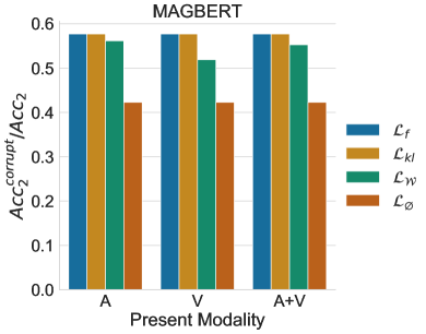
Figure 2: Study of the robustness of the representations against drop of the linguistic modality. Studied model is MAGBERT on CMU-MOSI. The ratio between the accuracy achieved with a corrupted linguistic modality $Acc_{2}^{corrupt}$ and the accuracy $Acc_{2}$ without any corruption is reported on $y$-axis. The preserved modalities during inference are reported on $x$-axis. $A$, $V$ respectively stands for acoustic and visual modality.

Spoken Transcripts	Acoustic and visual behaviour	$T_{\theta}$
um the story was all right	low energy monotonous voice + headshake	L
i mean its a Nicholas Sparks book it must be good	disappointed tone + neutral facial expression	L
the action is fucking awesome	head nod + excited voice	H
it was cute you know the actors did a great job bringing the smurfs to life such as joe george lopez neil patrick harris katy perry and a fourth	multiple smiles	H

Table 3: Examples from the CMU-MOSI dataset using MAGBERT. The last column is computed using the statistical network $T_{\theta}$. $L$ stands for low values and $H$ stands for high values. Green, grey, red highlight positive, neutral and negative expression/behaviours respectively

5.3 Improved robustness to modality drop

Although fusion with visual and acoustic modalities provided a performance improvement Wang et al. (2018), the performance of Multimodal systems on sentiment prediction tasks is mainly carried by the linguistic modality Zadeh et al. (2018a, 2017). Thus it is interesting to study how a multimodal system behaves when the text modality is missing because it gives insights on the robustness of the representation.
Experiment description. In this experiment, we focus on the MAGBERT and MAGXLNET since they are the best performing models. As before, the considered models are trained using the losses described in sec. 3 and all modalities are kept during training time. During inference, we either keep only one modality (Audio or Video) or both. Text modality is always dropped.
Results. Results of the experiments conducted on CMU-MOSI are shown in Fig. 2, giving values for the ratio $Acc_{2}^{corrupt}/Acc_{2}$ where $Acc_{2}^{corrupt}$ is the binary accuracy in the corrupted configuration and $Acc_{2}$ the accuracy obtained when all modalities are considered. We observe that models trained with an MDM penalty (either $\mathcal{L}_{kl}$, $\mathcal{L}_{f}$ or $\mathcal{L}_{\mathcal{W}}$) resist better to missing modalities than those trained with $\mathcal{L}_{\emptyset}$. For example, when trained with $\mathcal{L}_{kl}$ or $\mathcal{L}_{f}$, the drop in performance is limited to $\approx 25\%$ in any setting. Interestingly, for MAGBERT $\mathcal{L}_{\mathcal{W}}$ and $\mathcal{L}_{KL}$ achieve comparable results; $\mathcal{L}_{KL}$ is more resistant to dropping the language modality, and thus, could be preferred in practical applications.
Takeaway: Maximising the MMD allows an information transfer between modalities.

5.4 Towards explainable representations

In this section, we propose a qualitative experiment allowing us to interpret the predictions made by the deep neural classifier. During training, $T_{\theta}$ estimates the mutual dependency measure, using the surrogates introduced in Th. 1. However, the inference process only involves the classifier, and $T_{\theta}$ is unused. Eq. 6, Eq. 7, Eq. 8 show that $T_{\theta}$ is trained to discriminate between valid representations (coming from the joint distribution) and corrupted representations (coming from the product of the marginals). Thus, $T_{\theta}$ can be used, at inference time, to measure the mutual dependency of the representations used by the neural model. In Tab. 3 we report examples of low and high discrepancy measures for MAGBERT on CMU-MOSI. We can observe that high values correspond to video clips where audio, text and video are complementary (e.g use of head node McClave (2000)) and low values correspond to the case where there exists contradictions across several modalities. Results on MAGXLET can be found in sec. 8.3.
Takeaways: $T_{\theta}$ used to estimate the MDM provides a mean to interpret representations learnt by the encoder.

6 Conclusions

In this paper, we introduced three new losses based on MDM. Through extensive set of experiments on CMU-MOSI and CMU-MOSEI, we have shown that SOTA architectures can benefit from these innovations with little modifications. A by-product of our method involves a statistical network that is a useful tool to explain the learnt high dimensional multi-modal representations. This work paves the way for using and developing new alternative methods to improve the learning (e.g new estimator of mutual information Colombo et al. (2021a), Wasserstein Barycenters Colombo et al. (2021b), Data Depths Staerman et al. (2021), Extreme Value Theory Jalalzai et al. (2020)). A future line of research involves using this methods for emotion Colombo et al. (2019); Witon et al. (2018) and dialog act Chapuis et al. (2021, 2020a, 2020b) classification with pre-trained model tailored for spoken language Dinkar et al. (2020).

7 Acknowledgments

The research carried out in this paper has received funding from IBM, the French National Research Agency’s grant ANR-17-MAOI and the DSAIDIS chair at Telecom-Paris. This work was also granted access to the HPC resources of IDRIS under the allocation 2021-AP010611665 as well as under the project 2021-101838 made by GENCI.

8 Supplementary

8.1 Training details

In this section, we both present a comprehensive illustration of the Algorithm 1 and state the details of experimental hyperparameters selection as well as and the architectures used for the statistic network $T_{\theta}$.

8.1.1 Illustration of Algorithm 1

Fig. 3 describes the Algorithm 1. As can be seen in the figure, to compute the mutual dependency measure the statistic network $T_{\theta}$ takes the two embeddings of the different batch $\mathcal{B}$ and $\bar{\mathcal{B}}$.

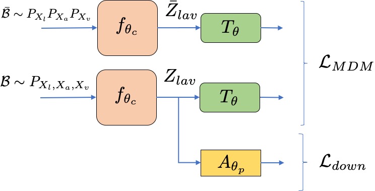
Figure 3: Illustration of the method describes in Algorithm 1 for the different estimators derived from Th. 1. $\mathcal{B}$ and $\bar{\mathcal{B}}$ stands for the batch of data sample from the joint probability distribution and the product of the marginal distribution respectively. $Z_{avl}$ denotes the fusion representation of linguistic, acoustic and visual (resp. $l$, $a$ and $v$) modalities provided by a multimodal architecture $f_{\theta_{e}}$ for the batch $\mathcal{B}$ . $\overline{Z}_{lav}$ denotes the same quantity as described before for the batch $\bar{\mathcal{B}}$. $A_{\theta_{p}}$ denotes the linear projection before classification or regression.

8.1.2 Hyperparameters selection

We use dropout Srivastava et al. (2014) and optimise the global loss Eq. 5 by gradient descent using AdamW Loshchilov and Hutter (2017); Kingma and Ba (2014) optimiser. The best learning rate is found in the grid $\{0.002,0.001,0.0005,0.0001\}$. The best model is selected using the lowest MAE on the validation set. We $Unroll$ to 10.

8.1.3 Architectures of $T_{\theta}$

Across the different experiment we use a statistic network with an architecture as describes in Tab. 4. We follow Belghazi et al. (2018) and use LeakyRELU Agarap (2018); Xu et al. (2015) as activation function.

Statistic Network
Layer	Number of outputs	Activation function
$[Z_{lav},\overline{Z}_{lav}]$	$d_{in},d_{in}$	-
Dense layer	$d_{in}/2$	LeakyReLU
Dropout	0.4	-
Dense layer	$d_{in}$	LeakyReLU
Dropout	0.4	-
Dense layer	$d_{in}$	LeakyReLU
Dropout	0.4	-
Dense layer	$d_{in}/4$	LeakyReLU
Dropout	0.4	-
Dense layer	$d_{in}/4$	LeakyReLU
Dropout	0.4	-
Dense layer	1	Sigmoïd

Table 4: Statistics network description. $d_{in}$ denotes the dimension of $Z_{avl}$.

8.2 Additional experiments for robustness to modality drop

Fig. 4 shows the results of the robustness text on MAGXLNET. Similarly to Fig. 2 we observe more robust representation to modality drop when jointly maximising the $\mathcal{L}_{\mathcal{W}}$ and $\mathcal{L}_{kl}$ with the target loss. Fig. 4 shows no improvement when training with $\mathcal{L}_{f}$. This can also be linked to Tab. 2 which similarly shows no improvement in this very specific configuration.

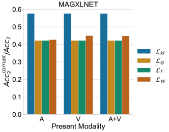
Figure 4: Study of the robustness of the representations against a drop of the linguistic modality. Studied model is MAGXLNET on CMU-MOSI. The ratio between the accuracy achieved with a corrupted linguistic modality $Acc_{2}^{corrupt}$ and the accuracy $Acc_{2}$ without any corruption is reported on $y$-axis. The preserved modalities during inference are reported on $x$-axis. $A$, $V$ respectively stands for the acoustic and visual modality.

8.3 Additional qualitative examples

Tab. 5 illustrates the use of $T_{\theta}$ to explain the representations learnt by the model. Similarly to Tab. 4 we observe that high values correspond to complementarity across modalities and low values are related to contradictoriness across modalities.

Spoken Transcripts	Acoustic and visual behaviour	$T_{\theta}$
but the m the script is corny	high energy voice + headshake + (many) smiles	L
as for gi joe was it was just like laughing its the the plot the the acting is terrible	high enery voice + laughts + smiles	L
but i think this one did beat scream 2 now	headshake + long sigh	L
the xxx sequence is really well done	static head + low energy monotonous voice	L
you know of course i was waithing for the princess and the frog	smiles + high energy voice + + high pitch	H
dennis quaid i think had a lot of fun	smiles + high energy voice	H
it was very very very boring	low energy voice + frown eyebrows	H
i do not wanna see any more of this	angry voice + angry facial expression	H

Table 5: Examples from the CMU-MOSI dataset using MAGXLNET trained with $\mathcal{L}_{\mathcal{W}}$. The last column is computed using the statistic network $T_{\theta}$. $L$ stands for low values and $H$ stands for high values. Green, grey, red highlight positive, neutral and negative expression/behaviours respectively.

References

- Agarap (2018) Abien Fred Agarap. 2018. Deep learning using rectified linear units (relu). arXiv preprint arXiv:1803.08375.
- Argyriou et al. (2007) Andreas Argyriou, Theodoros Evgeniou, and Massimiliano Pontil. 2007. Multi-task feature learning. In Advances in neural information processing systems, pages 41–48.
- Baltrušaitis et al. (2018) Tadas Baltrušaitis, Chaitanya Ahuja, and Louis-Philippe Morency. 2018. Multimodal machine learning: A survey and taxonomy. IEEE transactions on pattern analysis and machine intelligence, 41(2):423–443.
- Belghazi et al. (2018) Mohamed Ishmael Belghazi, Aristide Baratin, Sai Rajeswar, Sherjil Ozair, Yoshua Bengio, Aaron Courville, and R Devon Hjelm. 2018. Mine: mutual information neural estimation. arXiv preprint arXiv:1801.04062.
- Boudiaf et al. (2020) Malik Boudiaf, Jérôme Rony, Imtiaz Masud Ziko, Eric Granger, Marco Pedersoli, Pablo Piantanida, and Ismail Ben Ayed. 2020. A unifying mutual information view of metric learning: cross-entropy vs. pairwise losses. In European Conference on Computer Vision, pages 548–564. Springer.
- Busso et al. (2008) Carlos Busso, Murtaza Bulut, Chi-Chun Lee, Abe Kazemzadeh, Emily Mower, Samuel Kim, Jeannette N Chang, Sungbok Lee, and Shrikanth S Narayanan. 2008. Iemocap: Interactive emotional dyadic motion capture database. Language resources and evaluation, 42(4):335.
- Chapuis et al. (2021) Emile Chapuis, Pierre Colombo, Matthieu Labeau, and Chloé Clave. 2021. Code-switched inspired losses for generic spoken dialog representations. CoRR, abs/2108.12465.
- Chapuis et al. (2020a) Emile Chapuis, Pierre Colombo, Matteo Manica, Matthieu Labeau, and Chloé Clavel. 2020a. Hierarchical pre-training for sequence labelling in spoken dialog. CoRR, abs/2009.11152.
- Chapuis et al. (2020b) Emile Chapuis, Pierre Colombo, Matteo Manica, Matthieu Labeau, and Chloé Clavel. 2020b. Hierarchical pre-training for sequence labelling in spoken dialog. In Findings of the Association for Computational Linguistics: EMNLP 2020, Online Event, 16-20 November 2020, volume EMNLP 2020 of Findings of ACL, pages 2636–2648. Association for Computational Linguistics.
- Chen et al. (2017) Minghai Chen, Sen Wang, Paul Pu Liang, Tadas Baltrušaitis, Amir Zadeh, and Louis-Philippe Morency. 2017. Multimodal sentiment analysis with word-level fusion and reinforcement learning. In Proceedings of the 19th ACM International Conference on Multimodal Interaction, pages 163–171.
- Colombo et al. (2021a) Pierre Colombo, Chloé Clavel, and Pablo Piantanida. 2021a. A novel estimator of mutual information for learning to disentangle textual representations. CoRR, abs/2105.02685.
- Colombo et al. (2021b) Pierre Colombo, Guillaume Staerman, Chloé Clavel, and Pablo Piantanida. 2021b. Automatic text evaluation through the lens of wasserstein barycenters. CoRR, abs/2108.12463.
- Colombo et al. (2019) Pierre Colombo, Wojciech Witon, Ashutosh Modi, James Kennedy, and Mubbasir Kapadia. 2019. Affect-driven dialog generation. In Proceedings of the 2019 Conference of the North American Chapter of the Association for Computational Linguistics: Human Language Technologies, NAACL-HLT 2019, Minneapolis, MN, USA, June 2-7, 2019, Volume 1 (Long and Short Papers), pages 3734–3743. Association for Computational Linguistics.
- Degottex et al. (2014) Gilles Degottex, John Kane, Thomas Drugman, Tuomo Raitio, and Stefan Scherer. 2014. Covarep—a collaborative voice analysis repository for speech technologies. In 2014 ieee international conference on acoustics, speech and signal processing (icassp), pages 960–964. IEEE.
- Devlin et al. (2018) Jacob Devlin, Ming-Wei Chang, Kenton Lee, and Kristina Toutanova. 2018. Bert: Pre-training of deep bidirectional transformers for language understanding. arXiv preprint arXiv:1810.04805.
- Dilpazir et al. (2016) Hammad Dilpazir, Zia Muhammad, Qurratulain Minhas, Faheem Ahmed, Hafiz Malik, and Hasan Mahmood. 2016. Multivariate mutual information for audio video fusion. Signal, Image and Video Processing, 10(7):1265–1272.
- Dinkar et al. (2020) Tanvi Dinkar, Pierre Colombo, Matthieu Labeau, and Chloé Clavel. 2020. The importance of fillers for text representations of speech transcripts. In Proceedings of the 2020 Conference on Empirical Methods in Natural Language Processing, EMNLP 2020, Online, November 16-20, 2020, pages 7985–7993. Association for Computational Linguistics.
- Donsker and Varadhan (1985) MD Donsker and SRS Varadhan. 1985. Large deviations for stationary gaussian processes. Communications in Mathematical Physics, 97(1-2):187–210.
- Garcia et al. (2019a) Alexandre Garcia, Pierre Colombo, Slim Essid, Florence d’Alché Buc, and Chloé Clavel. 2019a. From the token to the review: A hierarchical multimodal approach to opinion mining. arXiv preprint arXiv:1908.11216.
- Garcia et al. (2019b) Alexandre Garcia, Slim Essid, Florence d’Alché Buc, and Chloé Clavel. 2019b. A multimodal movie review corpus for fine-grained opinion mining. arXiv preprint arXiv:1902.10102.
- Hazarika et al. (2020) Devamanyu Hazarika, Roger Zimmermann, and Soujanya Poria. 2020. Misa: Modality-invariant and-specific representations for multimodal sentiment analysis. arXiv preprint arXiv:2005.03545.
- Hjelm et al. (2018) R Devon Hjelm, Alex Fedorov, Samuel Lavoie-Marchildon, Karan Grewal, Phil Bachman, Adam Trischler, and Yoshua Bengio. 2018. Learning deep representations by mutual information estimation and maximization. arXiv preprint arXiv:1808.06670.
- Huang et al. (2015) Zhiheng Huang, Wei Xu, and Kai Yu. 2015. Bidirectional lstm-crf models for sequence tagging. arXiv preprint arXiv:1508.01991.
- Jalalzai et al. (2020) Hamid Jalalzai, Pierre Colombo, Chloé Clavel, Éric Gaussier, Giovanna Varni, Emmanuel Vignon, and Anne Sabourin. 2020. Heavy-tailed representations, text polarity classification & data augmentation. In Advances in Neural Information Processing Systems 33: Annual Conference on Neural Information Processing Systems 2020, NeurIPS 2020, December 6-12, 2020, virtual.
- James and Crutchfield (2017) Ryan G James and James P Crutchfield. 2017. Multivariate dependence beyond shannon information. Entropy, 19(10):531.
- Khan et al. (2012) Fahad Shahbaz Khan, Rao Muhammad Anwer, Joost Van De Weijer, Andrew D Bagdanov, Maria Vanrell, and Antonio M Lopez. 2012. Color attributes for object detection. In 2012 IEEE Conference on Computer Vision and Pattern Recognition, pages 3306–3313. IEEE.
- Kingma and Ba (2014) Diederik P Kingma and Jimmy Ba. 2014. Adam: A method for stochastic optimization. arXiv preprint arXiv:1412.6980.
- Kinney and Atwal (2014) Justin B Kinney and Gurinder S Atwal. 2014. Equitability, mutual information, and the maximal information coefficient. Proceedings of the National Academy of Sciences, 111(9):3354–3359.
- Kong et al. (2019) Lingpeng Kong, Cyprien de Masson d’Autume, Wang Ling, Lei Yu, Zihang Dai, and Dani Yogatama. 2019. A mutual information maximization perspective of language representation learning. arXiv preprint arXiv:1910.08350.
- Linsker (1988) Ralph Linsker. 1988. Self-organization in a perceptual network. Computer, 21(3):105–117.
- Liu et al. (2018) Zhun Liu, Ying Shen, Varun Bharadhwaj Lakshminarasimhan, Paul Pu Liang, Amir Zadeh, and Louis-Philippe Morency. 2018. Efficient low-rank multimodal fusion with modality-specific factors. arXiv preprint arXiv:1806.00064.
- Loshchilov and Hutter (2017) Ilya Loshchilov and Frank Hutter. 2017. Decoupled weight decay regularization. arXiv preprint arXiv:1711.05101.
- Mai et al. (2019) Sijie Mai, Haifeng Hu, and Songlong Xing. 2019. Divide, conquer and combine: Hierarchical feature fusion network with local and global perspectives for multimodal affective computing. In Proceedings of the 57th Annual Meeting of the Association for Computational Linguistics, pages 481–492.
- McAllester and Stratos (2020) David McAllester and Karl Stratos. 2020. Formal limitations on the measurement of mutual information. In International Conference on Artificial Intelligence and Statistics, pages 875–884.
- McClave (2000) Evelyn Z McClave. 2000. Linguistic functions of head movements in the context of speech. Journal of pragmatics, 32(7):855–878.
- Nguyen et al. (2017) Tu Nguyen, Trung Le, Hung Vu, and Dinh Phung. 2017. Dual discriminator generative adversarial nets. In Advances in Neural Information Processing Systems, pages 2670–2680.
- Nguyen et al. (2010) XuanLong Nguyen, Martin J Wainwright, and Michael I Jordan. 2010. Estimating divergence functionals and the likelihood ratio by convex risk minimization. IEEE Transactions on Information Theory, 56(11):5847–5861.
- Oord et al. (2018) Aaron van den Oord, Yazhe Li, and Oriol Vinyals. 2018. Representation learning with contrastive predictive coding. arXiv preprint arXiv:1807.03748.
- Ozair et al. (2019) Sherjil Ozair, Corey Lynch, Yoshua Bengio, Aaron Van den Oord, Sergey Levine, and Pierre Sermanet. 2019. Wasserstein dependency measure for representation learning. In Advances in Neural Information Processing Systems, pages 15604–15614.
- Park et al. (2014) Sunghyun Park, Han Suk Shim, Moitreya Chatterjee, Kenji Sagae, and Louis-Philippe Morency. 2014. Computational analysis of persuasiveness in social multimedia: A novel dataset and multimodal prediction approach. In Proceedings of the 16th International Conference on Multimodal Interaction, pages 50–57.
- Pennington et al. (2014) Jeffrey Pennington, Richard Socher, and Christopher D Manning. 2014. Glove: Global vectors for word representation. In EMNLP, volume 14, pages 1532–1543.
- Peyré et al. (2019) Gabriel Peyré, Marco Cuturi, et al. 2019. Computational optimal transport: With applications to data science. Foundations and Trends® in Machine Learning, 11(5-6):355–607.
- Pham et al. (2019) Hai Pham, Paul Pu Liang, Thomas Manzini, Louis-Philippe Morency, and Barnabás Póczos. 2019. Found in translation: Learning robust joint representations by cyclic translations between modalities. In Proceedings of the AAAI Conference on Artificial Intelligence, volume 33, pages 6892–6899.
- Rahman et al. (2020) Wasifur Rahman, Md Kamrul Hasan, Sangwu Lee, AmirAli Bagher Zadeh, Chengfeng Mao, Louis-Philippe Morency, and Ehsan Hoque. 2020. Integrating multimodal information in large pretrained transformers. In Proceedings of the 58th Annual Meeting of the Association for Computational Linguistics, pages 2359–2369.
- Ruder (2017) Sebastian Ruder. 2017. An overview of multi-task learning in deep neural networks. arXiv preprint arXiv:1706.05098.
- Siriwardhana et al. (2020) Shamane Siriwardhana, Andrew Reis, Rivindu Weerasekera, and Suranga Nanayakkara. 2020. Jointly fine-tuning" bert-like" self supervised models to improve multimodal speech emotion recognition. arXiv preprint arXiv:2008.06682.
- Soleymani et al. (2017) Mohammad Soleymani, David Garcia, Brendan Jou, Björn Schuller, Shih-Fu Chang, and Maja Pantic. 2017. A survey of multimodal sentiment analysis. Image and Vision Computing, 65:3–14.
- Song and Ermon (2019) Jiaming Song and Stefano Ermon. 2019. Understanding the limitations of variational mutual information estimators. arXiv preprint arXiv:1910.06222.
- Srivastava et al. (2014) Nitish Srivastava, Geoffrey Hinton, Alex Krizhevsky, Ilya Sutskever, and Ruslan Salakhutdinov. 2014. Dropout: a simple way to prevent neural networks from overfitting. The journal of machine learning research, 15(1):1929–1958.
- Staerman et al. (2021) Guillaume Staerman, Pavlo Mozharovskyi, and Stéphan Clémençon. 2021. Affine-invariant integrated rank-weighted depth: Definition, properties and finite sample analysis. arXiv preprint arXiv:2106.11068.
- Studenỳ and Vejnarová (1998) Milan Studenỳ and Jirina Vejnarová. 1998. The multiinformation function as a tool for measuring stochastic dependence. In Learning in graphical models, pages 261–297. Springer.
- Sun et al. (2020) Zhongkai Sun, Prathusha Sarma, William Sethares, and Yingyu Liang. 2020. Learning relationships between text, audio, and video via deep canonical correlation for multimodal language analysis. In Proceedings of the AAAI Conference on Artificial Intelligence, volume 34, pages 8992–8999.
- Tian et al. (2019) Yonglong Tian, Dilip Krishnan, and Phillip Isola. 2019. Contrastive multiview coding. arXiv preprint arXiv:1906.05849.
- Tsai et al. (2019) Yao-Hung Hubert Tsai, Shaojie Bai, Paul Pu Liang, J Zico Kolter, Louis-Philippe Morency, and Ruslan Salakhutdinov. 2019. Multimodal transformer for unaligned multimodal language sequences. In Proceedings of the conference. Association for Computational Linguistics. Meeting, volume 2019, page 6558. NIH Public Access.
- Villani (2008) Cédric Villani. 2008. Optimal transport: old and new, volume 338. Springer Science & Business Media.
- Wang et al. (2018) Yansen Wang, Ying Shen, Zhun Liu, Paul Pu Liang, Amir Zadeh, and Louis-Philippe Morency. 2018. Words can shift: Dynamically adjusting word representations using nonverbal behaviors.
- Watanabe (1960) Satosi Watanabe. 1960. Information theoretical analysis of multivariate correlation. IBM Journal of research and development, 4(1):66–82.
- Wilcoxon (1992) Frank Wilcoxon. 1992. Individual comparisons by ranking methods. In Breakthroughs in statistics, pages 196–202. Springer.
- Witon et al. (2018) Wojciech Witon, Pierre Colombo, Ashutosh Modi, and Mubbasir Kapadia. 2018. Disney at IEST 2018: Predicting emotions using an ensemble. In Proceedings of the 9th Workshop on Computational Approaches to Subjectivity, Sentiment and Social Media Analysis, WASSA@EMNLP 2018, Brussels, Belgium, October 31, 2018, pages 248–253. Association for Computational Linguistics.
- Wöllmer et al. (2013) Martin Wöllmer, Felix Weninger, Tobias Knaup, Björn Schuller, Congkai Sun, Kenji Sagae, and Louis-Philippe Morency. 2013. Youtube movie reviews: Sentiment analysis in an audio-visual context. IEEE Intelligent Systems, 28(3):46–53.
- Xu et al. (2015) Bing Xu, Naiyan Wang, Tianqi Chen, and Mu Li. 2015. Empirical evaluation of rectified activations in convolutional network.
- Xu et al. (2013) Chang Xu, Dacheng Tao, and Chao Xu. 2013. A survey on multi-view learning. arXiv preprint arXiv:1304.5634.
- Yang et al. (2019) Zhilin Yang, Zihang Dai, Yiming Yang, Jaime Carbonell, Russ R Salakhutdinov, and Quoc V Le. 2019. Xlnet: Generalized autoregressive pretraining for language understanding. In Advances in neural information processing systems, pages 5753–5763.
- Ye et al. (2017) Jun Ye, Hao Hu, Guo-Jun Qi, and Kien A Hua. 2017. A temporal order modeling approach to human action recognition from multimodal sensor data. ACM Transactions on Multimedia Computing, Communications, and Applications (TOMM), 13(2):1–22.
- Yuan and Liberman (2008) Jiahong Yuan and Mark Liberman. 2008. Speaker identification on the scotus corpus. Journal of the Acoustical Society of America, 123(5):3878.
- Zadeh et al. (2017) Amir Zadeh, Minghai Chen, Soujanya Poria, Erik Cambria, and Louis-Philippe Morency. 2017. Tensor fusion network for multimodal sentiment analysis. arXiv preprint arXiv:1707.07250.
- Zadeh et al. (2018a) Amir Zadeh, Paul Pu Liang, Navonil Mazumder, Soujanya Poria, Erik Cambria, and Louis-Philippe Morency. 2018a. Memory fusion network for multi-view sequential learning. arXiv preprint arXiv:1802.00927.
- Zadeh et al. (2018b) Amir Zadeh, Paul Pu Liang, Soujanya Poria, Prateek Vij, Erik Cambria, and Louis-Philippe Morency. 2018b. Multi-attention recurrent network for human communication comprehension. In Proceedings of the… AAAI Conference on Artificial Intelligence. AAAI Conference on Artificial Intelligence, volume 2018, page 5642. NIH Public Access.
- Zadeh et al. (2019) Amir Zadeh, Chengfeng Mao, Kelly Shi, Yiwei Zhang, Paul Pu Liang, Soujanya Poria, and Louis-Philippe Morency. 2019. Factorized multimodal transformer for multimodal sequential learning. arXiv preprint arXiv:1911.09826.
- Zadeh et al. (2018c) AmirAli Bagher Zadeh, Paul Pu Liang, Soujanya Poria, Erik Cambria, and Louis-Philippe Morency. 2018c. Multimodal language analysis in the wild: Cmu-mosei dataset and interpretable dynamic fusion graph. In Proceedings of the 56th Annual Meeting of the Association for Computational Linguistics (Volume 1: Long Papers), pages 2236–2246.