Transmit Design for Joint MIMO Radar and Multiuser Communications with Transmit Covariance Constraint

Abstract

In this paper, we consider the design of a multiple-input multiple-output (MIMO) transmitter which simultaneously functions as a MIMO radar and a base station for downlink multiuser communications. In addition to a power constraint, we require the covariance of the transmit waveform be equal to a given optimal covariance for MIMO radar, to guarantee the radar performance. With this constraint, we formulate and solve the signal-to-interference-plus-noise ratio (SINR) balancing problem for multiuser transmit beamforming via convex optimization. Considering that the interference cannot be completely eliminated with this constraint, we introduce dirty paper coding (DPC) to further cancel the interference, and formulate the SINR balancing and sum rate maximization problem in the DPC regime. Although both of the two problems are non-convex, we show that they can be reformulated to convex optimizations via the Lagrange and downlink-uplink duality. In addition, we propose gradient projection based algorithms to solve the equivalent dual problem of SINR balancing, in both transmit beamforming and DPC regimes. The simulation results demonstrate significant performance improvement of DPC over transmit beamforming, and also indicate that the degrees of freedom for the communication transmitter is restricted by the rank of the covariance.

I Introduction

Joint radar and communications on a single platform is an emerging technique which can reduce the cost of the platform, achieve spectrum sharing, and enhance the performance via the cooperation of radar and communications [1, 2, 3]. Because of these promising advantages, numerous schemes are proposed in recent years to implement joint radar and communications, including multi-functional waveform design [4, 5, 6, 7, 8, 9], information embedding [10, 11, 12, 13, 14, 15], joint transmit beamforming [6, 2, 8, 16, 17] and so on.

We focus on the joint transmit beamforming scheme here, which achieves spatial multiplexing of radar and communications by forming multiple transmit beams towards the radar targets and communication receivers. Previous works based on joint transmit beamforming mainly consider the joint design of a multiple-input multiple-output (MIMO) radar and downlink multiuser MIMO communications. In particular, these works consider the optimization of the MIMO radar performance, such as the beam pattern mismatch [2, 16] and Cramér-Rao Bound [17], under individual signal-to-interference-plus-noise ratio (SINR) constraints at the communication receivers. Alternatively, some variants of the design [2, 8] simultaneous optimize the performance of radar and communications in the objective function. However, MIMO radars exhibit performance trade-off with multiuser communications in these works. In other words, to guarantee the SINRs at users, the achievable performance of MIMO radar is worse than the counterpart of a separate MIMO radar without considering communications. In high speed communication scenario, the performance loss of MIMO radar can be significant to achieve high SINRs at users [16].

In our work, we consider a joint MIMO radar and multiuser communication system, in which radar is the primary function and communication is the secondary function. Under this scenario, the efficiency of MIMO radar should be first guaranteed without any performance loss of radar. In this regard, we study the joint design, where we optimize the communication performance under the requirement that the radar maintains its optimal performance without communications. Literature on MIMO radar reported that the performance of MIMO radars highly depends on the covariance of the transmit waveform [18, 19, 20, 21]. Therefore, we formulate transmitter optimizations for communications, under the transmit covariance constraint that the covariance of the transmit waveform is equal to the given optimal one for MIMO radar without communication function. The proposed approach in [8] considers a similar constraint, but constrains the instantaneous covariance and needs to optimize the instantaneous transmit waveform with the constraint. Different from [8], we constrain the average covariance, and optimize the precoding matrices as in [2, 16, 17].

At the transmitter, linear precoding technique is usually applied to generate the transmit waveform, which performs transmit beamforming to improve the SINRs at downlink users [22, 23, 24, 25]. For transmit beamforming, we formulate the SINR balancing [26, 27] problem for multiuser communications, which designs the precoding matrices by maximizing the worst SINR at the users with the transmit covariance constraint. We show that the problem can be reformulated to a linear conic optimization [28], and further propose an iteration method to solve its Lagrange dual [29], which has a low complexity and converges fast.

Despite the low complexity of transmit beamforming, the numerical results show that, the transmit covariance constraint, introduced by the radar function, typically results in low SINRs via transmit beamforming. This still happens even if the signal-to-noise ratio (SNR) is high, because the inter-user interference cannot be canceled under such constraint. To further eliminate the interference, we investigate the application of dirty paper coding (DPC) [30], which reveals that the interference in an additive white Gaussian noise (AWGN) channel does not reduce the capacity if the interference is known at the transmitter, and was applied to the interference canceling in downlink multiuser communications [31, 32, 33, 34, 35, 36, 37, 38].

We apply DPC for the transmit design of joint radar and communications, and formulate the SINR balancing problem for DPC with the strict radar performance constraint. Considering the optimization is non-convex, we derive its equivalent dual problem from the Lagrange dual of the power minimization problem, which finds the minimal transmit power to achieved given SINRs at users. The dual problem has a convex structure, and we proposed a gradient based iteration method to solve it. Meanwhile, we consider to maximize the sum rate of the users, which is still a non-convex optimization problem. Using the downlink-uplink duality, we show that it is equivalent to the sum rate maximization for an equivalent uplink channel, which is expressed as a convex-concave saddle point problem, and further prove that the saddle point can be obtained by solving an equivalent linear conic optimization. The simulation results in the DPC regime show that the DPC can significantly improve the obtained SINRs at users compared to transmit beamforming.

While the proposed DPC approaches relieve the interference issues for downlink users, it should be noted that the hard constraint on transmit covariance matrix essentially limits the communication performance. In particular, we reveal that the degrees of freedom of the communication transmitter is limited by the rank of the transmit covariance, from the following two observations, with the number of users denoted by $K$ and the rank denoted by $r_{o}$:

• The balanced SINR for DPC encounters a significant decrease when $K$ exceeds $r_{o}$;

• Under a high transmit SNR, the maximal sum rate for DPC is asymptotically affine in the transmit SNR in dB. The multiplexing gain [39], (i.e., the rate gain in bits/channeluse for every $3$dB power gain), is $K$ with a power constraint [36], while it reduces to $\min(K,r_{o})$ with the transmit covariance constraint.

The rest of the paper is organized as follows. In Sec. II, we give the signal model, introduce the transmit covariance constraint, and formulate the optimization for communications, via both transmit beamforming and DPC. In Sec. III-V, we study the numerical methods to solve the SINR balancing for transmit beamforming, SINR balancing for DPC and sum rate maximization for DPC, respectively. We demonstrate the communication performance and the convergence property of the proposed iteration algorithms via numerically results in Sec. VI. Sec. VII draws the conclusion.

Notations

For a matrix $\bm{X}$, we denoted its $(i,j)$-th element by $\bm{X}_{i,j}$ or $[\bm{X}]_{i,j}$. For an integer $K>0$, $\bm{1}_{K}$ represents a $K$-dimensional vector whose elements are all $1$. In this paper, $\mathcal{C}(\cdot)$ represents the column space of a matrix, and $(\cdot)^{\dagger}$ represents the Moore-Penrose inverse [40].

II Joint transmit design problems

Consider a joint transmitter which simultaneously functions as a MIMO radar transmitter and a base station for downlink multiuser communications. In the transmitter, radar and communications share transmit signal, whose expression is given in Sec. II-A, following [16]. Considering the radar performance, we introduce a transmit covariance constraint to the transmit signal in Sec. II-B. With this radar constraint, we formulate the general transmit beamforming optimizations for communications in Sec. II-C, and extend the optimizations to the DPC regime in Sec. II-D.

II-A Shared transmit signal

The transmitter is equipped with a transmit array with $M$ antennas and sends independent communication symbols to $K$ users, where $K\leq M$. The average transmit power is $P$. The transmit signal $\bm{x}(n)$ for the shared transmit array is generated by the joint linear precoding scheme in [16]. In particular, $\bm{x}(n)$ is the sum of linear precoded radar waveforms and communication symbols, given by

$$\bm{x}(n)=\bm{W}_{r}\bm{s}(n)+\bm{W}_{c}\bm{c}(n),\ n=0,\ldots,N-1,$$ (1)

where $N$ is the number of samples. Here, $\bm{s}(n)=[s_{1}(n),\ldots,s_{M}(n)]^{T}$ includes $M$ orthogonal radar waveforms, and the $M\times M$ matrix $\bm{W}_{r}$ is the precoding matrix for radar [11]. The orthogonality of radar waveforms means that $(1/N)\sum_{n=0}^{N-1}\bm{s}(n)\bm{s}^{H}(n)=\bm{I}_{M}$. The $K$ parallel communication symbols to the users are contained in $\bm{c}(n)=\left[c_{1}(n),\ldots,c_{K}(n)\right]^{T}$, precoded by the $M\times K$ matrix $\bm{W}_{c}$.

Following [25, 2, 16], we rely on the following conditions to the communications symbols and radar waveforms:

1. The communication symbols to different users are mutually independent, have zero mean, and are normalized to have unit average power. Therefore, $\mathbf{E}(\bm{s}(n)\bm{s}^{H}(n))=\bm{I}_{M}$.

2. The radar waveforms and communication symbols are statistically independent.

Given $\{\bm{s}(n)\}$ and $\{\bm{c}(n)\}$, transmit design for joint MIMO radar and communication becomes designing $\bm{W}_{r}$ and $\bm{W}_{c}$.

II-B Transmit covariance constraint for radar

The radar is monostatic so that the communication signals can also be used for target detection because they are completely known at the radar receiver. Unlike phased array radars, MIMO radars transmit independent or partially correlated signals from the array elements. The performance of MIMO radar highly depends on its transmit covariance

$$\bm{R}=\mathbf{E}\Big{\{}\frac{1}{N}\sum_{n=0}^{N-1}\bm{x}(n)\bm{x}^{H}(n)\Big{\}}.$$ (2)

It was shown that the transmit beam pattern [18], the angular estimation accuracy [21, 20] and the detection performance of radars [21] is determined by $\bm{R}$. Substituting (1) into (2), $\bm{R}$ is given by

$$\bm{R}=\bm{W}_{r}\bm{W}_{r}^{H}+\bm{W}_{c}\bm{W}_{c}^{H}.$$ (3)

Given the average transmit power $P$, $\bm{R}$ should obey $\mathrm{tr}(\bm{R})=P$. To guarantee the radar performance, in a solely MIMO radar without communications, the transmit covariance is optimized, yielding $\bm{R}_{o}$, under a power constraint as in [18, 20, 19].

Then in the joint design considered in this paper, $\bm{W}_{c}$ and $\bm{W}_{r}$ are constrained so that the obtained $\bm{R}$ in (3) equals to $\bm{R}_{o}$. Hence, the joint radar and communications system achieves the optimal radar performance as the solely radar system without communications. In the following, we design $\bm{W}_{c}$ and $\bm{W}_{r}$ by transmit beamforming and DPC, respectively, to optimize the communication performance under this constraint.

This approach is different from existing precoder design methods in [2, 16, 17] where they sacrifice the radar performance to achieve the desired SINRs for communications. Particularly in their methods, $\bm{W}_{c}$ and $\bm{W}_{r}$ are constrained to meet the minimum requirements on SINRs, and are optimized to improve the radar performance.

II-C Transmit beamforming for multiuser communications

For downlink multiuser communication, transmit beamforming is performed to increase the signal power at intended users and reduce interference to non-intended users [22, 25]. Here, a vector Gaussian broadcast channel (GBC) [41] is considered in which each user is equipped with a single receive antenna. The channel is denoted by a $K\times M$ matrix $\bm{H}$. The channel output of the GBC is given by [16]

$$\bm{r}(n)=\bm{H}\bm{x}(n)+\bm{v}(n)=\bm{H}\bm{W}_{c}\bm{c}(n)+\bm{H}\bm{W}_{r}\bm{s}(n)+\bm{v}(n).$$ (4)

Here, the $k$-th elements of $\bm{r}(n)$ represents the received signal at the $k$-th user, and $\bm{v}(n)$ is complex AWGN whose covariance is $\sigma^{2}\bm{I}_{K}$. For convenience, we let $\sigma^{2}=1$ in the sequel.

In (4), each user receives the mixture of its own signals, the interference from other users, the radar signal and the noise. Let $\bm{F}=\bm{H}\bm{W}_{c}$ and $\bm{G}=\bm{H}\bm{W}_{r}$. For the $k$-th user, the sum power of received signal, including both desired signal and interference is $\sum_{i=1}^{M}|\bm{F}_{k,i}|^{2}+\sum_{i=1}^{M}|\bm{G}_{k,i}|^{2}=[\bm{H}\bm{R}_{o}\bm{H}^{H}]_{k,k}$, and the power of desired signal is $|\bm{F}_{k,k}|^{2}$. Then, in the transmit beamforming regime, the SINR at the $k$-th user is given by [2, 16]

$$\mathrm{SINR}_{k}=\frac{|\bm{F}_{k,k}|^{2}}{\sum_{i\neq k}|\bm{F}_{k,i}|^{2}+\sum_{i=1}^{M}|\bm{G}_{k,i}|^{2}+1},$$ (5)

for $k=1,\ldots,K$. In the regime of DPC, the interference is treated differently. Hence, the definition of SINR is different, as will be introduced later in II-D.

Our goal is to maximize a utility function $f(\mathrm{SINR}_{1},\ldots,\mathrm{SINR}_{K})$ which is increasing in the SINRs [25], with the transmit covariance constraint. The optimization problem is stated as

$$\max_{\bm{W}_{c},\bm{W}_{r}}\ \ f(\mathrm{SINR}_{1},\ldots,\mathrm{SINR}_{K})$$ (6a)

$$\mathrm{s.t.}\ \ \bm{R}_{o}=\bm{W}_{r}\bm{W}_{r}^{H}+\bm{W}_{c}\bm{W}_{c}^{H}.$$ (6b)

There are some common utility functions in existing works. For SINR balancing, the utility functions is the worst SINR of the users, given by [24]

$$f(\mathrm{SINR}_{1},\ldots,\mathrm{SINR}_{K})=\min_{1\leq k\leq K}\ \mathrm{SINR}_{k}.$$ (7)

For sum rate maximization, the utility function is [24, 25]

$$f(\mathrm{SINR}_{1},\ldots,\mathrm{SINR}_{K})=\sum_{k=1}^{K}\log(1+\mathrm{SINR}_{k}).$$ (8)

We then reformulate the optimization problems with respect to $\bm{F}$. Letting $\bm{R}_{h}=\bm{H}\bm{R}_{o}\bm{H}^{H}$, it can be shown that the constraint in (6b) is equivalent to [42]

$$\bm{F}\bm{F}^{H}\preceq\bm{R}_{h}\ \Leftrightarrow\ \left[\begin{array}[]{cc}\bm{R}_{h}&\bm{F}\\ \bm{F}^{H}&\bm{I}_{K}\end{array}\right]\succeq 0,$$ (9)

which is convex. Meanwhile, we let $s_{k}=([\bm{R}_{h}]_{k,k}+1)^{1/2}$, simplifying the SINR at the $k$-th as

$$\mathrm{SINR}_{k}=\frac{|\bm{F}_{k,k}|^{2}}{s_{k}^{2}-|\bm{F}_{k,k}|^{2}},\ k=1,\ldots,K.$$ (10)

Introducing the slack variables $\gamma_{k}\leq\mathrm{SINR}_{k}$, for $k=1,\ldots,K$, we reformulate (6) into an optimization with respective to $\bm{F}$ and $\bm{\gamma}=[\gamma_{1},\ldots,\gamma_{K}]^{T}$:

$$\max_{\bm{F},\bm{\gamma}}\ f(\gamma_{1},\ldots,\gamma_{K}),\ \ \mathrm{s.t.}\ \eqref{eq-ff}\ \mathrm{and}\ |\bm{F}_{k,k}|\geq\sqrt{\frac{\gamma_{k}}{1+\gamma_{k}}}s_{k},\ k=1,\ldots,K.$$ (11)

After solving (11), the optimum of the original problem in (6) can be computed by

$$\bm{W}_{c}=\bm{R}_{o}^{1/2}(\bm{H}\bm{R}_{o}^{1/2})^{\dagger}\bm{F},\ \bm{W}_{r}=(\bm{R}_{o}-\bm{W}_{c}\bm{W}_{c}^{H})^{1/2}.$$ (12)

For SINR balancing, the solver for (11) will be provided in Sec. III.

II-D Dirty paper coding for multiuser communications

The numerical results in Sec. VI-B and in [16] indicate that the achievable SINRs with (6) and (11) may be low with the transmit covariance constraint, and some trade-off designs [2, 8, 16] were proposed to improve the SINR by relaxing the constraint. To further improve the SINRs, one can perform non-linear precoding techniques, which eliminate the interference by encoding the communication signals to adapt the interference. In particular, we consider DPC [30], which reveals that the capacity of an AWGN channel corrupted by interference equals to the capacity of an interference-free AWGN channel if the interference is known at the transmitter. DPC was applied to GBC to eliminate the effect of inter-user interference [31, 32, 33, 34], and was shown to be able to achieved the capacity region of MIMO GBC [35].

We apply DPC to the GBC in (4) by serially encoding the source signal of each user. The encoding operations are conducted in the order $\{1,\ldots,K\}$. When performing DPC for the $k$-th user, $\{c_{1}(n)\},\ldots,\{c_{k-1}(n)\}$ are already encoded while $\{c_{k+1}(n)\},\ldots,\{c_{K}(n)\}$ are not encoded yet. Thus, the interference from the $1,\ldots,(k-1)$-th user is known while the interference from the $k+1,\ldots,K$-th user is unknown at the transmitter. The radar interference is also known at the transmitter. Therefore, the effective SINR at the $k$-th user in the DPC regime is [32]

$$\mathrm{SINR}_{k}^{\mathrm{dpc}}=\frac{|\bm{F}_{k,k}|^{2}}{\sum_{i>k}|{\bm{F}}_{k,i}|^{2}+1},$$ (13)

for $k=1,\ldots,K$.

Comparing (5) and (13), it is observed that DPC improves the SINR compared with transmit beamforming by eliminating the interference. It is worth noting that when $\bm{R}_{h}$ is non-singular, one can perform zero forcing (ZF) DPC, namely completely cancel the interference, by computing a lower triangular $\bm{F}$ via the Cholesky decomposition [40] of $\bm{R}_{h}$, while ZF transmit beamforming is generally not applicable, since it requires $\bm{R}_{h}$ be a diagonal matrix [16].

Similarly, we maximize the utility function in the DPC regime. The optimization problem is stated as

$$\max_{\bm{W}_{c},\bm{W}_{r}}\ \ f(\mathrm{SINR}_{1}^{\mathrm{dpc}},\ldots,\mathrm{SINR}_{K}^{\mathrm{dpc}}),\ \mathrm{s.t.}\ \eqref{eq-max-bf-b}.$$ (14)

We note that the SINRs in the DPC regime also explicitly depend on $\bm{F}$. As in the transmit beamforming regime, we can reformulate (14) into an optimization with respect to $\bm{F}$. Introducing the slack variables $\gamma_{k}\leq\mathrm{SINR}_{k}^{\mathrm{dpc}}$, for $k=1,\ldots,K$, (14) is equivalent to

$$\max_{\bm{F},\bm{\gamma}}\ f(\gamma_{1},\ldots,\gamma_{K}),\ \ \mathrm{s.t.}\ \eqref{eq-ff}\ \mathrm{and}\ \frac{1}{\gamma_{k}}|\bm{F}_{k,k}|^{2}\geq\sum_{i>k}|{\bm{F}}_{k,i}|^{2}+1,\ k=1,\ldots,K.$$ (15)

In Sec. IV and V, we will consider the two criteria, SINR balancing and sum rate maximization, for DPC, repectively. Prior to these DPC approaches, we first discuss below in Sec. III the SINR balancing in the transmit beamforming regime as a benchmark.

III SINR balancing for transmit beamforming

In this section, we provide optimization methods to solve the SINR balancing problem in the transmit beamforming regime. The optimization problem is (11) with the target function given by $f(\gamma_{1},\ldots,\gamma_{K})=\min_{1\leq k\leq K}\,\gamma_{k}$. We will first reformulate it into a linear conic optimization that can be effectively solved by on-the-shelf optimization solvers, shown in Sec. III-A. Later in Sec. III-B, we will further provide a more efficient, dual program based method.

III-A Conic optimization solution

While the SINR constraint in (11) are non-convex, we can convert it to a convex one, and hence reformulate (11) to a linear conic optimization.

Defining the balanced SINR $\gamma=\min_{1\leq k\leq K}\,\gamma_{k}$, we reformulate the optimization into

$$\max_{\bm{F},\gamma}\ \gamma,\ \ \mathrm{s.t.}\ \eqref{eq-ff}\ \mathrm{and}\ |\bm{F}_{k,k}|\geq\sqrt{\frac{\gamma}{1+\gamma}}s_{k},\ k=1,\ldots,K.$$ (16)

Note that for a feasible $\bm{F}$ to (16), rotating its $k$-th column by a scalar phase factor $e^{j\theta_{k}}$ does not violate the feasibility [38, 25]. Therefore, we only need to consider $\bm{F}$ with real diagonal elements. Introducing a new variable $t=\sqrt{\gamma/(1+\gamma)}$, (16) is equivalent to the following:

$$\max_{\bm{F},t}\ t,\ \ \mathrm{s.t.}\ \eqref{eq-ff}\ \mathrm{and}\ \Re\{\bm{F}_{k,k}\}\geq ts_{k},\ k=1,\ldots,K.$$ (17)

This is now solvable by linear conic programming.

The scale of (17) can be further reduced when $\bm{R}_{h}$ is singular. We let $r\leq K$ be the rank of $\bm{R}_{h}$, and write the eigen decomposition of $\bm{R}_{h}$ as $\bm{R}_{h}=\bm{U}\bm{\Sigma}_{r}\bm{U}^{H}$, where $\bm{\Sigma}_{r}$ is a $r\times r$ diagonal matrix and $\bm{U}^{H}\bm{U}=\bm{I}_{r}$. Following the constraint in (9), we let $\bm{F}=\bm{U}\bm{\Sigma}_{r}^{1/2}\bm{F}_{u}$. Then (17) becomes an optimization with respect to $\bm{F}_{u}$:

$$\max_{\bm{F}_{u},t}\ t,\ \ \mathrm{s.t.}\ \bm{F}_{u}\bm{F}_{u}^{H}\preceq\bm{I}_{r},\ \Re\{\bm{u}_{k}^{H}\bm{f}_{k}\}\geq ts_{k},\ k=1,\ldots,K,$$ (18)

where $\bm{f}_{k}$ is the $k$-th column in $\bm{F}_{u}$ and $\bm{u}_{k}^{H}$ is the $k$-th row in $\bm{U}\bm{\Sigma}_{r}^{1/2}$. In (18), the dimension of $\bm{F}_{u}$ reduces to $r\times K$ if $r<K$.

III-B Dual program solution

Here, we propose a simpler iteration method for (18) based on its Lagrange dual program. Define the Lagrange function [29] of (18) by

$$\mathcal{L}_{1}(\bm{F}_{u},t,\bm{Y},\bm{d})=t+\mathrm{tr}\left\{\bm{Y}(\bm{I}_{r}-\bm{F}_{u}\bm{F}_{u}^{H})\right\}+\sum_{k=1}^{K}d_{k}\left(\Re\{\bm{u}_{k}^{H}\bm{f}_{k}\}-ts_{k}\right),$$ (19)

where $\bm{Y}\succeq 0$ and $\bm{d}=[d_{1},\ldots,d_{K}]^{T}\geq 0$ are associated dual variables. We first derive the dual of (18) by maximizing the Lagrange function with respect to $\bm{F}_{u}$ and $t$, and then show that the dual problem is equivalent to

$$\min_{\bm{d}\geq 0}\mathrm{tr}\Big{\{}(\bm{D}\bm{D}^{H})^{1/2}\Big{\}},\ \mathrm{s.t.}\ \bm{s}^{T}\bm{d}=1,$$ (20)

where $\bm{D}=\left[d_{1}\bm{u}_{1},\ldots,d_{K}\bm{u}_{K}\right]$ and $\bm{s}=[s_{1},\ldots,s_{K}]^{T}$. The derivations are given in Appendix A.

Generally, solving (20) can be simpler than (18) as the variable is only a $K$ dimensional vector. The constraints in (20) are all linear, and the objective function is actually the nuclear norm [43] of $\bm{D}$, which is convex in $\bm{d}$. Nuclear norm minimization with linear constraints can be solved by optimization softwares such as CVX [44, 45].

We also propose a gradient projection based method to solve (20). The key step is to calculate the descend direction at a point $\bm{d}$, denoted by $\bm{\Delta}_{d}(\bm{d})$, under the constraint. Let $h(\bm{d})$ denote the objective function in (20), which is differential if $\bm{d}$ is strictly feasible, i.e. $\bm{d}>0$ and $\bm{s}^{T}\bm{d}=1$. The gradient of $h(\bm{d})$, denoted by $\nabla h(\bm{d})\in\mathbb{R}^{K}$, is given by

$$[\nabla h(\bm{d})]_{k}=d_{k}^{-1}[(\bm{D}^{H}\bm{D})^{1/2}]_{k,k},$$ (21)

for $k=1,\ldots,K$. Considering the constraints, we compute $\bm{\Delta}_{d}(\bm{d})$ from a projection operation [46]:

$$\bm{\Delta}_{d}(\bm{d})=\mathcal{P}_{\Omega_{1}}\left(\bm{d}-\nabla h(\bm{d})\right)-\bm{d},$$ (22)

where $\mathcal{P}_{\Omega_{1}}(\cdot)$ is the orthogonal projection onto the constraint set $\Omega_{1}=\{\bm{d}\,|\,\bm{d}\geq 0,\ \bm{s}^{T}\bm{d}=1\}$. The projection does not have a close form expression. Nevertheless, it can be computed by at most $K$ loops. The details on the computation of the projection is omitted here, and is given in Appendix B.

With the obtained $\bm{\Delta}_{d}(\bm{d})$ from above loops, gradient projection is performed via the following iterations:

$$\bm{d}^{(\ell+1)}:=\bm{d}^{(\ell)}+\alpha^{(\ell)}\bm{\Delta}_{d}(\bm{d}^{(\ell)}),\ \ell=0,1,\ldots$$ (23)

Here, the step size $\alpha^{(\ell)}\in(0,1)$ can be determined by backtracking search [29]. The initial value $\bm{d}^{(0)}$ should be strictly feasible. The iterations in (23) can be stopped if $\|\bm{\Delta}_{d}(\bm{d}^{(\ell)})\|_{2}$ is small enough.

Then we compute $t$ and $\bm{F}_{u}$ for the primal problem. Let $L$ be the number of performed iterations at convergence. With strong duality, $t$ is given by $t:=h(\bm{d}^{(L)})$. From the Karush-Kuhn-Tucker (KKT) conditions [29], it holds that $\bm{Y}\bm{F}_{u}=\frac{1}{2}\bm{D}$ at the optimum of (18) and its dual, where $\bm{Y}=\frac{1}{2}(\bm{D}\bm{D}^{H})^{1/2}$ according to Appendix A. Thus, we compute $\bm{F}_{u}$ via

$$\bm{F}_{u}:=\big{[}\bm{D}^{(L)}(\bm{D}^{(L)})^{H}\big{]}^{-1/2}\bm{D}^{(L)},$$ (24)

where $\bm{D}^{(L)}=\big{[}d_{1}^{(L)}\bm{u}_{1},\ldots,d_{K}^{(L)}\bm{u}_{K}\big{]}$.

IV SINR balancing for DPC

In this section, we provide optimization methods to solve the SINR balancing problem in the DPC regime. Like (16), we define the balanced SINR $\gamma=\min_{1\leq k\leq K}\,\gamma_{k}$, and then the optimization is expressed as a problem with respect to $\bm{F}$ and $\gamma$:

$$\max_{\bm{F},\gamma}\ \ \gamma,\ \ \mathrm{s.t.}\ \bm{F}\bm{F}^{H}\preceq\bm{R}_{h},$$ (25a)

$$\ \frac{1}{\gamma}|\bm{F}_{k,k}|^{2}\geq\sum_{i>k}|{\bm{F}}_{k,i}|^{2}+1,\ k=1,\ldots,K.$$ (25b)

In Sec. IV-A, we provide a power minimization based solution, which is solvable with some on-the-shelf optimization toolboxes. Later in Sec. IV-B, we give a more efficient solution based on its dual problem.

IV-A Solution via power minimization

Unlike the SINR balancing for transmit beamforming, (25) is nonconvex since the constraint in (25b) is nonconvex. Despite its non-convexity, (25) can be solved with a polynomial time complexity. Firstly, we formulate the corresponding power minimization problem [23, 26, 38], which is a linear conic optimization, solvable with a polynomial time complexity. Based on the results, the optimizer of the original problem is then obtained with bisection search, also solvable with a polynomial time complexity.

To formulate the power minimization problem, we assume that $\gamma$ is given. We then adjust the transmit power by a scaling factor $\lambda\geq 0$, and thus the transmit power and covariance becomes $\lambda P$ and $\lambda\bm{R}_{o}$, respectively. Regarding $\lambda$ as a variable, the minimal transmit power problem seeks for the minimal $\lambda$ under the SINR constraints, given by

$$\min_{\lambda,\bm{F}}\ \ \lambda,\ \ \mathrm{s.t.}\ \bm{F}\bm{F}^{H}\preceq\lambda\bm{R}_{h},$$ (26a)

$$\ \frac{1}{\gamma}|\bm{F}_{k,k}|^{2}\geq\sum_{i>k}|{\bm{F}}_{k,i}|^{2}+1,\ k=1,\ldots,K.$$ (26b)

Let $\lambda^{*}(\gamma)$ be the optimal value of (26).

The minimal transmit power problem is a solvable linear conic optimization. In (26), the constraint in (26a) can be recast to a semi-definite constraint as in (9). Similar to (17), we replace $|\bm{F}_{k,k}|$ by $\Re\{\bm{F}_{k,k}\}$ in (26b), and the constraint becomes second order cone constraints. Therefore, the optimization in (26) can be effectively solved by linear conic solvers with a polynomial time complexity.

The relationship between the original problem (25) and (26) is built from this observation: The SINR $\gamma$ is achievable if and only if $\lambda^{*}(\gamma)\leq 1$, namely the minimal transmit power to achieve the SINR $\gamma$ is less than $P$. Note that $\lambda^{*}(\gamma)$ increases monotonically in $\gamma$. Therefore, the optimal $\gamma$ in (25), denoted by $\gamma_{o}^{*}$, should satisfy $\lambda^{*}(\gamma_{o}^{*})=1$, and can be found by a bisection search [26], which can be finished in polynomial time.

Similar to (18), (26) can be reformulated to an optimization with respect to $\bm{F}_{u}$. Let $r=\mathrm{rank}(\bm{R}_{h})$, $\bm{R}_{h}=\bm{U}\bm{\Sigma}_{r}\bm{U}^{H}$ be the eigen decomposition of $\bm{R}_{h}$, and $\bm{F}=\bm{U}\bm{\Sigma}_{r}^{1/2}\bm{F}_{u}$. Then (26) is reformulated to

$$\min_{\lambda,\bm{F}_{u}}\ \ \lambda,\ \ \mathrm{s.t.}\ \bm{F}_{u}\bm{F}_{u}^{H}\preceq\lambda\bm{I}_{r},$$ (27a)

$$\ \frac{1}{\gamma}|\bm{u}_{k}^{H}\bm{f}_{k}|^{2}\geq\sum_{i>k}|\bm{u}_{k}^{H}\bm{f}_{i}|^{2}+1,\ k=1,\ldots,K,$$ (27b)

where $\bm{f}_{k}$ is the $k$-th column in $\bm{F}_{u}$ and $\bm{u}_{k}^{H}$ is the $k$-th row in $\bm{U}\bm{\Sigma}_{r}^{1/2}$. When $r<K$, the dimension of $\bm{F}_{u}$ is less than that of $\bm{F}$.

Although both linear conic optimization and bisection search are solvable and have polynomial time complexity, below we provide a more efficient approach for (25).

IV-B Dual program solution

This section derives the dual problem of (25), and presents a gradient projection based method to solve it.

IV-B1 Formulation of the dual problem

The optimal value of (25) is equal to that of the following dual program:

$$\min_{\bm{Y}\succeq 0}\min_{\bm{d}\geq 0,\gamma>0}\ \gamma,\ \ \mathrm{s.t.}\ \sum_{k=1}^{K}d_{k} \geq 1,$$ (28a)

$$\mathrm{tr}(\bm{Y}) =1,$$ (28b)

$$\bm{Y}+\sum_{i<k}d_{i}\bm{u}_{i}\bm{u}_{i}^{H} \succeq\frac{1}{\gamma}d_{k}\bm{u}_{k}\bm{u}_{k}^{H},\ k=1,\ldots,K.$$ (28c)

The proof starts from the Lagrange dual problem of the power minimization in (27), and derives the dual problems of (27) and (25), sequentially, as will be detailed in Appendix C.

Note that (28) is still nonconvex, since the constraints in (28c) are bilinear. We propose an iterative method to solve it, summarized later in Sec. IV-B4, where the inner optimization problem is solved by fixed-point method and the outer is solved by gradient decent.

IV-B2 Fixed-point iterations for inner minimization

Under a given $\bm{Y}$, the inner minimization of (28) is stated as

$$\min_{\bm{d}\geq 0,\gamma>0}\ \gamma,\ \ \mathrm{s.t.}\ \sum_{k=1}^{K}d_{k}\geq 1\ \mathrm{and}\ \eqref{eq-dual-cond-b}.$$ (29)

Define the index set $\mathcal{I}(\bm{Y})=\{k\,|\,\bm{u}_{k}\notin\mathcal{C}(\bm{Y}),\ 1\leq k\leq K\}$. The following equations should hold at the optimum of (29):

$$\sum_{k=1}^{K}d_{k}=1,\ d_{k}=0\ \mathrm{for}\ k\in\mathcal{I}(\bm{Y}),$$ (30a)

$$\gamma=d_{k}\bm{u}_{k}^{H}(\bm{Y}+\sum_{i<k}d_{i}\bm{u}_{i}\bm{u}_{i}^{H})^{\dagger}\bm{u}_{k}\ \mathrm{for}\ k\notin\mathcal{I}(\bm{Y}).$$ (30b)

For the case of $k\notin\mathcal{I}(\bm{Y})$, according to [26, 38] we compute $\{d_{k}\}$ by the fixed-point iterations given in Algorithm 1, which converges rapidly in practice. After $\{d_{k}\}$ is obtained, $\gamma$ can be computed via (30b).

Algorithm 1 Fix-point algorithm to solve (29)

1:  Initialization: $\{d_{k}>0\}$.

2:  repeat

3:     Compute $\hat{d}_{k}$ from (30b), for all $k\notin\mathcal{I}(\bm{Y})$: $\hat{d}_{k}\leftarrow\Big{[}\bm{u}_{k}^{H}(\bm{Y}+\sum_{i<k}d_{i}\bm{u}_{i}\bm{u}_{i}^{H})^{\dagger}\bm{u}_{k}\Big{]}^{-1}.$

4:     Store the value of $\{d_{k}\}$, for all $k\notin\mathcal{I}(\bm{Y})$: $d_{k}^{\prime}\leftarrow d_{k}$.

5:     Normalize $\{d_{k}\}$ so that their sum is $1$: $d_{k}\leftarrow\frac{\hat{d}_{k}}{\sum_{k=1}^{K}\hat{d}_{k}},\ \forall k\notin\mathcal{I}(\bm{Y}).$

6:  until $\sum_{k\notin\mathcal{I}(\bm{Y})}|d_{k}-d_{k}^{\prime}|^{2}<\varepsilon$.

6:  Solution of $d_{k}$, for $k\notin\mathcal{I}(\bm{Y})$.

IV-B3 Gradient derivation for the outer minimization

Writing the optimal value of (29) as $\gamma_{o}(\bm{Y})$, we reformulate (28) into an optimization with respect to $\bm{Y}$:

$$\min_{\bm{Y}\succeq 0}\ \gamma_{o}(\bm{Y}),\ \ \mathrm{s.t.}\ \eqref{eq-dual-cond-a}.$$ (31)

We observe that, when $\bm{Y}\succ 0$, $\gamma_{o}(\bm{Y})$ is a convex and differential function. Therefore, (31) can be solved via gradient projection.

We first give the expression of the gradient $\nabla\gamma_{o}(\bm{Y})$ below, which we note that is non-trivial because there is no analytical expression of the objective function $\gamma_{o}(\bm{Y})$. For readability, we leave the derivation in Appendix D. We define

$$\hat{\bm{f}}_{k}^{*}(\bm{Y})=(\bm{Y}+\sum_{i<k}d_{i}^{*}(\bm{Y})\bm{u}_{i}\bm{u}_{i}^{H})^{-1}\bm{u}_{k},$$ (32)

where ${d_{k}^{*}(\bm{Y})}$ is the solution of (29) and (30), and a $K\times K$ lower triangular matrix $\bm{A}$ by

$$\bm{A}_{k,i}=-d_{k}^{*}(\bm{Y})|\bm{u}_{i}^{H}\hat{\bm{f}}_{k}^{*}(\bm{Y})|^{2},\ \bm{A}_{k,k}=\bm{u}_{k}^{H}\hat{\bm{f}}_{k}^{*}(\bm{Y}),$$ (33)

for $1\leq k\leq K$ and $1\leq i<k$. Letting $\bm{a}=(\bm{A}^{-1})^{T}\bm{1}_{K}$, we have

$$\nabla\gamma_{o}(\bm{Y})=-\frac{\sum_{k=1}^{K}a_{k}d_{k}^{*}(\bm{Y})\hat{\bm{f}}_{k}^{*}(\bm{Y})[\hat{\bm{f}}_{k}^{*}(\bm{Y})]^{H}}{\sum_{k=1}^{K}a_{k}},$$ (34)

where $a_{k}$ is the $k$-th element in $\bm{a}$.

Under the constraint (28b), the descend direction at a point $\bm{Y}\succ 0$ is computed from a projection operation [46]:

$$\bm{\Delta}_{y}(\bm{Y})=\mathcal{P}_{\Omega_{2}}\left(\bm{Y}-\nabla\gamma_{o}(\bm{Y})\right)-\bm{Y}.$$ (35)

where $\mathcal{P}_{\Omega_{2}}(\cdot)$ is the orthogonal projection onto the constraint set $\Omega_{2}=\{\bm{Y}\,|\,\bm{Y}\succeq 0,\ \mathrm{tr}(\bm{Y})=1\}$. The projection does not have a close form expression, but can be computed by at most $K$ loops; See Appendix E.

IV-B4 Summary of the iterations for the dual problem

With the initial value $\bm{Y}^{(0)}$, which should be strictly feasible, namely $\bm{Y}^{(0)}\succ 0$ and $\mathrm{tr}(\bm{Y}^{(0)})=1$, we update $\bm{Y}$ and $\bm{d}$ by the following iterations for $\ell=0,1,\ldots$

1. Update $\bm{Y}$ via $\bm{Y}^{(\ell+1)}:=\bm{Y}^{(\ell)}+\alpha^{(\ell)}\bm{\Delta}_{y}(\bm{Y}^{(\ell)}).$

2. Update $\bm{d}$ and $\gamma$ via (30), yielding $\bm{d}^{(\ell+1)}:=\bm{d}^{*}(\bm{Y}^{(\ell+1)})$ and $\gamma^{(\ell+1)}:=\gamma_{o}(\bm{Y}^{(\ell+1)})$.

Here, the step size $\alpha^{(\ell)}\in(0,1)$ can be determined by backtracking search [29]. The iterations of gradient descend can be stopped if $\|\bm{\Delta}_{y}(\bm{Y}^{(\ell)})\|_{F}$ is small enough. Let $L$ be the number of iterations at convergence. After (28) is solved, the balanced SINR is given by $\gamma:=\gamma^{(L)}$.

IV-B5 The solution for the primal problem

With the solution of $\gamma_{o}$ obtained by the above dual problem, we then compute the solution of the primal problem in (25). In this regard, we first compute the optimum $\bm{F}_{u}$ for (27). Then, the optimal $\bm{F}$ in (25) is given by $\bm{F}:=\bm{U}\bm{\Sigma}_{r}^{1/2}\bm{F}_{u}$.

The relationship between the dual and primal problems is stated as follow. Given $\gamma=\gamma_{o}^{*}$, the optimum of (28) should also be the solution of the dual problem of (27). The dual of (27) is provided in (65) of the Appendix C. From the KKT conditions, the optimal solution of (27) and (65) obey

$$\big{(}\bm{Y}+\sum_{i<k}d_{i}\bm{u}_{i}\bm{u}_{i}^{H}\big{)}\bm{f}_{k}=\frac{1}{\gamma_{k}}d_{k}\bm{u}_{k}\bm{u}_{k}^{H}\bm{f}_{k},\ k=1,\ldots,K.$$ (36)

From (36), we compute $\bm{F}_{u}$ by $\bm{f}_{k}:=\sqrt{b_{k}}\tilde{\bm{f}}_{k}$, where

$$\tilde{\bm{f}}_{k}:=\big{(}\bm{Y}^{(L)}+\sum_{i<k}d_{i}^{(L)}\bm{u}_{i}\bm{u}_{i}^{H}\big{)}^{\dagger}\bm{u}_{k},$$

and $b_{k}$ is a real factor, for $k=1,\ldots,K$. The factors $\{b_{k}\}$ can be determined by solving the following $K$ linear SINR equations:

$$\frac{1}{\gamma^{(L)}}\left|\bm{u}_{k}^{H}\tilde{\bm{f}}_{k}\right|^{2}b_{k}-\sum_{i>k}\left|\bm{u}_{k}^{H}\tilde{\bm{f}}_{i}\right|^{2}b_{i}=1,\ k=1,\ldots,K.$$ (37)

V Sum rate maximization for DPC

In this section, we solve the sum rate maximization in the DPC regime, given by

$$\max_{\bm{F},\bm{\gamma}}\ \ \sum_{k=1}^{K}\log(1+\gamma_{k}),\ \mathrm{s.t.}\ \bm{F}\bm{F}^{H}\preceq\bm{R}_{h}\ \mathrm{and}$$ (38a)

$$\ \frac{1}{\gamma_{k}}|\bm{F}_{k,k}|^{2}\geq\sum_{i>k}|{\bm{F}}_{k,i}|^{2}+1,\ k=1,\ldots,K.$$ (38b)

This problem is from (15) with the target function being the sum rate. Since the SINR constraint is non-convex, sum rate maximization is non-convex and hard to solve.

We solve (38) via the well-known downlink-uplink duality [33, 32, 38], which introduces a dual uplink multiple access channel (MAC) that has the same achievable rate region as the downlink GBC. Then the problem becomes the sum rate maximization for the MAC. From the duality, we are able to compute the optimal $\bm{F}$ via an equivalent convex optimization.

V-A Optimization reformulation based on downlink-uplink duality

This section first introduces the signal model of the dual uplink MAC with respect to the original downlink model, given in Sec. V-A1. Based on such dual uplink MAC, we formulate the sum rate maximization problem in Sec. V-A2. Then in Sec. V-A3, we illustrate the downlink-uplink duality by showing that the uplink MAC and the downlink GBC have the same achievable rate region. Based on the duality, Sec. V-A4 provides the solutions to the original downlink transmit design problem.

V-A1 Dual uplink MAC model

Consider a uplink MAC, in which $K$ users simultaneously transmit to a base station with $r$ antennas. Each user is equipped with a single transmit antenna. The channel is $\bm{\Sigma}_{r}^{1/2}\bm{U}^{H}\in\mathbb{C}^{r\times K}$. The received signal is

$$\bm{y}_{\mathrm{ul}}=\bm{\Sigma}_{r}^{1/2}\bm{U}^{H}\bm{x}_{\mathrm{ul}}+\bm{v}_{\mathrm{ul}},$$ (39)

where $\bm{x}_{\mathrm{ul}}=[x_{\mathrm{ul},1},\ldots,x_{\mathrm{ul},K}]^{T}$ includes the transmit signal of the users, and $\bm{v}_{\mathrm{ul}}$ is additive Gaussian noise that has uncertain covariance $\bm{Y}$ constrained by $\mathrm{tr}(\bm{Y})=1$, analogy to (28b). The transmit power of the $k$-th user, denoted by $d_{k}$, for $k=1,\ldots,K$, should be optimized, under the sum power constraint $\sum_{k=1}^{K}d_{k}\leq 1$.

For the $k$-th user, the receiver applies a linear filter $\hat{\bm{f}}_{k}$, and the output is

$$\hat{\bm{f}}_{k}^{H}\bm{y}_{\mathrm{ul}}=\sum_{i=1}^{K}\hat{\bm{f}}_{k}^{H}\bm{u}_{i}x_{\mathrm{ul},i}+\hat{\bm{f}}_{k}^{H}\bm{v}_{\mathrm{ul}}.$$ (40)

Corresponding to the DPC strategy in the downlink regime, we use successive cancellation with the reverse order $\{K,\ldots,1\}$ [32] so that the signal from the $k+1,\ldots,K$-th user can be subtracted when decoding for the $k$-th user. Therefore, the SINR for the $k$-th user is

$$\mathrm{SINR}_{k}^{\mathrm{mac}}=\frac{d_{k}|\hat{\bm{f}}_{k}^{H}\bm{u}_{k}|^{2}}{\sum_{i<k}d_{i}|\hat{\bm{f}}_{k}^{H}\bm{u}_{i}|^{2}+\hat{\bm{f}}_{k}^{H}\bm{Y}\hat{\bm{f}}_{k}}.$$ (41)

The sum rate is then given by $\sum_{k=1}^{K}\log(1+\mathrm{SINR}_{k}^{\mathrm{mac}})$. Below, we formulate the sum rate maximization for the MAC with respect to the filters $\{\hat{\bm{f}}_{k}\}$, the transmit power $\bm{d}:=[d_{1},\dots,d_{K}]^{T}$, and the noise covariance $\bm{Y}$.

V-A2 Sum rate maximization formulation

The maximum sum rate is defined with regard to the worst case of noise: seeking for the noise variance $\bm{Y}$ that most worsens the sum rate. Therefore, we only need to consider non-singular $\bm{Y}$, i.e., $\bm{Y}\succ 0$, because the sum rate can be infinity when $\bm{Y}$ is singular.

When $\bm{Y}$ is non-singular, the minimum mean square error (MMSE) filter that maximizes the output SINR for the $k$-th user is given by [38]

$$\hat{\bm{f}}_{k}=(\bm{Y}+\sum_{i<k}d_{i}\bm{u}_{i}\bm{u}_{i}^{H})^{-1}\bm{u}_{k},\ k=1,\ldots,K.$$ (42)

Correspondingly, the achieved SINR for the $k$-th user in (41) becomes

$$\mathrm{SINR}_{k}^{\mathrm{mac}}=d_{k}\bm{u}_{k}^{H}(\bm{Y}+\sum_{i<k}d_{i}\bm{u}_{i}\bm{u}_{i}^{H})^{-1}\bm{u}_{k},\ k=1,\ldots,K,$$ (43)

and further the sum rate is written as

$$\sum_{k=1}^{K}\log(1+\mathrm{SINR}_{k}^{\mathrm{mac}})=\log\big{|}\bm{Y}+\sum_{k=1}^{K}d_{k}\bm{u}_{k}\bm{u}_{k}^{H}\big{|}-\log\big{|}\bm{Y}\big{|}.$$ (44)

Now we write the sum rate maximization for the dual MAC as

$$\min_{\bm{Y}\succeq 0} \max_{\bm{d}\geq 0}\ \log\big{|}\bm{Y}+\sum_{k=1}^{K}d_{k}\bm{u}_{k}\bm{u}_{k}^{H}\big{|}-\log\big{|}\bm{Y}\big{|}$$ (45a)

$$\mathrm{s.t.}\ \mathrm{tr}(\bm{Y})=1,\ \sum_{k=1}^{K}d_{k}=1.$$ (45b)

In (45), all the constraints are convex. The objective function, denoted by $g(\bm{Y},\bm{d})$, is convex in $\bm{d}$ and is concave in $\bm{Y}$. Therefore, (45) is a convex-concave saddle point problem. Solutions to this problem will be discussed later in Sec. V-B.

V-A3 Downlink-uplink duality

The downlink-uplink duality is established from the power minimization problem and its dual. In (27), we assign individual SINR thresholds to the users, and the power minimization becomes:

$$\min_{\lambda,\bm{F}_{u}}\ \lambda,\ \ \mathrm{s.t.}\ \bm{F}_{u}\bm{F}_{u}^{H}\preceq\lambda\bm{I}_{r},\ \frac{1}{\gamma_{k}}|\bm{u}_{k}^{H}\bm{f}_{k}|^{2}\geq\sum_{i>k}|\bm{u}_{k}^{H}\bm{f}_{i}|^{2}+1,\ k=1,\ldots,K,$$ (46)

where $\gamma_{k}$ is the given SINR for the $k$-th user, for $k=1,\ldots,K$. Correspondingly, the Lagrange dual problem becomes:

$$\max_{\bm{Y}\succeq 0}\ \max_{\bm{d}\geq 0}\ \sum_{k=1}^{K}d_{k},\ \ \mathrm{s.t.}\ \eqref{eq-dual-cond-a},\ \mathrm{and}\ \bm{Y}+\sum_{i<k}d_{i}\bm{u}_{i}\bm{u}_{i}^{H}\succeq\frac{1}{\gamma_{k}}d_{k}\bm{u}_{k}\bm{u}_{k}^{H},\ k=1,\ldots,K.$$ (47)

We denote the optimal value of (46) and (47) by $\lambda^{*}(\bm{\gamma})$ and $\lambda^{*}_{\mathrm{dual}}(\bm{\gamma})$, respectively, where $\bm{\gamma}=[\gamma_{1},\ldots,\gamma_{K}]^{T}$.

Recall that for the GBC, the SINRs $\gamma_{1},\ldots,\gamma_{K}$ are achievable if and only if $\lambda^{*}(\bm{\gamma})\leq 1$. Meanwhile, we note that the inner maximization in (47) is equivalent to [38]

$$\min_{\bm{d}\geq 0,\{\hat{\bm{f}}_{k}\}}\ \sum_{k=1}^{K}d_{k},\ \mathrm{s.t.}\ \mathrm{SINR}_{k}^{\mathrm{mac}}\geq\gamma_{k},\ k=1,\ldots,K,$$ (48)

which finds the minimal transmit power of the MAC to achieve the SINRs under a given $\bm{Y}$. Further, the optimal value of the outer maximization in (47) is the worst-case minimal transmit power under all possible $\bm{Y}$ constrained by (28b). Therefore, $\lambda^{*}_{\mathrm{dual}}(\bm{\gamma})$ gives the minimal transmit power to achieve the SINRs $\gamma_{1},\ldots,\gamma_{K}$ in the MAC. Since the transmit power cannot exceed $1$ in the MAC, the SINRs $\gamma_{1},\ldots,\gamma_{K}$ are achievable in the MAC if and only if $\lambda^{*}_{\mathrm{dual}}(\bm{\gamma})\leq 1$. From strong duality, $\lambda^{*}_{\mathrm{dual}}(\bm{\gamma})=\lambda^{*}(\bm{\gamma})$, so the achievable region of the GBC and MAC are the same.

V-A4 Solutions to the original downlink problem

We compute $\bm{F}$ for the original downlink problem after the saddle point $(\bm{Y}^{*},\bm{d}^{*})$ is obtained. First, from the downlink-uplink duality, the obtained SINRs in the MAC, given by

$$\gamma_{\mathrm{ul},k}:=d_{k}^{*}\bm{u}^{H}\big{(}\bm{Y}^{*}+\sum_{i<k}d_{i}^{*}\bm{u}_{i}\bm{u}_{i}^{H}\big{)}^{-1}\bm{u}_{k},\ k=1,\ldots,K,$$ (49)

also give the SINRs in the GBC. Then, with the known SINRs, $\bm{F}$ is obtained by solving $\bm{F}_{u}$ from (46), i.e., $\bm{F}:=\bm{U}\bm{\Sigma}_{r}^{1/2}\bm{F}_{u}$, analogy to Sec. IV-B5. In particular, we compute $\bm{F}_{u}$ by $\bm{f}_{k}:=\sqrt{b_{k}}\tilde{\bm{f}}_{k}$, where

$$\tilde{\bm{f}}_{k}:=\big{(}\bm{Y}^{*}+\sum_{i<k}d_{i}^{*}\bm{u}_{i}\bm{u}_{i}^{H}\big{)}^{-1}\bm{u}_{k},$$

and $b_{k}$ is a real factor, for $k=1,\ldots,K$. The factors $\{b_{k}\}$ can be determined by solving the following $K$ linear SINR equations:

$$\frac{1}{\gamma_{\mathrm{ul},k}}\left|\bm{u}_{k}^{H}\tilde{\bm{f}}_{k}\right|^{2}b_{k}-\sum_{i>k}\left|\bm{u}_{k}^{H}\tilde{\bm{f}}_{i}\right|^{2}b_{i}=1,\ k=1,\ldots,K.$$ (50)

V-B Solutions to (45)

To our knowledge, there are three types of methods to solve the convex concave saddle point problem in (45):

1. The first type is first order algorithms, such as extra-gradient and optimistic gradient descent ascent [47], which only require the gradient;

2. The second type is interior-point algorithms [29, 38], which solve the KKT equations via Newton method and thus require the second derivative;

3. The third one, as stated in [48], is to convert the saddle point problem to equivalent linear conic problems that is acceptable to convex optimization solvers like CVX [45, 44].

The implementation of the interior-point algorithms and first order algorithms is omitted here. Considering the well-structure of the saddle point problem in (45), we show that it is equivalent to the following convex optimization:

$$\min_{\bm{Z}\succeq 0}\ \log|\bm{I}_{r}+{\bm{Z}}|-\log|\bm{Z}|,\ \mathrm{s.t.}\ \bm{u}_{k}^{H}\bm{Z}\bm{u}_{k}\leq 1,\ \forall k.$$ (51)

Here, the optimal $\bm{Z}$ should be non-singular. The equivalence between (45) and (51) is from the following theorem.

Theorem 1.

Let ${\bm{Z}}^{*}$ be the optimum of (51). Hence, ${\bm{Z}}^{*}$ should obey

$${\bm{Z}}^{*-1}-(\bm{I}_{r}+\bm{Z}^{*})^{-1}=\sum_{k=1}^{K}\phi_{k}\bm{u}_{k}\bm{u}_{k}^{H},\ \phi_{k}\bm{u}_{k}^{H}{\bm{Z}}^{*}\bm{u}_{k}=\phi_{k},$$ (52)

for $k=1,\ldots,K$, where $\{\phi_{k}\geq 0\}$ are the dual variables. Then the saddle point of (45) can be computed by

$$\ \bm{d}^{*}=\frac{1}{\eta}\bm{\phi},\ {\bm{Y}}_{1}^{*}=\frac{1}{\eta}({\bm{Z}}^{*}+\bm{I}_{r})^{-1},$$ (53)

where $\bm{\phi}=[\phi_{1},\ldots,\phi_{K}]^{T}$ and $\eta=\bm{1}_{K}^{T}\bm{\phi}$.

Proof.

The KKT condition of (51) directly yields equations in (52). To show that $(\bm{Y}^{*},\bm{d}^{*})$ is a saddle point of (45), we only need to verify the KKT conditions; See Appendix F. ∎

The problem in (51) can be reformulated to a linear conic optimization; See [49]. After $\bm{Z}^{*}$ is obtained, we can first compute $\{\phi_{k}\}$ from (52), and then compute $(\bm{Y}^{*},\bm{d}^{*})$ from (53).

V-C Discussions

It is worth noting that the maximized sum rate in the DPC regime should equal to the sum rate capacity. To see this, we introduce a new variable $\bm{Z}^{\prime}=\bm{U}\bm{\Sigma}_{r}^{1/2}\bm{Z}\bm{\Sigma}_{r}^{1/2}\bm{U}^{H}$, and then (51) becomes

$$\min_{\bm{Z}^{\prime}\succeq 0}\ \log|\bm{R}_{h}+\bm{Z}^{\prime}|-\log|\bm{Z}^{\prime}|,\ \mathrm{s.t.}\ \bm{Z}_{k,k}^{\prime}=1,\ k=1,\ldots,K,$$ (54)

when $\bm{R}_{h}$ is non-singular. In (54), the inequality constraints becomes equality constraints since the equality should hold at the optimum. The optimal value of (54), named Sato upper bound [33, 32, 34], gives the upper bound for the sum rate capacity of the GBC. Note that the maximized sum rate via (38) is equal to the optimal value of (51), and thus equals to the Sato upper bound. Therefore, the sum rate capacity is achieved by DPC, which corresponds with the conclusion in [35] that DPC achieves the capacity region of GBC with the transmit covariance constraint.

VI Numerical results

We performed numerical simulations to demonstrate the performance of multiuser communications under the transmit covariance constraint from radar. The simulation settings are introduced in Sec. VI-A. In Sec. VI-B, the simulation results for SINR balancing in the transmit beamforming and DPC regimes are compared. The results of sum rate maximization is displayed in Sec. VI-C. The convergence property of the iteration method proposed in Sec. III and IV are displayed in Sec. VI-D.

VI-A Preliminaries

In the simulations, the transmit array is a uniform linear array with equal antenna spacing. The antenna spacing is half of the wavelength, and the number of transmit antenna is $M=10$. The optimal covariance for radar $\bm{R}_{o}$ is given by $\bm{R}_{o}=P\bm{S}_{o}$, where $P$ is the transmit power and $\bm{S}_{o}$ is the power normalized covariance. For a given $\bm{S}_{o}$, we performed numerical experiments with different $P$ to obtain the communication performance versus transmit SNR $P/\sigma^{2}$. We also compared the communication performance under three different values of $\bm{S}_{o}$, which corresponds to three different radar transmit beam patterns. The first value is $\bm{S}_{o}=\bm{I}_{M}/M$, with which the array transmits orthogonal waveforms and forms an omni-directional beam pattern for radar. The second value is $\bm{S}_{o}=(1/M)\bm{1}_{M}\bm{1}_{M}^{T}$, which means that the array works in phase-array mode and forms a single beam towards $0^{\circ}$. The third value is obtained via the beam pattern matching design in [18] to form multiple beams towards $-40^{\circ},0^{\circ},40^{\circ}$ with a beam width of $10^{\circ}$. The corresponding transmit beam patterns under the three values of $\bm{S}_{o}$ are displayed in Fig. 1.

For communications, the channel $\bm{H}$ obeys Rayleigh fading, namely the elements in $\bm{H}$ satisfy independent standard complex normal distributions. The noise power is $\sigma^{2}=1$. To display the communication performance, we run Monte Carlo tests with randomly generated $\bm{H}$, and computed the average performance of communications.

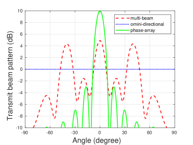
Figure 1: Three different types of transmit beam patterns for radar: omni-directional, multi-beam and phased-array single beam.

VI-B Balanced SINR versus transmit SNR

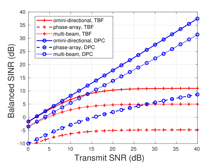
Figure 2: Balanced SINR versus transmit SNR $P/\sigma^{2}$, for $K=4$. ”TBF” is the curve for transmit beamforming.

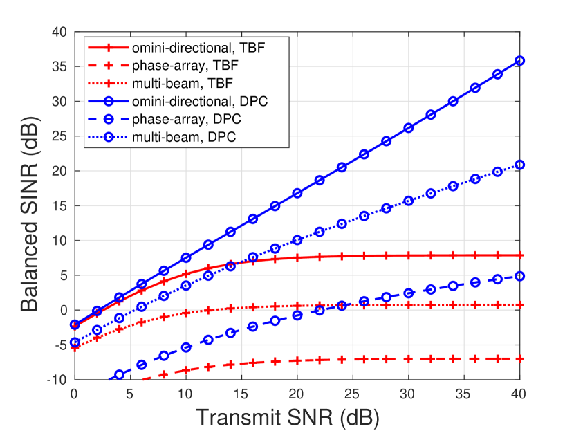
Figure 3: Balanced SINR versus transmit SNR $P/\sigma^{2}$, for $K=6$. ”TBF” is the curve for transmit beamforming.

The balanced SINR under different transmit SNR and $\bm{S}_{o}$ for $K=4$ is displayed in Fig. 3, in both transmit beamforming and DPC regimes. From Fig. 3, it is observed that DPC achieves higher balanced SINR than transmit beamforming. The performance improvement of DPC over transmit beamforming is especially impressive under a high transmit SNR. For omni-directional and multi-beam patterns, the balanced SINR via DPC increases linearly with the transmit SNR in dB scale, while the counterpart for transmit beamforming does not increase when the transmit SNR is high. The reason is that the interference cannot be effectively canceled via transmit beamforming with the transmit covariance constraint. To zero-forcing the interference, transmit beamforming requires $\bm{S}_{h}=\bm{H}\bm{S}_{o}\bm{H}^{H}$ to be a diagonal matrix [16], while this condition generally does not hold if $\bm{H}$ is Rayleigh fading. Since the interference cannot be eliminated, the balanced SINR for transmit beamforming keeps constant even if the SNR is high. Conversely, DPC are still able to cancel the interference under the transmit covariance constraint. As explained in Sec. II-D, to zero-forcing the interference in the DPC regime, we only need $\bm{S}_{h}$ to be non-singular. This condition can be met if the rank of $\bm{S}_{o}$, denoted by $r_{o}$, is not less than $K$ when $\bm{H}$ obeys Rayleigh fading. We note that the value of $r_{o}$ are $10$, $4$ and $1$ for the omni-directional, multi-beam and phased-array pattern, respectively. When $K=4$, the condition holds for omni-directional and multi-beam patterns, and thus the corresponding balanced SINR for DPC is respectable under a high SNR. For phased-array mode, $r_{o}$ is less than $K$, and thus its balanced SINR in the DPC regime becomes much lower compared to omni-directional and multi-beam patterns. Nevertheless, DPC is still able to achieve an acceptable balanced SINR for phased-array beam when the transmit SNR is high, while we observe that the counterpart via transmit beamforming is even less than $0$-dB.

The balanced SINR versus transmit SNR for $K=6$ is shown in Fig. 3. By comparing Fig. 3 and Fig. 3, one observes that the balanced SINR becomes lower when $K$ increases, namely the service quality for each user can worsen when the number of users increases. We also observe that the loss of balanced SINR in the DPC regime is slight for omni-directional beam pattern, but is notable for the multi-beam pattern. We note that when $K=6$, $r_{o}$ is larger than $K$ for omni-directional beam pattern, and thus DPC is still able to zero-forcing the interference. However, for the multi-beam pattern, $r_{o}$ is less than $K=6$, and thus ZF DPC is not applicable, leading to an obvious performance degradation. Based on the above facts, we can regard the $r_{o}$, the rank of $\bm{S}_{o}$, as the degrees of freedom of the communication transmitter. In the DPC regime, increasing $K$ generally does not cause serious loss of service quality if $K$ does not exceed the degrees of freedom, while the loss can be more significant when $K$ exceeds it. It is worth noting that when $K$ exceeds $r_{o}$, simultaneously servicing for $K$ users via transmit beamforming is almost unrealistic, since the balanced SINR is extremely low.

VI-C Maximized sum rate versus transmit SNR

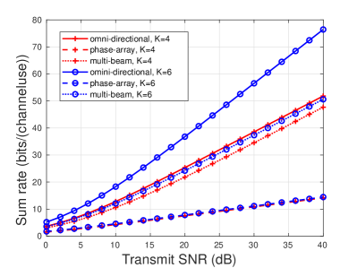
Figure 4: Maximized sum rate versus transmit SNR $P/\sigma^{2}$, for $K=4,6$.

The maximized sum rate versus transmit SINR in the DPC regime is given in Fig. 4, for $K=4,6$. In Fig. 4, the sum rate is asymptotically affine in the transmit SNR in dB, and the slope of the line determines the multiplexing gain [39, 36] of multiuser communications, which equals to the rate gain in bits/channeluse for every $3$-dB transmit power gain. With a power constraint, it is proven in [36] that the multiplexing gain of the GBC is $K$. With the considered transmit covariance constraint, the results is different. For instance, we read from Fig. 4 that the multiplexing gain for the multi-beam pattern does not increase when $K$ increases from $4$ to $6$. A similar result is observed from the curve for phase-array mode. Nevertheless, for omni-directional beam pattern, the multiplexing gain increases from $4$ to $6$ when $K$ increases from $4$ to $6$. In summary, one can find that the multiplexing gain is $\min\{K,r_{o}\}$ with the transmit covariance constraint. The explanation is from the fact that ZF DPC is asymptotic optimal under a high SNR. When $K\leq r_{o}$, the GBC can be simplified to $K$ AWGN channels to the $K$ users via ZF DPC, and thus the multiplexing gain is $K$. However, when $K>r_{o}$, to meet the constraint $\bm{F}\bm{F}^{H}\preceq\bm{R}_{h}$, $\bm{F}$ should have at most $r_{o}$ non-zero diagonal elements if it is lower triangular. In other words, to zero forcing the interference, only $r_{o}$ users are active while the others are inactive. Therefore, when $K>r_{o}$, the multiplexing gain is restricted by $r_{o}$, and the sum rate gain is not obvious if $K$ exceeds $r_{o}$.

VI-D Convergence performance of the iteration algorithms

The convergence performance of the iteration algorithms to solve the SINR balancing problem for transmit beamforming in Sec. III-B is displayed in Fig. 6. In Fig. 6, the SINR gap $\gamma^{(\ell)}-\gamma^{*}$ versus iteration time $\ell$ in $10$ experiments with randomly distributed $\bm{H}$ is demonstrated, for $K=4$, $\bm{S}_{o}=(1/M)\bm{I}_{M}$ and $P=10$. Here, $\gamma^{*}$ is the balanced SINR obtained by the linear conic programming in (17), and $\gamma^{(\ell)}$ is the temporary SINR after the $\ell$-th iteration, given by

$$t^{(\ell)}:=\mathrm{{tr}}\Big{\{}(\bm{D}^{(\ell)}\bm{[}D^{(\ell)}]^{H})^{1/2}\Big{\}},\ \gamma^{(\ell)}:=[t^{(\ell)}]^{2}/(1-[t^{(\ell)}]^{2}).$$

From Fig. 6, we observe that the iteration algorithm in Sec. III-B converges fast. In some experiments, the SINR gap is less than $10^{-4}$ after no more than $10$ iterations. We note that the optimal $\bm{d}$ in (20) may locate at the boundary, i.e. have zero elements. In this case, the algorithm may need more iterations to converge, as indicated by the curves in the right of Fig. 6. Nevertheless, the algorithm can still find an acceptable approximate solution with a few iterations. Considering the interference control, the number of users for transmit beamforming should be limited. Therefore, the dimension of the variable $\bm{d}$ can be low in practice, and it is hopeful to implement the algorithm in real time.

The convergence performance of the iterative algorithms to solve the SINR balancing problem for DPC in Sec. IV-B is displayed in Fig. 6, which gives the SINR gap $\gamma^{(\ell)}-\gamma_{o}^{*}$ versus iteration time $\ell$ in $10$ experiments. In each experiment, $\bm{H}$ is randomly generated with $K=4$, and $\bm{S}_{o}=(1/M)\bm{I}_{M}$. To perform the experiments, we first let the balanced SINR be $\gamma_{o}^{*}=10$, next compute the minimal power $P^{\prime}$ to achieve the SINR by solving (27), and then perform the iteration algorithm to solve (28) with the power $P^{\prime}$, i.e. with $\bm{R}_{o}=P^{\prime}\bm{S}_{o}$.

Compared with the the iteration algorithm for transmit beamforming, the algorithm for DPC needs more iterations to achieve a small SINR gap. This is mainly because the optimization in (28) has a more complex structure and a higher dimension than that in (20). In the experiments, we observe that the iterations converge within a moderate number of times when the optimal $\bm{Y}$ is non-singular, while the SINR gap decreases slower when the optimal $\bm{Y}$ is singular. For practical applications, a trade-off between the accuracy and computation time can be considered. In other words, we can control the number of iterations and obtain an approximate solution. To improve the algorithm efficiency, one may further consider deep leaning enabled acceleration schemes as in [27].

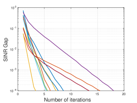
Figure 5: The SINR gap $\gamma^{(\ell)}-\gamma^{*}$ versus iteration time $\ell$ for the SINR balancing in the transmit beamforming regime.

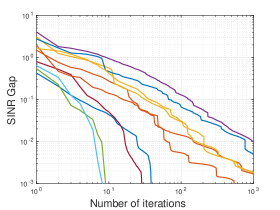
Figure 6: The SINR gap $\gamma^{(\ell)}-\gamma_{o}^{*}$ versus iteration time $\ell$ for the SINR balancing in the DPC regime.

VII Conclusion

In this paper, we consider the transmit design of a joint MIMO radar and downlink multiuser communications system, in which the communication performance is optimized under a transmit covariance constraint from radar. In particular, we formulate the SINR balancing problem in both transmit beamforming and DPC regimes, and the sum rate maximization in the DPC regime. Further, we proposed methods to solve these problems via convex optimization. Despite the low complexity of transmit beamforming, the achievable SINR via transmit beamforming may be low even if the transmit SNR is high. As the theoretically optimal scheme for multiuser precoding, DPC has a impressive performance gain over transmit beamforming, with increased complexity for encoding and optimization. In the simulations, it is observed that the degrees of freedom for the communication transmitter is restricted by the rank of the transmit covariance.

Appendix A The Lagrange dual of (18)

The dual objective function is defined by $g_{1}(\bm{Y},\bm{d})=\max_{\bm{F}_{u},t}\mathcal{L}_{1}(\bm{F}_{u},t,\bm{Y},\bm{d})$. Under the conditions that

$$\bm{s}^{T}\bm{d}=1,\ d_{k}\bm{u}_{k}\in\mathcal{C}(\bm{Y})\ \mathrm{for}\ k=1,\ldots,K,$$ (55)

where $\bm{s}=[s_{1},\ldots,s_{K}]^{T}$, $g_{1}(\bm{Y},\bm{d})$ is finite and its expression is

$$g_{1}(\bm{Y},\bm{d})=\mathrm{tr}\Big{\{}\bm{Y}+\frac{1}{4}\bm{Y}^{\dagger}\bm{D}\bm{D}^{H}\Big{\}},$$ (56)

where $\bm{D}=\left[d_{1}\bm{u}_{1},\ldots,d_{K}\bm{u}_{K}\right]$. Thus, the Lagrange dual problem of (18) is

$$\min_{\bm{Y},\bm{d}}\mathrm{tr}\Big{\{}\bm{Y}+\frac{1}{4}\bm{Y}^{\dagger}\bm{D}\bm{D}^{H}\Big{\}},\ \mathrm{s.t.}\ \eqref{eq-dual-condition1},\ \bm{d}\geq 0,\ \bm{Y}\succeq 0.$$ (57)

To solve the dual problem, we consider to optimize $\bm{Y}$ with a given $\bm{d}$. From equation (2.4) in [50], one has

$$\mathrm{tr}\Big{\{}\bm{Y}+\frac{1}{4}\bm{Y}^{\dagger}\bm{D}\bm{D}^{H}\Big{\}}\geq\mathrm{tr}\Big{\{}(\bm{Y}\bm{Y}^{\dagger}\bm{D}\bm{D}^{H})^{1/2}\Big{\}}=\mathrm{tr}\Big{\{}(\bm{D}\bm{D}^{H})^{1/2}\Big{\}},$$ (58)

where the inequality holds with equality when $\bm{Y}=\frac{1}{2}(\bm{D}\bm{D}^{H})^{1/2}$. In (58), we use the equality that $\bm{Y}\bm{Y}^{\dagger}\bm{D}=\bm{D}$ since the columns of $\bm{D}$ should be in $\mathcal{C}(\bm{Y})$ according to (55). Note that (58) gives the optimal value of (57) under a given $\bm{d}$. Therefore, the dual problem in (57) is equivalent to (20).

Appendix B Computation of the projection onto $\Omega_{1}$

The projection of a point $\bm{d}=[d_{1},\ldots,d_{K}]^{T}\in\mathbb{R}^{K}$ onto $\Omega_{1}$ is expressed as

$$\bm{x}=\arg\min_{\hat{\bm{x}}}\frac{1}{2}\|\bm{d}-\hat{\bm{x}}\|_{2}^{2},\ \mathrm{s.t.}\ \hat{\bm{x}}\geq 0,\ \bm{s}^{T}\hat{\bm{x}}=1,$$ (59)

where $\bm{s}=[s_{1},\ldots,s_{K}]^{T}>0$. Letting $\bm{\theta}=[\theta_{1},\ldots,\theta_{K}]^{T}\geq 0$ and $v$ be the dual variables associated with the constrains $\hat{\bm{x}}\geq 0$ and $\bm{s}^{T}\hat{\bm{x}}=1$, ${\bm{x}}$ should be the solution of the KKT system [29]:

$$x_{k}=d_{k}+\theta_{k}-vs_{k}=0,\bm{s}^{T}\bm{x}=1,\theta_{k}x_{k}=0,x_{k}\geq 0,\theta_{k}\geq 0,$$ (60)

where $x_{k}$ is the $k$-th element in $\bm{x}$, for $k=1,\ldots,K$.

To solve (60), we let $r_{k}=d_{k}/s_{k}$. Without loss of generality, it is assumed that $r_{1}\leq\cdots\leq r_{K}$. First, we note that $v$ should obey $v<r_{K}$. If $v\geq r_{K}$, we have $x_{k}^{2}=x_{k}\theta_{k}+x_{k}(d_{k}-vs_{k})\leq 0$ for all $k$. Then $\bm{x}=0$, which is not feasible. There should exist an integer $1\leq j\leq K$ such that $v\in[r_{j-1},r_{j})$. If $j=1$, the interval is $(-\infty,r_{1})$. Similarly, we have $x_{k}=0$ for all $k<j$. In addition, for $k\geq j$, we have $x_{k}-\theta_{k}=d_{k}-vs_{k}>0$, so $\theta_{k}=0$. Based on these conclusions, we have

$$x_{k}=0,\ \forall k<j,\ x_{k}=d_{k}-vs_{k},\ \forall k\geq j.$$ (61)

Since $\bm{s}^{T}\bm{x}=1$, $v$ should be given by

$$v=\frac{\sum_{k=j}^{K}d_{k}-1}{\sum_{k=j}^{K}s_{k}}.$$ (62)

The problem is that $j$ is unknown. Nevertheless, we can search for a $j$ so that $v(j)\in[r_{j-1},r_{j})$, where $v(j)$ is the value of $v$ computed by (62). Since $j$ is an integer in $[1,K]$, the times of searching is not larger than $K$. Once $j$ is obtained, the projection $\bm{x}$ can be computed via (61) and (62).

Appendix C The dual of (25)

The Lagrange function [29] of (27) is

$$\mathcal{L}_{2}(\bm{F}_{u},\lambda,\bm{Y},\bm{d})=\lambda+\mathrm{tr}\big{(}\bm{Y}(\bm{F}_{u}\bm{F}_{u}^{H}-\lambda\bm{I}_{r})\big{)}+\sum_{k=1}^{K}d_{k}\Big{\{}\sum_{i>k}\left|\bm{u}_{k}^{H}\bm{f}_{i}\right|^{2}+1-\frac{1}{\gamma}\left|\bm{u}_{k}^{H}\bm{f}_{k}\right|^{2}\Big{\}},$$ (63)

where $\bm{d}=\left[d_{1},\ldots,d_{K}\right]^{T}\geq 0$ and $\bm{Y}\succeq 0$ are dual variables. The dual function is $g_{2}(\bm{Y},\bm{d})=\min_{\bm{F}_{u},\lambda}\mathcal{L}_{2}(\bm{F}_{u},\lambda,\bm{Y},\bm{d})$. It can be shown that $g_{2}(\bm{Y},\bm{d})$ is finite under the conditions of (28b) and (28c) [38], repeated as follows:

$$\mathrm{tr}(\bm{Y}) =1,$$ (28b)

$$\bm{Y}+\sum_{i<k}d_{i}\bm{u}_{i}\bm{u}_{i}^{H} \succeq\frac{1}{\gamma}d_{k}\bm{u}_{k}\bm{u}_{k}^{H},\ k=1,\ldots,K.$$ (28c)

When these conditions hold, the dual function is given by $g_{2}(\bm{Y},\bm{d})=\sum_{k=1}^{K}d_{k}$. Therefore, the dual problem of (27) is

$$\max_{\bm{Y}\succeq 0}\ \max_{\bm{d}\geq 0}\ \sum_{k=1}^{K}d_{k},\ \ \mathrm{s.t.}\ \eqref{eq-dual-cond-a}\ \mathrm{and}\ \eqref{eq-dual-cond-b}.$$ (65)

It can be proven that (27) has strong duality [38], so the optimal value of (65), denoted by $\lambda_{\mathrm{dual}}^{*}(\gamma)$, equals to $\lambda^{*}(\gamma)$. Then, $\gamma_{o}^{*}$ should satisfy $\lambda_{\mathrm{dual}}^{*}(\gamma_{o}^{*})=1$. In other words, $\gamma_{o}^{*}$ is the minimal $\gamma\geq 0$ so that $\lambda_{\mathrm{dual}}^{*}(\gamma)\geq 1$. Note that $\lambda_{\mathrm{dual}}^{*}(\gamma)\geq 1$ means there exists a pair of feasible solution $\bm{Y},\bm{d}$ in (65) satisfying $\sum_{k=1}^{K}d_{k}\geq 1$. Therefore, $\gamma_{o}^{*}$ is equal to the optimal value of the dual problem in (28).

Appendix D The gradient of the objective function in (31)

To derive the gradient, we note that $\gamma_{o}(\bm{Y}),\bm{d}^{*}(\bm{Y})$ is the solution of the equations in (30). When $\bm{Y}\succ 0$, the index set $\mathcal{I}(\bm{Y})$ is empty. Computing the differential to the equations in (30), we have

$$\bm{1}_{K}^{T}\mathrm{d}\bm{d}=0,$$ (66a)

$$\mathrm{d}\gamma-\mathrm{d}d_{k}\bm{u}_{k}^{H}\bm{f}_{k}^{*}(\bm{Y})=-d_{k}^{*}(\bm{Y})[\bm{f}_{k}^{*}(\bm{Y})]^{H}(\mathrm{d}\bm{Y}+\sum_{i<k}\mathrm{d}d_{i}\bm{u}_{k}\bm{u}_{k}^{H})\bm{f}_{k}^{*}(\bm{Y}),$$ (66b)

for $k=1,\ldots,K$. We rewrite (66b) into a matrix form:

$$\bm{A}\mathrm{d}\bm{d}=\mathrm{d}\gamma\bm{1}_{K}+\bm{b},$$ (67)

where the $k$-th element in $\bm{b}$ is $d_{k}^{*}(\bm{Y})[\bm{f}_{k}^{*}(\bm{Y})]^{H}\mathrm{d}\bm{Y}\bm{f}_{k}^{*}(\bm{Y})$ and $\bm{A}$ is defined in (33). Combining (66a) and (67), one has

$$\bm{1}_{K}^{T}\bm{A}^{-1}\bm{1}_{K}\mathrm{d}\gamma+\bm{1}_{K}^{T}\bm{A}^{-1}\bm{b}=0.$$ (68)

Letting $a_{k}$ be the $k$-th element in $\bm{a}=(\bm{A}^{-1})^{T}\bm{1}_{K}$, there is

$$\mathrm{d}\gamma=-\frac{1}{\sum_{k=1}^{K}a_{k}}\mathrm{tr}\Big{\{}\sum_{k=1}^{K}a_{k}d_{k}^{*}(\bm{Y})\hat{\bm{f}}_{k}^{*}(\bm{Y})[\hat{\bm{f}}_{k}^{*}(\bm{Y})]^{H}\mathrm{d}\bm{Y}\Big{\}},$$ (69)

from which one can obtain the gradient in (34).

Appendix E Computation of the projection onto $\Omega_{2}$

The projection of a Hermitian matrix $\bm{Y}\in\mathbb{C}^{r\times r}$ onto $\Omega_{2}$ is

$$\arg\min_{{\bm{X}}}\frac{1}{2}\|\bm{Y}-{\bm{X}}\|_{F}^{2},\ \mathrm{s.t.}\ \mathrm{tr}({\bm{X}})=1,\ {\bm{X}}\succeq 0.$$ (70)

To solve (70), we write the eigen decomposition of $\bm{Y}$ as $\bm{Y}=\bm{V}\bm{\Sigma}_{y}\bm{Y}^{H}$, where $\bm{V}$ is a $r\times r$ unitary matrix and $\bm{\Sigma}_{y}$ is diagonal. Letting $\bm{\Sigma}_{x}=\bm{V}^{H}{\bm{X}}\bm{V}$, the optimization in (70) is reformulated to

$$\min_{\bm{\Sigma}_{x}}\frac{1}{2}\|\bm{\Sigma}_{y}-\bm{\Sigma}_{x}\|_{F}^{2},\ \mathrm{s.t.}\ \mathrm{tr}({\bm{\Sigma}}_{x})=1,\ {\bm{\Sigma}}_{x}\succeq 0.$$ (71)

It can be observed that $\bm{\Sigma}_{x}$ should be diagonal at the optimum. We let $y_{k}$ and $x_{k}$ be the $(k,k)$-th elements in $\bm{\Sigma}_{y}$ and $\bm{\Sigma}_{x}$, respectively. Then (71) is equivalent to

$$\min_{\bm{x}}\frac{1}{2}\|\bm{y}-\bm{x}\|_{2}^{2},\ \mathrm{s.t.}\ \bm{1}_{r}^{T}\bm{x}=1,\ \bm{x}\geq 0.$$ (72)

where $\bm{x}=[x_{1},\ldots,x_{r}]^{T}$ and $\bm{y}=[y_{1},\ldots,y_{r}]^{T}$. Here, (72) has the same form as the optimization in (59), and can be solved with no more than $K$ loops. Once the optimal $\bm{x}$ is obtained, the projection is given by $\bm{V}\mathrm{diag}(\bm{x})\bm{V}^{H}$.

Appendix F Proof for Theorem 1

In this proof, we verify that $\bm{Y}^{*}$ and $\bm{d}^{*}$ meet the KKT condition of (45), which is stated as

$$({\bm{Y}}^{*}+\sum_{k=1}^{K}d_{k}^{*}\bm{u}_{k}\bm{u}_{k}^{H})^{-1}-[\bm{Y}]^{*-1}+\nu\bm{I}_{r}=\bm{0},$$ (73a)

$$\mathrm{tr}({\bm{Y}^{*}})=1,\ {\bm{Y}}^{*}\succ 0,$$ (73b)

$$\bm{u}_{j}^{H}({\bm{Y}}^{*}+\sum_{k=1}^{K}d_{k}^{*}\bm{u}_{k}\bm{u}_{k}^{H})^{-1}\bm{u}_{j}-\eta+\varphi_{j}=0,$$ (73c)

$$\sum_{k=1}^{K}d_{k}^{*}=1,\ d^{*}_{j}\geq 0,\ \varphi_{j}\geq 0,\ \varphi_{j}d_{j}^{*}=0,$$ (73d)

for $j=1,\ldots,K$. Here, $\nu$, $\eta$ and $\{\varphi_{k}\}$ are the dual variables associated with the constraints $\mathrm{tr}(\bm{Y})=1$, $\sum_{k=1}^{K}d_{k}=1$ and $\bm{d}\geq 0$, respectively, and their values are given by

$$\eta=\bm{1}_{K}^{T}\bm{\phi},\ \nu=\eta,\ \varphi_{k}=\eta\Big{(}1-\bm{u}_{k}^{H}{\bm{Z}}^{*}\bm{u}_{k}\Big{)},$$ (74)

for $k=1,\ldots,K$.

In the following, we check the conditions in (73) one by one. First, we point out an important relationship between $\bm{d}^{*}$, ${\bm{Y}}^{*}$ and ${\bm{Z}}^{*}$. From (52), one has

$$(1/\eta)[{\bm{Z}}^{*}]^{-1}=\bm{Y}^{*}+\sum_{k=1}^{K}d_{k}^{*}\bm{u}_{k}\bm{u}_{k}^{H}.$$ (75)

Then

$$({\bm{Y}}^{*}+\sum_{k=1}^{K}d_{k}^{*}\bm{u}_{k}\bm{u}_{k}^{H})^{-1}-[\bm{Y}^{*}]^{-1}=\eta{\bm{Z}}^{*}-[\bm{Y}^{*}]^{-1}=-\nu\bm{I}_{r},$$

i.e. (73a) holds, and

$$\bm{u}_{j}^{H}({\bm{Y}}^{*}+\sum_{ki=1}^{K}d_{k}^{*}\bm{u}_{k}\bm{u}_{k}^{H})^{-1}\bm{u}_{j}=\eta\bm{u}_{j}^{H}\bm{Z}^{*}\bm{u}_{j}=\eta-\varphi_{k},$$

i.e. (73c) holds. In (73b), ${\bm{Y}}^{*}\succ 0$ is trivial, and

$$\mathrm{tr}({\bm{Y}}^{*})=\frac{1}{\eta}\mathrm{tr}((\bm{Z}^{*}+\bm{I}_{r})^{-1})=\frac{r}{\eta}-\frac{1}{\eta}\mathrm{tr}((\bm{Z}^{*}+\bm{I}_{r})^{-1}\bm{Z}^{*}).$$ (76)

Multiply the left and right side of (52) by ${\bm{Z}}^{*}$ and take the matrix trace, we have

$$\mathrm{tr}((\bm{Z}^{*}+\bm{I}_{r})^{-1}\bm{Z}^{*})=r-\sum_{k=1}^{K}\phi_{k}\bm{u}_{k}^{H}\bm{Z}^{*}\bm{u}_{k}.$$ (77)

Substituting (77) into (76), one has

$$\mathrm{tr}(\bm{Y}^{*})=\frac{1}{\eta}\sum_{k=1}^{K}\phi_{k}\bm{u}_{k}^{H}\bm{Z}^{*}\bm{u}_{k}=\frac{1}{\eta}\sum_{k=1}^{K}\phi_{k}=1,$$ (78)

so (73b) holds. Finally we show that (73d) holds. The first three conditions in (73d) are trivial. According to (52), it can be shown that

$$\varphi_{j}d_{j}^{*}=\phi_{j}(1-\bm{u}_{j}^{H}{\bm{Z}}^{*}\bm{u}_{j})=0.$$ (79)

Therefore (73d) holds and the proof is completed.

References

- [1] B. Paul, A. R. Chiriyath, and D. W. Bliss, “Survey of RF communications and sensing convergence research,” IEEE Access, vol. 5, pp. 252–270, 2017.
- [2] F. Liu, C. Masouros, A. Li, H. Sun, and L. Hanzo, “MU-MIMO communications with MIMO radar: From co-existence to joint transmission,” IEEE Transactions on Wireless Communications, vol. 17, no. 4, pp. 2755–2770, Apr. 2018.
- [3] D. Ma, N. Shlezinger, T. Huang, Y. Liu, and Y. C. Eldar, “Joint radar-communication strategies for autonomous vehicles: Combining two key automotive technologies,” IEEE Signal Processing Magazine, vol. 37, no. 4, pp. 85–97, 2020.
- [4] C. Sturm and W. Wiesbeck, “Waveform design and signal processing aspects for fusion of wireless communications and radar sensing,” Proceedings of the IEEE, vol. 99, no. 7, pp. 1236–1259, 2011.
- [5] Y. Zhang, Q. Li, L. Huang, C. Pan, and J. Song, “A modified waveform design for radar-communication integration based on LFM-CPM,” in 2017 IEEE 85th Vehicular Technology Conference (VTC Spring), Jun. 2017, pp. 1–5.
- [6] P. M. McCormick, S. D. Blunt, and J. G. Metcalf, “Simultaneous radar and communications emissions from a common aperture, part I: Theory,” in 2017 IEEE Radar Conference (RadarConf), May 2017, pp. 1685–1690.
- [7] P. Kumari, J. Choi, N. González-Prelcic, and R. W. Heath, “IEEE 802.11ad-based radar: An approach to joint vehicular communication-radar system,” IEEE Transactions on Vehicular Technology, vol. 67, no. 4, pp. 3012–3027, Apr. 2018.
- [8] F. Liu, L. Zhou, C. Masouros, A. Li, W. Luo, and A. Petropulu, “Toward dual-functional radar-communication systems: Optimal waveform design,” IEEE Transactions on Signal Processing, vol. 66, no. 16, pp. 4264–4279, Aug. 2018.
- [9] M. F. Keskin, V. Koivunen, and H. Wymeersch, “Limited feedforward waveform design for OFDM dual-functional radar-communications,” IEEE Transactions on Signal Processing, vol. 69, pp. 2955–2970, 2021.
- [10] S. D. Blunt, M. R. Cook, and J. Stiles, “Embedding information into radar emissions via waveform implementation,” in 2010 International Waveform Diversity and Design Conference, Aug. 2010, pp. 000 195–000 199.
- [11] A. Hassanien, M. G. Amin, Y. D. Zhang, and F. Ahmad, “Dual-function radar-communications: Information embedding using sidelobe control and waveform diversity,” IEEE Transactions on Signal Processing, vol. 64, no. 8, pp. 2168–2181, Apr. 2016.
- [12] A. Hassanien, M. G. Amin, Y. D. Zhang, and F. Ahmad, “Phase-modulation based dual-function radar-communications,” IET Radar, Sonar Navigation, vol. 10, no. 8, pp. 1411–1421, 2016.
- [13] X. Wang, A. Hassanien, and M. G. Amin, “Dual-function MIMO radar communications system design via sparse array optimization,” IEEE Transactions on Aerospace and Electronic Systems, pp. 1–1, 2018.
- [14] T. Huang, N. Shlezinger, X. Xu, Y. Liu, and Y. C. Eldar, “MAJoRCom: A dual-function radar communication system using index modulation,” IEEE Transactions on Signal Processing, vol. 68, pp. 3423–3438, 2020.
- [15] D. Ma, N. Shlezinger, T. Huang, Y. Shavit, M. Namer, Y. Liu, and Y. C. Eldar, “Spatial modulation for joint radar-communications systems: Design, analysis, and hardware prototype,” IEEE Transactions on Vehicular Technology, vol. 70, no. 3, pp. 2283–2298, 2021.
- [16] X. Liu, T. Huang, N. Shlezinger, Y. Liu, J. Zhou, and Y. C. Eldar, “Joint transmit beamforming for multiuser MIMO communications and MIMO radar,” IEEE Transactions on Signal Processing, vol. 68, pp. 3929–3944, 2020.
- [17] F. Liu, Y.-F. Liu, A. Li, C. Masouros, and Y. C. Eldar, “Cramér-rao bound optimization for joint radar-communication design,” 2021.
- [18] P. Stoica, J. Li, and Y. Xie, “On probing signal design for MIMO radar,” IEEE Transactions on Signal Processing, vol. 55, no. 8, pp. 4151–4161, Aug. 2007.
- [19] D. R. Fuhrmann and G. S. Antonio, “Transmit beamforming for MIMO radar systems using signal cross-correlation,” IEEE Transactions on Aerospace and Electronic Systems, vol. 44, no. 1, pp. 171–186, Jan. 2008.
- [20] J. Li, L. Xu, P. Stoica, K. W. Forsythe, and D. W. Bliss, “Range compression and waveform optimization for MIMO radar: A Cramer-Rao bound based study,” IEEE Transactions on Signal Processing, vol. 56, no. 1, pp. 218–232, Jan. 2008.
- [21] I. Bekkerman and J. Tabrikian, “Target detection and localization using MIMO radars and sonars,” IEEE Transactions on Signal Processing, vol. 54, no. 10, pp. 3873–3883, 2006.
- [22] F. Rashid-Farrokhi, K. R. Liu, and L. Tassiulas, “Transmit beamforming and power control for cellular wireless systems,” IEEE Journal on Selected Areas in Communications, vol. 16, no. 8, pp. 1437–1450, 1998.
- [23] E. Visotsky and U. Madhow, “Optimum beamforming using transmit antenna arrays,” in 1999 IEEE 49th Vehicular Technology Conference (Cat. No.99CH36363), vol. 1, May 1999, pp. 851–856 vol.1.
- [24] A. Wiesel, Y. C. Eldar, and S. Shamai, “Zero-forcing precoding and generalized inverses,” IEEE Transactions on Signal Processing, vol. 56, no. 9, pp. 4409–4418, Sep. 2008.
- [25] E. Björnson, M. Bengtsson, and B. Ottersten, “Optimal multiuser transmit beamforming: A difficult problem with a simple solution structure [lecture notes],” IEEE Signal Processing Magazine, vol. 31, no. 4, pp. 142–148, Jul. 2014.
- [26] A. Wiesel, Y. C. Eldar, and S. Shamai, “Linear precoding via conic optimization for fixed MIMO receivers,” IEEE Transactions on Signal Processing, vol. 54, no. 1, pp. 161–176, Jan. 2006.
- [27] J. Zhang, W. Xia, M. You, G. Zheng, S. Lambotharan, and K.-K. Wong, “Deep learning enabled optimization of downlink beamforming under per-antenna power constraints: Algorithms and experimental demonstration,” IEEE Transactions on Wireless Communications, vol. 19, no. 6, pp. 3738–3752, 2020.
- [28] D. G. Luenberger and Y. Ye, Conic Linear Programming. Cham: Springer International Publishing, 2016, pp. 149–176.
- [29] S. Boyd and L. Vandenberghe, Convex Optimization. Cambridge University Press, 2004.
- [30] M. Costa, “Writing on dirty paper (Corresp.),” IEEE Transactions on Information Theory, vol. 29, no. 3, pp. 439–441, May 1983.
- [31] G. Caire and S. Shamai, “On the achievable throughput of a multiantenna Gaussian broadcast channel,” IEEE Transactions on Information Theory, vol. 49, no. 7, pp. 1691–1706, 2003.
- [32] P. Viswanath and D. N. C. Tse, “Sum capacity of the vector Gaussian broadcast channel and uplink–downlink duality,” IEEE Transactions on Information Theory, vol. 49, no. 8, pp. 1912–1921, Aug. 2003.
- [33] S. Vishwanath, N. Jindal, and A. Goldsmith, “Duality, achievable rates, and sum-rate capacity of Gaussian MIMO broadcast channels,” IEEE Transactions on Information Theory, vol. 49, no. 10, pp. 2658–2668, Oct. 2003.
- [34] Wei Yu and J. M. Cioffi, “Sum capacity of Gaussian vector broadcast channels,” IEEE Transactions on Information Theory, vol. 50, no. 9, pp. 1875–1892, 2004.
- [35] H. Weingarten, Y. Steinberg, and S. S. Shamai, “The capacity region of the Gaussian multiple-input multiple-output broadcast channel,” IEEE Transactions on Information Theory, vol. 52, no. 9, pp. 3936–3964, Sep. 2006.
- [36] J. Lee and N. Jindal, “Dirty paper coding vs. linear precoding for MIMO broadcast channels,” in 2006 Fortieth Asilomar Conference on Signals, Systems and Computers, Oct. 2006, pp. 779–783.
- [37] M. Sharif and B. Hassibi, “A comparison of time-sharing, DPC, and beamforming for MIMO broadcast channels with many users,” IEEE Transactions on Communications, vol. 55, no. 1, pp. 11–15, 2007.
- [38] W. Yu and T. Lan, “Transmitter optimization for the multi-antenna downlink with per-antenna power constraints,” IEEE Transactions on Signal Processing, vol. 55, no. 6, pp. 2646–2660, 2007.
- [39] L. Zheng and D. Tse, “Communication on the Grassmann manifold: a geometric approach to the noncoherent multiple-antenna channel,” IEEE Transactions on Information Theory, vol. 48, no. 2, pp. 359–383, 2002.
- [40] K. Petersen and M. Pedersen, The Matrix Cookbook. Technical University of Denmark, 2006, version 20051003.
- [41] T. Cover, “Broadcast channels,” IEEE Transactions on Information Theory, vol. 18, no. 1, pp. 2–14, 1972.
- [42] J. Gallier, “The Schur complement and symmetric positive semidefinite (and definite) matrices,” [EB/OL], https://www.cis.upenn.edu/~jean/schur-comp.pdf, August 24, 2019.
- [43] E. J. Candes and T. Tao, “The power of convex relaxation: Near-optimal matrix completion,” IEEE Transactions on Information Theory, vol. 56, no. 5, pp. 2053–2080, 2010.
- [44] M. Grant and S. Boyd, “CVX: Matlab software for disciplined convex programming, version 2.1,” http://cvxr.com/cvx, Mar. 2014.
- [45] ——, “Graph implementations for nonsmooth convex programs,” in Recent Advances in Learning and Control, ser. Lecture Notes in Control and Information Sciences, V. Blondel, S. Boyd, and H. Kimura, Eds. Springer-Verlag Limited, 2008, pp. 95–110, http://stanford.edu/~boyd/graph_dcp.html.
- [46] E. G. Birgin, J. M. Martínez, and M. Raydan, “Nonmonotone spectral projected gradient methods on convex sets,” SIAM Journal on Optimization, vol. 10, no. 4, pp. 1196–1211, 2000.
- [47] A. Mokhtari, A. Ozdaglar, and S. Pattathil, “A unified analysis of extra-gradient and optimistic gradient methods for saddle point problems: Proximal point approach,” in Proceedings of the Twenty Third International Conference on Artificial Intelligence and Statistics, ser. Proceedings of Machine Learning Research, S. Chiappa and R. Calandra, Eds., vol. 108. PMLR, 26–28 Aug 2020, pp. 1497–1507. [Online]. Available: https://proceedings.mlr.press/v108/mokhtari20a.html
- [48] A. Juditsky and A. Nemirovski, “On well-structured convex–concave saddle point problems and variational inequalities with monotone operators,” Optimization Methods and Software, vol. 0, no. 0, pp. 1–36, 2021.
- [49] K.-K. K. Kim, “Optimization and Convexity of ),” International Journal of Control, Automation and Systems, vol. 17, no. 4, pp. 1067–1070, Apr. 2019. [Online]. Available: https://doi.org/10.1007/s12555-018-0263-y
- [50] K. Shebrawi and H. Albadawi, “Trace inequalities for matrices,” Bulletin of the Australian Mathematical Society, vol. 87, no. 1, p. 139–148, 2013.