Double-, triple-line spectroscopic candidates in the LAMOST Medium-Resolution Spectroscopic Survey

Abstract

The LAMOST Medium-Resolution Spectroscopic Survey (LAMOST-MRS) provides an unprecedented opportunity for detecting multi-line spectroscopic systems. Based on the method of Cross-Correlation Function (CCF) and successive derivatives, we search for spectroscopic binaries and triples and derive their radial velocities (RVs) from the LAMOST-MRS spectra. A Monte-Carlo simulation is adopted to estimate the RV uncertainties. After examining over 1.3 million LAMOST DR7 MRS blue arm spectra, we obtain 3,133 spectroscopic binary (SB) and 132 spectroscopic triple (ST) candidates, which account for 1.2% of the LAMOST-MRS stars. Over 95% of the candidates are newly discovered. It is found that all of the ST candidates are on the main sequence, while around 10% of the SB candidates may have one or two components on the red giant branch.

1 Introduction

Since approximately half of the stars in our Galaxy are in double, triple or high-order systems (Raghavan et al., 2010), multiple star systems play an essential role in astrophysics, especially binary systems. The characterization of multiple star systems such as orbital parameters can be investigated by combining the spectroscopic and photometric information.

Spectroscopic multiple star systems can be classified according to the number of stellar components in the spectra, because their spectral lines split due to the different radial velocities (RVs). A target can be considered as a spectroscopic binary (SB) or spectroscopic triple (ST) candidate if it has a double- or triple-line spectrum. The single-line SBs can also be identified as their radial velocities are variable.

Up to now, some catalogs of the spectroscopic multiple star systems have been published, $\rm S_{B^{9}}$, the recent version of the ninth catalogue of spectroscopic binary orbits includes more than 4,004 SBs, and around one third of them are double-line systems (Pourbaix et al., 2004), and the Geneva-Copenhagen Survey Catalogue presents 3,223 SBs from 16,682 nearby F and G dwarf stars (Nordström et al., 2004; Holmberg et al., 2009). The recent spectroscopic surveys provide a bulk of spectra, which have largely expanded the number of spectroscopic multiple star systems, such as the Radial Velocity Experiment (RAVE) survey (Matijevič et al., 2010) has found 123 SBs, the Gaia-ESO survey (Merle et al., 2017) has detected 342 SB, 11 ST and even 1 quadruple-line candidates, the Apache Point Observatory Galaxy Evolution Experiment (APOGEE) survey has discovered more than 3,000 binaries (Fernandez et al., 2017; El-Badry et al., 2018), and the Galactic Archaeology with HERMES (GALAH) survey has derived 12,760 FGK SBs with stellar properties (Traven et al., 2020).

The Large Sky Area Multi-Object fiber Spectroscopic Telescope (LAMOST) is a 4-meter Schmidt telescope with a 5° field of view (FOV), and is equipped with 4,000 fibers (Cui et al., 2012; Luo et al., 2015; Zhao et al., 2006, 2012). The medium-resolution spectroscopic (MRS) survey includes both blue and red arms, and the wavelength coverages of them are from 4,950 to 5,350 Å  and from 6,300 to 6,800 Å, respectively. The resolution power of MRS is 7,500. There are more absorption lines in the blue arm than those in the red one, which enables us to measure the RVs with a precision of 1 km/s for most of the stars (Liu et al., 2019). The efficiency of observations and the achieved precisions make LAMOST-MRS an exceptional database for measuring RVs and detecting multiple star systems.

The purpose of this work is to detect the multiple-line candidates (SB and ST) from the LAMOST-MRS database following the method of Merle et al. (2017). This paper is organized as follows, in Sect. 2, we describe the LAMOST-MRS spectral dataset. The methods used to normalize spectra, calculate CCFs and detect peak positions in CCFs are introduced in Sect. 3, and a catalog that contains SB and ST candidates detected from LAMOST-MRS is presented in Sect. 4. In Sect. 5, we discuss the detection efficiency, the stellar parameters of the SB and ST candidates, radial velocity differences and caveats, and the conclusions are given in Sect 6.

2 Data Selection

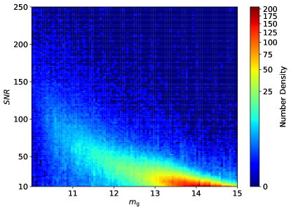
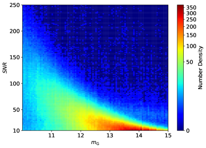
Figure 1: The distributions of SNR versus SDSS g magnitude of the first year survey (upper panel) and the Gaia DR2 G magnitude of the second year survey (lower panel).

The LAMOST-MRS test observation started in Sep. 2017, and the LAMOST-MRS survey began in Oct. 2018. The first and second year MRS data has been released in the LAMOST Data Release 7 (DR7). The wavelength ranges of the LAMOST-MRS blue and red arms are from 4,950 to 5,350 Å and from 6,300 to 6,800 Å. Until April 11, 2019, the LAMOST-MRS survey has obtained 5,369,891 spectra of 759,886 objects. Only the spectra of blue arms have been chosen to detect multiple line candidates and measure their RVs, as there are more absorption lines in the blue arms. The distributions of the signal-to-noise ratio (SNR) of the blue arm spectra versus the SDSS g magnitude of the first year survey and the Gaia DR2 G magnitude of the second year survey are displayed in Figure 1. It can be seen that most of the objects have g or G magnitudes between 10 and 15. It is found that a spectrum with low SNR will lead to challenges for detecting reliable SBs and STs (Fernandez et al., 2017). Therefore, the blue arm spectra with SNR higher than 10 have been selected. In addition to SNR, the header keywords objtype and fibermas have also been taken into consideration. Only these spectra with objtype of star and fibermas of 0 have been chosen, because the header keyword fibermas of not 0 indicates that this fiber may have problems. Finally, 1,383,831 spectra of 281,437 stars have been selected.

Figure 2 shows the number of exposures for these stars, and most of them have been observed three times because the LAMOST-MRS no-time-domain observation takes three consecutive exposures (Liu et al., 2020). The number and Cumulative Distribution Function (CDF) versus SNR of all the selected spectra are presented in Figure 3.

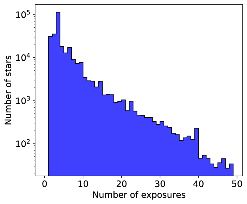
Figure 2: Number of selected stars versus number of exposures. The number of stars is in $log$ scale.

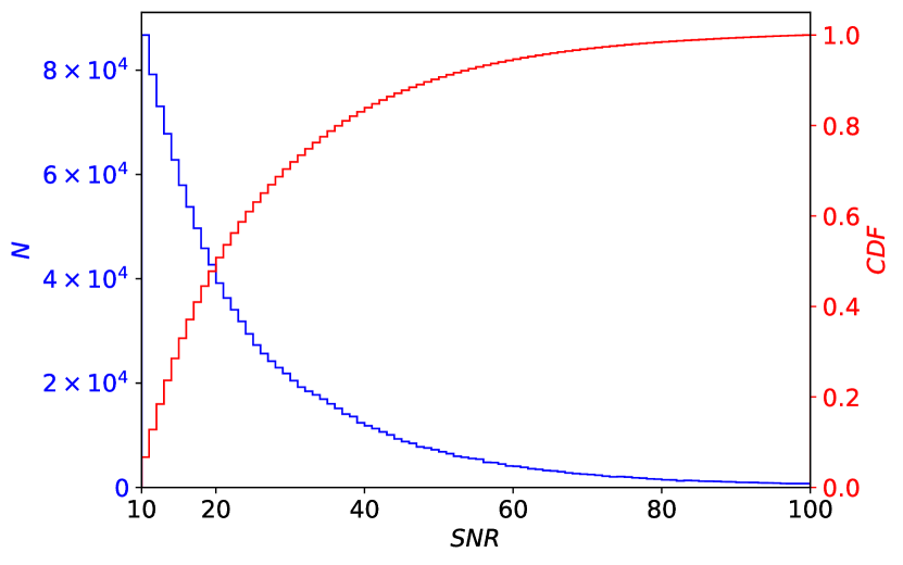
Figure 3: Number and Cumulative Distribution Function (CDF) diagram of SNR of all the selected spectra.

3 Method

Based on the Gaia-ESO survey, Merle et al. (2017) have developed a method to search for multi-line spectroscopic candidates. Their method utilizes the Gaussian kernel to smooth the successive derivatives of Cross-Correlation Function (CCF). Following their method, we detect SB and ST candidates and derive their RVs from the LAMOST-MRS spectra. A Monte-Carlo (MC) simulation is adopted to estimate the RV uncertainties for each spectrum.

3.1 Calculating CCF

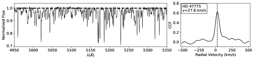
Figure 4: The normalized LAMOST-MRS spectra (left panel) and CCF diagrams (right panel) of HD 47775.

CCF is usually used to measure RVs and to find multiple line spectra. We use Eq. 1 to calculate the values of the normalized CCF according to the normalized correlation coefficient (Gubner, 2006, p. 92). The range of the normalized CCFs is between $-$1 and $+$1, with $+$1 indicating a perfect correlation and $-$1 for a perfect anti-correlation.

$$CCF(v)=\displaystyle\sum_{i=1}^{n}\frac{(O_{i}-\overline{O})}{\sigma_{O}}\cdot\frac{(T_{i,v}-\overline{T})}{\sigma_{T}},$$ (1)

Here, $O_{i}$ and $T_{i,v}$ are the normalized flux of the observed and template spectra at a same wavelength sampling point $i$, and the RV value of the template is located at v. $\overline{O}$ and $\sigma_{O}$ are the mean and scatter of the flux values of the observed spectrum, while $\overline{T}$ and $\sigma_{T}$ for the template. In this work, we generate a set of template spectra with a series of RVs based on the normalized solar spectrum (Kurucz et al., 1984). The RV variations are from $-$500 to $+$500 km/s with a step of 1 km/s. To decrease the sampling points, we reduce the resolution of the templates to 100,000.

It is noted that the peaks in some CCFs are too low to be detected, therefore, these spectra with a maximum value of CCF less than 0.2 and/or the difference between the maximum and minimum values of CCF less than 0.1, have been not considered. About 80,000 spectra have been excluded by these criteria.

The spectra need to be normalized, and we apply a general normalization procedure to all the selected spectra. The normalization procedure is as follows:

1. Splitting each spectrum evenly into 10 bins by wavelength,

2. Quadratic spline interpolation with the median flux values of the 10 bins,

3. Masking the cosmic-rays, absorption and emission lines.

As the cosmic-rays and emission lines will lead to negative values of CCF, they need to be masked during normalization. Thus, we calculate the standard deviation ($\sigma$) of the residual between the observed spectrum and the continuum, and mask these points where the residuals are higher than $+5\sigma$.

The whole process is iterated three times to improve the continuum. The left panel of Figure 4 shows an example, the normalized spectrum of HD 47775.

3.2 Detecting the number of RV components and determining their RVs

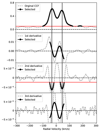
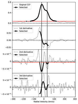
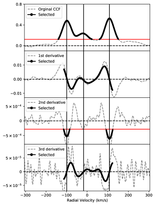
Figure 5: CCFs and derivatives of two SB and one ST candidates. The gray dashed lines are the original CCFs and derivatives, all the selected range of CCFs and smoothed derivatives are drawn with black solid lines. The red horizontal lines are the thresholds for each candidate, and the black vertical lines are their RVs.

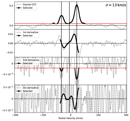
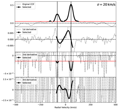
Figure 6: The example of finding an appropriate $\sigma$ of Gaussian smoothing.

To obtain the number of RV components and their values, Merle et al. (2017) have designed a detection of extrema code to identify the peaks in CCFs. In their Figure 1, Merle et al. (2017) presented simulated CCFs and their derivatives, there is a peak in the CCF diagram, where is the value of RV. By detecting where the 1st derivative passes zero in declining phase or the 3rd derivative passes zero in ascending phase, it is possible to identify the RV components of the spectrum and calculate their RV values.

We note that small bulges (CCF values are around zero) can also be identified as peaks for the 1st or 3rd derivatives, for instance, in the right panel of Figure 5. The reason is that there are more noises in the higher-order derivatives for a discrete CCF. To avoid the impact of these spurious peaks, it is necessary to select the RV range and smooth the derivatives. Therefore, the Gaussian filter function gaussian_filter1d of the scipy.ndimage package (Virtanen et al., 2020) in Python is adopted to smooth the derivatives.

Two thresholds are used to select the RV range, the first one is the percentile of the CCF, and the other one is the percentile of the smoothed 2nd derivative. Only the ranges where the CCF values are higher than the 75th percentile and the smoothed 2nd derivative values are lower than the 6th percentile have been selected, as shown in Figure 5. If the selected ranges are separate, some triple-line spectra would be identified as double-line (see the right panel of Figure 5). Thus, the middle part between the separate ranges are also selected.

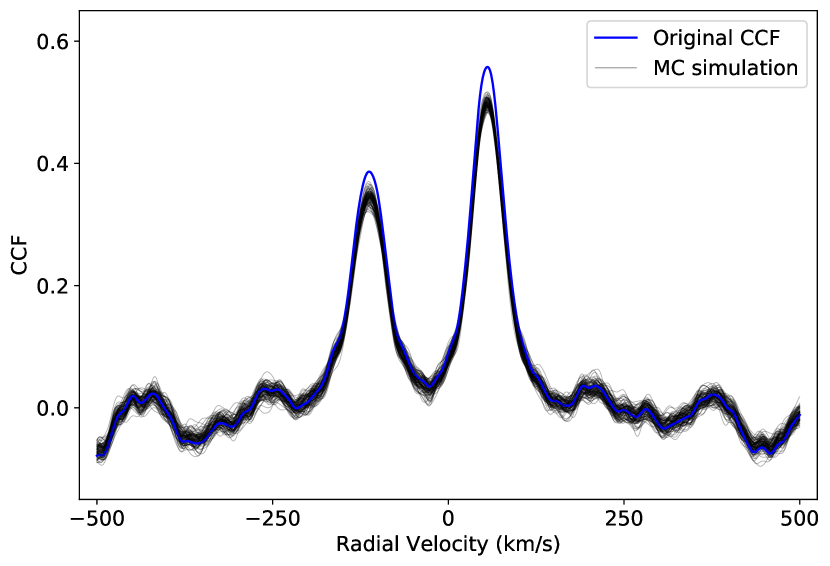
Figure 7: Original CCF of a double-line spectrum and MC simulation ones.

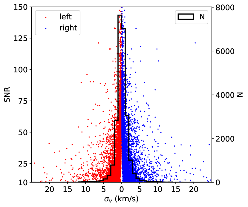
Figure 8: The SNR of spectra verses the RV uncertainties of SB candidates. Red and blue dots are the radial velocity of the left and right peak of CCF.

As shown in the middle panel of Figure 5, the two peaks are strongly blended in the CCF diagram, and only one peak can be detected by the 1st derivative. While, there are still two peaks can be detected from the 3rd derivative, therefore, we derive the RVs from the 3rd derivatives. A linear fit using the two near zero points of the ascending 3rd derivative is adopted to calculate the RV value.

An appropriate standard deviation ($\sigma$) of the Gaussian kernel is important for smoothing, and we choose an initial $\sigma$=13 km/s for the LAMOST-MRS spectra. However, this value is too small for some cases, and it may lead to extra spurious RV component as shown in the left panel of Figure 6. In this case, we increase the $\sigma$ by 1 km/s till the number of RV components detected with the 3rd derivative is equal to the number of valleys in the 2nd derivative, and the $\sigma$ has been increased from 13 km/s to 20 km/s (see the right panel of Figure 6).

3.3 Uncertainties

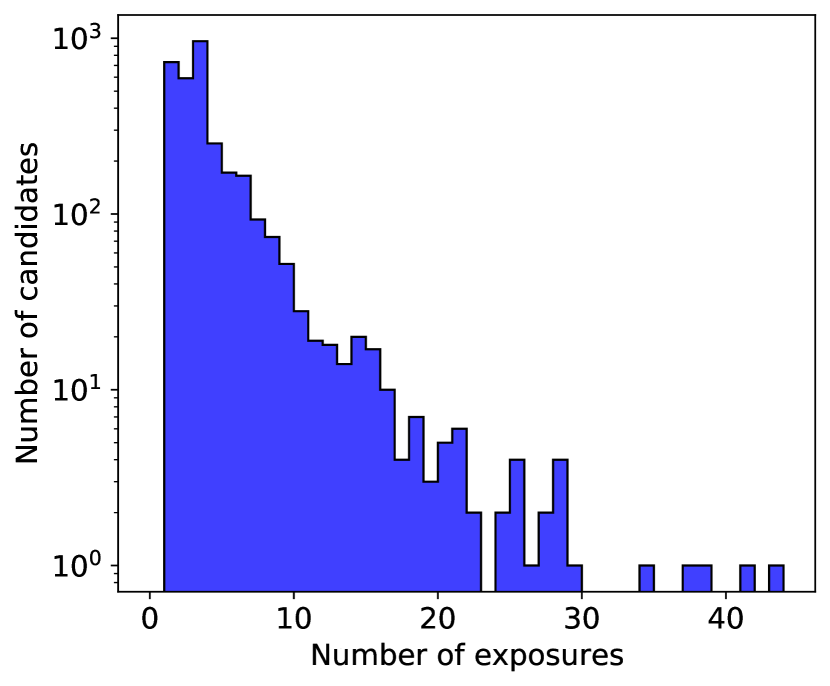
Figure 9: Number of the detected SB and ST candidates versus number of exposures. The number of stars is in $log$ scale.

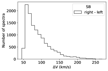
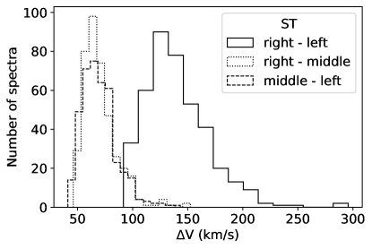
Figure 10: The number distribution of SB and ST spectra RV difference.

A Monte-Carlo (MC) simulation is applied to estimate the uncertainties of our RV measurements. The main idea is to generate a set of simulated spectra based on each observed spectrum, and derive their RV values from the CCFs. For each RV component, we take the standard deviation of these RVs as its RV uncertainty.

For each observed spectrum, we generate 100 simulated spectra. For a simulated spectrum, the flux at each wavelength point is a random value generated from a Gaussian distribution, and the mean and variance of the Gaussian distribution are the flux and flux error of the corresponding observed spectrum. The CCFs of an observed spectrum and the 100 simulated spectra are presented in Figure 7. We notice that the amplitudes of the simulated CCFs are lower than that of the observed one, because the process of generating simulated spectra introduces additional error, therefore, the SNRs of the simulated spectra are lower than that of the observed spectrum.

It should be noted that if the number of RV components detected from the simulated spectrum is different from the observed one, this spectrum is discarded.

Figure 8 shows the distribution of SNR and RV uncertainties of all the detected SB candidates. The scatter of the RV errors ($\sim$ 1 km/s) is in line with the value of Liu et al. (2019) for LAMOST-MRS spectra.

4 Results

After examining the LAMOST-MRS spectra, we detect 3,133 SB and 132 ST candidates, which account for 1.2% of the LAMOST-MRS stars.

4.1 SB and ST candidates and RVs

There are 14,647 double- and 1,065 triple-line spectra having been detected with this method, and 11,648 double- and 388 triple-line spectra are confirmed after checking the CCF diagrams by human eyes. The proportions are 80% and 36% for the double- and triple-line spectra, respectively.

We present all the SB and ST candidates and their RV values and uncertainties in Table 1, including the celestial coordinates, source id from Gaia Early Data Release 3 (Gaia Collaboration et al., 2020), Gaia G magnitude and the number of exposures. Four spectral information from the LAMOST data release: the LAMOST MRS plan name (planID), spectrograph ID (spID), fiber ID and Local Modified Julian Minute (LMJM), is also presented. It need to be pointed out that the RV values rv1, rv2 and rv3 are arranged in order of values, as it is difficult to identify which RV component corresponds to each star when they have similar spectral type.

We consider a star to be ST candidate as long as one of its spectra has been detected three RV components. Accordingly, we classified 41 stars with both double- and triple-line spectra as ST candidates. The RV variations indicate that they are probably physical binaries or triples. Further checking the RV variations of these candidates will help us to identify more physical multiple star systems.

Figure 9 shows the distribution of the number of exposures of the detected candidates. There are 525 SB and 31 ST candidates with more than 6 observations, they are needed to be investigated as their orbital parameters may be derived by RV curves.

The detected RV difference limit is around 50 km/s for all of the SB and ST candidates (Figure 10), which meets the resolution of the LAMOST-MRS spectra. The largest RV differences are around 250 km/s and 300 km/s for SB and ST candidates, respectively.

In order to improve the detection efficiency, a human-free method is needed. Among the machine learning and deep learning techniques, the Recurrent Neural Network (RNN) is proved to be highly-performant for this classification (Jamal & Bloom, 2020). To test the feasibility, we designed a RNN to derive the peak numbers from the CCF diagrams. Our RNN is trained by the CCF diagrams of the confirmed SB and ST candidates, and the details about the RNN can be found in Appendix A. The total classification accuracy of our RNN is 0.96, which is a significant improvement compared to the traditional method. Therefore, we will use RNN to detect SB and ST candidates in future study.

4.2 New binary candidates

We cross-match our LAMOST-MRS SB and ST candidates with these of the other binary catalogues, including $\rm S_{B^{9}}$ (Pourbaix et al., 2004), the Geneva-Copenhagen Survey of Solar neighbourhood III (Holmberg et al., 2009), the RAVE SB2 (Matijevič et al., 2010), the Gaia-ESO multi-line SB (Merle et al., 2017), the Washington Visual Double Star (WDS, Mason et al., 2001), the binaries of APOGEE (Fernandez et al., 2017; El-Badry et al., 2018), the FGK binary stars of the GALAH survey (Traven et al., 2020) and the third revision of Kepler Eclipsing Binary Catalog (KEBIII, Kirk et al., 2016), and there are 107 stars in common. The information about these stars are listed in Table B1.

Except for these common stars, there are 3,034 SB and 124 ST candidates (over 95% of the total candidates) newly discovered. These RVs can be used to derive the orbital parameters of these systems (Pan et al., 2021; Wang et al., 2021).

=0.5in

Table 1: The information of SB, ST candidates and their RVs.

RA(2000)	DEC(2000)	Gaia source id	G(mag)	SB/ST	$N_{\rm Exp}$	planID	spID	fiberID	LMJM	SNR	rv1 (km/s)	rv2 (km/s)	rv3 (km/s)
0.01948	57.48923	422589945455866496	12.1	SB	1	HIP11784201	9	62	83604881	17	$-36.7\pm 0.7$	$20.7\pm 0.7$	-
0.13490	63.87285	431630508024107392	12.7	SB	1	NGC778801	12	27	83650762	15	$-57.0\pm 3.3$	$39.5\pm 15.1$	-
0.23830	40.43928	2881984048448075264	12.4	SB	1	HIP11776901	6	17	83609143	14	$-58.5\pm 0.8$	$-6.9\pm 0.5$	-
0.29125	58.69553	422768646150973696	12.2	SB	3	NGC778901	12	240	83647859	15	$-9.3\pm 5.5$	$62.6\pm 1.6$	-
0.29125	58.69553	422768646150973696	12.2	SB	3	NGC778901	12	240	83647873	14	$-11.0\pm 5.6$	$63.7\pm 7.8$	-
0.29125	58.69553	422768646150973696	12.2	SB	3	NGC778901	12	240	83647886	16	$-19.2\pm 7.5$	$59.8\pm 8.5$	-
0.34767	41.11409	2882225867991453056	12.2	SB	9	HIP11776901	6	39	83604805	21	$-95.4\pm 0.4$	$32.4\pm 0.7$	-
0.34767	41.11409	2882225867991453056	12.2	SB	9	HIP11776901	6	39	83604818	20	$-96.0\pm 0.3$	$31.0\pm 0.8$	-
0.34767	41.11409	2882225867991453056	12.2	SB	9	HIP11776901	6	39	83604832	22	$-94.6\pm 0.3$	$30.9\pm 0.7$	-
0.34767	41.11409	2882225867991453056	12.2	SB	9	HIP11776901	6	39	83607704	27	$-85.3\pm 0.6$	$9.2\pm 0.4$	-
$\cdots$	$\cdots$	$\cdots$	$\cdots$	$\cdots$	$\cdots$	$\cdots$	$\cdots$	$\cdots$	$\cdots$	$\cdots$	$\cdots$	$\cdots$	$\cdots$
5.34918	58.28837	422132853553794816	12.9	ST	3	NT002740N583314C02	3	187	84196452	49	$-72.7\pm 1.5$	$-0.4\pm 1.5$	$61.1\pm 2.2$
5.34918	58.28837	422132853553794816	12.9	ST	3	NT002740N583314C02	3	187	84196476	47	$-69.6\pm 1.9$	$-2.2\pm 1.0$	$58.6\pm 2.0$
5.34918	58.28837	422132853553794816	12.9	ST	3	NT002740N583314C02	3	187	84196499	49	$-74.7\pm 1.4$	$-1.4\pm 1.1$	$63.1\pm 2.4$
17.51845	2.00869	2538630790708445312	10.7	ST	4	TD010605N031628K01	7	113	84118991	58	$-20.9\pm 0.5$	$63.4\pm 0.4$	-
17.51845	2.00869	2538630790708445312	10.7	ST	4	TD010605N031628K01	7	113	84119014	50	$-20.3\pm 0.6$	$64.6\pm 0.5$	-
17.51845	2.00869	2538630790708445312	10.7	ST	4	TD010605N031628K01	7	113	84119038	39	$-18.5\pm 0.6$	$65.7\pm 0.7$	-
17.51845	2.00869	2538630790708445312	10.7	ST	4	TD010605N031628K01	7	113	84166383	46	$-65.7\pm 0.5$	$-15.6\pm 0.4$	$79.5\pm 0.5$
18.16407	45.78222	400867753213471744	11.9	ST	4	TD012220N453143T01	14	68	84156353	15	$-97.8\pm 2.1$	$0.2\pm 3.1$	-
18.16407	45.78222	400867753213471744	11.9	ST	4	TD012220N453143T01	14	68	84156377	14	$-97.3\pm 2.3$	$-0.5\pm 3.6$	-
18.16407	45.78222	400867753213471744	11.9	ST	4	TD012220N453143T01	14	68	84156400	12	$-95.3\pm 1.6$	$3.2\pm 1.5$	-
18.16407	45.78222	400867753213471744	11.9	ST	4	TD012220N453143T01	14	68	84156423	11	$-96.3\pm 2.2$	$-46.4\pm 3.5$	$0.3\pm 2.2$
$\cdots$	$\cdots$	$\cdots$	$\cdots$	$\cdots$	$\cdots$	$\cdots$	$\cdots$	$\cdots$	$\cdots$	$\cdots$	$\cdots$	$\cdots$	$\cdots$

Note. — The RV values rv1, rv2 and rv3 are arranged in order of values. 41 ST candidates show both double- and triple-line spectra.

5 Discussion

5.1 Detection efficiency

To test the detection efficiency of the method, we use the radiative transfer code SPECTRUM (Gray & Corbally, 1994) and the Kurucz (Kurucz, 1979) stellar atmosphere models to generate six synthetic spectra of given stellar parameters. They include cool and hot ($T_{\rm eff}=5000,8000$ K), giant and dwarf ($\log{g}$ = 2.0, 4.0 dex), metal-rich and metal-poor ([Fe/H] = 0.0, $-$2.0 dex) models. All of the synthetic spectra have been reduced to the same wavelength range and resolution (R$\sim$7,500) as the LAMOST-MRS blue arm ones. We generate a set of double-line synthetic spectra by shifting a synthetic spectrum with different RVs and combining it with the original ones, and the synthetic double-line SBs have equal masses.

A similar MC simulation (see in Sect 3.3) is adopted to test the detection efficiency. We add the random Gaussian distribution noises to each point of the synthetic spectrum and generate 100 spectra for a specific SNR to detect RV components. We count the number of spectra detected as SBs, and the success rate represents the detection efficiency.

Our simulation results are presented in Figure 11, and it can be seen that the detection limit of RV differences is between 40 and 50 km/s, and this limit is consistent with the LAMOST-MRS resolution power. The detection efficiency of the method is similar except for hot metal-poor dwarfs.

5.2 Stellar parameters

It is useful to investigate the distribution of stellar atmospheric parameters of SB and ST candidates, although the general method for determining the stellar atmospheric parameters may not be appropriate for multi-line spectra. We adopt the stellar atmospheric parameters of 1,470 SB and 65 ST candidates from the LAMOST DR7 low-resolution spectroscopic survey (LAMOST-LRS) (Luo et al., 2015), and present their distribution in $T_{\rm eff}$ vs $\log{g}$, $T_{\rm eff}$ vs [Fe/H], and $\log{g}$ vs [Fe/H] in Figure 12.

We note that about 90% of the SB and all the ST candidates are on the main sequence, only 155 SBs may have one or two components on the red giant branch ($\log{g}<3.5$ dex). The reason is that when the massive component climbs the red giant branch, its radius increases, and mass transfer occurs after it reaches the Roche lobe. The interaction between the components can modify the evolution and lead to fewer giant binary systems. The lack of metal-poor candidates is due to less low metallicity stars in our sample.

5.3 Caveats

There are some caveats we need to be pointed out before utilizing the SB or ST catalog for further studies. Since the completeness of the multi-line spectroscopic candidate catalog is not the primary goal of this work, the selection effects of the LAMOST-MRS data and the detecting process of the method must be considered in the further statistical studies.

Another caveat is that the SB and ST candidates are not necessarily physical binaries or triples. The CCFs of double- and triple-line spectra may be mimicked by emission lines or stellar pulsations, etc. (Merle et al., 2017). Considering the LAMOST fibers have a diameter of 3.3 arcsec (Cui et al., 2012), one spectrum may contain light from multiple stars when they are very close to each other in the sky. Investigating the RV variations of the SB and ST candidates is essential to identify the physical binaries and triples.

6 Conclusions

Based on the method of CCF and Gaussian smooth for the derivatives of CCF, we detected 14,647 double- and 1,065 triple-line spectra from the blue arm spectra with SNR$\geqslant$10 of the LAMOST DR7 MRS. After checking the CCF diagrams by human eyes, 11,648 double-line and 388 triple-line spectra are confirmed, the proportions are 80% and 36%, respectively. They belong to 3,133 SB and 132 ST candidates, these confirmed candidates account for 1.2% of the LAMOST-MRS stars. Among the ST candidates, 41 of them show double- and triple-line cases, which indicates that they are physical binaries because of the variations of RVs. Comparing with the other binary star catalogs, we find that about 95 percent of them are newly discovered. For the 1,470 SB and 65 ST candidates, which have stellar atmospheric parameters from the LAMOST-LRS survey, 90% of the SB and all the ST candidates are on the main sequence.

A Monte-Carlo simulation is used to estimate the RV uncertainties, and the RV error is of the order of 1 km/s. Our results indicate that the detection limit of RV differences is between 40 and 50 km/s.

The LAMOST-MRS survey is going on, and will provide a great opportunity of studying the binary and multiple star systems.

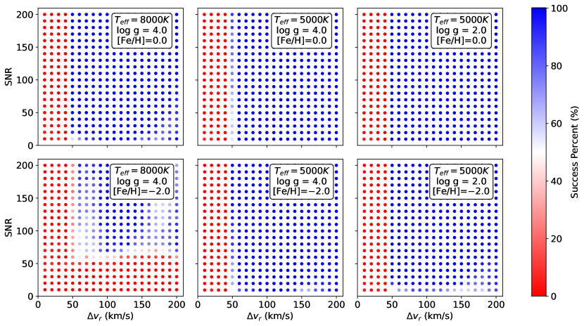
Figure 11: The detection efficiency of simulated SB in different atmospheric parameters, RV differences and SNR levels.

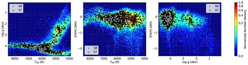
Figure 12: The distribution of stellar atmospheric parameters of common stars between the LAMOST DR7 Low-Resolution Spectroscopic Survey and the selected LAMOST-MRS data. The black cross are the SB candidates, and white pentagons are ST candidates. The left panel is $T_{\rm eff}$ vs $\log{g}$ diagram, the middle panel is $T_{\rm eff}$ vs [Fe/H] diagram, and the right panel is $\log{g}$ vs [Fe/H] diagram. All the atmospheric parameters are provided by the LAMOST DR7 LRS.

Acknowledgments We thank the referee for the helpful comments which have helped us to improve the manuscript. Our research is supported by National Key R&D Program of China No.2019YFA0405502, the National Natural Science Foundation of China under grant Nos. 12090040, 12090042, 12090044, 11833002, 11833006, 12022304, 11973052, 11973042 and U1931102. This work is supported by the Astronomical Big Data Joint Research Center, co-founded by the National Astronomical Observatories, Chinese Academy of Sciences and Alibaba Cloud. H.-L.Y. acknowledges the supports from Youth Innovation Promotion Association, Chinese Academy of Sciences (id. 2019060) and NAOC Nebula Talents Program. Guoshoujing Telescope (the Large Sky Area Multi-Object Fiber Spectroscopic Telescope LAMOST) is a National Major Scientific Project built by the Chinese Academy of Sciences. Funding for the project has been provided by the National Development and Reform Commission. LAMOST is operated and managed by the National Astronomical Observatories, Chinese Academy of Sciences.

Appendix A Detecting Peaks

We design a simple Recurrent Neural Network (RNN) to inspect the peak numbers of CCF diagrams automatically. Because of the incremental data of the LAMOST-MRS survey, a human-free classification method is urgently need to analyze these spectra. Among mostly-used machine learning and deep learning (DL) techniques, RNN proves to be highly-performant for the classification of 1-dimension data (Jamal & Bloom, 2020) compared to the Convolutional Neural Network (CNN).

Recurrent neural network (RNN) refers to a class of artificial neural networks where network architecture composed of interconnected nodes through a directed graph along a temporal sequence. The Long-Short Term Memory (LSTM, Hochreiter & Schmidhuber, 1997) is one of the variants of RNN with gated state or memory. The LSTM has been found extremely successful in many applications, such as speech recognition (Graves et al., 2013), handwriting generation (Graves, 2013), and machine translation (Sutskever et al., 2014). At the same time, RNNs have been applied on astronomical data (Jamal & Bloom, 2020) including variable stars (Naul et al., 2018), periodic variable stars (Tsang & Schultz, 2019) and supernovae classifications, (Charnock & Moss, 2017) and online transient event detection (Muthukrishna et al., 2019; Möller & de Boissière, 2020).

We set up our RNN with a 3-layer LSTM, the hidden size of 256 units, and 3 output features. This RNN is trained by 12,136 CCF diagrams with labels as number of peaks (0, 2, 3) together with 4,046 groups of test data. We split the training data into batches to speed up the training process. After 100 training epochs, we stop the training process to avoid the overfitting (with a training loss of 0.003 and test loss of 0.100). The final classification accuracy and precision are shown in Table A1 and the confusion matrix obtained on the Test set predictions for the RNN classifier is shown in Figure A1.

Table A1: The precision, recall and f1-score of the prediction of classification.

Peak number	Precision	Recall	F1-score
0	0.91	0.92	0.92
2	0.97	0.97	0.97
3	0.84	0.72	0.78

F1-score is the harmonic mean of precision and recall:

$$F_{1}=\frac{2}{{\rm precision}^{-1}+{\rm recall}^{-1}}$$ (A1)

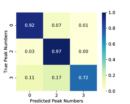
Figure A1: Confusion matrix obtained on the Test set predictions for the RNN classifier. The values in each box refer to the number of predictions versus the true labels.

The recognization of two peaks is performed well (precision $\sim 0.97$) since there are the most training data of two peaks CCFs. On the contrary, the group of three peaks is the most difficult one for recognization due to less data. Totally, the final classification accuracy is 0.96, which means that, for a given CCF diagram, we can detect the correct peak number successfully by the probability of 0.96. This method can improve the productiveness and robustness. We use the deep learning method along with human eyes to confirm our results.

Appendix B Common SB and ST candidates with other binary catalogs

Table B1: List of the common SB and ST candidates with other binary catalogs.

RA(2000)	DEC(2000)	Gaia source id	G	SB/ST	$N_{\rm Exp}$	Catalog
4.31148	0.55870	2545576336943059072	12.7	SB	3	GALAH
6.35503	59.11604	428267308105062528	11.1	SB	4	WDS
9.78481	59.81764	425556805786609408	10.9	SB	14	WDS
10.17108	57.76887	424898679355325312	11.3	SB	2	WDS
13.49841	10.08698	2582339740871439360	12.2	SB	1	GALAH
15.04087	12.21674	2584289591599704064	11.5	SB	1	GALAH
15.23534	11.58956	2584040273042478208	12.8	SB	2	GALAH
19.44386	0.62884	2535048989846592768	13.1	SB	2	GALAH
29.76969	58.39781	505491850882835584	11.0	ST	3	WDS
31.96472	13.79138	77202449462513024	12.1	SB	3	APOGEE
46.84714	40.80111	239854583246385408	10.3	SB	1	WDS
46.91366	66.17673	492339320985355648	10.6	SB	3	WDS
50.59945	51.66556	442912798683449088	12.1	ST	9	WDS
51.47665	18.13560	55926869402261760	12.5	SB	4	GALAH
51.85738	19.01199	57544044849005440	13.0	SB	2	GALAH
52.37579	19.41492	57640320835799808	12.3	SB	4	GALAH
55.16722	45.77760	244833962172857728	11.2	ST	3	WDS
62.05420	19.94418	51832421242688128	12.4	SB	3	WDS
63.01352	48.26905	246251095218220160	11.0	SB	1	WDS
63.01540	21.94700	52684199156684032	8.9	SB	3	SB9, WDS
63.29504	61.55950	475258132965412224	13.1	SB	3	WDS
66.44780	18.31499	3314466360138302592	13.0	SB	2	GALAH
68.20363	16.02178	3312652582565893632	13.0	SB	9	GALAH
71.04484	26.76769	154533339923810688	13.7	SB	11	GALAH
71.43970	23.53370	146573528573114240	12.9	SB	4	GALAH
71.99216	22.95037	3413141584496385792	12.0	SB	11	GALAH
72.16204	15.36070	3405024886580964736	12.9	SB	3	GALAH
72.21994	14.71636	3308722103373770496	13.4	SB	3	GALAH
72.40034	56.28887	274601899464974592	10.6	SB	3	WDS
73.58480	20.85980	3411716548707061376	11.7	ST	8	GALAH
73.72125	24.23559	3419659356282987008	12.5	SB	9	GALAH
74.90812	21.79690	3412251701632573312	11.7	ST	5	GALAH
75.05998	24.13008	3419410763576132352	10.9	ST	12	WDS
76.05618	24.30754	3418774008905352704	10.3	SB	3	WDS
77.57841	24.48785	3419012499849582464	11.5	SB	3	GALAH
83.88432	35.85607	183166645640035584	11.9	SB	3	WDS
92.23265	22.14776	3423547328182688640	10.9	SB	1	WDS
98.13701	8.59674	3326258557925415936	11.2	SB	3	WDS
98.72293	9.43785	3326828345466157952	10.8	SB	5	WDS
100.44896	9.86729	3326737665818107008	13.1	SB	2	Gaia ESO
101.89452	8.47141	3134190163070718464	10.4	ST	7	WDS
101.93376	23.12819	3379557723381624832	11.2	SB	3	WDS
102.21957	17.33513	3358396660030939776	12.0	SB	6	WDS
103.79022	22.80749	3380050961721719680	10.5	SB	7	WDS
106.83926	45.75925	977374646347674624	12.5	SB	3	WDS
115.99661	24.74451	867894834757702400	13.5	SB	1	WDS
123.65855	14.73966	655293644368357120	11.7	SB	3	GALAH
123.72821	16.71239	655829140890694016	13.0	SB	5	GALAH
123.85360	16.22931	655726439632891648	12.7	SB	3	GALAH
124.00038	17.45520	657004106505230336	12.6	SB	4	GALAH
124.14557	19.41296	663514555370788224	12.4	SB	7	GALAH
124.24190	17.65389	657014483146180352	11.8	SB	4	GALAH
124.47248	14.38159	652210957361785728	11.7	SB	1	GALAH
124.72561	18.90909	663247374044278912	11.8	SB	5	GALAH
124.96669	17.39997	656285232057964800	13.7	SB	11	GALAH
126.15704	16.84889	656018841006561792	11.7	SB	3	GALAH
126.95277	13.03253	650982218756793984	12.8	SB	5	GALAH
126.95640	11.58378	601155100565167872	12.9	SB	3	GALAH
127.19336	19.00738	662878900210497408	11.5	SB	11	GALAH
127.23194	18.76372	662309731144349184	10.9	SB	5	GALAH
130.17758	17.23037	658488928236761600	13.8	SB	2	GALAH
130.86018	12.41902	602244372990566400	11.1	SB	3	WDS
131.03050	20.07688	661380815618317312	10.0	SB	3	SB9
132.52700	23.75079	689509857812011392	12.4	SB	11	WDS
132.70634	12.28767	605014833054650880	11.5	SB	3	APOGEE
132.82328	11.66001	604897803786032768	13.4	SB	11	GALAH
132.85539	12.04901	604972089540120832	13.4	SB	2	APOGEE, GALAH
133.01907	19.60290	660730076531974016	11.2	SB	14	GALAH
133.27465	10.34295	597812482136772608	12.8	SB	24	GALAH
133.34198	19.34574	660661013457939200	11.6	SB	2	GALAH
133.41641	23.21572	689235946273862016	13.1	SB	21	GALAH
133.57891	12.65805	605136088570783104	11.2	SB	13	APOGEE, WDS
133.68605	11.50144	604716006409635456	10.3	SB	11	APOGEE, GALAH
133.89588	16.75347	611576370555983872	12.3	SB	10	GALAH
133.99515	22.92465	686164387525931648	13.0	SB	29	GALAH
143.96777	37.43883	799090386388958720	13.3	SB	6	APOGEE
144.06575	37.52891	799092516692729344	10.3	SB	5	SB9
168.54278	4.98812	3816819414549676544	11.1	SB	3	GALAH
170.48610	3.71580	3812680406106190848	12.7	SB	3	WDS
173.17225	1.59537	3799929369758876032	13.4	SB	6	GALAH
173.69728	2.06516	3800061409937591552	12.7	SB	1	GALAH
174.26187	2.27368	3799346834754684544	13.3	SB	3	GALAH
179.39510	3.22525	3893093635680954496	10.7	SB	3	GALAH
184.90873	25.29859	4008485212056046208	11.3	SB	8	APOGEE
185.32486	50.97667	1547679958899540224	10.4	SB	3	WDS
207.00384	-0.78145	3662029274238005120	11.5	SB	3	WDS
207.24577	-8.31973	3619010057167751808	10.9	SB	10	GALAH
207.60620	-6.40342	3620621460177550592	11.2	SB	5	GALAH
226.29512	26.56544	1268407888092649344	10.5	SB	1	APOGEE
263.88506	23.17511	4557402515188596224	10.9	SB	1	SB9, WDS
266.19860	6.03134	4474130344924152192	12.1	SB	2	GALAH
276.72032	25.83382	4584847493651016064	12.1	SB	2	WDS
284.75986	41.04340	2104025523931432704	10.5	SB	2	KEBIII
289.86104	41.40818	2101467956809222912	10.5	SB	1	KEBIII
289.88398	45.30403	2127090146848465152	11.6	SB	3	KEBIII
290.48320	43.62231	2126083307735831936	12.3	SB	1	KEBIII
290.51746	40.69681	2101192082470870912	11.3	SB	3	KEBIII
290.80668	42.34393	2101942327356009216	12.0	SB	3	APOGEE, WDS, KEBIII
290.95133	40.54793	2101510803402761344	14.1	SB	22	KEBIII
291.31991	43.59553	2126044240713250304	10.7	SB	26	KEBIII
292.05871	43.92521	2125971226269667584	12.7	SB	6	KEBIII
292.29674	44.28051	2126356983051726720	13.2	SB	25	KEBIII
292.71791	41.92241	2077667962475652864	10.1	ST	1	KEBIII
293.20532	42.19786	2077683321279046016	12.1	SB	2	APOGEE
294.47828	46.86376	2128532603025164288	12.5	SB	3	KEBIII
305.54277	40.21833	2067518679871015168	11.7	SB	4	WDS
332.42002	58.31327	2199510343510448768	10.3	SB	3	WDS

References

- Charnock & Moss (2017) Charnock, T., & Moss, A. 2017, ApJ, 837, L28, doi: 10.3847/2041-8213/aa603d
- Cui et al. (2012) Cui, X.-Q., Zhao, Y.-H., Chu, Y.-Q., et al. 2012, Research in Astronomy and Astrophysics, 12, 1197, doi: 10.1088/1674-4527/12/9/003
- El-Badry et al. (2018) El-Badry, K., Ting, Y.-S., Rix, H.-W., et al. 2018, MNRAS, 476, 528, doi: 10.1093/mnras/sty240
- Fernandez et al. (2017) Fernandez, M. A., Covey, K. R., De Lee, N., et al. 2017, PASP, 129, 084201, doi: 10.1088/1538-3873/aa77e0
- Gaia Collaboration et al. (2020) Gaia Collaboration, Brown, A. G. A., Vallenari, A., et al. 2020, arXiv e-prints, arXiv:2012.01533. https://arxiv.org/abs/2012.01533
- Graves (2013) Graves, A. 2013, arXiv preprint arXiv:1308.0850
- Graves et al. (2013) Graves, A., Mohamed, A.-r., & Hinton, G. 2013, in 2013 IEEE international conference on acoustics, speech and signal processing, IEEE, 6645–6649
- Gray & Corbally (1994) Gray, R. O., & Corbally, C. J. 1994, AJ, 107, 742, doi: 10.1086/116893
- Gubner (2006) Gubner, J. A. 2006, Probability and random processes for electrical and computer engineers (Cambridge University Press)
- Hochreiter & Schmidhuber (1997) Hochreiter, S., & Schmidhuber, J. 1997, Neural computation, 9, 1735
- Holmberg et al. (2009) Holmberg, J., Nordström, B., & Andersen, J. 2009, A&A, 501, 941, doi: 10.1051/0004-6361/200811191
- Jamal & Bloom (2020) Jamal, S., & Bloom, J. S. 2020, arXiv e-prints, arXiv:2003.08618. https://arxiv.org/abs/2003.08618
- Kirk et al. (2016) Kirk, B., Conroy, K., Prša, A., et al. 2016, AJ, 151, 68, doi: 10.3847/0004-6256/151/3/68
- Kurucz (1979) Kurucz, R. L. 1979, ApJS, 40, 1, doi: 10.1086/190589
- Kurucz et al. (1984) Kurucz, R. L., Furenlid, I., Brault, J., & Testerman, L. 1984, Solar flux atlas from 296 to 1300 nm
- Liu et al. (2020) Liu, C., Fu, J., Shi, J., et al. 2020, arXiv e-prints, arXiv:2005.07210. https://arxiv.org/abs/2005.07210
- Liu et al. (2019) Liu, N., Fu, J.-N., Zong, W., et al. 2019, Research in Astronomy and Astrophysics, 19, 075, doi: 10.1088/1674-4527/19/5/75
- Luo et al. (2015) Luo, A. L., Zhao, Y.-H., Zhao, G., et al. 2015, Research in Astronomy and Astrophysics, 15, 1095, doi: 10.1088/1674-4527/15/8/002
- Mason et al. (2001) Mason, B. D., Wycoff, G. L., Hartkopf, W. I., Douglass, G. G., & Worley, C. E. 2001, AJ, 122, 3466, doi: 10.1086/323920
- Matijevič et al. (2010) Matijevič, G., Zwitter, T., Munari, U., et al. 2010, AJ, 140, 184, doi: 10.1088/0004-6256/140/1/184
- Merle et al. (2017) Merle, T., Van Eck, S., Jorissen, A., et al. 2017, A&A, 608, A95, doi: 10.1051/0004-6361/201730442
- Möller & de Boissière (2020) Möller, A., & de Boissière, T. 2020, MNRAS, 491, 4277, doi: 10.1093/mnras/stz3312
- Muthukrishna et al. (2019) Muthukrishna, D., Narayan, G., Mandel, K. S., Biswas, R., & Hložek, R. 2019, PASP, 131, 118002, doi: 10.1088/1538-3873/ab1609
- Naul et al. (2018) Naul, B., Bloom, J. S., Pérez, F., & van der Walt, S. 2018, Nature Astronomy, 2, 151, doi: 10.1038/s41550-017-0321-z
- Nordström et al. (2004) Nordström, B., Mayor, M., Andersen, J., et al. 2004, A&A, 418, 989, doi: 10.1051/0004-6361:20035959
- Pan et al. (2021) Pan, Y., Fu, J.-N., Zhang, X., et al. 2021, PASP, 133, 044202, doi: 10.1088/1538-3873/abef77
- Pourbaix et al. (2004) Pourbaix, D., Tokovinin, A. A., Batten, A. H., et al. 2004, A&A, 424, 727, doi: 10.1051/0004-6361:20041213
- Raghavan et al. (2010) Raghavan, D., McAlister, H. A., Henry, T. J., et al. 2010, The Astrophysical Journal Supplement Series, 190, 1, doi: 10.1088/0067-0049/190/1/1
- Sutskever et al. (2014) Sutskever, I., Vinyals, O., & Le, Q. V. 2014, in Advances in neural information processing systems, 3104–3112
- Traven et al. (2020) Traven, G., Feltzing, S., Merle, T., et al. 2020, A&A, 638, A145, doi: 10.1051/0004-6361/202037484
- Tsang & Schultz (2019) Tsang, B. T. H., & Schultz, W. C. 2019, ApJ, 877, L14, doi: 10.3847/2041-8213/ab212c
- Virtanen et al. (2020) Virtanen, P., Gommers, R., Oliphant, T. E., et al. 2020, Nature Methods, 17, 261, doi: 10.1038/s41592-019-0686-2
- Wang et al. (2021) Wang, J., Fu, J., Niu, H., et al. 2021, MNRAS, doi: 10.1093/mnras/stab1219
- Zhao et al. (2006) Zhao, G., Chen, Y.-Q., Shi, J.-R., et al. 2006, Chinese J. Astron. Astrophys., 6, 265, doi: 10.1088/1009-9271/6/3/01
- Zhao et al. (2012) Zhao, G., Zhao, Y.-H., Chu, Y.-Q., Jing, Y.-P., & Deng, L.-C. 2012, Research in Astronomy and Astrophysics, 12, 723, doi: 10.1088/1674-4527/12/7/002