Localized resolution of identity approach to the analytical gradients of random-phase approximation ground-state energy: algorithm and benchmarks

Abstract

We develop and implement a formalism which enables calculating the analytical gradients of particle-hole random-phase approximation (RPA) ground-state energy with respect to the atomic positions within the atomic orbital basis set framework. Our approach is based on a localized resolution of identity (LRI) approximation for evaluating the two-electron Coulomb integrals and their derivatives, and the density functional perturbation theory for computing the first-order derivatives of the Kohn-Sham (KS) orbitals and orbital energies. Our implementation allows one to relax molecular structures at the RPA level using both Gaussian-type orbitals (GTOs) and numerical atomic orbitals (NAOs). Benchmark calculations show that our approach delivers high numerical precision compared to previous implementations. A careful assessment of the quality of RPA geometries for small molecules reveals that post-KS RPA systematically overestimates the bond lengths. We furthermore optimized the geometries of the four low-lying water hexamers – cage, prism, cyclic and book isomers, and determined the energy hierarchy of these four isomers using RPA. The obtained RPA energy ordering is in good agreement with that yielded by the coupled cluster method with single, double and perturbative triple excitations, despite that the dissociation energies themselves are appreciably underestimated. The underestimation of the dissociation energies by RPA is well corrected by the renormalized single excitation correction.

I Introduction

The derivatives of the ground-state total energy with respect to atomic displacements are indispensable in the computational determination of structural, vibrational, and dynamical properties of molecules and materials. Within first-principles approaches, these derivatives are most often obtained by first formally differentiating the energy with respect to the atomic coordinates, and the resulting expression is then evaluated numerically. Such an approach is known as “the force method” Pulay (1969) and the derivatives computed this way are often called “analytical gradients”. For self-consistent variational electronic-structure methods, such as density-functional theory (DFT) in its conventional local, semilocal, or hybrid-functional approximations, the computation of first-order analytical gradients is particularly simple, thanks to the Hellman-Feynman theorem Feynman (1939). This is also one of the key practical advantages underlying the wide-spread use of density functional approximations in computational chemistry and materials science. For non-variational wave-function-based methods such as Møller-Plesset perturbation theory Møller and Plesset (1934), the calculation of analytical gradients is more involved. Nevertheless, quantum chemists have developed computational formalisms and techniques allowing for routine evaluations of first- and second-order derivatives of electron correlation energy based on non-variational wavefunctions Pulay (1969); Ågren (1985); Pople et al. (1979); Ågren (1985); Pople et al. (1979); Handy and Schaefer (1984); Adamowicz et al. (1984); Stanton (1993); Stanton and Gauss (1994).

During the last two decades, the particle-hole random phase approximation (phRPA) Bohm and Pines (1953); Gell-Mann and Brueckner (1957) within the framework of the adiabatic connection fluctuation-dissipation theorem Langreth and Perdew (1977) has been revived as a promising approach to describe non-local electron correlations in real materials Heßelmann and Görling (2011); Eshuis et al. (2012); Ren et al. (2012a). When performed as a post-DFT method that builds on semi-local or hybrid functional reference states, phRPA is capable of delivering unprecedented accuracy for a wide range of materials science problems. Recently, an alternative formulation of RPA, namely, the particle-particle RPA (ppRPA), corresponding to the ladder channels in the diagrammatic representation, has also received attentions in quantum chemistry van Aggelen et al. (2013); Scuseria et al. (2013); Yang et al. (2013); Peng et al. (2014); Tahir and Ren (2019), but has so far not found as much use as the phRPA. Below we shall restrict our discussions to the phRPA (simply referred to as RPA in the following) on which most present-day application studies are based. Despite its success, the RPA calculations are mostly done on fixed input geometries, and as such the full potential of the RPA method has not yet been exploited.

To extend the territory of the applicability of the RPA method, one obvious next step is to calculate the gradients of the RPA total energy with respect to the atomic positions, and relax the geometries according to the RPA forces. Developments along these lines have been pioneered by Rekkedal et al. Rekkedal et al. (2013), Burow et al.Burow et al. (2014), and Ramberger et al.Ramberger et al. (2017), whereby the problem was tackled by different formalisms. Specifically, the first reported RPA force implementation of Rekkedal et al. Rekkedal et al. (2013) was based on the Lagrangian technique Helgaker and Jøgensen (1992) and the equivalence of RPA to ring coupled cluster doubles theory Scuseria et al. (2008), although the choice of the Hartree-Fock reference state and the $\mathcal{O}$($N^{6}$) scaling render their implementation practically less appealing. By invoking the resolution of identity (RI) approximation and an alternative formulation of the Lagrangian approach, Burow et al.Burow et al. (2014) were able to achieve a canonical $\mathcal{O}$($N^{4}$) scaling of RPA force calculations. Furthermore, using the PBE exchange-correlation functional as the reference state for RPA calculations, Burow et al.Burow et al. (2014) found that RPA outperforms the second-order Møller-Plesset perturbation theory (MP2) for determining the molecular geometries, in particular for transition metal compounds. Gaussian-type orbitals (GTOs) are used as basis functions in these two implementations. In contrast, Ramberger et al.Ramberger et al. (2017) developed an elegant formalism which connects the RPA force calculation with the $GW$ self-energy Hedin (1965), whereby the $O(N^{3})$-scaling real-space/imaginary-time $GW$ algorithm Liu et al. (2016) can be exploited. This formalism was implemented in the projector augmented wave framework and allows one to handle periodic systems Ramberger et al. (2017). Finally, by employing a similar Green-function based formalism as Ref. Ramberger et al. (2017) and a Cholesky decomposed-density technique, Beuerle and Ochsenfeld Beuerle and Ochsenfeld (2018) developed an asymptotically quadratic-scaling algorithm for evaluating the analytical gradients of RPA using atomic orbitals (AOs).

In this work, we present an alternative formalism and implementation of the RPA force gradients, which can be used to relax molecular geometries and works both for numerical atom-centered orbitals (NAOs) and GTOs. Our implementation is based on the localized resolution-of-identity (LRI) approximation Ihrig et al. (2015); Levchenko et al. (2015); Lin et al. (2020) (also known as the pair atomic resolution-of-identity (PARI) Merlot et al. (2013); Wirz et al. (2017)) to represent the pair products of atomic orbitals (AOs) and on density functional perturbation theory (DFPT) Baroni et al. (2001); Shang et al. (2017) to compute the derivative of the molecular orbitals (MO) with respect to the nuclear coordinates. Our implementation is carried out within the FHI-aims code package Blum et al. (2009); Havu et al. (2009); Ren et al. (2012b), and benchmark calculations show that this implementation is numerically highly accurate. The dependence of the obtained RPA forces on the size of the AO basis sets is examined. We then relax the geometries of the different isomers of the water hexamers according to the RPA forces. The energy ordering of the prism, book, cage, and cyclic isomers of the water hexamers are in excellent agreement with the high-level coupled cluster method with single, double and perturbative triple excitations (CCSD(T)) Olson et al. (2007); Santra et al. (2008).

II Theoretical Formulation

In this section, we will first present the key equations behind RPA total energy calculations, based on the LRI approximation Ihrig et al. (2015); Levchenko et al. (2015); Lin et al. (2020), as implemented in FHI-aims. After that, we will present the formalism of the gradients of the RPA total energy with respect to the nuclear coordinates, highlighting the new terms that need to be evaluated in the present implementation.

II.1 RPA total energy within the RI approximation

In the usual practice of RPA calculations, one first performs a conventional density functional approximation (DFA) calculation and then evaluates the exact-exchange (EX) energy and RPA correlation energy using single-particle orbitals and orbital energies generated from the preceding DFA calculation. The RPA ground-state total energy is then given by

$$E^{\text{RPA}}=E^{\text{DFA}}-E^{\text{DFA}}_{xc}+E^{\text{EX}}_{x}+E^{\text{RPA}}_{c}\,,$$ (1)

where $E^{\text{DFA}}$ is the DFA total energy at the level of, e.g., local-density or generalized gradient approximations (LDA/GGAs), and $E^{\text{DFA}}_{xc}$ is the corresponding exchange-correlation (xc) energy. Furthermore, $E^{\text{EX}}_{x}$ and $E^{\text{RPA}}_{c}$ are, respectively, the exact-exchange (EX) energy and RPA correlation energy evaluated with the DFA orbitals and orbital energies. Specifically,

$$E^{\text{EX}}_{x}=-\dfrac{1}{2}\sum_{m,n}^{occ}(mn|nm)\,,$$ (2)

where $(mn|nm)$ is the two-electron Coulomb integral in Mulliken’s notation,

$$(mn|nm)=\int\frac{\psi_{m}({\bf r})\psi_{n}({\bf r})\psi_{n}({\bf r^{\prime}})\psi_{m}({\bf r^{\prime}})}{|{\bf r}-{\bf r^{\prime}}|}d{\bf r}d{\bf r^{\prime}}\,.$$ (3)

Furthermore, the RPA correlation energy can be calculated as Dobson (1994); Ren et al. (2012a)

$$E_{c}^{\text{RPA}}=\frac{1}{2\pi}\int_{0}^{\infty}d\omega\text{Tr}\left[\text{ln}\left(\textbf{1}-\bm{\chi}^{0}(i\omega)\bm{v}\right)+\bm{\chi}^{0}(i\omega)\bm{v}\right]\,,$$ (4)

where $\bm{\chi}^{0}$ and $\bm{v}$ should be understood as the matrix form of the noninteracting density response function and the bare Coulomb interaction, represented in terms of a set of suitable basis functions. In real space, $\bm{\chi}^{0}$ is given by,

$$\bm{\chi}^{0}(\textbf{r},\textbf{r}^{\prime},i\omega)=-\sum_{m,n}\frac{(f_{m}-f_{n})\psi_{m}({\bf r})\psi_{n}({\bf r})\psi_{n}({\bf r^{\prime}})\psi_{m}({\bf r^{\prime}})}{\epsilon_{m}-\epsilon_{n}-i\omega}\,.$$ (5)

In Eqs. 3 and 5, $\psi_{n}$, $\epsilon_{n}$, and $f_{n}$ are the KS orbitals, their energies and occupation numbers, respectively. For simplicity, here closed-shell systems and real orbitals are assumed. Extension to spin collinear systems and complex orbitals is straightforward.

Within FHI-aims, the KS MOs are expanded in terms of atom-centered basis functions $\{\varphi_{i}({\bf r})\}$,

$$\psi_{n}({\bf r})=\sum_{i}c_{i,n}\varphi_{i}({\bf r}-{\bf R}_{I})$$ (6)

with $c_{i,n}$ being the KS eigenvectors and ${\bf R}_{I}$ the position of the atom $I$, to which the basis function $i$ belongs. Furthermore, the computation of the EX and RPA correlation energies is based on the RI approximation. Within this approximation, a set of auxiliary basis functions (ABFs) $\{P_{\mu}({\bf r})\}$ are employed to expand the products of two NAOs,

$$\varphi_{i}({\bf r}-{\bf R}_{I})\varphi_{j}({\bf r}-{\bf R}_{J})=\sum_{\mu}C_{ij}^{\mu}P_{\mu}({\bf r}-{\bf R}_{M})$$ (7)

where $C_{ij}^{\mu}$ are the expansion coefficients, and ${\bf R}_{M}$ is the position of an atom $M$ on which the ABF $\mu$ is centered. In the global RI approximation Dunlap et al. (1979); Whitten (1973); Feyereisen et al. (1993); Ren et al. (2012b), the atom $M$ could be a third atom other than the atoms $I$ and $J$; however, in the LRI approximation Ihrig et al. (2015); Levchenko et al. (2015); Lin et al. (2020) adopted in the present work, $M$ has to be either $I$ or $J$. In the RI formalism, another key quantity is the Coulomb matrix, which is the representaton of the Coulomb operator in terms of ABFs,

$$V_{\mu\nu}=\int d{\bf r}d{\bf r^{\prime}}\frac{P_{\mu}({\bf r}-{\bf R}_{M})P_{\nu}({\bf r^{\prime}}-{\bf R}_{N})}{|{\bf r}-{\bf r^{\prime}}|}\,.$$ (8)

Introducing

$$Q_{ij}^{\mu}=\sum_{\nu}C_{i,j}^{\nu}\left[V^{\frac{1}{2}}\right]_{\nu,\mu}\,$$ (9)

and

$$O_{mn}^{\mu}=\sum_{ij}c_{i,m}Q_{ij}^{\mu}c_{j,n}\,,$$ (10)

it is straightforward to show that

$$E_{x}^{\text{EX}}=-\dfrac{1}{2}\sum_{nm}^{occ}\sum_{\mu}O^{\mu}_{mn}O^{\mu}_{nm}\,.$$ (11)

Further denoting

$$\mathbf{\Pi}_{\mu\nu}(i\omega)=\sum_{m,n}\frac{(f_{m}-f_{n})O_{mn}^{\mu}O_{mn}^{\nu}}{\epsilon_{m}-\epsilon_{n}-i\omega}\,,$$ (12)

the RPA correlation energy is then given by

$$E_{c}^{\text{RPA}}=\frac{1}{2\pi}\int_{0}^{\infty}d\omega\text{Tr}\left[\text{ln}\left(\textbf{1}-\mathbf{\Pi}(i\omega)\right)+\mathbf{\Pi}(i\omega)\right]\,.$$ (13)

More detailed derivations of Eqs. (11) and (13), on which our RPA force implementation is based, are given in Refs. Ren et al. (2012b, a).

II.2 RPA gradients within the RI framework

The RPA force is given by the gradients of the RPA total energy with respect to the atomic displacement

$$\begin{split}\mathbf{F}_{A}^{\text{RPA}}&=-\dfrac{dE^{\text{RPA}}}{d\mathbf{R}_{A}}\\ &=-\dfrac{dE^{\text{DFA}}}{d\mathbf{R}_{A}}+\dfrac{dE^{\text{DFA}}_{xc}}{d\mathbf{R}_{A}}-\dfrac{dE^{\text{EX}}_{x}}{d\mathbf{R}_{A}}-\dfrac{dE^{\text{RPA}}_{c}}{d\mathbf{R}_{A}}\,\end{split}$$ (14)

where ${\bf R}_{A}$ denotes the nuclear position of a given atom $A$. In Eq. 14, the first term – the force at the level of conventional DFAs has long been available in FHI-aims, and only the remaining three terms are those that need to evaluated in our RPA force implementation. In the following, we will first discuss the EX and RPA correlation parts of the force, and then turn to the XC part of the conventional DFA force (the second term in Eq. 14), to be subtracted from the total DFA force. Based on Eqs (11) and 13, it is straightforward to show that the force contribution from the EX energy is given by

$$\mathbf{F}_{x,A}^{\text{EX}}=-\dfrac{dE^{\text{EX}}_{x}}{d\mathbf{R}_{A}}=\sum_{nm}\sum_{\mu}O^{\mu}_{mn}\frac{dO^{\mu}_{nm}}{d\mathbf{R}_{A}}\,,$$ (15)

and the force contribution from the RPA correlation energy is

$$F^{\text{RPA}}_{c,A}=-\frac{dE^{\text{RPA}}_{c}}{d\mathbf{R}_{A}}=\dfrac{1}{2\pi}\int\text{Tr}\left[\mathbf{W}_{c}(i\omega)\dfrac{d\bm{\Pi}(i\omega)}{d\mathbf{R}_{A}}\right]d\omega$$ (16)

where

$$\mathbf{W}_{c,\mu\nu}(i\omega)=\left[\frac{\bm{\Pi}(i\omega)}{\textbf{1}-\bm{\Pi}(i\omega)}\right]_{\mu\nu}\,.$$ (17)

Obviously, the key step in the RPA force calculation is to evaluate $\dfrac{d\bm{\Pi}(i\omega)}{d\mathbf{R}_{A}}$, formally given by

$$\begin{split}\dfrac{d\bm{\Pi}_{\mu\nu}(i\omega)}{d\mathbf{R}_{A}}=&\sum_{m,n}(f_{m}-f_{n})O^{\mu}_{mn}\bigg{[}\dfrac{2}{\epsilon_{m}-\epsilon_{n}-i\omega}\dfrac{dO^{\nu}_{mn}}{d\mathbf{R}_{A}}\\ &-\left(\frac{1}{\epsilon_{m}-\epsilon_{n}-i\omega}\right)^{2}O^{\nu}_{mn}\left(\dfrac{d\epsilon_{m}}{d\mathbf{R}_{A}}-\dfrac{d\epsilon_{n}}{d\mathbf{R}_{A}}\right)\bigg{]}\,,\end{split}$$ (18)

which follows straightforwardly from Eq. (12). In Eq. (18), it is evident that one needs to further evaluate the derivatives of the eigenvalues and the $O$-integrals with respect to the nuclear coordinates. The derivatives of the $O$-integrals – $\dfrac{dO^{\nu}_{mn}}{d\mathbf{R}_{A}}$ – which are needed in both Eqs (15) and (18), are calculated as

$$\dfrac{dO^{\nu}_{mn}}{d\mathbf{R}_{A}~{}~{}}= \sum_{i,j}\left(c_{i,m}Q^{\nu}_{ij}\frac{dc_{j,n}}{d\mathbf{R}_{A}}+\frac{dc_{i,m}}{d\mathbf{R}_{A}}Q^{\nu}_{ij}c_{j,n}\right)$$

$$+\sum_{ij}c_{i,m}\dfrac{dQ^{\nu}_{ij}}{d\mathbf{R}_{A}~{}}c_{j,n}\,.$$ (19)

In Eq. (II.2), the derivatives of $\dfrac{dQ^{\nu}_{ij}}{d\mathbf{R}_{A}}$ only depends on the AOs and the nuclear positions. Within FHI-aims, they are evaluated within the LRI approximation, namely,

$$\dfrac{dQ^{\nu}_{ij}}{d\mathbf{R}_{A}}=\sum_{\mu}\dfrac{dC^{\mu}_{i,j}}{d\mathbf{R}_{A}}\bigg{[}V^{\frac{1}{2}}\bigg{]}_{\mu,\nu}+\sum_{\mu}C^{\mu}_{i,j}\dfrac{d~{}~{}}{d\mathbf{R}_{A}}\bigg{[}V^{\frac{1}{2}}\bigg{]}_{\mu,\nu}\,.$$ (20)

Thus, the calculation of RPA forces boils down to the evaluation of the derivatives of the triple $C$ coefficients and the $V$ matrix, and those of the KS eigenvalues and eigenvectors. Our algorithms for evaluating $\dfrac{dC^{\mu}_{i,j}}{d\mathbf{R}_{A}}$ and $\dfrac{dV^{\frac{1}{2}}}{d\mathbf{R}_{A}}$, and for evaluating $\dfrac{d\epsilon_{m}}{d\mathbf{R}_{A}}$ and $\dfrac{dc_{i,m}}{d{\bf R}_{A}}$ will be discussed in Sec. II.3 and II.4, respectively.

Finally, we consider the force contribution of the XC part of the DFA, which needs to be subtracted to obtain the correct RPA total force. This term is calculated as

$$\begin{split}&\dfrac{d\text{E}^{\text{DFA}}_{xc}}{d\mathbf{R}_{A}}=\int\dfrac{\delta\text{E}^{\text{DFA}}_{xc}~{}}{\delta n({\bf r})}\dfrac{\partial n({\bf r})}{\partial\mathbf{R}_{A}}d{\bf r}=\int{v}_{xc}(\mathbf{r})\dfrac{\partial n({\bf r})}{\partial\mathbf{R}_{A}}d{\bf r}\\ &=2\sum_{m}^{occ}\sum_{ij}c_{i,m}c_{j,m}\int\ \dfrac{\partial\varphi_{i}(\mathbf{r}-{\bf R}_{I})}{\partial\mathbf{R}{{}_{A}}}{v}_{xc}(\mathbf{r})\varphi_{j}(\mathbf{r}-{\bf R}_{J})d{\bf r}\\ &~{}~{}~{}~{}+2\sum_{m}^{occ}\sum_{ij}\dfrac{dc_{i,m}}{d{\bf R}_{A}}c_{j,m}V^{xc}_{ij}\,.\end{split}$$ (21)

where

$$\dfrac{\partial\varphi_{i}(\mathbf{r}-{\bf R}_{I})}{\partial\mathbf{R}{{}_{A}}}=\begin{cases}\displaystyle-\nabla_{\bf r}\varphi_{i}(\mathbf{r})~{}~{}~{}~{}I=A\vspace{2pt}\\ \displaystyle 0,~{}~{}~{}~{}I\neq A\end{cases}\,,$$ (22)

and

$$V^{xc}_{ij}=\int d{\bf r}\varphi_{i}(\mathbf{r})\hat{v}_{xc}(\mathbf{r})\varphi_{j}(\mathbf{r})\,.$$ (23)

In Eq. (21), the derivative $\dfrac{dc_{i,m}}{d{\bf R}_{A}}$ is again needed, and as alluded to above, this will be discussed in Sec. II.4.

II.3 Atom pairs and the derivatives of the expansion coefficients within the LRI scheme.

For a molecular system having $N_{at}$ atoms, there are $N_{at}(N_{at}+1)/2$ many non-equivalent atomic pairs. Within the LRI approximation Ihrig et al. (2015), the expansion coefficients $C^{\mu}_{ij}$ defined in Eq. (7) is given by

$$C^{\mu}_{ij}=\begin{cases}\displaystyle\sum_{\begin{subarray}{c}\nu\in\mathcal{P}(\mathrm{IJ})\\ I\geq J\end{subarray}}(ij|\nu)L_{\nu\mu}^{IJ}\,,\quad\mu\in\mathcal{P}(IJ)\quad\quad\quad\quad\quad\\ \displaystyle 0\,,\quad\textnormal{otherwise}\end{cases}$$ (24)

where $\mathcal{P}(IJ)=\mathcal{P}(I)\,\,\bigcup\,\,\mathcal{P}(J)$ specifies the collection of ABFs centering on either the atom $I$ or atom $J$ (without losing generality, assuming $I\leq J$). Furthermore,

$$(ij|\nu)=\int\frac{\varphi_{i}(\textbf{r}-{\bf R}_{I})\varphi_{j}(\textbf{r}-{\bf R}_{J})P_{\nu}(\textbf{r}^{\prime}-{\bf R}_{N})}{|\textbf{r}-\textbf{r}^{\prime}|}d\textbf{r}d\textbf{r}^{\prime}\,,$$ (25)

and $L^{IJ}=(V^{IJ})^{-1}$ with $V^{IJ}$ being a subblock of the Coulomb matrix with its ABF indices associated with the $I$,$J$ atoms, namely,

$$V^{IJ}=\begin{cases}\begin{bmatrix}V_{\mu\mu^{\prime}}&V_{\mu\nu}\\ V_{\nu\mu}&V_{\nu\nu^{\prime}}\end{bmatrix},\,\,\quad\begin{array}[]{l}\mu,\mu^{\prime}\in\mathcal{P}(\mathrm{I});~{}\nu,\nu^{\prime}\in\mathcal{P}(\mathrm{J})\\ \textnormal{and}\quad I\neq J\end{array}\\ \\ \begin{bmatrix}V_{\mu\mu^{\prime}}\end{bmatrix},~{}~{}~{}~{}~{}~{}~{}~{}~{}\mu,\mu^{\prime}\in\mathcal{P}(\mathrm{I})~{}~{}\textnormal{and}\quad I=J\,.\end{cases}$$ (26)

In essence, the LRI approximation requires that the ABFs to expand an orbital basis product $\varphi_{i}({\bf r}-{\bf R}_{I})\varphi_{j}({\bf r}-{\bf R}_{J})$ restricted to the atoms to which the two orbital basis functions belong. It follows that the three-index expansion coefficients $C_{ij}^{\mu}$ are rather sparse, and their determination can be done separately for each pair of atoms, requiring integrals that involve only two atoms.

Now we check how to compute the derivative of the coefficients $C_{ij}^{\mu}$ with respect to an atomic position ${\bf R}_{A}$ – $\dfrac{dC^{\mu}_{i,j}}{d\mathbf{R}_{A}}$. Obviously, this derivative is only non-zero for the atom $A$ being either $I$ or $J$. Furthermore, in the special case of $I=J$, the computation of $C_{ij}^{\mu}$ involves only a single atom and their values don’t depend on the geometry of the system. Thus we only need to deal with the $I>J$ case, left with $N_{at}(N_{at}-1)/2$ non-equivalent atom pairs to consider. For each of these atom pairs, the values of $C_{ij}^{\mu}$ only depends on the relative position of the atom $I$ and $J$. We define a vector ${\bf R}_{IJ}={\bf R}_{I}-{\bf R}_{J}$, and the derivatives of $C_{ij}^{\mu}$ with respect to ${\bf R}_{IJ}$ is then given by,

$$\begin{split}\dfrac{dC^{\mu}_{ij}}{d\textbf{R}_{IJ}}=&-\sum_{\begin{subarray}{c}\nu,\nu^{\prime}\in\mathcal{P}(\mathrm{IJ})\end{subarray}}C_{ij}^{\nu}L_{\nu\nu^{\prime}}^{IJ}\dfrac{dV_{\nu^{\prime}\mu}^{IJ}}{d\textbf{R}_{IJ}}+\sum_{\begin{subarray}{c}\nu\in\mathcal{P}(\mathrm{IJ})\end{subarray}}\dfrac{d(ij|\nu)}{d\textbf{R}_{IJ}}L_{\nu\mu}^{IJ}\end{split}\,\,$$ (27)

utilizing the property that

$$\dfrac{dL^{IJ}}{d\textbf{R}_{IJ}}=\dfrac{d\left(V^{IJ}\right)^{-1}}{d\textbf{R}_{IJ}}=-(L^{IJ})^{2}\dfrac{dV^{IJ}}{d\textbf{R}_{IJ}}$$ (28)

The computation of $\dfrac{dC^{\mu}_{ij}}{d\textbf{R}_{IJ}}$ is thus reduced to determining the derivatives of the two-center integrals $(ij|\nu)$ and $V_{\mu\nu}^{IJ}$ with respect to the vector connecting the two centers (atoms). Note that the derivatives $\dfrac{d(ij|\nu)}{d\textbf{R}_{IJ}}$ and $\dfrac{dV_{\mu\nu}^{IJ}}{d\textbf{R}_{IJ}}$ are only three times large in array size as the integrals $(ij|\nu)$ and $V_{\mu\nu}^{IJ}$ themselves, and hence can be pre-computed and stored in memory.

Finally, the derivatives of $C^{\mu}_{ij}$ with respect to the nuclear coordinates of an arbitrary atom is given by

$$\displaystyle\dfrac{dC^{\mu}_{ij}}{d\textbf{R}_{A}}=\begin{cases}\dfrac{dC^{\mu}_{ij}}{d\textbf{R}_{IJ}}\,,\quad\quad\quad A=I\\ \\ -\dfrac{dC^{\mu}_{ij}}{d\textbf{R}_{IJ}}\,,\quad\quad A=J\\ \\ 0\,,\quad\quad\quad\quad\quad\quad\text{else}\end{cases}$$ (29)

In Eq. (20), in addition to $\dfrac{dC^{\mu}_{ij}}{d\textbf{R}_{A}}$, one also needs to compute $\dfrac{dV^{\frac{1}{2}}}{d\mathbf{R}_{A}}$, which is straightforwardly given by

$$\dfrac{d~{}~{}}{d\mathbf{R}_{A}}\bigg{[}V^{\frac{1}{2}}\bigg{]}_{\mu,\nu}=\frac{1}{2}\sum_{\mu^{\prime}}\bigg{[}V^{-\frac{1}{2}}\bigg{]}_{\mu\mu^{\prime}}\dfrac{d~{}~{}~{}~{}}{d\mathbf{R}_{A}}V_{\mu^{\prime},\nu}\,.$$ (30)

Here, $V$ is the global Coulomb matrix, and its derivative with respect to the position of a given atom $A$ is a simply collection of the derivatives of the subblocks of $V^{IJ}$ for individual pairs of atoms $\langle I,J\rangle$. Similarly to Eq. (29), the derivatives of $V^{IJ}$ are given by

$$\displaystyle\dfrac{dV^{IJ}_{\mu\nu}}{d\textbf{R}_{A}}=\begin{cases}\dfrac{dV^{IJ}_{\mu\nu}}{d\textbf{R}_{IJ}}\,,\quad\quad\quad A=I\,.\\ \\ -\dfrac{dV^{IJ}_{\mu\nu}}{d\textbf{R}_{IJ}}\,,\quad\quad A=J\,.\\ \\ 0\,,\quad\quad\quad\quad\quad\quad\text{else}\,.\end{cases}$$ (31)

II.4 DFPT within the NAO basis set

In our formulation, the remaining quantities still need to be evaluated are the derivatives of the eigenvalues and eigenvectors with respect to the nuclear coordinates. As mentioned above, these are obtained via the DFPT approach Baroni et al. (2001). The implementation details of DFPT in FHI-aims have been presented in Ref. Shang et al. (2017), and here we only recapitulate the key formulae that are essential for RPA force calculations in our implementation.

To understand how to determine $\dfrac{d\epsilon_{m}}{d\mathbf{R}_{A}}$ and $\dfrac{dc_{i,m}}{d{\bf R}_{A}}$ via DFPT, one begins with the the KS equations expressed in terms of a finite NAO basis representation,

$$\sum_{j}H_{ij}[\{{\bf R}\}]c_{j,m}[\{{\bf R}\}]=\epsilon_{m}[\{{\bf R}\}]\sum_{j}S_{ij}[\{{\bf R}\}]c_{j,m}[\{{\bf R}\}]\,.$$ (32)

where $H_{ij}=\langle\varphi_{i}|\hat{h}_{\text{KS}}|\varphi_{j}\rangle$ and $S_{ij}=\langle\varphi_{i}|\varphi_{j}\rangle$ are the Hamiltonian and overlap matrices, respectively. In Eq. 32, we have explicitly indicated that $H_{ij}$ and $S_{ij}$, as well as the eigenvalues $\epsilon_{m}$ and eigenvectors $c_{j,m}$ are all functions of the atomic positions $\{{\bf R}\}$ in the system. At a given geometrical configuration $\{{\bf R}^{(0)}\}$, taking the derivatives of Eq. 32 with respect to the coordinates of a given atom $A$ (i.e., ${\bf R}_{A}$), one obtains,

$$\begin{split}&\sum_{j}\Big{(}H^{(0)}_{ij}-\epsilon^{(0)}_{m}S^{(0)}_{ij}\Big{)}c^{(1)}_{j,m}=\\ &\epsilon_{m}^{(0)}\sum_{j}S^{(1)}_{ij}c^{(0)}_{j,m}-\sum_{j}\Big{(}H^{(1)}_{ij}-\epsilon_{m}^{(1)}S^{(0)}_{ij}\Big{)}c^{(0)}_{j,m}\,.\end{split}$$ (33)

Here for simplicity, we have denoted $H^{(0)}_{ij}=H_{ij}[\{{\bf R}^{(0)}\}]$, $S^{(0)}_{ij}=S_{ij}[\{{\bf R}^{(0)}\}]$, $\epsilon^{(0)}_{m}=\epsilon_{m}[\{{\bf R}^{(0)}\}]$, $c^{(0)}_{j,m}=c_{j,m}[\{{\bf R}^{(0)}\}]$, and $H^{(1)}_{ij}=\dfrac{dH_{ij}[\{{\bf R}\}]}{d{\bf R}_{A}}\Big{|}_{\{{\bf R}^{(0)}\}}$, $S^{(1)}_{ij}=\dfrac{dS_{ij}[\{{\bf R}\}]}{d{\bf R}_{A}}\Big{|}_{\{{\bf R}^{(0)}\}}$, $\epsilon^{(1)}_{m}=\dfrac{d\epsilon_{m}[\{{\bf R}\}]}{d{\bf R}_{A}}\Big{|}_{\{{\bf R}^{(0)}\}}$, and $c^{(1)}_{j,m}=\dfrac{dc_{j,m}[\{{\bf R}\}]}{d{\bf R}_{A}}\Big{|}_{\{{\bf R}^{(0)}\}}$. For a $N$-atom system, Eq. 33 represents 3$N$ independent linear equations (also known as Sternheimer equation Sternheimer (1954)), from which $c^{(1)}_{j,m}$ and $\epsilon^{(1)}_{m}$ can be obtained. The first-order derivatives $H^{(1)}_{ij}$ and $S^{(1)}_{ij}$ that are needed in Eq. 33, can be obtained via efficient grid-based integrations, and have been available in FHI-aims Blum et al. (2009); Knuth et al. (2015); Shang et al. (2017). It is also customary to express the first-order derivatives $c^{(1)}_{j,m}$ in terms of the zeroth-order eigenvectors,

$$c^{(1)}_{j,m}=\sum_{n}c^{(0)}_{j,n}U_{nm}^{(1)}\,,$$ (34)

where $U_{nm}^{(1)}$ are the expansion coefficients. From Eq. 33, it is straightforward to obtain

$$U_{nm}^{(1)}=\begin{cases}\displaystyle\sum_{ij}c_{i,n}^{(0)}\dfrac{\epsilon_{n}^{(0)}S^{(1)}_{ij}-H^{(1)}_{ij}}{\epsilon_{n}^{(0)}-\epsilon_{m}^{(0)}}c_{j,m}^{(0)}~{},~{}~{}n\neq m\vspace{7pt}\\ \displaystyle-\dfrac{1}{2}\sum_{ij}c_{i,n}^{(0)}S^{(1)}_{ij}c_{j,n}^{(0)}~{},~{}~{}~{}~{}~{}~{}~{}~{}~{}~{}n=m\end{cases}$$ (35)

and

$$\epsilon_{m}^{(1)}=\sum_{ij}c_{i,m}^{(0)}\left[H^{(1)}_{ij}-\epsilon_{m}^{(0)}S^{(1)}_{ij}\right]c_{j,m}^{(0)}\,.$$

Using Eq. 35, the calculation of $\dfrac{dO^{\nu}_{mn}}{d\mathbf{R}_{A}~{}~{}}$ in Eq. II.2 can be simplified as

$$\dfrac{dO^{\nu}_{mn}}{d\mathbf{R}_{A}~{}~{}}=\sum_{l}\big{(}O^{\nu}_{ml}U^{(1)}_{ln}+O^{\nu}_{lm}U^{(1)}_{ln}\big{)}+\sum_{ij}c_{i,m}\dfrac{dM^{\nu}_{ij}}{d\mathbf{R}_{A}~{}}c_{j,n}\,.$$ (36)

So far we have discussed all the ingredients that are needed for RPA force calculations in our implementation. In Algorithm 1, we present a flowchart which illustrates the major steps for evaluating the RPA gradients. From the flowchart, we can see that the dominating steps are the calculations of the derivatives of the $O$-integrals (cf. Eq. II.2) and the $\Pi$-integrals (cf. 18), both scaling as $O(N^{5})$ with respect to the system size $N$ (in case of $\dfrac{\Pi}{{\bf R}_{A}}$, the $O(N^{5})$ scaling estimate assumes that the number of frequency points $N_{\omega}$ does not increase with $N$). Such a high scaling exponent results from the MO representation of the two dominating steps noted above. The advantage of this algorithm is that it has a small prefactor and its implementation is relatively straightforward, but its $O(N^{5})$ scaling prevents one from going to large systems. Switching from the MO to AO representation, and exploiting the sparsity owing to the locality of AOs and the LRI approximation, one can derive a more advanced low-scaling algorithm for RPA force calculations, but this has not been implemented and hence will not be discussed here. For the reminder of this paper, the focus will be to demonstrate the correctness and precision of the general expressions outline above.

Algorithm 1 Flowchart for evaluating the derivatives of the RPA correlation energy with respect to nuclear coordinates. Here $N_{at}$, $N_{b}$, $N_{occ}$, $N_{unocc}$, $N_{aux}$, $N_{\omega}$, are the numbers of atoms, the AO basis functions, the occupied states, the unoccupied states, the ABFs, and the frequency points, respectively. The scaling behaviors of the major steps are indicated on the right.

1:                                                                 Scaling Behavior

2:Calculate $c_{i,m}$ and $\epsilon_{m}$ from SCF cycle                $O(N_{b}^{3})$

3:Determine $c_{i,m}^{(1)}$ and $\epsilon_{m}^{(1)}$ from DFPT (cf. Eq. 33)  $O(3\times N_{at}N_{b}^{3})$

4:Construct $U^{(1)}_{nm}$    (cf. Eq. 35)                           $O(3\times N_{at}N_{b}(N_{occ}+N_{unocc})^{2})$

5:Construct $O^{\nu}_{mn}$    (cf. Eq. 10)                           $O(N_{aux}N_{b}^{2}(N_{occ}+N_{unocc}))$

6:Compute $\dfrac{dO^{\nu}_{mn}}{d\bf{R}_{A}~{}~{}}$    (cf. Eq. II.2)                                         $O(3\times N_{at}N^{2}_{b}(N_{occ}+N_{unocc})N_{aux})$

7:$F^{\text{RPA}}_{c,A}=0$

8:for $\omega\leftarrow 1$ to $N_{\omega}$ do

9:     Compute $W_{c}^{\mu\nu}(i\omega)$    (cf. Eq. 17)                      $O(N^{3}_{aux}N_{\omega})$

10:     Evaluate $\dfrac{d\Pi(i\omega)_{\mu\nu}}{d\bf{R_{A}}~{}~{}~{}~{}}$    (cf. Eq. 18)                        $O(3\times N_{at}N^{2}_{aux}N_{occ}N_{unocc}N_{\omega})$

11:     $F^{\text{RPA}}_{c,A}\leftarrow F^{\text{RPA}}_{c,A}+\text{Tr}\left[W_{c}(i\omega)\dfrac{d\Pi(i\omega)}{d\bf{R}_{A}}\right]$(cf. Eq. 16)  $O(3\times N_{at}N_{aux}^{3}N_{\omega})$

12:end for

13:$F^{\text{RPA}}_{c,A}\leftarrow F^{\text{RPA}}_{c,A}/2\pi$

III Computational details and validation of the correctness of the implementation

Our RPA gradient formalism described above has been implemented in the FHI-aims code package Blum et al. (2009); Havu et al. (2009); Ren et al. (2012b), which allows one to use both NAOs and GTOs as basis functions. Consequently, our implementation also works for both types of basis functions. For a given set of AO basis functions, the ABFs are generated on the fly according to the automatic procedure described in Refs. Ren et al. (2012b); Ihrig et al. (2015), with a threshold of $10^{-2}$ used for the Gram-Schmidt orthonormalization scheme (the keyword prodbas_acc in FHI-aims). A modified Gauss-Legendre frequency grid with 24 points is used for the frequency integration in Eq. 16 Ren et al. (2012b).

To check the correctness of our implementation, we have performed two sets of validation checks. As a first check, we compare the RPA forces obtained by the analytical gradient approach and the finite difference (FD) method for a set of diatomic molecules at fixed bond lengths. In these calculations, we used the NAOs with FHI-aims’s “tight” settings for the basis size, basis cutoff radius, and numerical integration grid. The FD RPA force is calculated as

$$F_{\text{FD}}(x)=\dfrac{E^{\text{RPA}}(x+h)-E^{\text{RPA}}(x-h)}{2h}$$ (37)

where $x$ is the bond length of the molecule and $h$ is set to 0.001 Å. The obtained results for a set of diatomic molecules are presented in Table 1, from which one can see that the RPA forces calculated by the analytical gradient technique agree very well with those obtained by the FD method. In all cases, the differences are around 1 meV/Å, and the relative deviation is about 1%. This is an acceptable level of discrepancy since we don’t expect a perfect agreement, given that the FD difference results also contain higher-order effects. For comparison, we also present in Table 1 the analytical and FD forces at the PBE level for the same set of molecules, and a similar level of differences is observed. In particular, the bond lengths of the molecules in Table 1 are chosen somewhat arbitrarily, and consequently the magnitude of the forces spreads over a large range. Thus the level of agreement between analytical and FD RPA forces is considered to be rather satisfactory. This benchmark test clearly shows that our RPA gradient implementation is internally consistent.

Table 1: The RPA@PBE and PBE forces (labeled as $F$, in eV/Å) for a set of diatomic molecules calculated using the analytical gradient technique developed in this work and the finite difference (FD) method (labelled as $F_{\text{FD}}$). The “tight” NAO basis set is used for both the PBE and RPA@PBE calculations. Furthermore, the frozen-core approximation is adopted for RPA correlation energy calculations. The “Dist” column lists the bond lengths of the molecules at which the forces are calculated. The atoms are displaced by $\pm 0.001$ Å around the chosen bond length for the FD calculations. For each molecule, the difference $\Delta F=F-F_{\text{FD}}$ and absolute percentage deviation (APD) is given by $|\Delta F|/F_{\text{FD}}*100\%$. The mean absolute percentage deviation (MAPD) is given by the average of APD for all molecules.

System	Dist.(Å)	RPA@PBE					PBE
		$F$ (eV/Å)	$F_{\text{FD}}$ (eV/Å)	$\bigtriangleup F$ (eV/Å)	APD		$F$ (eV/Å)	$F_{\text{FD}}$ (eV/Å)	$\bigtriangleup F$ (eV/Å)	APD
H2	0.7496	0.180035	0.178945	0.001090	0.61 %		0.018787	0.019250	$-$0.000463	2.41 %
He2	5.2740	0.001362	0.001430	$-$0.000068	4.76 %		0.000022	0.000020	0.000002	10.00 %
Li2	2.6257	0.106865	0.105540	0.001325	1.26 %		0.149533	0.147925	$-$0.001608	1.09 %
Be2	2.5000	0.070556	0.069895	0.000661	0.95 %		0.116697	0.115815	0.000882	0.76 %
N2	1.1220	1.649008	1.650010	$-$0.001002	0.06 %		2.568019	2.567975	0.000044	0.00 %
F2	1.000	58.133551	58.136530	$-$0.002979	0.01 %		57.841913	57.841960	$-$0.000047	0.00 %
Ne2	2.6462	0.076480	0.077910	$-$0.001430	1.84 %		0.081419	0.081220	0.000199	0.25 %
Na2	3.0790	0.130134	0.131075	$-$0.000941	0.72 %		0.011107	0.011395	$-$0.000288	2.53 %
HF	1.0000	3.618271	3.616880	0.001391	0.04 %		3.027647	3.027790	$-$0.000143	0.01 %
BF	1.2570	0.572137	0.574815	$-$0.002678	0.47 %		0.794657	0.796380	$-$0.001723	0.22 %
CO	1.0000	25.881483	25.881340	0.000143	0.00 %		25.472393	25.472810	0.000417	0.00 %
$\text{NO}^{+}$	1.0656	1.1381667	1.140335	$-$0.002168	0.19 %		0.626109	0.628580	$-$0.002471	0.39 %
HCl	2.0000	3.731035	3.730435	0.000600	0.02 %		3.963126	3.961520	0.001606	0.04 %
Cl2	1.9878	0.651571	0.652655	$-$0.001084	0.17 %		0.336947	0.336595	0.000352	0.11 %
MAE				0.001254					0.0007316
MAPD					0.79 %					1.27 %

As a second check of the reliability of our implementation, we compared for a set of molecules the relaxed RPA geometries obtained in this work with those reported by Burow et al. in Ref. Burow et al., 2014. In Table. 2, the RPA@PBE and PBE bond lengths and angles obtained in the present work, together with the literature values, are presented. The same (PBE) reference states and basis set (def2-QZVPPD) are used in the RPA calculations, and hence the present results and the literature values in Ref. Burow et al., 2014 are directly comparable. Table  2 shows that the differences in bond lengths between Ref. Burow et al. (2014) and the present implementation within FHI-aims are around 10^-2 pm, and the difference in bond angles are around 0.01^∘, with the sole exception of the H-N-N angle in the N₂H₂. However, in this case, the appreciably big difference of $2.6^{\circ}$ in the RPA angles is already present at the PBE level, and does not stem from the inaccuracy in the RPA gradient implementation. We then performed a PBE relaxation with a third code – NWChem Aprà et al. (2020) for N₂H₂, and obtained a bond angle of 106.4510^∘, in close agreement with the FHI-aims value of 106.4440^∘. This indicates there is probably an error regarding the bond angle of N₂H₂ in Ref. Burow et al. (2014). Excluding this exceptional case, the obtained RPA bond lengths and angles for this set of molecules agree up to a very high numerical precision within the two implementations. This is quite remarkable considering the rather different theoretical formalisms and RI schemes employed behind the two implementations.

Table 2: Comparison of the calculated equilibrium bond lengths $R_{e}$ (in pm) and bond angles $\varTheta_{e}$ (in deg) based on the RPA@PBE and PBE optimized geometries obtained in this work and reported in Ref. Burow et al., 2014. All calculations were done with the QZVPPD Rappoport and Furche (2010) basis sets. The “Difference”column presents the differences between the RPA@PBE and PBE bond lengths/angles obtained in this work using FHI-aims and those taken from Ref. Burow et al., 2014. Frozen-core approximation is not used in the present RPA calculations.

System	Length $\&$ angle	RPA@PBE	RPA@PBE	Difference	PBE	PBE	Difference
		(Ref. Burow et al., 2014)	(this work)		(Ref. Burow et al., 2014)	(this work)
Bond lengths
H2	$R_{e}$	74.2891	74.3247	$-$0.0356	74.9691	75.0074	$-$0.0383
F2	$R_{e}$	143.4980	143.4801	0.0179	141.3180	141.2986	0.0194
N2	$R_{e}$	110.4030	110.4024	0.0006	110.2030	110.2012	0.0018
HF	$R_{e}$	92.0179	92.0372	$-$0.0193	93.0079	93.0197	$-$0.0118
CO	$R_{e}$	113.5460	113.5414	0.0046	113.5360	113.5304	0.0056
CO2	$R_{e}$	116.6460	116.6314	0.0146	117.0640	117.0445	0.0195
HCN	$R_{e}$ (H-C)	106.6580	106.6500	0.0080	107.4880	107.4820	0.0060
	$R_{e}$ (C-N)	115.8460	115.8310	0.0150	115.7460	115.7420	0.0040
HNC	$R_{e}$ (H-N)	99.5490	99.5549	$-$0.0059	100.4990	100.5130	$-$0.0140
	$R_{e}$ (C-N)	117.5150	117.5140	0.0010	117.4750	117.4700	0.0050
H2O	$R_{e}$ (H-O)	96.1202	96.1314	$-$0.0112	96.8802	96.8992	$-$0.0190
HNO	$R_{e}$ (N-O)	121.5390	121.5300	0.0090	120.6890	120.6900	$-$0.0010
	$R_{e}$ (N-H)	105.3490	105.3710	$-$0.0220	107.9690	107.9950	$-$0.0260
HOF	$R_{e}$ (H-O)	97.0219	97.0353	$-$0.0134	97.9619	97.9795	$-$0.0176
	$R_{e}$ (O-F)	145.5570	145.5580	$-$0.0010	144.4870	144.4830	0.0040
NH3	$R_{e}$ (H-N)	101.3390	101.4180	$-$0.0790	102.0990	102.1220	$-$0.0230
H2S	$R_{e}$ (H-S)	133.6600	133.7000	0.0400	135.1100	135.1430	$-$0.0330
N2H2	$R_{e}$ (H-N)	103.0930	103.1140	$-$0.0210	104.3530	104.3750	$-$0.0220
	$R_{e}$ (N-N)	125.0550	125.0520	0.0030	124.5850	124.5900	$-$0.0050
CH2O	$R_{e}$ (C-O)	120.9550	120.9480	0.0070	120.7650	120.7690	$-$0.0040
	$R_{e}$ (C-H)	110.1920	110.1950	$-$0.0030	111.7020	111.7230	$-$0.0210
MAE				0.0158			0.0143
Bond angles
CH2O	$\varTheta_{e}$ (HCO)	121.8100∘	121.8169∘	$-$0.0069∘	122.0300∘	122.0243∘	0.0057∘
H2O	$\varTheta_{e}$	103.9300∘	103.9265∘	0.0035∘	104.2100∘	104.2060∘	0.0040∘
HNO	$\varTheta_{e}$	108.2300∘	108.2314∘	0.0014∘	108.7600∘	108.7631∘	$-$0.0031∘
HOF	$\varTheta_{e}$	97.2300∘	97.2448∘	$-$0.0148∘	98.0300∘	98.0151∘	0.0149∘
NH3	$\varTheta_{e}$	106.1600∘	106.1724∘	$-$0.0124∘	106.2900∘	106.2737∘	0.0163∘
H4S	$\varTheta_{e}$	92.0700∘	92.0926∘	$-$0.0226∘	91.6900∘	91.6917∘	$-$0.0017∘
N2H2	$\varTheta_{e}$	103.54∘	106.0920∘	$-$2.5520∘	103.7900∘	106.4440∘	$-$2.6540∘
MAE				0.3734∘			0.3857∘

In summary, the comparison to the FD results and the RPA geometries reported in the literature validates our RPA analytical gradient implementation.

IV Results and Discussion

IV.1 RPA equilibrium geometries for small molecules

The successful implementation of RPA analytical forces in FHI-aims allows us to relax the geometries of molecular systems and assess the quality of RPA geometries. To begin with, we first check the convergence behavior of the RPA geometries with respect to the basis set size. The frozen-core (FC) approximation is used for the RPA calculations below. By FC approximation, we mean here the core electron states are excluded in the summation over occupied states in the response function calculation of Eq. 5, assuming that the contribution of these core states to the electron correlation energy does not change much across different chemical environments. We found that the optimized RPA geometries are only marginally affected by this approximation, but one can gain a large factor in the computation time by freezing the core electrons. In Fig. 1, the deviations of the optimized RPA@PBE bond lengths for five diatomic molecules (H₂, HF, N₂ and CO, and Ar₂) from their respective reference values are plotted as a function of the basis set size . Here, the bond lengths calculated using cc-pV5Z (aug-cc-pV5Z for Ar₂) basis set are taken as the reference for each molecule. From Fig. 1, one can see that the optimized bond lengths do not converge monotonically with the increase of the basis set size. However, from TZ to 5Z, the observed further changes of the bond lengths are not significant. At the QZ level, the optimized RPA bond lengths deviate from the 5Z values at most by 0.4 pm for ionically- or covalently-bonded dimers, and about 1 pm for the purely vdW-bonded dimer Ar₂. In the following, we choose cc-pVQZ as the default basis set for benchmarking the quality of RPA geometries. When we find it to be necessary, we will also check how the results change by going to larger basis sets.

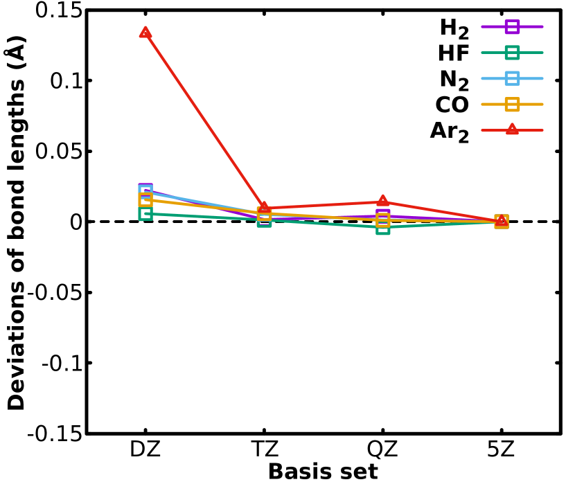
Figure 1: Convergence of the derivations of the RPA@PBE optimized bond lengths from the reference values (obtained at the largest basis set) as a function of the basis set size. For H₂, HF, N₂ and CO, the Gaussian cc-pVXZ basis sets (X=D, T, Q, 5, abbreviated as basis set “DZ”, “TZ”, “QZ”, and “5Z”) are used. For Ar₂, the corresponding aug-cc-pVXZ basis sets are used. The reference RPA@PBE bond lengths at the 5Z level are 0.7428 Å, 0.9216 Å, 1.1044 Å, 1.1366 Å for H₂, HF, N₂ and CO, and 3.7645 Å  for Ar₂, respectively.

Table 3: Comparison of RPA@PBE bond lengths $R_{e}$ (in pm) and bond angles $\varTheta_{e}$ (deg) with those derived from PBE and MP2, obtained using the cc-pVQZ (QZ) basis sets. The RPA geometries obtained using the cc-pV5Z (5Z) basis sets are also presented. For rare gas dimers additional diffuse functions (i.e., aug-cc-pVQZ and aug-cc-pV5Z) are used in the RPA calculations. The reference values are taken from Ref. Pawłowski et al., 2002; Cook et al., 1975; Tang and Toennies, 2003; CCC, 2018 (see text for the actual methods), which are indicated with superscript $a$,  $b$,  $c$  and $d$ respectively. The mean error (ME), mean absolute error (MAE), mean percentage error (MPE) and mean absolute percentage error (MAPE) are presented for each method.

System	$R_{e}/\varTheta_{e}$	Ref.	RPA/QZ	RPA/5Z	PBE	MP2CCC (2018); Aprà et al. (2020)	PBE0
Bond lengths
H2	$R_{e}$	74.15	0.17	0.13	0.87	$-$0.54	0.30
F2	$R_{e}$	141.27	2.40	2.18	0.06	$-$1.56	$-$3.71
N2	$R_{e}$	109.76	0.80	0.68	0.48	1.28	$-$0.86
HF	$R_{e}$	91.68	0.43	0.48	1.25	0.04	0.05
CO	$R_{e}$	112.82	0.94	0.84	0.71	0.64	$-$0.59
CO2	$R_{e}$	116.01	0.93	0.83	1.03	0.61	$-$0.35
HCN	$R_{e}$ (H-C)	106.53	0.38	0.32	0.93	0.11	0.22
	$R_{e}$ (C-N)	115.34	0.77	0.65	0.40	1.02	$-$0.88
HNC	$R_{e}$ (H-N)	99.49	0.32	0.30	1.00	0.86	0.10
	$R_{e}$ (C-N)	116.88	0.87	0.77	0.59	$-$0.05	$-$0.62
C2H2	$R_{e}$ (H-C)	106.17	0.40	0.32	0.82	$-$0.06	0.21
	$R_{e}$ (C-C)	120.36	0.61	0.49	0.28	0.50	$-$0.79
H2O	$R_{e}$ (H-O)	95.80	0.47	0.46	1.08	0.96	$-$0.06
HNO	$R_{e}$ (N-H)	105.20	0.38	0.32	2.90	$-$0.59	0.85
	$R_{e}$ (N-O)	120.86	1.13	1.04	$-$0.12	$-$0.46	$-$1.85
HOF	$R_{e}$ (O-H)	96.87	0.28	0.30	1.07	$-$0.55	$-$0.25
	$R_{e}$ (O-F)	143.45	2.37	2.21	1.02	$-$1.52	$-$2.85
N2H2	$R_{e}$ (H-N)	102.88	0.46	0.41	1.51	$-$0.18	0.25
	$R_{e}$ (N-N)	124.58	1.06	0.91	0.17	0.61	$-$1.53
CH2O	$R_{e}$ (C-O)	120.47	0.77	0.10	0.23	0.35	$-$1.03
	$R_{e}$ (C-H)	110.07	0.37	0.66	1.70	$-$0.15	0.67
C2H4	$R_{e}$ (H-C)	108.07	0.40	0.33	1.02	$-$0.12	0.29
	$R_{e}$ (C-C)	133.07	0.69	0.61	0.15	$-$0.11	$-$0.83
NH3	$R_{e}$ (H-N)	101.24	0.47	0.41	0.92	$-$0.26	$-$0.05
CH4	$R_{e}$ (C-H)	108.59	0.50	0.44	0.94	$-$0.18	0.22
H2S	$R_{e}$ (H-S)	133.56	0.71	0.56	1.67	$-$0.20	0.60
Ne2	$R_{e}$	310.00	11.60	6.82	$-$1.19	9.20	2.38
Ar2	$R_{e}$	375.80	11.26	7.86	10.25	$-$0.40	27.15
Li2	$R_{e}$	267.30	4.37	3.11	4.41	7.30	4.76
BF	$R_{e}$	126.69	0.69	0.62	0.54	$-$0.25	$-$0.77
HCl	$R_{e}$	127.46	0.56	0.47	1.49	$-$0.23	0.44
Cl2	$R_{e}$	198.79	3.82	2.76	2.49	$-$0.26	$-$0.20
$\text{NO}^{+}$	$R_{e}$	106.56	0.62	0.52	0.36	1.30	$-$1.25
BeH2	$R_{e}$	132.64	0.38	0.41	1.03	0.06	0.56
ME	$R_{e}$		1.54	1.16	1.24	0.50	0.61
MAE	$R_{e}$		1.54	1.16	1.31	0.96	1.69
MPD			0.83 %	0.67 %	0.79 %	0.20 %	$-$0.01 %
MAPD			0.83 %	0.67 %	0.96 %	0.58 %	0.85 %
Bond angles
H2O	$\varTheta_{e}$	104.4776∘	$-$1.0008∘	$-$0.7107∘	$-$0.5571∘	$-$0.4648∘	0.2111∘
HNO	$\varTheta_{e}$	108.2600∘	$-$0.3531∘	$-$0.2839∘	0.3952∘	$-$0.4711	0.5308∘
HOF	$\varTheta_{e}$	97.2000∘	$-$0.1241∘	$-$0.0071∘	0.6919∘	0.7962∘	1.8273∘
N2H2	$\varTheta_{e}$	106.3000∘	$-$0.6066∘	$-$0.4516∘	$-$0.0890∘	$-$0.5530∘	0.5167∘
CH2O	$\varTheta_{e}$ (HCO)	121.9330∘	$-$0.0894∘	$-$0.1907∘	0.1857∘	$-$0.1500∘	0.0627∘
	$\varTheta_{e}$ (HCH)	116.1340∘	0.1793∘	0.3812∘	$-$0.3714∘	0.3000∘	$-$0.1254∘
C2H4	$\varTheta_{e}$ (HCC)	121.2000∘	0.2341∘	0.2253∘	0.5096∘	0.1270∘	0.4529∘
	$\varTheta_{e}$ (HCH)	117.6000∘	$-$0.4686∘	$-$0.4498∘	$-$1.0193∘	$-$0.2550∘	$-$0.9057∘
NH3	$\varTheta_{e}$	106.6732∘	$-$1.1347∘	$-$0.7033∘	$-$0.8349∘	$-$0.2090∘	$-$0.0366∘
CH4	$\varTheta_{e}$	109.4710∘	0.0010∘	0.0001∘	0.0000∘	0.0000∘	$-$0.0041∘
H2S	$\varTheta_{e}$	92.1100∘	0.0455∘	0.0633∘	$-$0.3828∘	0.1270∘	0.2117∘
ME	$\varTheta_{e}$		$-$0.3016∘	$-$0.2114∘	0.1338∘	$-$0.0684∘	0.2492∘
MAE	$\varTheta_{e}$		0.3852∘	0.3102∘	0.4579∘	0.3139∘	0.4441∘
MPD	$\varTheta_{e}$		$-$0.29 %	$-$0.18 %	$-$0.06 %	$-$0.06 %	0.26 %
MAPD	$\varTheta_{e}$		0.36 %	0.29 %	0.36 %	0.30 %	0.42 %
aRef. Pawłowski et al.,2002	bRef. Cook et al.,1975	cRef. Tang and Toennies,2003	dRef. CCC,2018

In Table 3 the optimized RPA@PBE equilibrium geometries for 26 small molecules, including both bond lengths and (for poly-atomic molecules) bond angles, are presented. The PBE and MP2 geometries for the same set of molecules are also presented for comparison. As usual, the MP2 calculations are based on the Hartree-Fock reference states and the results are taken from Refs. Aprà et al. (2020); CCC (2018). All calculations are done using the cc-pVQZ basis set (and for rare-gas dimers the aug-cc-pVQZ basis set). For the RPA@PBE results, the cc-pV5Z (and aug-cc-pV5Z for rare-gas dimers) results are also shown, in order to illustrate the basis set effect for RPA geometries for the entire molecular set. The reference geometries used here to benchmark the accuracy of RPA@PBE, PBE, and MP2 are mostly taken from Refs. Pawłowski et al., 2002. These are considered as empirical equilibrium geometries which are determined by a combination of experimental rotational constants and theoretical vibration-rotation interaction constants (at the CCSD(T)/cc-pVQZ) level. The geometry values are believed to be accurate within $0.6\%$, or below 0.1 pm for bond length.

From Table 3, one can see that RPA@PBE systematically overestimates the bond lengths of small molecules, resulting in a MAE of 1.54 pm which is essentially the same as ME, at the cc-pVQZ basis level. It appears that the basis set effect is still appreciable at the cc-pVQZ level: When going to cc-pV5Z, the MAE (and ME) is reduced to 1.16 (1.16) pm. PBE also overestimates the bond lengths on average, but to a lesser extent, with a resultant MAE comparable to RPA@PBE (at the cc-pVQZ level) but a smaller ME. In contrast, the MP2 bond lengths center around the reference values, and do not show such a systematic overestimation behavior as observed for RPA@PBE. Furthermore, the MAE of MP2 (0.96 pm) is also noticeably smaller than those of RPA@PBE and PBE. Close inspection reveals that the RPA@PBE bond lengths of rare-gas dimers Ne₂ and Ar₂, and alkali metal dimer Li₂, and halogen dimers F₂ and Cl₂ have particularly large errors, resulting in an overall moderate performance of RPA@PBE in determining the equilibrium molecular structures. Such observations are consistent with the single-point energy calculations, where RPA was found to systematically underbind molecules and solids, and adding single excitation contributions and second-order screened exchange can largely cure this deficiency Ren et al. (2011); Paier et al. (2012); Ren et al. (2013). Moreover, Table 3 suggests that RPA@PBE tends to overestimate the bond angles. The MAEs of the bond angles of the three methods are comparable, and the accuracy of RPA@PBE bond angles again is improved when increasing the basis set size from cc-pVQZ to cc-pV5Z.

We note that Burow et al. reported in Ref. Burow et al., 2014 a much smaller bond length MAE of 0.45 pm for RPA@PBE. Careful analysis indicates that this discrepancy mainly comes from the different molecular test sets used in the two studies. In Ref. Burow et al., 2014, a subset of 18 molecules was used in the benchmark tests, where in our case 8 additional molecules are included. Especially the newly added molecules such as Ne₂, Ar₂, and Cl₂ have particularly large errors, resulting in the final MAE three times as large for RPA@PBE. In our calculations, including only 18 molecules as those in Ref. Burow et al., 2014, one obtains a MAE of 0.73 pm at the cc-pVQZ level, and 0.64 pm at the cc-pV5Z level. Thus our RPA@PBE error analysis at cc-pV5Z level for a smaller test set is consistent with what is reported in Ref. Burow et al., 2014, using the QZVPPD basis set. In Ref. Rekkedal et al. (2013), Rekkedal et al. also reported a similar MAE of 1.6 pm for RPA bond lengths. However, in the case, the larger MAE can be attributed to the use of Hartree-Fock instead of PBE reference states in their calculations. In summary, we consider our calculations to be a more faithful benchmark for RPA@PBE geometries, due to the enlarged test set and carefully checked basis set convergence behavior.

IV.2 RPA geometries and energy hierarchy for low-lying isomers of water hexamer

Next we employ our analytical RPA force implementation to relax the structures of low-lying isomers of the gas-phase water hexamer. Six water molecules can arrange themselves in a number of different configurations that are very close in energy Hincapié et al. (2010). In particular, the four configurations with lowest energies, known as “prism”, “book”, “cage”, and “cyclic” isomers, differ only by 10-20 meV/H₂O at most in total energy. The correct ordering of the Born-Oppenheimer ground-state energies (i.e., without accounting for zero-point corrections and finite-temperature effect) among these four isomers has been determined by high-level quantum chemistry (MP2 Santra et al. (2008) and CCSD(T) Olson et al. (2007)) approaches as well as diffusion Monte Carlo method Santra et al. (2008). These high-level calculations consistently indicate that the prism isomer is most stable, followed successively by “cage”, “book”, and “cyclic” isomers. However, most semi-local and hybrid density functional approximations (DFAs) are unable to predict the most stable isomer, nor the correct energy ordering of the four isomers Santra et al. (2008). In Ref. Santra et al., 2008, it was explained that the poor treatment of vdW interactions is the key reason for the failure of these functionals. However, it was recently reported that the newly constructed SCAN meta-GGA can yield the correct energy ordering of the four isomers Sun et al. (2016), due to its ability to capture the mid-range vdW interactions.

In this context, it is interesting to check how the RPA performs for describing the structures and energy hierarchy of small water clusters. The RPA is expected to show a better performance than the conventional DFAs in describing the hydrogen-bonded molecular networks, thanks to its ability describing vdW interactions in principle Dobson (1994); Zhu et al. (2010); Ren et al. (2011) and in particular the high-quality vdW coefficients it delivers Gao et al. (2020). We first relax the structures of the four water hexamers using RPA@PBE and cc-pVQZ basis set. The initial geometries for RPA@PBE relaxations were taken from Ref. Wales et al., 2020 for the cage isomer and Ref. Řezáč et al., 2008 for the three other isomers. The structures are relaxed until the RPA@PBE force converges within $10^{-2}$ eV/Å. Once the RPA geometries are obtained, we perform single-point RPA@PBE total energy calculations to determine the dissociation energies for the different isomers, which are defined as

$$D_{e}=-\big{(}E^{\mathrm{RPA}}(\mathrm{(H_{2}O)}_{n})-nE^{\mathrm{RPA}}(\mathrm{H_{2}O)}\big{)}/n\,.$$ (38)

In this definition, a larger positive value of $D_{e}$ means a stronger binding of the water molecules, and that the water cluster is more stable. Since the dissociation energies converge slower than the geometries, here we report results obtained using several different high-quality basis sets, from which one can have a good idea about how well the results are converged with respect to the basis set size. We also note that, to obtain numerically accurate RPA@PBE single point energies, we used additional $5g$ hydrogen-like functions (with effective charge $Z=6$) to generate extra ABFs (the “for_aux” tag in FHI-aims) Ihrig et al. (2015); Ren et al. (2021) to enhance the accuracy of LRI.

Table 4: The RPA@PBE dissociation energies (in meV/H₂O) of the four water hexamer structures obtained using various basis sets, for both relaxed RPA@PBE (upper panel) and PBE (lower panel) geometries. The dissociation energies for the lowest-energy (prism) isomer are highlighted in bold, and the energy differences between other isomers and the lowest-energy ones are indicated in parentheses. Both PBE and RPA@PBE geometries are relaxed using the cc-pVQZ basis set. An additional $5g(Z=6)$ “for_aux” basis function Ihrig et al. (2015) is employed to enhance the accuracy of LRI. The frozen-core approximation is used in all calculations.

Basis Set	Prism	Cage	Book	Cyclic
RPA@PBE geometries
cc-pVQZ	319.5	317.4(2.1)	313.5(6.0)	305.3(14.2)
cc-pV5Z	300.7	299.2(1.5)	297.7(3.0)	292.5(8.2)
NAO-VCC-4Z	300.6	299.5(1.1)	298.1(2.5)	292.2(8.4)
aug-cc-pVQZ	306.6	304.7(1.9)	302.4(4.2)	295.9(10.7)
aug-cc-pV5Z	301.0	299.3(1.7)	297.1(3.9)	290.9(10.1)
CBS(aQZ,a5Z)	295.1	293.6(1.5)	291.5(3.6)	285.7(9.5)
PBE geometries
cc-pVQZ	311.2	307.8(3.4)	302.5(8.7)	293.5(17.7)
cc-pV5Z	291.5	288.3(3.2)	285.0(6.5)	278.7(12.8)
NAO-VCC-4Z	291.8	289.0(2.8)	285.9(5.9)	279.1(12.7)
aug-cc-pVQZ	297.9	294.4(3.5)	290.2(7.7)	282.8(15.1)
aug-cc-pV5Z	291.7	288.2(3.5)	284.1(7.6)	276.5(15.2)
CBS(aQ,a5Z)	285.2	281.7(3.5)	277.7(7.5)	269.9(15.3)

In Table 4 the RPA@PBE dissociation energies for the four water hexamers obtained using Gaussian cc-pVQZ, cc-pV5Z, aug-cc-pVQZ (aQZ), aug-cc-pV5Z (a5Z), and NAO-VCC-4Z Zhang et al. (2013) basis sets are presented. Also presented are the dissociation energies at the complete basis set (CBS) limit, obtained via the two-point extrapolation procedure Helgaker et al. (1997) using aQZ/a5Z data points. Under this procedure, $D_{e}$ at the CBS limit is given by,

$$D_{e}(\text{CBS})=\frac{4^{3}D_{e}(\text{aQZ})-5^{3}D_{e}(\text{a5Z})}{4^{3}-5^{3}}\,.$$ (39)

The basis set superposition error (BSSE) is not corrected in all these calculations, as the BSSE should get diminishingly small as one goes to the CBS limit. For comparison, in addition to the results obtained using the RPA@PBE geometries, we also present the RPA@PBE dissociation energies for the same set of isomers and basis functions using the PBE geometries. First of all, one can see from Table 4 that, for all basis sets, the correct energy ordering of the four isomers is obtained. At the level of 5Z/a5Z, the calculated RPA@PBE dissociation energies differ from their counterparts at the CBS limit by 6-7 meV per H₂O molecule and the energy differences between the isomers differ within 1 meV. Interestingly, results of comparable quality are obtained using the NAO-VCC-4Z basis set Zhang et al. (2013). These are numerical orbitals but generated according to a similar “correlation consistent” principle as the Dunning’s basis sets T. H. Dunning (1989). Here, it seems the $4Z$-level NAO basis set can yield RPA results of comparable quality as the $5Z$ Gaussian basis sets.

As mentioned above, in Table 4, we also investigate the effect of a different geometry (here, the geometry obtained by PBE) on the RPA energies for water hexamer. Compared to the results obtained using the PBE geometries, the RPA dissociation energies obtained using the RPA geometries are bigger in magnitude, meaning that the water clusters settled down in the RPA geometries have lower energies. This is exactly what one would expect, since the RPA geometries are local minima of the RPA potential energy surface, while the PBE geometries are not. Comparing the two sets of results, the water hexamers in their RPA geometries are lower in energy by about 10 meV/H₂O than their counterparts in PBE geometries. The energy differences between the different isomers are noticeably larger in PBE geometries, although the energy ordering among the four isomers does not change. We expect that such structural effects, although not causing a qualitative difference in water hexamers, might have implications for bigger water clusters and bulk water Yao and Kanai (2021).

In Table 5, we compare the RPA@PBE dissociation energies for the four isomers of water hexamer with those obtained by quantum chemistry approaches and conventional DFAs. The RPA@PBE results are obtained in their own geometries and extrapolated to the CBS limit. One can see that the energy differences between different isomers yielded by RPA@PBE are in rather good agreement with the CCSD(T) results. In particular, RPA@PBE seems to show a better performance than MP2, which tends to underestimate the energy differences of the cage, book, and cyclic isomers from the prism isomer. However, RPA@PBE shows a substantial underestimation of the dissociation energies themselves – as large as 50 meV per water molecule. Furthermore, the energy separations between different isomers remain to be underestimated within RPA@PBE, despite its improvement over MP2. The fact that RPA underbinds molecules is well known, and in the past it has been demonstrated that a correction term arising from single excitations helps alleviate this problem Ren et al. (2011); Paier et al. (2012); Ren et al. (2013). In Table 5 we also present the results obtained by RPA plus renormalized single excitations (rSE) correction. It can be seen that RPA+rSE results are in excellent agreement with the CCSD(T) results, both for the dissociation energies and for the energy differences between different isomers.

As post-KS methods, the results of RPA and RPA+rSE necessarily depend on the starting point, i.e., the orbitals and orbital energies generated from a preceding self-consistent field (SCF) calculation. To check this dependence, we performed single-point RPA and RPA+rSE energy calculations based on the hybrid PBE0 Perdew et al. (1996); Ernzerhof and Scuseria (1999) functional using the optimized RPA@PBE geometries. As can be seen from the results presented also in Table 5, the dissociation energies of RPA@PBE0 for the water clusters get larger (correctly) and improve over RPA@PBE. On the contrary, the (RPA+rSE)@PBE0 dissociation energies get smaller compared to their (RPA+rSE)@PBE counterparts, and show a larger derivation from the CCSD(T) results. Nevertheless, the energy differences yielded (RPA+rSE)@PBE0 are still in rather good agreement with the CCSD(T) data. This behavior isn’t surprising, as the magnitude of the rSE correction depends on the preceding SCF reference, owing to the fact that the rSE contribution originates from the difference between exact-exchange and KS exchange potentials Ren et al. (2011, 2013). With hybrid functional starting points, the rSE correction will necessarily get smaller than that with pure local/semilocal functional starting points.

In essence, these benchmark results indicate that RPA+rSE might be a promising affordable approach to study properties of water clusters. In contrast, with the exception of SCAN meta-GGA functional Sun et al. (2016), conventional DFAs, even with vdW corrections, can barely describe the energy hierarchy among different water hexamers, as also indicated in Table 5.

Table 5: Comparison of dissociation energies of the four water hexamers (in meV/H₂O) given by RPA@PBE and various other electronic structure approaches. The RPA@PBE, RPA@PBE0, (RPA+rSE)@PBE and (RPA+rSE)@PBE0 results at the CBS(aQZ,a5Z) limit are obtained in this work. The CCSD(T) results are taken from Ref. Olson et al. (2007) and the results of all other approaches are taken from Ref. Santra et al. (2008). Here the RPA and RPA+rSE energetic calculations are done using RPA@PBE geometries, the CCSD(T) calculations are done using MP2 geometries, and all other types of calculations are done using the geometries generated by the same method. Similar to Table 4, the dissociation energies for the lowest-energy isomer are highlighted in bold, and the energy difference between other isomers and the lowest-energy one are indicated in parentheses.

Method	Prism	Cage	Book	Cyclic
RPA@PBE	295.1	293.6(1.5)	291.5(3.6)	285.7(9.5)
RPA@PBE0	308.5	306.9(1.6)	305.5(3.0)	300.5(8.0)
(RPA+rSE)@PBE	344.5	342.3(2.2)	335.7(8.8)	325.4(19.1)
(RPA+rSE)@PBE0	334.6	332.6(2.0)	329.2(5.4)	321.1(13.5)
MP2b	332.3	331.9(0.4)	330.2(2.1)	324.1(8.2)
CCSD(T)a	347.6	345.5(2.1)	338.9(8.7)	332.5(15.1)
PBEb	336.1(9.5)	339.4(6.2)	345.6	344.1(1.5)
PBE0b	322.9(8.0)	325.3(5.7)	330.9	330.8(0.1)
BLYPb	273.6(16.2)	277.4(12.4)	287.5(2.3)	289.8
PBE+vdWb	377.8(2.3)	380.1	377.8(2.3.)	367.3(12.8)
PBE0+vdWb	360.6(1.3)	361.9	359.2(2.7)	351.4(10.5)
BLYP+vdWb	359.9	359.7(0.2)	356.3(3.6)	344.8(15.1)
aRef Olson et al.,2007		bRef Santra et al.,2008

V Conclusion

In conclusion, we have derived and implemented a formalism for analytical RPA force calculations based on LRI and DFPT. Our current implementation in FHI-aims features a canonical $O(N^{5})$ scaling but a lower scaling is possible by exploiting the sparsity offered by LRI. Benchmark calculations against forces obtained by the finite-difference method and RPA geometries reported in the literature show that our RPA force implementation is highly accurate. By studying the geometries of a representative set of 26 molecules with various bonding characteristics, we found that the usual post-KS RPA approach shows a tendency to systematically overestimate the bond lengths. We then looked at the energy hierarchy of the low-lying isomers of water hexamer, and found that RPA@PBE is able to yield correct energy ordering for the lowest four isomers in both PBE and RPA geometries. However, the energy separations between different isomers are appreciably smaller in their RPA geometries. Finally, by adding the rSE corrections to RPA, both the dissociation energies of the water clusters and their energy differences get substantially improved.

References

- Pulay (1969) P. Pulay, Molecular Physics 17, 197 (1969).
- Feynman (1939) R. P. Feynman, Phys. Rev. 56, 340 (1939).
- Møller and Plesset (1934) C. Møller and M. S. Plesset, Phys. Rev. 46, 618 (1934).
- Ågren (1985) H. Ågren, International Journal of Quantum Chemistry 27, 63 (1985).
- Pople et al. (1979) J. A. Pople, R. Krishnan, H. B. Schlegel, and J. S. Binkley, International Journal of Quantum Chemistry 16, 225 (1979).
- Handy and Schaefer (1984) N. C. Handy and H. F. Schaefer, The Journal of Chemical Physics 81, 5031 (1984).
- Adamowicz et al. (1984) L. Adamowicz, W. D. Laidig, and R. J. Bartlett, International Journal of Quantum Chemistry 26, 245 (1984).
- Stanton (1993) J. F. Stanton, The Journal of Chemical Physics 99, 8840 (1993).
- Stanton and Gauss (1994) J. F. Stanton and J. Gauss, The Journal of Chemical Physics 101, 8938 (1994).
- Bohm and Pines (1953) D. Bohm and D. Pines, Phys. Rev. 92, 609 (1953).
- Gell-Mann and Brueckner (1957) M. Gell-Mann and K. A. Brueckner, Phys. Rev. 106, 364 (1957).
- Langreth and Perdew (1977) D. C. Langreth and J. P. Perdew, Phys. Rev. B 15, 2884 (1977).
- Heßelmann and Görling (2011) A. Heßelmann and A. Görling, Mol. Phys. 109, 2473 (2011).
- Eshuis et al. (2012) H. Eshuis, J. E. Bates, and F. Furche, Theor. Chem. Acc. 131, 1084 (2012).
- Ren et al. (2012a) X. Ren, P. Rinke, C. Joas, and M. Scheffler, J. Mater. Sci. 47, 7447 (2012a).
- van Aggelen et al. (2013) H. van Aggelen, S. N. Steinmann, D. Peng, and W. Yang, Phys. Rev. A 88, 030501(R) (2013).
- Scuseria et al. (2013) E. Scuseria, T. M. Henderson, and I. W. Bulik, J. Chem. Phys. 139, 104113 (2013).
- Yang et al. (2013) Y. Yang, H. van Aggelen, S. N. Steinmann, D. Peng, and W. Yang, J. Chem. Phys. 139, 174110 (2013).
- Peng et al. (2014) D. Peng, H. van Aggelen, Y. Yang, and W. Yang, J. Chem. Phys. 140, 18A522 (2014).
- Tahir and Ren (2019) M. N. Tahir and X. Ren, Phys. Rev. 99, 195149 (2019).
- Rekkedal et al. (2013) J. Rekkedal, S. Coriani, M. F. Iozzi, A. M. Teale, T. Helgaker, and T. B. Pedersen, The Journal of Chemical Physics 139, 081101 (2013).
- Burow et al. (2014) A. M. Burow, J. E. Bates, F. Furche, and H. Eshuis, Journal of Chemical Theory and Computation 10, 180 (2014), pMID: 26579901.
- Ramberger et al. (2017) B. Ramberger, T. Schäfer, and G. Kresse, Phys. Rev. Lett. 118, 106403 (2017).
- Helgaker and Jøgensen (1992) T. Helgaker and P. Jøgensen, in Methods in Computational Molecular Physics, edited by S. Wilson and G. H. F. Diercksen (Plenum Press, Plenum, New York, 1992) pp. 353–421.
- Scuseria et al. (2008) G. E. Scuseria, T. M. Henderson, and D. C. Sorensen, J. Chem. Phys. 129, 231101 (2008).
- Hedin (1965) L. Hedin, Phys. Rev. 139, A796 (1965).
- Liu et al. (2016) P. Liu, M. Kaltak, J. Klimeš, and G. Kresse, Phys. Rev. B 94, 165109 (2016).
- Beuerle and Ochsenfeld (2018) M. Beuerle and C. Ochsenfeld, J. Chem. Phys. 149, 244111 (2018).
- Ihrig et al. (2015) A. C. Ihrig, J. Wieferink, I. Y. Zhang, M. Ropo, X. Ren, P. Rinke, M. Scheffler, and V. Blum, New Journal of Physics 17, 093020 (2015).
- Levchenko et al. (2015) S. V. Levchenko, X. Ren, J. Wieferink, R. Johanni, P. Rinke, V. Blum, and M. Scheffler, Comp. Phys. Comm. 192, 60 (2015).
- Lin et al. (2020) P. Lin, X. Ren, and L. He, J. Phys. Chem. Lett. 11, 3082 (2020).
- Merlot et al. (2013) P. Merlot, T. Kjrgaard, T. Helgaker, R. Lindh, F. Aquilante, S. Reine, and T. B. Pedersen, J. Comput. Chem. 34, 1486 (2013).
- Wirz et al. (2017) L. N. Wirz, S. S. Reine, and T. B. Pedersen, J. Chem. Theory Comput 13, 4897 (2017).
- Baroni et al. (2001) S. Baroni, S. de Gironcoli, A. D. Corso, and P. Giannozzi, Rev. Mol. Phys. 73, 515 (2001).
- Shang et al. (2017) H. Shang, C. Carbogno, P. Rinke, and M. Scheffler, Computer Physics Communications 215, 26 (2017).
- Blum et al. (2009) V. Blum, F. Hanke, R. Gehrke, P. Havu, V. Havu, X. Ren, K. Reuter, and M. Scheffler, Comp. Phys. Comm. 180, 2175 (2009).
- Havu et al. (2009) V. Havu, V. Blum, P. Havu, and M. Scheffler, J. Comp. Phys. 228, 8367 (2009).
- Ren et al. (2012b) X. Ren, P. Rinke, V. Blum, J. Wieferink, A. Tkatchenko, A. Sanfilippo, K. Reuter, and M. Scheffler, New J. Phys. 14, 053020 (2012b).
- Olson et al. (2007) R. M. Olson, J. L. Bentz, R. A. Kendall, M. W. Schmidt, and M. S. Gordon, Journal of Chemical Theory and Computation 3, 1312 (2007).
- Santra et al. (2008) B. Santra, A. Michaelides, M. Fuchs, A. Tkatchenko, C. Filippi, and M. Scheffler, The Journal of Chemical Physics 129, 194111 (2008).
- Dobson (1994) J. F. Dobson, in Topics in Condensed Matter Physics, edited by M. P. Das (Nova, New York, 1994).
- Dunlap et al. (1979) B. I. Dunlap, J. W. D. Connolly, and J. R. Sabin, J. Chem. Phys 71, 3396 (1979).
- Whitten (1973) J. L. Whitten, J. Chem. Phys. 58, 4496 (1973).
- Feyereisen et al. (1993) M. Feyereisen, G. Fitzgerald, and A. Komornicki, Chem. Phys. Lett. 208, 359 (1993).
- Sternheimer (1954) R. M. Sternheimer, Phys. Rev. 96, 951 (1954).
- Knuth et al. (2015) F. Knuth, C. Carbogno, V. Atalla, V. Blum, and M. Scheffler, Computer Physics Communications 190, 33 (2015).
- Aprà et al. (2020) E. Aprà, E. J. Bylaska, W. A. de Jong, N. Govind, K. Kowalski, T. P. Straatsma, M. Valiev, H. J. J. van Dam, Y. Alexeev, J. Anchell, V. Anisimov, F. W. Aquino, R. Atta-Fynn, J. Autschbach, N. P. Bauman, J. C. Becca, D. E. Bernholdt, K. Bhaskaran-Nair, S. Bogatko, P. Borowski, J. Boschen, J. Brabec, A. Bruner, E. Cauë, Y. Chen, G. N. Chuev, C. J. Cramer, J. Daily, M. J. O. Deegan, T. H. Dunning, M. Dupuis, K. G. Dyall, G. I. Fann, S. A. Fischer, A. Fonari, H. Früchtl, L. Gagliardi, J. Garza, N. Gawande, S. Ghosh, K. Glaesemann, A. W. Götz, J. Hammond, V. Helms, E. D. Hermes, K. Hirao, S. Hirata, M. Jacquelin, L. Jensen, B. G. Johnson, H. Jónsson, R. A. Kendall, M. Klemm, R. Kobayashi, V. Konkov, S. Krishnamoorthy, M. Krishnan, Z. Lin, R. D. Lins, R. J. Littlefield, A. J. Logsdail, K. Lopata, W. Ma, A. V. Marenich, J. Martin del Campo, D. Mejia-Rodriguez, J. E. Moore, J. M. Mullin, T. Nakajima, D. R. Nascimento, J. A. Nichols, P. J. Nichols, J. Nieplocha, A. Otero-de-la Roza, B. Palmer, A. Panyala, T. Pirojsirikul, B. Peng, R. Peverati, J. Pittner, L. Pollack, R. M. Richard, P. Sadayappan, G. C. Schatz, W. A. Shelton, D. W. Silverstein, D. M. A. Smith, T. A. Soares, D. Song, M. Swart, H. L. Taylor, G. S. Thomas, V. Tipparaju, D. G. Truhlar, K. Tsemekhman, T. Van Voorhis, A. Vázquez-Mayagoitia, P. Verma, O. Villa, A. Vishnu, K. D. Vogiatzis, D. Wang, J. H. Weare, M. J. Williamson, T. L. Windus, K. Woliński, A. T. Wong, Q. Wu, C. Yang, Q. Yu, M. Zacharias, Z. Zhang, Y. Zhao, and R. J. Harrison, The Journal of Chemical Physics 152, 184102 (2020).
- Rappoport and Furche (2010) D. Rappoport and F. Furche, The Journal of Chemical Physics 133, 134105 (2010), https://doi.org/10.1063/1.3484283 .
- Pawłowski et al. (2002) F. Pawłowski, P. Jørgensen, J. Olsen, F. Hegelund, T. Helgaker, J. Gauss, K. L. Bak, and J. F. Stanton, The Journal of Chemical Physics 116, 6482 (2002).
- Cook et al. (1975) R. L. Cook, F. C. De Lucia, and P. Helminger, Journal of Molecular Structure 28, 237 (1975).
- Tang and Toennies (2003) K. T. Tang and J. P. Toennies, J. Chem. Phys. 118, 4976 (2003).
- CCC (2018) “Nist computational chemistry comparison and benchmark database,” https://cccbdb.nist.gov/ (2018).
- Ren et al. (2011) X. Ren, A. Tkatchenko, P. Rinke, and M. Scheffler, Phys. Rev. Lett. 106, 153003 (2011).
- Paier et al. (2012) J. Paier, X. Ren, P. Rinke, G. E. Scuseria, A. Grüneis, G. Kresse, and M. Scheffler, New J. Phys. 14, 043002 (2012).
- Ren et al. (2013) X. Ren, P. Rinke, G. E. Scuseria, and M. Scheffler, Phys. Rev. B 88, 035120 (2013).
- Hincapié et al. (2010) G. Hincapié, N. Acelas, M. Castaño, J. David, and A. Restrepo, The Journal of Physical Chemistry A 114, 7809 (2010), pMID: 20590081.
- Sun et al. (2016) J. Sun, R. C. Remsing, Y. Zhang, Z. Sun, A. Ruzsinszky, H. Peng, Z. Yang, A. Paul, U. Waghmare, X. Wu, M. L. Klein, and J. P. Perdew, Nature Chemistry 8, 831 (2016).
- Zhu et al. (2010) W. Zhu, J. Toulouse, A. Savin, and J. G. Ángyán, J. Chem. Phys. 132, 244108 (2010).
- Gao et al. (2020) Y. Gao, W. Zhu, and X. Ren, Phys. Rev. B 101, 035113 (2020).
- Wales et al. (2020) D. J. Wales, J. P. K. Doye, A. Dullweber, M. P. Hodges, F. Y. N. F. Calvo, J. Hernández-Rojas, and T. F. Middleton, “The cambridge cluster database,” http://www-wales.ch.cam.ac.uk/~wales/CCD/TIP4P-water.html (2020).
- Řezáč et al. (2008) J. Řezáč, P. Jurečka, K. E. Riley, J. Černý, H. Valdes, K. Pluháčková, K. Berka, T. Řezáč, M. Pitoňák, J. Vondrášek, and P. Hobza, Collection of Czechoslovak Chemical Communications 73, 1261 (2008).
- Ren et al. (2021) X. Ren, F. Merz, H. Jiang, Y. Yao, M. Rampp, H. Lederer, V. Blum, and M. Scheffler, Phys. Rev. Mater. 5, 013807 (2021).
- Zhang et al. (2013) I. Y. Zhang, X. Ren, P. Rinke, V. Blum, and M. Scheffler, New J. Phys. 15, 123033 (2013).
- Helgaker et al. (1997) T. Helgaker, J. Gauss, P. Jørgensen, and J. Olsen, J. Chem. Phys. 106, 6430 (1997).
- T. H. Dunning (1989) J. T. H. Dunning, J. Chem. Phys. 90, 1007 (1989).
- Yao and Kanai (2021) Y. Yao and Y. Kanai, The Journal of Physical Chemistry Letters 12, 6354 (2021).
- Perdew et al. (1996) J. P. Perdew, M. Ernzerhof, and K. Burke, J. Chem. Phys. 105, 9982 (1996).
- Ernzerhof and Scuseria (1999) M. Ernzerhof and G. E. Scuseria, J. Chem. Phys. 110, 5029 (1999).