Regional Adversarial Training for Better Robust Generalization

Abstract

Adversarial training (AT) has been demonstrated as one of the most promising defense methods against various adversarial attacks. To our knowledge, existing AT-based methods usually train with the locally most adversarial perturbed points and treat all the perturbed points equally, which may lead to considerably weaker adversarial robust generalization on test data. In this work, we introduce a new adversarial training framework that considers the diversity as well as characteristics of the perturbed points in the vicinity of benign samples. To realize the framework, we propose a Regional Adversarial Training (RAT) defense method that first utilizes the attack path generated by the typical iterative attack method of projected gradient descent (PGD), and constructs an adversarial region based on the attack path. Then, RAT samples diverse perturbed training points efficiently inside this region, and utilizes a distance-aware label smoothing mechanism to capture our intuition that perturbed points at different locations should have different impact on the model performance. Extensive experiments on several benchmark datasets show that RAT consistently makes significant improvement on standard adversarial training (SAT), and exhibits better robust generalization.

Introduction

Deep learning models have achieved substantial success on a wide variety of computer vision tasks  (He et al. 2016a; Lin et al. 2014; Girshick 2015). However, recent studies have shown that deep learning models are inherently vulnerable to adversarial examples (Szegedy et al. 2014; Goodfellow, Shlens, and Szegedy 2015; Papernot, McDaniel, and Goodfellow 2016; Papernot et al. 2017), i.e., injecting imperceptible but malicious perturbations into the clean input could drastically degrade the model performance.

Adversarial training (AT), which incorporates adversarial examples into the training set, is one of the most effective defense methods to improve the adversarial robustness of deep learning models (Madry et al. 2018; Zhang et al. 2019; Lee, Lee, and Yoon 2020; Athalye, Carlini, and Wagner 2018; Li et al. 2019). However, AT-based defense methods usually suffer from the weak robust generalization due to the following two reasons. Firstly, AT-based methods usually adopt the locally most adversarial perturbed point around each benign data point as the perturbed training point, whereas ignoring the diversity of the perturbed training points and increasing the risk of robust overfitting (Rice, Wong, and Kolter 2020). Secondly, they treat all the perturbed points in the $\epsilon$-ball of the benign points equally, i.e., assigning such points the same one-hot class label of their benign counterparts, but consider neither their characteristics nor differences. Thereby, most existing AT-based methods tend to overfit on the specific attack used in the training and exhibit weak robust generalization for the same threat model with different settings (Tramèr et al. 2018; Song et al. 2019).

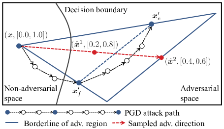
Figure 1: Illustration of the adversarial region and the distance-aware labels for sampled training points. $\bm{x}$ denotes the benign data point. $\bm{x}^{\prime}_{f}$ and $\bm{x}^{\prime}_{e}$ denote the first adversarial point and the end adversarial point along the attack path generated by iterative PGD method, respectively. $\hat{\bm{x}}^{1}$ and $\hat{\bm{x}}^{2}$ are sampled perturbed training points with different soft labels.

To address the aforementioned issues, we propose a new adversarial training framework that advocates exploring the diversity of the perturbed training points and considering their characteristics and differences. We realize this framework by designing a Regional Adversarial Training (RAT) defense method. Firstly, RAT utilizes an Adversarial Region-based Sampler (ARS) for sampling diverse perturbed training points. As illustrated in Figure 1, the adversarial regional sampler first constructs an informative area with three points (the benign data point, the first adversarial point and the end adversarial point along the attack path generated by the typical iterative PGD attack (Madry et al. 2018)), and enlarges the area in an appropriate proportion to obtain the adversarial region. Then, sampling from the adversarial region can boost the diversity of the perturbed training points in terms of adversarial directions and magnitudes. Secondly, RAT proposes a Distance-aware Label Smoothing (DLS) mechanism to capture the intuition that perturbed training points at different locations should have different contributions to the model performance. Specifically, the distance-aware label smoothing mechanism aims to assign different soft labels for perturbed training points based on their characteristics, with the principle that a perturbed point closer to (farther from) the benign point should have higher (lower) confidence w.r.t. the ground-truth class label.

The main contributions of our work are as follows.

• We propose a new adversarial training framework that considers the diversity as well as different characteristics of the perturbed training points in the vicinity of benign samples.

• To realize the framework, we design a Regional Adversarial Training (RAT) defense method that samples diverse perturbed training points in different directions and magnitudes, and assign different soft labels to these perturbed points based on their locations.

• Extensive experiments on three standard datasets validate the superiority of RAT, which consistently makes significant improvements on the standard adversarial training without extra training cost and exhibits better robustness against various adversarial attacks.

• Further analysis show that RAT brings smaller gaps on the standard and adversarial robust generalization, as compared to other AT-based methods, and RAT performs more stably with better robust generalization under the PGD attack with various settings. Moreover, RAT exhibits better robustness on natural image corruptions.

Related Work

Since the discovery of adversarial examples (Goodfellow, Shlens, and Szegedy 2015), various adversarial attack methods have been proposed to deceive deep learning models with small but malicious perturbations. In general, these attack methods can be categorized into two types, i.e., the white-box attacks and the black-box attacks, based on whether the attacker can access the inner information of the target model. Among which, the projected gradient descent method (PGD) (Madry et al. 2018) is a typical white-box iterative attack method.

Correspondingly, numerous methods have been proposed to defense against the adversarial attacks, which can be categorized into input transformation (Buckman et al. 2018; Yang et al. 2019), model ensemble (Pang et al. 2019; Dabouei et al. 2020), and adversarial training (Madry et al. 2018; Zhang et al. 2019; Lee, Lee, and Yoon 2020; Deng et al. 2020). Among which, adversarial training has been demonstrated as one of the most effective methods (Athalye, Carlini, and Wagner 2018; Li et al. 2019; Dong et al. 2020). In the following, we focus on the discussion on adversarial training methods, and clarify how our method differs.

Despite the great success of adversarial training (AT), there remains a visible robust generalization gap between training data and test data. Adversarial training with a specific attack would lead to weak adversarial robust generalization on test data (Zhang et al. 2020; Deng et al. 2020). Moreover, the adversarial robust generalization is theoretically more difficult than standard generalization (Schmidt et al. 2018), and often possesses significantly higher sample complexity (Yin, Ramchandran, and Bartlett 2019; Montasser, Hanneke, and Srebro 2019).

Recently, several AT-based methods have been proposed for improving the adversarial robustness. Zhang et al. (2019) propose TRADES to maximize the trade-off between adversarial robustness and standard accuracy, which is based on the locally most adversarial perturbed points and differs to ours. Lee, Lee, and Yoon (2020) propose the adversarial vertex mixup by augmenting the adversarial examples through mixup operation, but they do not consider the diversity of adversarial directions as we do. They also adopt an existing label-smoothing mechanism (Szegedy et al. 2016) to regularize the classifier, while we design a distance-aware label smoothing (DLS) mechanism that is adaptive for treating the perturbed points differently based on their distances to the benign points.

The most related method to ours is the adversarial distributional training (ADT) (Deng et al. 2020), which trains with a learned adversarial distribution through a neural network to characterize the potential adversarial examples for each benign sample. ADT treats the sampled perturbed training points equally, while we treat the sampled perturbed training points differently based on their characteristics. In addition, modeling the adversarial distribution for each benign point in ADT is intrinsically hard and time-consuming, especially for the high-dimensional image data. While in our method, the sampling of perturbed training points is based on the commonly used PGD attack, therefore as compared with the standard adversarial training, almost no extra attack cost is introduced.

Methodology

We first present the background of the standard adversarial training (SAT) (Madry et al. 2018), then introduce in detail the proposed regional adversarial training (RAT).

Standard Adversarial Training

Given a standard classification task with training dataset $\mathcal{D}=\left\{(\bm{x}_{i},y_{i})\right\}_{i=1}^{n}$ with $c$ classes and $n$ samples, where $\bm{x}_{i}\in\mathbb{R}^{d}$ represents the benign point; $y_{i}\in\left\{1,\dots,c\right\}$ denotes the ground-truth class label, and let $\bm{y}_{i}$ be the one-hot form of the class label $y_{i}$. The standard adversarial training (Madry et al. 2018) is formulated as a min-max optimization problem:

$$\min_{\bm{\theta}}\ \frac{1}{n}\sum_{i=1}^{n}\max_{\bm{x}^{\prime}_{i}\in\mathcal{B}(\bm{x}_{i},\epsilon)}\mathcal{L}(f_{\bm{\theta}}(\bm{x}^{\prime}_{i}),\bm{y}_{i}),$$ (1)

where $f_{\bm{\theta}}(\cdot):\mathbb{R}^{d}\rightarrow\mathbb{R}^{c}$ is the classifier parameterized by $\bm{\theta}$ that outputs the predicted probabilities over all classes; $\mathcal{L}(\cdot,\cdot)$ is the cross-entropy loss; $\mathcal{B}(\bm{x},\epsilon)$ is the $\epsilon$-ball of the benign data point $\bm{x}$, i.e., $\mathcal{B}(\bm{x},\epsilon)=\{\bm{x}^{\prime}:\left\|\bm{x}^{\prime}-\bm{x}\right\|_{\infty}\leq\epsilon\}$. Note that we mainly focus on the $\ell_{\infty}$ threat models to align with previous works.

As formulated in Eq. (1), the inner maximization of the SAT aims to generate the most adversarial perturbed point in set $\mathcal{B}(\bm{x},\epsilon)$ for each benign point, and the outer minimization aims to minimize the cross-entropy loss of all the generated perturbed points. Since the inner maximization does not have a closed-form solution for deep neural networks, a commonly used approximate method is the projected gradient descent (PGD) attack (Madry et al. 2018). Considering a benign sample $(\bm{x},\bm{y})$, the PGD attack updates the adversarial perturbed points with multiple steps:

$$\bm{x}^{\prime}_{t+1}=\Pi_{\mathcal{B}(\bm{x},\epsilon)}\left(\bm{x}^{\prime}_{t}+\alpha\cdot\operatorname{sign}\left(\nabla_{\bm{x}^{\prime}_{t}}\mathcal{L}(f_{\theta}(\bm{x}^{\prime}_{t}),\bm{y})\right)\right),$$ (2)

where $\bm{x}^{\prime}_{t}$ is the perturbed point at the $t$-th step; $\Pi_{\mathcal{B}(\bm{x},\epsilon)}(\cdot)$ is the function to project the inputs into the allowed set $\mathcal{B}(\bm{x},\epsilon)$; $\alpha>0$ is the step size of PGD attack. $\bm{x}^{\prime}_{0}$ is randomly sampled from $\mathcal{B}(\bm{x},\epsilon)$.

By revisiting the formulation of SAT in Eq. (1), on one hand, we see that SAT always optimizes on the locally most adversarial perturbed point within the $\epsilon$-ball, overlooking the diversity of perturbed training points. Actually, for each benign data point, there usually exist multiple adversarial directions and magnitudes that could lead to successful attack. On the other hand, for the outer minimization of SAT, all the perturbed training points are treated equally and assigned the same one-hot class label of their benign counterparts, while their characteristics are not utilized during the training.

Regional Adversarial Training

In this work, we explore the diversity of perturbed training points and treat them differently based on their characteristics. In general, our adversarial training framework could be expressed as:

$$\begin{gathered}\min_{\bm{\theta}}\ \frac{1}{n\times m}\sum_{i=1}^{n}\sum_{j=1}^{m}\mathcal{L}(f_{\bm{\theta}}(\hat{\bm{x}}_{i}^{j}),\hat{\bm{y}}_{i}^{j})),\\ \end{gathered}$$ (3)

where

$$\begin{gathered}\hat{\bm{y}}_{i}^{j}=S_{L}(\hat{\bm{x}}_{i}^{j},\bm{y}_{i}).\end{gathered}$$ (4)

Here $\hat{\bm{x}}_{i}^{j}$ denotes the diverse perturbed training points for the benign sample $(\bm{x}_{i},\bm{y}_{i})$, where $j=1,...,m$; $S_{L}(\hat{\bm{x}}_{i}^{j},\bm{y}_{i})$ is the soft label assignment function for assigning representative soft labels to the perturbed training point $\hat{\bm{x}}_{i}^{j}$ based on their characteristic.

To realize this framework, we propose a new defense method called Regional Adversarial Training (RAT). Firstly, in order to enrich the diversity of the perturbed training points, we propose an efficient Adversarial Region-based Sampler (ARS), where we construct an adversarial region around each benign data point based on the attack path of the PGD method, and sample perturbed training points with various directions and magnitudes inside this region. Secondly, we capture the intuition that perturbed training points at different locations should have different contributions to the model performance. Thus we propose a Distance-aware Label Smoothing (DLS) mechanism that assigns different smoothing factors to each perturbed training point based on their distance to the benign point. In this way, our adversarially trained models make significant improvements on SAT, and exhibit better robust generalization.

In the following, we introduce in detail how ARS and DLS work, as well as the overall training procedure.

Adversarial Regional Sampler.

To enrich the perturbed training points, one simple method is to generate a set of adversarial examples by performing PGD attack with various settings for multiple times. But it will significantly increase the training cost, especially for large-scale datasets. Thus, we propose an efficient adversarial region-based sampler (ARS) to obtain diverse perturbed training points.

To describe ARS more clearly, we define the first adversarial point $\bm{x}_{f}^{\prime}$ and the end adversarial point $\bm{x}_{e}^{\prime}$ of the PGD attack as follows.

Definition 1 (First / End Adversarial Point)

Let $S(x)=\{\bm{x}_{t}^{\prime}\}_{t=1}^{K}$ indicates the attack sequence of the benign sample $(\bm{x},y)$ generated by a $K$-step PGD attack. Assuming there exists at least one adversarial perturbed point that leads to a successful attack, the end adversarial point is defined as $\bm{x}^{\prime}_{e}\triangleq\bm{x}_{K}^{\prime}$, and the first adversarial point is defined as $\bm{x}^{\prime}_{f}\triangleq\bm{x}_{t}^{\prime}$, where $t=\arg\min_{t}(\phi(f_{\bm{\theta}}(\bm{x}_{t}^{\prime}))\neq y)$, and $\phi(\cdot)$ is the function to obtain the predicted label from output probability.

In most cases, there will be at least one or two adversarial points along the path during the PGD process. Without loss of generality, we assume there exists at least one successful perturbed point along the PGD attack sequence.

As illustrated in Figure 1, we construct a region with three points (the benign data point $\bm{x}$, the first adversarial point $\bm{x}^{\prime}_{f}$ and the end adversarial point $\bm{x}^{\prime}_{e}$ along the PGD attack path). We observe that, firstly, starting from $\bm{x}$ to any point on the line segment between $\bm{x}^{\prime}_{f}$ and $\bm{x}^{\prime}_{e}$, this region essentially provides diverse adversarial directions. Secondly, we could expand the region along the adversarial directions to construct a larger adversarial region for capturing richer perturbed points and sample multiple perturbed points with different magnitudes along each adversarial direction inside the adversarial region.

Based on the above observations, we propose the adversarial region-based sampler (ARS). ARS first randomly samples a point $\bar{\bm{x}}$ on the line segment between $\bm{x}^{\prime}_{f}$ and $\bm{x}^{\prime}_{e}$ to determine the adversarial direction ($\bm{x}$ to $\bar{\bm{x}}$). Then, ARS samples a perturbed training point $\hat{\bm{x}}$ with a magnitude scale factor $s$ along this direction. The sampling process is formulated as follows:

$$\begin{gathered}\bar{\bm{x}}=\lambda\cdot\bm{x}^{\prime}_{f}+(1-\lambda)\cdot\bm{x}^{\prime}_{e},\ \lambda\sim\mathcal{U}(0,1),\\ \hat{\bm{x}}=\bm{x}+s\cdot(\bar{\bm{x}}-\bm{x}),\ s\sim\mathcal{S},\end{gathered}$$ (5)

where $\lambda$ is uniformly sampled in [0,1]; $s$ is the scale factor to control the adversarial magnitude, i.e., the distance to the benign point $\bm{x}$. We define the magnitude scale factor from the benign sample $\bm{x}$ to the line segment formed by $\bm{x}^{\prime}_{f}$ and $\bm{x}^{\prime}_{e}$ is $1$. The magnitude scale factor $s$ is randomly picked from the scale candidate set $\mathcal{S}$, which consists of multiple scale factors varying from $0$ to $S(S=2$ or 3 in our experiments). A larger scale factor $s$ indicates that the sampled perturbed training point $\hat{\bm{x}}$ is farther away from the corresponding benign point $\bm{x}$. When $s$ is 0, the sampled perturbed point $\hat{\bm{x}}$ coincides with the benign point $\bm{x}$. When $s$ is 1, $\hat{\bm{x}}$ lies in the farthest bound of the expanded adversarial region.

In this way, for each training iteration of RAT, ARS only needs to perform the PGD attack once to generate the perturbed training points with diverse directions and magnitudes, and no extra attack cost is imposed as compared to the standard adversarial training.

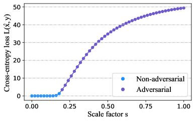
Figure 2: Visualization of the cross-entropy loss and attack result for the perturbed point $\hat{\bm{x}}$ sampled in a selected adversarial direction with various magnitude scale factor $s$. Here Adversarial denotes successful attack, and Non-adversarial denotes unsuccessful attack.

Distance-aware Label Smoothing.

Directly adopting the one-hot class label of the benign samples to train with diverse perturbed points may overlook their characteristics and differences, leading to the underutilization of the diversity. Our intuition is that a perturbed point closer to the benign point should have higher confidence w.r.t. the ground-truth class label, and vise versa.

To verify our intuition, we randomly pick a correctly classified sample $(\bm{x},\bm{y})$ on CIFAR-10, and then sample the perturbed point $\hat{\bm{x}}$ with multiple magnitudes along the randomly selected direction. We visualize the cross-entropy loss and attack results of the perturbed point $\hat{\bm{x}}$ in Figure 2. It shows that the cross-entropy loss increases as the magnitude scale factor $s$ increases, which demonstrates our intuition.

Based on the above observations, we propose the distance-aware label smoothing (DLS) mechanism to treat the perturbed training points sampled from ARS differently. Considering a perturbed training point $\hat{\bm{x}}$ sampled based on Eq. (5), the corresponding distance-aware soft label $\hat{\bm{y}}$ is formally defined as follows:

$$\begin{gathered}\hat{\bm{y}}=S_{L}(\hat{\bm{x}},\bm{y})=\bm{y}\cdot\beta+(1-\bm{y})\cdot\frac{1-\beta}{c-1},\end{gathered}$$ (6)

where

$$\begin{gathered}\beta=\beta_{max}-s\times\frac{\beta_{max}-\beta_{min}}{S}.\end{gathered}$$ (7)

$\bm{y}$ is the one-hot ground-truth class label of the benign point $\bm{x}$; $c$ is the number of classes, and $s$ is the magnitude scale factor for the perturbed point $\hat{\bm{x}}$ in Eq. (5); $S$ is the maximal magnitude scale factor inside the adversarial region; $\beta$ is the label smoothing factor determined by the scale factor $s$; $\beta_{max}$ and $\beta_{min}$ are the maximal and minimal label-smoothing factors, respectively. As can be seen in Eq. (7), a larger scale factor $s$ can lead to a smaller label smoothing factor $\beta$, and a lower confidence w.r.t. the ground-truth class label $y$ for the perturbed training point $\hat{\bm{x}}$. As shown in Figure 1, compared to $\hat{\bm{x}}^{1}$, the sampled perturbed point $\hat{\bm{x}}^{2}$ farther away from the benign point $\bm{x}$ has a lower confidence w.r.t the ground-truth class label.

Overall Training Procedure.

The overall training procedure of RAT is summarized in Algorithm 1. During the training, RAT first obtains the attack path for each benign point based on the PGD attack. Then, RAT samples multiple perturbed training points with random adversarial directions and magnitudes based on ARS. Third, RAT assigns such perturbed training points with the distance-aware soft labels based on DLS. In the end, RAT computes the loss of the perturbed training samples and updates the model parameters $\bm{\theta}$ with the gradient on loss.

Overall, the framework of RAT facilitates a more reasonable learning scheme for adversarial training by considering the diversity and characteristics of the perturbed training points. Note that the standard adversarial training is a special case of RAT, by specifying the $\bm{x}^{\prime}_{f}\triangleq\bm{x}^{\prime}_{e}$ for the adversarial region, the scale factor $s=1$ for the adversarial regional sampler, and the label smoothing factors $\beta_{min}=\beta_{max}=1.0$ for the distance-aware label smoothing mechanism.

Algorithm 1 Regional Adversarial Training (RAT)

0:  Network $f_{\bm{\theta}}$, training dataset $\mathcal{D}$, training epochs $T$, number of batches $M$, batchsize $n$, learning rate $\eta$ and the number of samples $m$

1:  for epoch = $1,...,T$ do

2:     for mini-batch = $1,...,M$ do

3:        Sample a mini-batch $\{(\bm{x}_{i},\bm{y}_{i})\}^{n}_{i=1}\sim\mathcal{D}$

4:        for $i=1$ to $m$ (in parallel) do

5:           Generate multiple perturbed training points and their distance-aware soft labels $\{(\hat{\bm{x}}_{i}^{j},\hat{\bm{y}}_{i}^{j})\}_{j=1}^{m}$ for $(\bm{x}_{i},\bm{y}_{i})$ by Eq. (5) and Eq. (6)

6:        end for

7:        $\bm{\theta}\leftarrow\bm{\theta}-\eta\cdot\frac{1}{n\times m}\sum_{i=1}^{n}\sum_{j=1}^{m}\nabla_{\bm{\theta}}\mathcal{L}(f_{\bm{\theta}}(\hat{\bm{x}}^{j}_{i}),\hat{\bm{y}}^{j}_{i})$

8:     end for

9:  end for

9:  robust network $f_{\bm{\theta}}$

Experiments

To evaluate the robustness and generalization ability of the proposed RAT, we present experimental results on various datasets and models. All image values are normalized into $[0,1]$. All experiments are run on a single NVIDIA Tesla V100 GPU.

Baseline Methods. We compare RAT with the following training methods: standard training (ST), standard adversarial training (SAT) (Madry et al. 2018), TRADES (Zhang et al. 2019), adversarial vertex mixup (AVM) (Lee, Lee, and Yoon 2020), and adversarial distributional training (ADT) (Deng et al. 2020). We adopt $\lambda$ = 6 for TRADES, and adopt ADT_EXP version for ADT as reported in the original paper for the best performance.

Datasets. We use three benchmark datasets including CIFAR-10 (Krizhevsky et al. 2009), CIFAR-100 (Krizhevsky et al. 2009), and a subset of ImageNet called ImageNette (Howard 2019). CIFAR-10 and CIFAR-100 are widely adopted by adversarial training studies including the baseline methods. For the large-scale ImageNet dataset, just as all the baseline methods did not report the results, we are also unable to evaluate on ImageNet due to the very high training cost. Still, we add a comparison on ImageNette, a subset of ImageNet.

Training Setup. For the neural networks, we choose WRN-34-10 (Zagoruyko and Komodakis 2016) for the experiments on CIFAR, and PreActResNet18 (He et al. 2016b) for the experiments on ImageNette. For fair comparisons, we follow the training settings as in (Madry et al. 2018; Lee, Lee, and Yoon 2020), and train the models using SGD with 0.9 momentum for $80k$ steps with the initial learning rate of 0.1, but divided by 10 at the step $30k$ and $45k$, respectively. The batch size is 128 and the weight decay is $2\times 10^{-4}$. For the generation of adversarial examples, the perturbation bound $\epsilon$ = 8/255; the PGD iteration number $K$ = 10; and the PGD step size $\alpha$ = 2/255. For the hyperparameters of RAT, we set the scale factor set $\mathcal{S}$ as $\{0.0,0.1,0.2,...,2.0\}$ for CIFAR and $\{0.0,0.1,0.2,...,3.0\}$ for ImageNette, the number of samples $m$ = 2, and the maximal and minimal label-smoothing factors are set to 1.0 and 0.1, respectively.

Model	Clean	FGSM	PGD	CW∞	$\mathcal{N}$attack
CIFAR-10 (The perturbation bound $\epsilon=8/255$).
ST	95.42	12.91	0.00	0.00	0.00
SAT	86.92	55.58	47.74	48.64	47.20
TRADES	85.84	59.23	50.39	51.02	50.30
AVM	92.40	76.92	62.19	56.83	58.00
ADT	87.98	58.25	49.27	50.38	47.60
RAT	93.17	77.51	70.57	65.54	69.70
CIFAR-100 (The perturbation bound $\epsilon=8/255$).
ST	78.75	6.99	0.00	0.00	0.00
SAT	60.03	28.27	24.34	23.95	26.50
TRADES	57.64	29.80	26.43	25.25	27.40
AVM	69.48	52.95	29.53	24.00	30.90
ADT	62.63	29.94	24.53	25.04	27.10
RAT	70.65	57.16	37.03	27.45	40.70
ImageNette (The perturbation bound $\epsilon=8/255$).
ST	89.02	7.80	0.00	0.00	0.00
SAT	83.52	57.76	53.58	52.92	50.90
TRADES	82.52	58.01	53.73	53.25	52.20
AVM	87.87	58.55	50.14	45.22	54.10
ADT	78.83	56.05	52.99	51.82	51.50
RAT	86.19	74.75	61.83	55.82	59.60

Table 1: Test accuracy (%) of RAT and the baselines under the white-box and black-box attacks on CIFAR-10, CIFAR-100 and ImageNette. Clean denotes the standard accuracy.

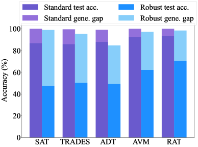
Figure 3: Standard and adversarially robust generalization gaps of RAT and the baselines on CIFAR-10.

Evaluation Setup. We report both the standard accuracy on clean data, and the robust accuracy on adversarial examples. Following the widely adopted protocol (Madry et al. 2018; Zhang et al. 2019), we consider the white-box attacks including FGSM (Goodfellow, Shlens, and Szegedy 2015), PGD (Madry et al. 2018) and CW_∞ (Carlini and Wagner 2017) , and the black-box attack, $\mathcal{N}$attack (Li et al. 2019). For PGD and CW_∞, the perturbation bound $\epsilon$ = 8/255; the step number $K$ = 10; and the step size $\alpha$ = 2/255, which keep the same as in the training setting. For the $\mathcal{N}$attack, we perform on a subset of 1,000 randomly selected test images due to the high complexity for query, and set the maximum iteration number to 200 and sample 300 perturbations at each iteration.

Evaluation Results

We first validate our main intuitions: by considering the diversity and characteristics of the perturbed training points, is it possible to develop the robust models that show better robust generalization?

As shown in Table 1, we report the standard and robust test accuracy of RAT and the baselines on three standard datasets. Clearly, RAT achieves the best adversarial robustness against both white-box and black-box attacks, and maintains high standard test accuracy on various datasets. For example, on CIFAR-10 dataset, RAT outperforms the robust accuracy of the SAT baseline by a large margin of 22.83% under the PGD attack, meanwhile RAT outperforms the standard accuracy of SAT by a clear margin of 6.25%. These results indicate that, by considering the diversity and characteristics of the perturbed training points, RAT could significantly improve the robust generalization of SAT, verifying that the framework behind RAT is more suitable for adversarial training.

Further Analysis on RAT

We conduct a series of additional analysis on the robust generalization of RAT.

Comparison on Generalization Gaps. We first analyze the standard and adversarial robust generalization gaps for RAT and the baseline defense methods. The standard generalization gap is defined as the difference of the standard accuracy between training data and test data, and similarly, the adversarial robust generalization gap is defined as the difference of the robust accuracy on the PGD attack between training data and test data. The results on CIFAR-10 dataset are reported in Figure 3. We have similar results on CIFAR-100 and ImageNette, as reported in the supplementary material. These results consistently demonstrate that RAT can bring smaller gaps on the standard and adversarial robust generalization, as compared to other AT-based methods.

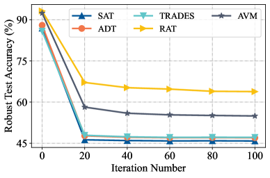
Figure 4: Robust test accuracy (%) of RAT and the baselines against PGD with various iterations on CIFAR-10. The PGD perturbation budget is 8/255 and the PGD step size is 2/255.

Robustness against PGD with Various Iterations and Perturbation Budgets. 1) As shown in Figure 4, we visualize the robust accuracy of RAT and the baselines under the PGD attack with the iteration number $K$ varying from 0 to 100, where the perturbation budget is 8/255 and the step size is 2/255. The robust accuracy of all the defense methods first decreases and then stabilizes as the iteration number increases. RAT consistently outperforms all the baselines under various iteration numbers, and outperforms the second best by a clear margin of around 10% after 20 steps of PGD iterations. 2) As shown in Figure 5, we visualize the robust accuracy against PGD with the perturbation budget varying from 0 to 16/255, where the step size is 2/255 and the iteration number is 10. The robust accuracy of all the defense methods decreases along with the increasing perturbation budget. However, RAT exhibits stronger adversarial robustness, and the difference is much clearer for higher perturbation budgets. We have similar results on CIFAR-100 and ImageNette, as reported in the supplementary material. These results consistently indicate that RAT can achieve better robust generalization on the PGD attack with different iteration numbers and perturbation budgets.

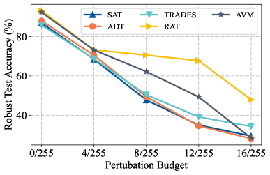
Figure 5: Robust test accuracy (%) of RAT and the baselines against PGD with various perturbation budgets on CIFAR-10. The PGD step size is 2/255, the iteration number is 10.

Model	mCA	Blur Corruptions				Weather Corruptions				Digital Corruptions
		Defocus	Glass	Motion	Zoom	Snow	Frost	Fog	Bright	Contrast	Elastic	Pixelate	JPEG
CIFAR-10-C
ST	81.15	83.40	53.27	79.51	77.23	83.57	82.03	90.59	94.42	92.68	84.18	75.72	77.19
SAT	81.58	83.05	79.97	80.02	82.20	82.40	85.26	71.70	86.70	76.38	81.13	85.07	85.06
TRADES	80.67	82.34	79.02	79.32	81.41	81.00	84.22	71.13	85.83	75.80	80.24	83.94	83.80
AVM	87.05	88.52	82.67	85.24	87.57	86.98	89.50	81.29	91.85	84.12	86.91	89.99	89.96
ADT	77.36	82.76	80.30	78.32	81.59	81.49	78.51	62.54	84.52	45.67	81.50	85.66	85.51
RAT	87.94	89.12	83.25	85.75	88.45	87.90	90.15	83.04	92.76	85.70	87.95	90.35	90.86
CIFAR-100-C
ST	57.45	62.73	21.30	58.27	57.47	56.63	52.75	69.95	75.46	71.89	61.79	54.13	46.98
SAT	52.87	54.84	50.85	51.30	53.13	52.80	56.76	41.80	59.07	47.26	52.30	57.59	56.71
TRADES	50.99	52.89	50.15	49.57	51.60	51.04	54.81	39.64	57.26	44.85	50.26	55.35	54.47
AVM	61.48	63.77	55.37	59.51	62.39	61.26	64.46	52.62	67.75	57.68	61.38	65.75	65.86
ADT	50.79	55.97	52.69	51.56	54.75	53.37	49.66	34.80	57.99	25.37	54.30	60.02	59.04
RAT	62.44	64.20	55.39	59.84	62.70	62.20	65.71	54.55	69.27	59.92	62.00	67.30	66.21

Table 2: Classification accuracy (%) of RAT and the baselines on the commonly occurring natural image corruptions of CIFAR-10-C and CIFAR-100-C. The mCA refers to the mean accuracy averaged on different corruptions and severities.

Model	Clean	PGD	CW∞
SAT	86.92	47.74	48.64
SAT+ARS	87.67	52.59	50.87
SAT+ARS+DLS	93.17	70.57	65.34

Table 3: Ablation study for the impact of ARS and DLS.

Method	$\beta_{max}$	$\beta_{min}$	Clean	PGD	CW∞
RAT	1.0	0.1	90.94	70.57	65.54
	1.0	0.3	92.59	64.87	61.53
	1.0	0.5	91.55	62.86	56.95
	0.8	0.1	92.33	66.44	63.47
	0.6	0.1	91.65	62.93	59.88

Table 4: Test accuracy (%) of the training framework RAT with different maximal label-smoothing factor $\beta_{max}$ and minimal label-smoothing factor $\beta_{min}$ on CIFAR-10.

Robustness against Natural Image Corruptions. Recent works (Gilmer et al. 2019; Yin et al. 2019) found that adversarial training may harm the robustness against natural image corruptions, as compared with standard training. Therefore, to further investigate the performance of RAT, we consider to quantify the robustness under the natural image corruptions. Specifically, we consider the benchmark datasets CIFAR-10-C (Hendrycks and Dietterich 2019) and CIFAR-100-C (Hendrycks and Dietterich 2019) that consists of various types of natural image corruptions. We select 12 types of common image corruptions, including blur corruptions, weather corruptions and digital corruptions. For each type of corruptions, there are five levels of severity.

As shown in Table 2, we report the average accuracy of all the five levels of severity for CIFAR-10-C and CIFAR-100-C, respectively. We can easily see that RAT leads to better robustness under a wide range of natural image corruptions, and outperforms all the baselines in terms of the average accuracy over all corruptions. The evaluations indicate that RAT can prevent the models from overfitting to certain attacking patterns, and exhibits better robust generalization on natural image corruptions.

Identifying Obfuscated Gradients. Here we further show that RAT does not lead to the obfuscated gradients (Athalye, Carlini, and Wagner 2018; Li et al. 2019) as RAT does not fit the following characteristics defined by  Athalye, Carlini, and Wagner (2018) and  Gilmer et al. (2018) that models with obfuscated gradients may suffer.

1) One-step attacks perform better that iterative attacks perform. On the contrary, extensive evaluations in Table 1 indicate that under the defense of RAT, stronger iterative attacks (e.g., PGD and CW_∞) are more powerful than the single-step attack (e.g., FGSM). 2) Robustness under white-box setting is higher than that under black-box setting. The results of RAT in Table 1 and Figure 4 show that, the stronger iterative white-box attacks are more successful than black-box attacks, which contradicts the model’s gradient being obfuscating. 3) A higher distortion bound increases the defense robustness. Conversely, the evaluation in Figure 5 shows that the robustness of RAT decreases with the increase of the perturbation budget.

Computation Efficiency. The time cost of adversarial training is mainly caused by the attack overhead. RAT only needs to execute one PGD attack in each training iteration, thus RAT does not introduce extra attack cost as compared with SAT. For instance, on CIFAR-10, the running time of 1000 training iterations is $41.88$ minutes for SAT and $47.95$ minutes for RAT, thus little training cost is introduced for each training iteration of RAT.

Ablation Studies

To gain further insights on the performance of RAT, we delve into RAT to investigate the impact of various components (i.e., the adversarial regional sampler (ARS) and the distance-aware label smoothing (DLS)) on CIFAR-10. We report the standard accuracy and the robust accuracy over the PGD, CW_∞ attacks for each model.

Impact of ARS and DLS. Since DLS is dependent with ARS in RAT, we train the models of SAT, the combination of SAT+ARS, and the combination of SAT+ARS+DLS (i.e., RAT) following the same training setting in Section Experiments, to show the impact of ARS and DLS. As shown in Table 3, we can see that SAT+ARS exhibits great improvements on SAT over both the standard accuracy and the robust accuracy, which indicates considering the diversity of the perturbed training points does help promote the adversarial robustness without the degradation of standard accuracy. After further combining SAT+ARS with DLS, we can see that DLS further takes the advantage of ARS, and yields more improvements on SAT, which demonstrates that treating the perturbed training points based on their characteristics can achieve better robust generalization.

Selection of Maximal and Minimal Label-smoothing Factors. Different selections of the maximal and minimal label-smoothing factors ($\beta_{max}$ and $\beta_{min}$) in RAT lead to different trade-offs between the standard accuracy and the adversarial robustness of the trained models, as shown in Table 4. Such trade-off is prevalent w.r.t. the hyperparameter settings in various adversarial training frameworks (Madry et al. 2018; Zhang et al. 2019; Deng et al. 2020). Besides, RAT makes steady improvements for different maximal and minimal label-smoothing factors in a wide range.

Conclusion

To boost the adversarially robust generalization, we explore a new adversarial training framework that considers the diversity as well as characteristics of the perturbed points in the neighborhood of benign samples, and implement our idea by proposing a Regional Adversarial Training (RAT) defense method. The key components of RAT are the adversarial region-based sampler (ARS) that aims to consider the sampling diversity, and the distance-aware label smoothing (DLS) that aims to treat the sampled perturbed training points differently based on their characteristics. Extensive experiments show that RAT could efficiently enhance the adversarial robustness without extra training cost as compared with the standard adversarial training, and performs favorably against state-of-the-art defenses in terms of standard accuracy and adversarial robustness. RAT also performs more stably with better robustness on the PGD attack with various settings and natural image corruptions, as compared to other AT-based methods.

Appendix

We report more experimental results on the CIFAR-100 and ImageNette datasets below, including the comparison on generalization gaps, and the robustness against PGD with various iterations and perturbation budgets.

Comparison on Generalization Gaps. Similar to the evaluation on CIFAR-10 in the main submission, we analyze the standard and adversarially robust generalization gaps for RAT and the baseline defense methods on the CIFAR-100 and ImageNette datasets. We report the analysis results of the CIFAR-100 and ImageNette datasets in Figure 6. The results consistently demonstrate that RAT can bring smaller gaps on the standard and adversarially robust generalization, as compared to other AT-based methods.

Robustness against PGD with Various Iterations. As shown in Figure 7, we visualize the robust accuracy under the PGD attack with the iteration number $K$ varying from 0 to 100 on the CIFAR-100 and ImageNette datasets, respectively. The perturbation budget is 8/255 and the step size is 2/255. The robust accuracy of all the defense methods first decreases and then stabilizes as the iteration number increases. The proposed RAT consistently outperforms all the baselines under various iteration numbers, which indicates that RAT can achieve better robust generalization on the PGD attack with different number of iterations.

Robustness against PGD with Various Perturbation Budgets. In Figure 8, we evaluate the model robustness under the PGD attack with the perturbation budget $\epsilon$ varying from 0 to 16/255, on CIFAR-100 and ImageNette, respectively. The step size is 2/255 and the iteration number is 10. The robust accuracy of all the defense methods decreases along with the increasing of the perturbation budget. However, RAT exhibits stronger adversarial robustness, and the superiority is much clearer for higher perturbation budgets. These results consistently verify that RAT can achieve better adversarially robust generalization on the PGD attack with different perturbation budgets.

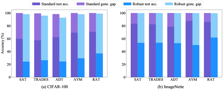
Figure 6: Standard and adversarially robust generalization gaps of RAT and the baselines on CIFAR-100 and ImageNette.

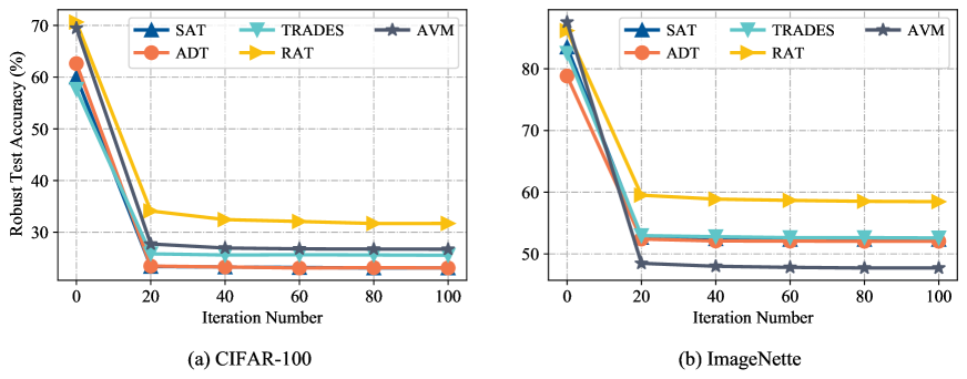
Figure 7: Robust test accuracy (%) of RAT and the baselines against PGD with various iterations on CIFAR-100 and ImageNette. The PGD perturbation budget is 8/255 and the PGD step size is 2/255.

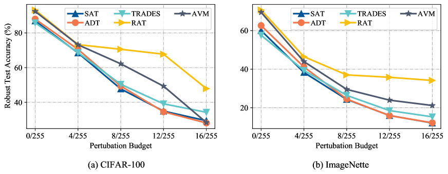
Figure 8: Robust test accuracy (%) of RAT and the baselines against PGD with various perturbation budgets on CIFAR-100 and ImageNette. The PGD step size is 2/255 and the PGD iteration number is 10.

References

- Athalye, Carlini, and Wagner (2018) Athalye, A.; Carlini, N.; and Wagner, D. A. 2018. Obfuscated Gradients Give a False Sense of Security: Circumventing Defenses to Adversarial Examples. In ICML, 274–283.
- Buckman et al. (2018) Buckman, J.; Roy, A.; Raffel, C.; and Goodfellow, I. 2018. Thermometer encoding: One hot way to resist adversarial examples. In ICLR.
- Carlini and Wagner (2017) Carlini, N.; and Wagner, D. 2017. Towards evaluating the robustness of neural networks. In IEEE S&P, 39–57.
- Dabouei et al. (2020) Dabouei, A.; Soleymani, S.; Taherkhani, F.; Dawson, J.; and Nasrabadi, N. M. 2020. Exploiting Joint Robustness to Adversarial Perturbations. In CVPR, 1122–1131.
- Deng et al. (2020) Deng, Z.; Dong, Y.; Pang, T.; Su, H.; and Zhu, J. 2020. Adversarial Distributional Training for Robust Deep Learning. In NeurIPS.
- Dong et al. (2020) Dong, Y.; Fu, Q.-A.; Yang, X.; Pang, T.; Su, H.; Xiao, Z.; and Zhu, J. 2020. Benchmarking Adversarial Robustness on Image Classification. In CVPR, 321–331.
- Gilmer et al. (2018) Gilmer, J.; Adams, R. P.; Goodfellow, I. J.; Andersen, D. G.; and Dahl, G. E. 2018. Motivating the Rules of the Game for Adversarial Example Research. CoRR, abs/1807.06732.
- Gilmer et al. (2019) Gilmer, J.; Ford, N.; Carlini, N.; and Cubuk, E. D. 2019. Adversarial Examples Are a Natural Consequence of Test Error in Noise. In ICML.
- Girshick (2015) Girshick, R. 2015. Fast r-cnn. In ICCV, 1440–1448.
- Goodfellow, Shlens, and Szegedy (2015) Goodfellow, I. J.; Shlens, J.; and Szegedy, C. 2015. Explaining and Harnessing Adversarial Examples. In ICLR.
- He et al. (2016a) He, K.; Zhang, X.; Ren, S.; and Sun, J. 2016a. Deep residual learning for image recognition. In CVPR, 770–778.
- He et al. (2016b) He, K.; Zhang, X.; Ren, S.; and Sun, J. 2016b. Identity mappings in deep residual networks. In ECCV, 630–645.
- Hendrycks and Dietterich (2019) Hendrycks, D.; and Dietterich, T. G. 2019. Benchmarking Neural Network Robustness to Common Corruptions and Perturbations. In ICLR.
- Howard (2019) Howard, F. J. 2019. The imagenette dataset. https://github.com/fastai/imagenette.
- Krizhevsky et al. (2009) Krizhevsky, A.; et al. 2009. Learning multiple layers of features from tiny images.
- Lee, Lee, and Yoon (2020) Lee, S.; Lee, H.; and Yoon, S. 2020. Adversarial Vertex Mixup: Toward Better Adversarially Robust Generalization. In CVPR, 272–281.
- Li et al. (2019) Li, Y.; Li, L.; Wang, L.; Zhang, T.; and Gong, B. 2019. NATTACK: Learning the Distributions of Adversarial Examples for an Improved Black-Box Attack on Deep Neural Networks. In ICML, 3866–3876.
- Lin et al. (2014) Lin, T.-Y.; Maire, M.; Belongie, S.; Hays, J.; Perona, P.; Ramanan, D.; Dollár, P.; and Zitnick, C. L. 2014. Microsoft coco: Common objects in context. In ECCV, 740–755.
- Madry et al. (2018) Madry, A.; Makelov, A.; Schmidt, L.; Tsipras, D.; and Vladu, A. 2018. Towards Deep Learning Models Resistant to Adversarial Attacks. In ICLR.
- Montasser, Hanneke, and Srebro (2019) Montasser, O.; Hanneke, S.; and Srebro, N. 2019. VC Classes are Adversarially Robustly Learnable, but Only Improperly. In COLT.
- Pang et al. (2019) Pang, T.; Xu, K.; Du, C.; Chen, N.; and Zhu, J. 2019. Improving Adversarial Robustness via Promoting Ensemble Diversity. In ICML, 4970–4979.
- Papernot, McDaniel, and Goodfellow (2016) Papernot, N.; McDaniel, P. D.; and Goodfellow, I. J. 2016. Transferability in Machine Learning: from Phenomena to Black-Box Attacks using Adversarial Samples. CoRR, abs/1605.07277.
- Papernot et al. (2017) Papernot, N.; McDaniel, P. D.; Goodfellow, I. J.; Jha, S.; Celik, Z. B.; and Swami, A. 2017. Practical Black-Box Attacks against Machine Learning. In AsiaCCS, 506–519.
- Rice, Wong, and Kolter (2020) Rice, L.; Wong, E.; and Kolter, J. Z. 2020. Overfitting in adversarially robust deep learning. arXiv preprint arXiv:2002.11569.
- Schmidt et al. (2018) Schmidt, L.; Santurkar, S.; Tsipras, D.; Talwar, K.; and Madry, A. 2018. Adversarially Robust Generalization Requires More Data. In NeurIPS, 5019–5031.
- Song et al. (2019) Song, C.; He, K.; Wang, L.; and Hopcroft, J. E. 2019. Improving the Generalization of Adversarial Training with Domain Adaptation. In ICLR.
- Szegedy et al. (2016) Szegedy, C.; Vanhoucke, V.; Ioffe, S.; Shlens, J.; and Wojna, Z. 2016. Rethinking the inception architecture for computer vision. In CVPR, 2818–2826.
- Szegedy et al. (2014) Szegedy, C.; Zaremba, W.; Sutskever, I.; Bruna, J.; Erhan, D.; Goodfellow, I. J.; and Fergus, R. 2014. Intriguing properties of neural networks. In ICLR.
- Tramèr et al. (2018) Tramèr, F.; Kurakin, A.; Papernot, N.; Goodfellow, I. J.; Boneh, D.; and McDaniel, P. D. 2018. Ensemble Adversarial Training: Attacks and Defenses. In ICLR.
- Yang et al. (2019) Yang, Y.; Zhang, G.; Xu, Z.; and Katabi, D. 2019. ME-Net: Towards Effective Adversarial Robustness with Matrix Estimation. In ICML, 7025–7034.
- Yin et al. (2019) Yin, D.; Lopes, R. G.; Shlens, J.; Cubuk, E. D.; and Gilmer, J. 2019. A Fourier Perspective on Model Robustness in Computer Vision. In NeurIPS.
- Yin, Ramchandran, and Bartlett (2019) Yin, D.; Ramchandran, K.; and Bartlett, P. L. 2019. Rademacher Complexity for Adversarially Robust Generalization. In ICML.
- Zagoruyko and Komodakis (2016) Zagoruyko, S.; and Komodakis, N. 2016. Wide residual networks. arXiv preprint arXiv:1605.07146.
- Zhang et al. (2019) Zhang, H.; Yu, Y.; Jiao, J.; Xing, E. P.; Ghaoui, L. E.; and Jordan, M. I. 2019. Theoretically Principled Trade-off between Robustness and Accuracy. In ICML, 7472–7482.
- Zhang et al. (2020) Zhang, J.; Xu, X.; Han, B.; Niu, G.; Cui, L.; Sugiyama, M.; and Kankanhalli, M. 2020. Attacks Which Do Not Kill Training Make Adversarial Learning Stronger. In ICML.