Classifying Anomalies THrough Outer Density Estimation (CATHODE)

Abstract

We propose a new model-agnostic search strategy for physics beyond the standard model (BSM) at the LHC, based on a novel application of neural density estimation to anomaly detection. Our approach, which we call Classifying Anomalies THrough Outer Density Estimation (Cathode), assumes the BSM signal is localized in a signal region (defined e.g. using invariant mass). By training a conditional density estimator on a collection of additional features outside the signal region, interpolating it into the signal region, and sampling from it, we produce a collection of events that follow the background model. We can then train a classifier to distinguish the data from the events sampled from the background model, thereby approaching the optimal anomaly detector. Using the LHC Olympics R&D dataset, we demonstrate that Cathode nearly saturates the best possible performance, and significantly outperforms other approaches that aim to enhance the bump hunt (CWoLa Hunting and Anode). Finally, we demonstrate that Cathode is very robust against correlations between the features and maintains nearly-optimal performance even in this more challenging setting.

I Introduction

While there is compelling theoretical and experimental motivation for new physics to be discovered at the Large Hadron Collider (LHC), it is not possible to perform a dedicated search for every conceivable scenario. The ATLAS [1, 2, 3], CMS [4, 5, 6], and LHCb [7] collaborations have extensive search programs for new physics, but there are more models to search for than can be covered by individual analyses. Even searches for pairs of particles are largely unexplored [8, 9], in part because of the theory space priors guiding analysis development. The lack of discoveries thus far could therefore be because existing searches do not cover the anomalous regions of phase space. As a result, it is essential to complement the search program with methods that are more model agnostic.

While some traditional searches for physics beyond the standard model (BSM) provide an interpretation with little dependence on a particular signal model, most searches are optimized with a limited set of benchmarks. Only a relatively small number of searches are signal model independent from the start, including analyses that focus on single features (e.g. bump hunts) and more multivariate searches that compare data with simulation in a large number of signal regions [10, 11, 12, 13, 14, 15, 16, 17, 18, 19, 20, 21, 22, 23].

Recent innovations in machine learning have resulted in powerful new techniques for model agnostic searches in high energy physics. These anomaly detection approaches employ a variety of strategies to be broadly sensitive to new physics with varying methods for modeling the standard model background. In addition to community challenges such as the LHC Olympics [59] and DarkMachines [70], these tools have also been applied for the first time to collider data by the ATLAS Collaboration [74].

An important class of anomaly detection strategies builds on the bump hunt. The traditional bump hunt assumes that a potential signal is localized in one known feature $m$ (often an invariant mass) and then uses data away from the signal (sideband region or SB) to estimate the background. This setup is sketched in Fig. 1. The exact location of the signal (signal region or SR) is scanned over $m$. While broadly sensitive to new physics models with the targeted resonance and nearly independent of simulation for the background modeling, bump hunts are not particularly sensitive to any BSM model. Machine learning approaches that enhance the bump hunt use features $x$ other than $m$ to automatically amplify the presence of a potential signal. The ultimate goal is to approximate the likelihood ratio between the background and the data in the signal region,

$$R(x)={p_{\rm data}(x)\over p_{\rm bg}(x)}$$ (1)

as this is the optimal test statistic for a data-versus-background hypothesis test [75].

Figure 1: Schematic view of the bump hunt. The signal (blue) is localized in the signal region (SR). The background (red) is estimated from a sideband region (SB).

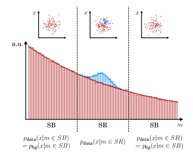
Multiple strategies have been proposed for this task. One approach is based on the Classification Without Labels (CWoLa) protocol [76, 25, 26] in which one trains a classifier to distinguish the SR and SB data. One of the biggest challenges with the CWoLa Hunting approach is its high sensitivity to correlations between the features $x$ and $m$. Multiple variations of CWoLa Hunting have been proposed to circumvent the correlation challenge, such as Simulation Assisted Likelihood-free Anomaly Detection (Salad) [38] and Simulation-Assisted Decorrelation for Resonant Anomaly Detection (SA-CWoLa) [52].

An alternative approach is to learn the two likelihoods directly and then take the ratio. This is the core idea behind Anomaly Detection with Density Estimation (Anode) [39]. The SB is used to estimate $p_{\text{bg}}(x|m)$ for the background (assuming little signal contamination outside the SR). This likelihood is then interpolated into the SR. Combined with an estimate of $p_{\text{data}}(x|m)$ trained in the SR, one can construct an estimate of the likelihood ratio. The SB interpolation makes Anode robust to correlations between $x$ and $m$, although density estimation is inherently more challenging than classification.

In this paper, we propose a new method which combines the best of CWoLa Hunting and Anode. With Classifying Anomalies THrough Outer Density Estimation (Cathode), we train a density estimator to learn the (usually smooth) background distribution in the SB which we refer to as the “outer” region. Then we interpolate it into the SR, but rather than directly constructing the likelihood ratio as in Anode (which would require us to also separately learn $p_{\text{data}}(x|m)$ in the SR), we instead generate sample events from the trained, interpolated background density estimator. These sample events should follow $p_{\text{bg}}(x|m)$ in the SR. Finally, we train a classifier (as in CWoLa Hunting) to distinguish $p_{\text{data}}(x|m)$ from $p_{\text{bg}}(x|m)$ in the SR.

Using the R&D dataset [77] from the LHC Olympics (LHCO) [59], we will show that Cathode achieves a level of performance (as measured by the significance improvement characteristic) that greatly surpasses both CWoLa Hunting and Anode, across a wide range of signal cross sections. Cathode easily outperforms Anode because it does not have to directly learn $p_{\text{data}}$ in the SR, and in particular does not have to learn the sharp increase in $p_{\text{data}}$ where the signal is localized in all of the features. Meanwhile, it outperforms CWoLa Hunting because of a combination of two effects: one is that in Cathode, we can oversample the outer density estimator, leading to more background events than CWoLa Hunting has access to (CWoLa Hunting is limited to the actual data events in the sideband region), and yielding a more powerful classifier. Secondly, the features are slightly correlated with $m$ in the LHCO R&D dataset, and this slightly degrades the performance of CWoLa Hunting, while Cathode is robust.

We also compare Cathode to a fully supervised classifier (i.e. trained on labeled signal and background events) and an “idealized anomaly detector” (trained on data vs. perfectly simulated background). The latter places an upper bound on the performance of any data-vs-background anomaly detection technique, and we show how Cathode essentially saturates its performance. This means that for the first time, a fully-simulation-independent anomaly detection method has been demonstrated to achieve the theoretical upper bound in sensitivity to new physics. The Cathode method is basically the best that it could possibly be.

Finally, as in [39], we study the case where $x$ and $m$ are correlated, by adding artificial linear correlations to two of the features in $x$. Again we show that Cathode (like Anode, and unlike CWoLa Hunting) is largely robust against such correlations, and continues to match the performance of the idealized anomaly detector.

In this work, we will concern ourselves solely with signal sensitivity, and reserve the problem of background estimation for future study. As long as the Cathode classifier does not sculpt features into the invariant mass spectrum, it should be straightforward to combine it with a bump hunt in $m$.

This paper is organized as follows: Section II briefly introduces the LHCO dataset and our treatment of it, and Section III describes the steps of the Cathode approach in detail. Results are given in Section IV and we conclude with Section V. In Appendix A, we provide details of the other approaches (CWoLa Hunting, Anode, idealized anomaly detector and fully supervised classifier) considered in this paper. A further study of correlated features is given in Appendix B.

II The dataset

For the most part, our treatment of the data (background and signal processes, features, signal and sideband regions) follows [39] closely. Here we will briefly review these choices and also highlight some important differences.

We use QCD dijet events as SM background and $W^{\prime}\rightarrow X(\rightarrow qq)Y(\rightarrow qq)$ events as signal, where $m_{W^{\prime}}=3.5~{}$TeV, $m_{X}=500~{}$GeV and $m_{Y}=100~{}$GeV. These are taken from the original LHCO R&D dataset [77]. They are simulated using Pythia 8 [78, 79] and Delphes 3.4.1 [80, 81, 82]. The reconstructed particles of each event are clustered into $R=1$ anti-$k_{T}$ [83] jets using Fastjet [84, 85]; all events are required to satisfy a single $p_{T}>1.2$ TeV jet trigger.

The training features are based on observables constructed by the two highest-$p_{T}$ jets. The two jets are sorted by their invariant mass, such that $m_{J_{1}}<m_{J_{2}}$. The input features used are: the invariant mass of the two jet system ($m_{JJ}$), the invariant mass of the lighter jet, the difference in the invariant masses ($\Delta m_{J}=m_{J_{2}}-m_{J_{1}}$), and the $n$-subjettiness ratios $\tau_{21}^{J_{1}}$ and $\tau_{21}^{J_{2}}$. The $n$-subjettiness ratios are defined as $\tau_{ij}\equiv\tau_{i}/\tau_{j}$ [86, 87].

The signal and sideband regions for the enhanced bump hunt will be defined in terms of the invariant mass of the system: $m_{JJ}\in[3.3,\,\,3.7]$ TeV for the signal region (SR) and its complement $m_{JJ}\notin[3.3,\,\,3.7]$ TeV for the sideband (SB) region. For simplicity, we will specialize to a single $m_{JJ}$ window in this paper, optimally centered on the location of the signal. In practice, as with any other (enhanced) bump hunt method, one would imagine scanning the SR across the entire $m_{JJ}$ range and including appropriate trial factors.

Figure 2: Visualization of the events and how they are split into datasets. The number of signal (sg) and background (bg) events in each dataset is given. Note that “simulation” and “evaluation” are only in the SR, so there are some signal events in the SB that are not used at all.

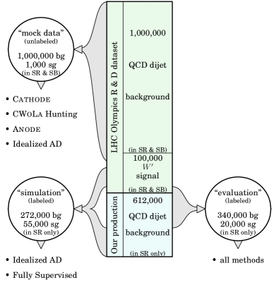
In this work we will compare the Cathode method against a variety of both simulation-independent anomaly detection (CWoLa Hunting, Anode) and simulation-dependent methods. The simulation-dependent methods will be highly idealized, in the sense that our simulations of background and signal will be assumed to be perfect. Accordingly, we must be very careful about the separation between what we consider as the “data”, i.e. events that would come from an experiment in an actual application of the methods; vs. the “simulation”, i.e. events that would be simulated even in a real world application. Figure 2 visualizes our datasets (see also Table 1 for more details).

• For the mock data, we use all of the 1,000,000 SM background events, together with 1,000 (or fewer) signal events, from the original LHCO R&D dataset. All of the simulation-independent anomaly detection methods will be trained and validated (model selection) using the mock data alone.

• Of the remaining 99,000 signal events in the original LHCO R&D dataset, approximately 75,000 lie within the SR. For simulation events, we reserved 55,000 of these. For background, we generated an additional 272,000 QCD dijet events specifically in the SR (so with $m_{JJ}\in[3.3,3.7]$ TeV) using the same settings, trigger and data format as the original LHCO R&D dataset. The fully supervised classifier uses both signal and background simulation events, while the idealized anomaly detector only uses background.

• Finally we set aside some signal and background events for the common evaluation of all of the methods. These events were not touched during the training or validation of any of the methods. We used the remaining 20,000 SR signal events from the original LHCO R&D dataset, together with an additionally generated set of 340,000 QCD dijet events in the SR.

For our primary benchmark mock dataset (1M background events and 1k signal events), there are 121,352 background events and 772 signal events in the signal region, corresponding to an initial $S/B=6\times 10^{-3}$ and $S/\sqrt{B}=2.2$. This is the same benchmark studied in [39] and approximately the same signal vs. background composition as Black Box 1 of the LHC Olympics 2020 [59]. The purpose of this choice is to ensure that (a) the signal is not too numerous such that a conventional bump hunt in $m_{JJ}$ would already result in a discovery of the signal (obviating the need for any sophisticated anomaly detection method); yet (b) not too few that no anomaly detection method would ever succeed in discovering the signal amongst the background.

In order to probe this most interesting regime of signal strengths relevant for anomaly detection techniques, we will also perform a scan over different levels of $S/B$ in this work, and we will see the point at which all of the anomaly detection methods fail.

III The CATHODE method

III.1 Conditional density estimation

The first step of the Cathode method is to train a conditional density estimator on the outer data. Assuming the signal is mostly contained in the SR (as it is here), then the density estimator will learn $p_{\text{data}}(x|m\notin{\rm SR})\approx p_{\text{bg}}(x|m\notin{\rm SR})$, where $m=m_{JJ}$ and $x=\left(m_{J_{1}},\,\,\Delta m_{J},\,\,\tau_{21}^{J_{1}},\,\,\tau_{21}^{J_{2}}\right)$.

In this work, we focus on a single baseline density estimator: the Masked Autoregressive Flow (MAF) with affine transformations [88]. This was used previously in Ref. [39] and was found to perform well on the LHCO R&D dataset. (See also Ref. [58] for another density estimator that performed well on this dataset.) As in [39], we will use a base distribution consisting of the unit normal. In a subsequent publication [89] we will compare and contrast different methods for conditional density estimation. For a description of MAFs and normalizing flows more generally, we refer the reader to Refs. [39, 90] or to reviews in the ML literature [91, 92].

As in Ref. [39], the features are shifted and scaled to the range $x\in(0,1)$, logit transformed, and finally standardized by subtracting the mean and dividing by the standard deviation of the training set before being passed to the density estimator. This transformation was chosen since it improves the accuracy of the density estimator by turning regions of difficulty (typically sharp edges) into smooth tails, which are easier to learn.

The mock data in the SB region is split into a training set consisting of 500,000 events, and a validation set consisting of the remaining SB events in the mock data (378,876 to be precise). The validation set is reserved for model selection.

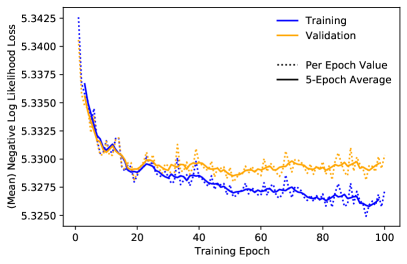
The MAF density estimator is trained using PyTorch [93] in the SB region for 100 epochs with the Adam optimizer [94], a learning rate $10^{-4}$, batch size 256, and batch normalization with a momentum of 1.0. It consists of 15 MADE blocks, with each block consisting of one hidden layer of 128 nodes. This is the same configuration as used in [39]. The training loss and validation loss are tracked throughout training for each epoch. The ten epochs (model states) with the lowest validation loss are selected for the next step of the Cathode method (interpolation and sampling). Since the global minima are used, these 10 epochs do not need to be consecutive.

The loss curves for one such MAF training are shown as dotted lines in Fig. 3, with the moving averages of 5 epochs in solid lines.

Figure 3: Training and validation loss for the MAF (dotted lines) and the 5 epoch moving average (solid lines)

III.2 Interpolation and sampling

The next step of the Cathode method is to interpolate the conditional density estimator trained on the SB region into the SR and then sample events from it. We now describe this process in more detail.

Exactly the same as in the Anode method [39], this interpolation is automatically handled by the MAF. While the MAF was trained on events with $m\notin{\rm SR}$ to learn a bijective, invertible map $z=f(x;m)$ between the 4d features $x$ and latent space $z$ following the base distribution (unit normal), this function can be queried for any value of $m$, including $m\in{\rm SR}$. In Anode, $f$ was used for density estimation, but here we use its inverse $x=f^{-1}(z;m)$ to produce samples in $x$ following the background distribution in the SR.

A sample of $N$ events are generated from each of the 10 chosen model states. The events are then combined and shuffled into a set of $10N$ sample points. This ensembling procedure gives a more representative set of samples than a single model would. In Sec. IV.4, we will explore the role that $N$ plays in the quality of the anomaly detection task, and the potential benefits of oversampling the background model in the SR.

Since we want the sampled synthetic background data to follow the actual data distribution as closely as possible, when sampling we use a matching set of $10N$ $m$ values drawn from the same distribution as the data. To learn the $m$ distribution of the SR data, we perform a kernel density estimate (KDE) fit to the $m$ values in the training set. The KDE was implemented using the Scikit-learn library [97] with a gaussian kernel and a bandwidth of 0.01. To be fully explicit: every sample we produce proceeds from $f^{-1}(z;m)$ with $z\sim{\mathcal{N}}(0,1)^{4}$ and $m\sim p_{KDE}(m)$.

Since the mock data is logit transformed and standardized before being passed to the density estimator, the sampled events are also produced in this transformed and standardized space. They are brought back to the physical space by applying the inverses of the standardization and logit transform, using the SB model parameters (as these were the parameters used by the density estimator). Note that the physical space here refers to the 4d feature space $x=\left(m_{J_{1}},\,\,\Delta m_{J},\,\,\tau_{21}^{J_{1}},\,\,\tau_{21}^{J_{2}}\right)$ and does not include $m$ by construction; sampling from $m$ occurs through the separate KDE step described above.

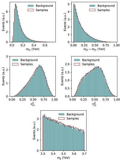
The resulting distributions of the sampled events and the mock data background in the validation dataset are shown in Fig. 4. One can see that there is a notable overlap between the two distributions in all auxiliary features, as well as on the $m$ distribution drawn from the KDE fit.

Figure 4: Normalized distributions of the features of the actual background and of the synthetic samples.

III.3 Classifier

The third step of the Cathode method is to train a classifier to distinguish the generated sample events (that should follow the background distribution in the SR) from the mock data (that follow the background plus signal distribution in the SR). For all the variations we will explore (including CWoLa Hunting), we will use the same classifier architecture. This consists of 3 hidden layers with 64 nodes each and a binary cross-entropy loss.

The binary classifier, also implemented with PyTorch [93], is trained for 100 epochs with a batch size of 128, using the Adam [94] optimizer with a learning rate of $10^{-3}$. When the classes are imbalanced (as will be the case when we oversample the background model), they are reweighted in the loss computation accordingly, such that they contribute equally. Note that here classes refer to the sampled events and the mock data, not signal and background events.

For this step, we divide the mock data in the SR in half, reserving 60,000 events for training the classifier and the remaining 60,000 events for validation (model selection). In a real-life application one would want to perform $k$-fold cross validation so as to not throw away half of the events. However, as this is a proof of concept we do not employ this here.

Unless stated otherwise, we sample in total 400,000 events from the MAF generative model (so $N=40,000$ in the description of Section III.2), which are distributed equally (200,000 each) into the training and validation set for the classifier. Different choices will then be compared in Section IV.4.

Before the mock data and sampled events are passed on to the classifier, the features are re-standardized, this time using the mean and standard deviation of the SR data features. Here, a logit transformation is not used as it has consistently resulted in sub-optimal anomaly detection performance.

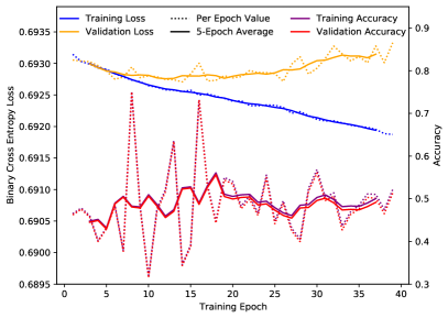
During training, the loss is recorded on the validation set, as shown in Fig. 5. The model states of the 10 epochs with the lowest validation losses are used to construct an ensemble prediction. As in the density estimator ensemble, these epochs do not need to be consecutive. In the ensembling, the individual predictions of each data point are averaged. Since the loss is defined with respect to labels indicating whether a data point is from mock data or sampled events, this approach does not rely on any truth information pertaining to the anomaly.

Figure 5: Training and validation loss of the classifier (dotted lines) and the 5 epoch moving average (solid lines) during training. The accuracy is also shown, which in the case of low signal contamination should oscillate around 0.5 if the two classes are indistinguishable.

III.4 Anomaly detection

The final step of Cathode is to apply the trained classifier to the data in the SR. Recall from the discussion in the introduction that the ultimate goal of an optimal anomaly detector is to learn the likelihood ratio $R(x)$ between the data and background, see Eq. (1). In the presence of an anomaly, we will have

$$p_{\rm data}(x)=f_{\rm bg}p_{\rm bg}(x)+f_{\rm sig}p_{\rm sig}(x)\,,$$ (2)

with a $f_{\rm sig}=1-f_{\rm bg}\ll f_{\rm bg}$ signal (anomaly) fraction. Although this signal fraction is unknown (along with the form of $p_{\rm sig}(x)$), the likelihood ratio $R(x)=p_{\rm data}(x)/p_{\rm bg}(x)$ is nevertheless monotonic with the signal-to-background likelihood ratio. Therefore, if the Cathode method works, the events that are tagged by the classifier as “data-like” should be signal enriched, regardless of the signal.

In the following section, we will demonstrate the efficacy of the Cathode method on the LHCO R&D dataset. Our performance metric will be the significance improvement characteristic (SIC). The SIC curve is defined as the signal efficiency ($\epsilon_{S}$) divided by the square root of the background efficiency ($\epsilon_{B}$), plotted versus the signal efficiency. The background and signal efficiencies are defined based off of a cut on the classifier score. It is important to note that obtaining the SIC curve is only possible through the use of the underlying truth labels available in the LHCO R&D dataset. Thus, this performance metric is only a means to demonstrate the ability to find a signal in the data if it were present. In practice, one would have to calculate the $p$-value under the background-only hypothesis, while selecting events through the use of Cathode and a suitable background estimation procedure (e.g. sideband interpolation as in the bump hunt).

As described in Section II, in order to improve the statistical significance of these efficiencies, we choose to evaluate all methods on a common test set consisting of 340,000 background events and 20,000 signal events in the SR. This test set is reserved from the outset of the analysis and is never used for the training or validation of any of the methods.

IV Results

We first present the results of the Cathode method on the original LHCO features, and then we examine the effect of additional correlations between the features.

Besides Cathode, we will also include the performance of several other methods: CWoLa Hunting [25, 26]; Anode [39]; an “idealized” anomaly detector and a fully supervised classifier. For more details of these methods, see the descriptions in the Introduction and in Appendix A. The idealized anomaly detector, being a classifier between the data and a perfectly simulated background model, sets an upper bound on the performance of any weakly-supervised anomaly detection method that attempts to learn the likelihood ratio between data and background events. Meanwhile, the supervised classifier is trained on labeled background vs. signal events. This method sets an absolute upper bound on the performance of any search strategy focused on this signal hypothesis.

IV.1 Performance on the original LHCO R&D dataset

Figure 6: Background rejection (left) and significance improvement (right) of the various anomaly classifiers as a function of the signal efficiency. The solid lines are deduced from a median value of 10 fully independent trainings on the same training, validation and evaluation set. The uncertainty bands quantify the variance from retraining the NNs on the same, fixed dataset and are defined such that they contain 68% of the runs around the median.

Figure 7: Left: Median maximum significance improvement of each method with 10 different signal injections (leading to a different split of training, validation and evaluation sets in each run) at each decreasing value of signal/background ratios. Here, the 68% hatched uncertainty bands quantify the variance (around the median) from both retrainings of the NN and random realizations of the training and validation data, including different realizations of the 1,000 injected signal events. Right: Achieved maximum significance, which is computed by multiplying the uncut significance by the maximum significance improvement. Both plots feature the significance without any cut applied in the upper horizontal axis. The dotted lines on the right hand side denote 3 and 5 $\sigma$ significance values.

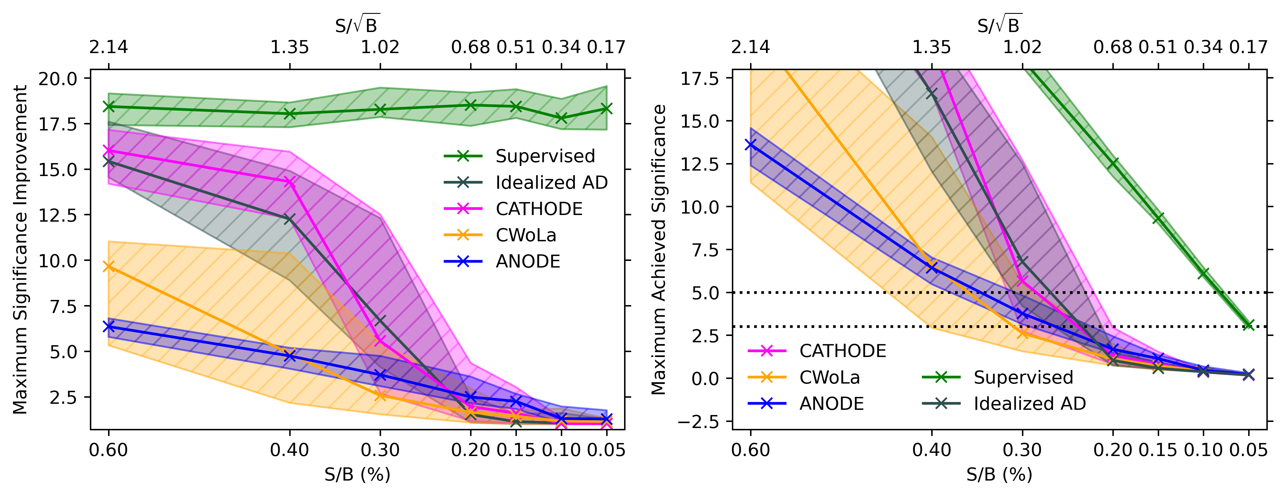
Figure 6 shows the receiver operating characteristic (ROC) curves and the SIC curves of the different anomaly detection methods trained on our baseline dataset. As described in Section II, this consists of 1000 signal events injected into the full background sample, of which 772 are in the SR. The curves in Fig. 6 show the median value and 68% confidence bands of 10 independent trainings, where all steps of each method (e.g. both density estimator and classifier for Cathode) have been reinitialized in each run. Note that, at this stage, we do not explore the variance due to different realizations of the signal or background events (e.g. different choices of the 1000 signal events in the mock data); later in this section, when we explore the performance at smaller $S/B$, the effect of this variation will be included.

We see that overall, Cathode outperforms the other weakly supervised methods across a wide range of signal efficiencies — a factor of more than 2 compared to Anode and a factor of 1.3–2 compared to CWoLa Hunting. At lower signal efficiencies, Cathode reaches a maximum SIC of 14, which represents a significant improvement compared to Anode’s 6.5 and CWoLa Hunting’s 11. A more detailed comparison of Cathode with the other methods is as follows:

• Both Cathode and Anode need to learn the smoothly varying background. However, Anode must also learn the sharply peaked distributions in $x$ where the signal is localized (the “inner” density estimator trained on the SR). This results in a degradation of the Anode anomaly detection method and worse performance than Cathode and CWoLa Hunting.

• As for how Cathode is able to outperform CWoLa Hunting, there are two reasons. Firstly, there is a correlation at the percent level between the chosen features in $x$ within the original LHCO R&D dataset with the search variable ($m_{JJ}$). Since CWoLa Hunting is very sensitive to correlations, this small correlation is sufficient to degrade the performance compared to that of Cathode. Details of the correlation study can be found in Sec. IV.3. Secondly, CWoLa Hunting is limited to only using the events within the sidebands to train the classifier (approximately 65,000 events), while Cathode is able to oversample events from the background model (here 200,000 events are used). These additional events for training allow for a significant performance enhancement of the Cathode method. Further details on the effects of oversampling are studied in Sec. IV.4.

• Next we turn to the comparison between Cathode and the simulation-dependent methods. Recall that the idealized anomaly detector is meant to provide an upper bound on the performance of any data vs. background anomaly detection method. Therefore, it is remarkable that Cathode achieves essentially the same performance as the idealized anomaly detector. The nearly optimal sensitivity of the Cathode method to the signal in the LHCO R&D dataset indicates that interpolated density estimator is modeling the background in the SR with very high fidelity.

• Finally, we see from Fig. 6 that while Cathode and the idealized anomaly detector are outperformed by the supervised classifier everywhere (as is to be expected), the difference is larger at higher signal efficiencies. This may be explained by the fact that at higher signal efficiencies, there is simply too much background to find the signal; meanwhile, at lower signal efficiency, the signal is sufficiently localized and the background is sufficiently reduced that the idealized anomaly detector and Cathode are more easily able to pick it out.

IV.2 Performance at lower signal strengths

Thus far, the number of signal events injected into the background was fixed at 1000 events ($S/B\approx 0.6\%$ and $S/\sqrt{B}\approx 2.2$). To study the impact of the signal strength in terms of signal improvement, lower signal rates are injected into the background. The injection is done 10 times for each model at each signal rate, and the maximum significance improvement is recorded. Each iteration uses a different random separation into training, validation, and evaluation sets for the signal and background events. The results are shown in Fig. 7.

Above a signal fraction of 0.25 %, Cathode has the highest significance improvement amongst the different anomaly detection methods. In the region below 0.25 %, none of the methods are able to obtain a total significance of at least 3 $\sigma$. We also see that across the entire range of relevant $S/B$ values, Cathode saturates the upper threshold set by the idealized anomaly detector. This demonstrates the robustness of the Cathode method across a varying level of signal. In particular, the degradation in Cathode performance as $S/B$ decreases also occurs for the idealized anomaly detector, so this cannot be attributed to a deficiency in the Cathode method.

IV.3 Performance in the presence of correlations

In a realistic application of anomaly detection, the signal and its properties are unknown. Therefore, one needs to be able to choose the set of auxiliary variables $x$ as arbitrarily as possible, in order to gain generic discrimination power through them. However, some anomaly detection algorithms (e.g. CWoLa Hunting) are known to break down once there are significant correlations between $x$ and $m_{JJ}$, thus limiting the choice of candidates for $x$.

Figure 8: Left: Significance improvement of the various anomaly classifiers as a function of the signal efficiency on the shifted dataset. The solid lines are deduced from a median value of 10 fully independent trainings on the same training, validation and evaluation set. The uncertainty bands are defined the same way as in Fig. 6. Right: The ratio between the significance improvement with and without the shift on the data applied.

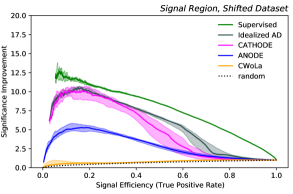
As in [39], we test this effect by introducing an artificial correlation between $x$ and $m_{JJ}$ via shifting the features $m_{J_{1}}$ and $\Delta m$ in each event according to

$$\begin{aligned} m_{J_{1}}&\rightarrow m_{J_{1}}+0.1m_{JJ}\\ \Delta m&\rightarrow\Delta m+0.1m_{JJ}\end{aligned}$$ (3)

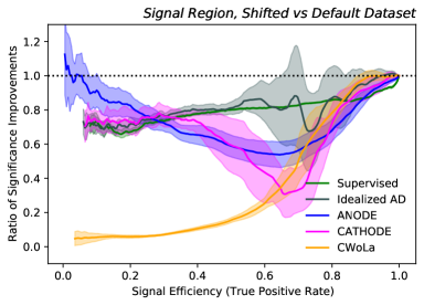
The Cathode method is applied to the shifted dataset in the otherwise same setup as described in Section III. The same benchmark methods as in Fig. 6 are tested on this shifted data analogously and compared in Fig. 8.

We see that to varying degrees, each of the different anomaly detection methods (as well as the supervised classifier) suffer from a performance loss due to the shift. In more detail:

1. Most notably, the CWoLa Hunting performance breaks down completely. This is completely expected, because the classifier can trivially deduce from the difference in $m_{JJ}$ distribution whether a data point comes from the signal region or sideband, rather than learning the desired likelihood ratio.

2. Interestingly, the performances of the idealized anomaly detector and the supervised classifier also degrade due to the shift in $x$, with the degradation somewhat larger at lower signal efficiencies. We surmise that this is due to the fact that the classifiers are trained on $x$ alone and not $m_{JJ}$; adding $m_{JJ}$ to $x$ then is effectively like smearing $x$ by another independent random variable. This in turn makes the signal less localized relative to background, which would degrade the performance of even an optimal classifier—especially at lower signal efficiencies where the classifier is benefitting most from the localization of the signal relative to the background.

3. The Anode method involves density estimation alone and not the classifier, which means that it does not have the same sensitivities to correlations that CWoLa Hunting does. However, we see from Fig. 8 (right) that there is a drop in the performance of Anode due to the shifted features, primarily at higher signal efficiencies. We attribute this to a combination of a more smeared out and difficult-to-find signal (as in the previous case), as well as worse density estimation in the presence of correlated or noisy features.

4. Finally, we come to the Cathode method. Since Cathode involves both density estimation and classification, we can think of it as a hybrid of Anode and the idealized anomaly detector. From Fig. 8 (left), we see that at lower signal efficiencies, Cathode is still comparable to the idealized anomaly detector and supervised classifier. Therefore, whatever is degrading the performances of the latter two is also affecting Cathode in a similar way. Meanwhile, at higher signal efficiencies, Cathode is noticeably worse than the idealized anomaly detector and seems to be tracking Anode instead. Here we may be seeing the additional effect of poorer density estimation as for Anode.

In appendix B, we provide further evidence that the classifiers used in Cathode and the idealized anomaly detector are suffering from smearing $x$ by the random variable $m_{JJ}$, by adding $m_{JJ}$ to the set of classifier inputs and showing that we more or less recover the lost performance that way.

IV.4 Benefits from oversampling the background model

Finally, we turn to a discussion of the benefits of oversampling events from the background model, a unique advantage of the Cathode method. For a more general discussion of the statistical properties of oversampled generative models, see Reference [98].

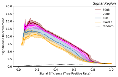
In Fig. 9 (left), we show the SIC curves for Cathode classifiers trained with different numbers of sampled background events, against a baseline Cathode classifier trained on 60,000 sampled background events. This baseline is chosen to correspond to the (fixed) number of mock data background events used in the training in the SR.

As the size of the background sample set is increased from 60,000 to 200,000, the performance improves significantly, especially at lower signal efficiencies. Increasing it further to 800,000 does not provide additional improvement, so we settled on using 200,000 sampled events in the performance plots above.

In Fig. 9 (left), we also include the CWoLa Hunting’s SIC curve for the sake of comparison. We see that even though CWoLa Hunting was trained with a comparable number (approximately 65,000) of background events in the Short Sideband region (see Appendix A.2), its performance is slightly worse than the 60,000 Cathode baseline. As discussed in Section IV.1, this is likely due to small correlations between $x$ and $m_{JJ}$ in the original LHCO R&D dataset.

Figure 9: The effect of increasing the number of sampled events when training the classifier. The total number of mock data events in the training set is fixed at 60,000 while the number of sampled events is varied. Left: For the non-shifted data, the performance is boosted by increasing the sample size to 200,000. Increasing the sample size to 800,000 does not provide any further improvement. CWoLa Hunting, which has access to approximately 65,000 background events in the data, is slightly worse than Cathode running on 60,000 samples. Right: For the correlated dataset, increasing the number of sampled events also yields a performance improvement. The solid lines are deduced from a median value of 10 fully independent trainings on the same training, validation and evaluation set. The uncertainty bands in both plots are defined the same way as in Fig. 6.

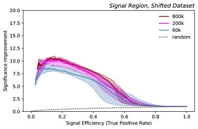
Finally, Fig. 9 (right) shows the impact of varying the sample size for Cathode when running on correlated features. Increasing the sample size here yields a modest (but significant) gain in performance.

IV.5 Background estimation

While the SIC and ROC curves represent useful metrics to assess the performance of different methods, they cannot be used in an actual particle physics experiment, since signal and background labels are not available. Instead, one must combine the anomaly score of Cathode, which achieves near-optimal signal sensitivity, with a precise method of background estimation, in order to build a complete search for new physics.

In this subsection we will present some preliminary explorations of some background estimation methods that could be combined with Cathode. A complete treatment of backgrounds, including the calculation of a calibrated $p$-value, would be well-beyond the scope of this proof-of-concept study; we leave it for future work (or for the actual experimental analyses).

Probably the most robust way to combine Cathode with background estimation would be to perform a “bump hunt” and scan several signal region bins that cover the whole $m_{jj}$ mass range. For each of the signal regions, a fit of a parametric background shape to the $m_{jj}$ distribution of events passing a cut on the anomaly score would be performed. Using this fit and its respective uncertainties, one can extract a $p$-value that reflects whether a significant excess is observed.

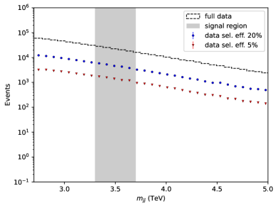
In order for Cathode to be used in such a way, it must be able to learn an unbiased estimate of the background density inside the signal region and not sculpt any features into the mass spectrum that could be accidentally found as excesses in a bump hunt. To study this, we trained Cathode again on the mock data but this time only using background events and then selected events based on the anomaly score of the model. The anomaly score for background events outside the SR is acquired by simply evaluating these events on the classifier that has been trained to learn the likelihood ratio (up to a transformation) $R(x)=p_{\mathrm{data}}(x)/p_{\mathrm{bg}}(x)$. Since the likelihood ratio only depends on the auxiliary features $x$ and not on $m_{jj}$, this model extends to events from the SBs as well. The dijet invariant mass distributions for the respective selection efficiencies of 20% and 5% can be seen in Fig. 10 (left). For reference, the full data distribution is also added. The plot clearly shows that cutting on the Cathode model score does not introduce any artificial bumps or features into the $m_{jj}$ distribution and thus it can be used in a bump hunting scenario.

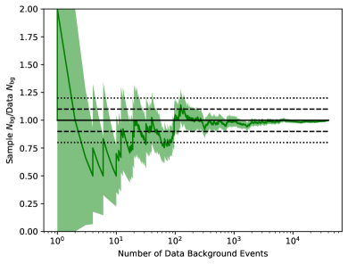
Alternatively, one could imagine another background estimation method where one uses the learned density $p_{bg}(x)$ in the SR to directly estimate the background. Versions of this approach were studied in [39] (“direct integration” and “importance sampling”), and here we present a simpler and more accurate version of this method: sampling from $p_{bg}(x)$ in the SR and measuring the background efficiency after a cut on the anomaly score. If Cathode is able to learn an unbiased estimate of the background density in the signal region, a cut on the model output should select as many artificial samples as actual background events. Fig. 10 (right) shows the ratio of the number of artificial samples and background events being selected from these cuts as a function again of the selected background events. This figure illustrates that no significant bias of the model can be observed, since the ratio is around the ideal value of 1 for almost all selection efficiencies and deviations are seen only in regions with low statistics as reflected by the error bands. Comparing with the analogous plot (Fig. 8) in [39], we see that Cathode presents a much more unbiased background estimate than Anode, especially above ${\mathcal{O}}(10^{2})$ background events. This is a reflection of the fact that the likelihood ratio learned by the Cathode classifier is much closer to unity on background events than the likelihood ratio constructed in the Anode method.

Figure 10: Investigation of background sculpting. Results for training only on background events from the mock data. Left: $m_{jj}$ distributions of background events passing a cut on the classifier output, corresponding to the indicated selection efficiencies. No significant sculpting of features into the background distribution can be observed. Right: Ratio of artificial samples and mock data background events from the signal region passing cut thresholds on the classifier output. There is no significant bias in the background density learned by the density estimator, as the number of events passing a cut on a given threshold is the same (within uncertainties) for background and artificial samples. The uncertainty bands reflect the statistical uncertainty on the number of data and artificial samples, propagated to the ratio.

V Conclusions

Cathode is a new method for anomaly detection which is model-agnostic beyond the assumption of the existence of a bump. One can think of the Cathode protocol as combining the best of the CWoLa Hunting and Anode algorithms. Similar to these two methods, we first partition data into signal region and sideband according to one feature (typically an invariant mass). As in Anode, a conditional density estimator is trained to learn the distribution of sideband data which is assumed to consist purely of background events. This density estimator is then used to generate new background-like events in the signal region. As in CWoLa Hunting, a classifier is trained to distinguish actual events in the signal region from the background-like events. However, since the background-like events are first transported via the conditional density estimator into the signal region, the result is (as opposed to the result of CWoLa Hunting) expected to be robust against correlations between features used to define the signal region ($m$) and features used to train the classifier ($x$).

As a benchmark, the LHCO R&D dataset is used to compare the different anomaly detection algorithms. We find that the Cathode method obtains near optimal performance as defined by the idealized anomaly detector. This performance is significantly better than the previous methods of CWoLa Hunting and Anode. In our test point of $S/B=0.6\%$, Cathode has a maximal SIC of 14, while CWoLa Hunting peaks at 11 and Anode at 6.5. While all anomaly detection algorithms degrade as $S/B$ decreases, Cathode is able to achieve a significance of at least $3\,\sigma$ until $S/B\approx 0.25\%$.

While only one new physics model was used to benchmark the anomaly detection methods, we expect good generalisation of CATHODE to other resonances as the construction only relies on the quality of background estimation from the sideband-regions.

We also explicitly verified that Cathode is less sensitive to correlations than other approaches. When artificially increasing the correlation between input features and the mass variable, the Cathode performance decreases to a maximum SIC of around 10 while CWoLa Hunting completely loses discrimination power. However, the artificially increased correlation entangles several issues, including potential information loss and a more difficult task for the density estimator and therefore overestimates the impact of correlation effects. The enhanced performance in the presence of correlations and the ability to oversample lead to the overall gains from Cathode relative to other methods.

Robust model-agnostic anomaly detection methods are of particular experimental interest. The improvements of Cathode over previous approaches should directly translate into more sensitive searches.

Code and Data

The code for this paper can be found at https://github.com/HEPML-AnomalyDetection/CATHODE. The LHC Olympics R&D dataset can be found at https://zenodo.org/record/4287846.

Appendix A Other methods

In this appendix, we provide more details about the implementation of the various other anomaly detection methods used in the paper. For a summary of the number of events used in each method, see Table 1.

Table 1: Numbers of events (rounded to the nearest 1,000) used for training, model selection, and evaluation for each method. All methods are evaluated on the same events.

Method	Type	Train	Validation (model selection)	Evaluation
Cathode	density estimator	500k SB data	380k SB data	340k SR background 20k SR signal
	classifier	200k SR background samples	200k SR background samples
		60k SR data	60k SR data
Anode	density estimator	500k SB data	380k SB data
		60k SR data	60k SR data
CWoLa Hunting	classifier	65k SSB data	65k SSB data
		60k SR data	60k SR data
Idealized AD	classifier	136k SR background	136k SR background
		60k SR data	60k SR data
Fully Supervised	classifier	136k SR background	136k SR background
		27k SR signal	27k SR signal

A.1 Idealized anomaly detector

We start by describing our implementation of the idealized anomaly detector, since all of the other anomaly detection approaches considered in this paper are approximations of it.

In the idealized anomaly detector, we train a classifier to distinguish the data in the SR from events taken from a perfectly simulated background model. An optimal classifier will approach the likelihood ratio

$$R_{\rm ideal}(x)={p_{\rm data}(x)\over p_{\rm bg}(x)}=f_{\rm bg}+f_{\rm sig}{p_{\rm sig}(x)\over p_{\rm bg}(x)}$$ (4)

where in the second equality we have used Eq. (2). Since this is monotonic with the signal-background likelihood ratio, events with high $R_{\rm ideal}(x)$ will also be more likely to be signal than background.

The classifier for the idealized anomaly detector was built using the same network as the Cathode classifier, using the same loss, learning rate, and optimizer. For the “data” class, we use the same training and validation split as for the other anomaly detection methods (60,000 events in the SR each for training and validation). For the “background” class, we divide up the 272,000 “simulation” background events evenly into training and validation sets.

A.2 CWoLa hunting

In the CWoLa Hunting approach [25, 26], one attempts to approximate the likelihood ratio (4) by training a classifier to distinguish the events in the SR from the events in a control region (CR) which are assumed to be all background. The network learns (a monotonic function of) the likelihood ratio given a set of observables ($x$) as:

$$R_{\rm CWoLa}(x)=\frac{p\left(x|\text{SR}\right)}{p\left(x|\text{CR}\right)}$$ (5)

Under the further assumption that the distribution of background events in the CR is the same as that of the SR, we have

$$\begin{aligned} &p(x|\text{SR})=f_{\text{sig}}p(x|\text{sig})+f_{\text{bg}}p(x|\text{bg})\\ &p(x|\text{CR})=p(x|\text{bg})\end{aligned}$$ (6)

and we approach $R_{\rm ideal}$.

To enable comparison to Cathode, we trained the CWoLa Hunting network using the same network architecture, loss, learning rate, and optimizer as the Cathode classifer. For the SR we take the same $m_{JJ}$ window as all the other methods, and analogously to previous applications on the same dataset [39], only the sidebands within 200 GeV wide strips adjacent to the SR in $m_{JJ}$ are used for the CR. We will refer to the CR for CWoLa Hunting as the Short Sideband (SSB) to distinguish this from the CR used for Anode and Cathode. This results in a total number of 130,232 background-like events before splitting them equally into training and validation sets. During training, the upper and lower SSB events are reweighted such that they contribute equally to the training and together they have the same total weight as the SR.

A.3 ANODE

The Anode approach [39] uses the same interpolated outer density estimator as Cathode for the background model. But unlike Cathode, it also trains an “inner” density estimator on the events in the SR. Then it explicitly constructs the likelihood ratio using the two separate density estimators:

$$R_{\rm ANODE}(x|m\in{\rm SR})=\frac{p_{\text{inner}}\left(x|m\in{\rm SR}\right)}{p_{\text{outer}}\left(x|m\in{\rm SR}\right)}.$$ (7)

If the density estimation and interpolation are successful, then $p_{\rm inner}=p_{\rm data}$ and $p_{\rm outer}=p_{\rm bg}$ and we again approach $R_{\rm ideal}$.

For comparison to Cathode, we trained the Anode network using the same MAF architecture as used for Cathode, with the same loss, learning rate, and optimizer as well. The split of the mock data into training and validation was 50/50 in both the SR and SB, just as in Cathode.

A.4 Supervised classifier

Finally, to understand the absolute best possible signal vs. background discrimination one could ever hope to obtain, we consider the case of labeled data and train a supervised classifier to distinguish directly between signal and background events. The supervised network used here is identical to the Cathode classifier network, including the loss, learning rate, and optimizer. We used 55,000 signal events and 272,000 background events in the SR, split equally for training and validation.

Appendix B Adding $m_{JJ}$ as a classifier input

In the main body of the paper, the approaches all use the features $x$ for data vs. background classification, but they do not use $m_{JJ}$. In this appendix, we will explore the effect of adding $m_{JJ}$ as a classifier input in Cathode, the idealized anomaly detector, and the fully supervised classifier.

Figure 11: Median significance improvement, deduced from 10 fully independent trainings on the same training, validation and evaluation set, of a supervised training (left) and the idealized anomaly detector (right) in various configurations: using the LHCO R&D dataset in its default and shifted form, both with and without $m_{JJ}$ as an additional classifier input feature. Moreover, an evaluation on an additional gaussian noise input feature to the classifier is shown for comparison.

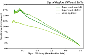
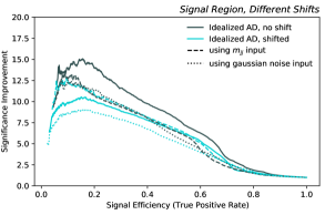
Fig. 11 (left) illustrates the effect of adding $m_{JJ}$ as an input to the fully supervised classifier trained on the unshifted and the shifted data. We see that the degradation in the fully supervised classifier performance induced by the shifted data is fully recovered by including $m_{JJ}$ as an input feature. This shows that the fully supervised classifier is able to learn to undo the shift of $x$ by $m_{JJ}$. In fact, including $m_{JJ}$ as an input even allows the fully supervised classifier to surpass its original performance, indicating that $m_{JJ}$ does have some (very mild) discriminating ability between signal and background in the signal region.

The story is a bit more complicated for the idealized anomaly detector. In Fig. 11 (right), we find that—unlike for the fully supervised classifier—adding $m_{JJ}$ as an input feature to the unshifted data actually degrades the performance of the idealized anomaly detector (dashed gray). In the signal region, the $m_{JJ}$ distributions are very similar between data and background, plus they are largely uncorrelated with the features $x$. Therefore, including $m_{JJ}$ as an input feature to the idealized anomaly detector is like including the same random noise variable with data and background. In the ideal case, one might expect the classifier can learn to shut off the random input, but in practice, given limited training data and low $S/B$, adding random noise to the anomaly detection classifier can degrade the performance. In Fig. 11 (right) we confirm the hypothesis that $m_{JJ}$ is like random noise by actually training the classifier with an additional gaussian random noise input instead of $m_{JJ}$ (gray dotted line). We find that the degradation in performance is nearly identical to training with $m_{JJ}$.

Meanwhile, the situation is quite different in the shifted case. Here $m_{JJ}$ is no longer functioning like uncorrelated random noise (since $m_{J_{1}}$ and $\Delta m$ are shifted linearly by $m_{JJ}$). Correspondingly, training with $m_{JJ}$ input does offer some benefit to the idealized anomaly detector (dashed turquoise vs. solid turquoise). Interestingly, though, it is more or less capped by the unshifted case (dashed gray). Evidently, the classifier here can learn to undo the shift in $x$, but it still cannot learn to completely shut off the input $m_{JJ}$.

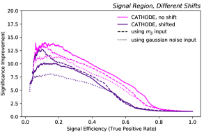
Finally, in Fig. 12 we exhibit the effects of including $m_{JJ}$ in the case of Cathode, and we see the behavior is qualitatively very similar to the idealized anomaly detector in nearly all cases. Here the effect of adding gaussian noise input to Cathode trained on the shifted data is to degrade the performance even more, whereas adding $m_{JJ}$ input improves the performance, illustrating further how $m_{JJ}$ is not just random noise for the shifted data.

In summary, we find that adding $m_{JJ}$ to the classifier inputs can have a clear benefit for anomaly detection performance when features are significantly correlated with $m_{JJ}$; however in the absence of correlations adding $m_{JJ}$ can degrade performance if it offers very little discriminating power. Clearly, the issue of feature selection for data vs. background anomaly detection is a very important and possibly delicate one, and the story is far from settled on this front.

Figure 12: Median significance improvement of CATHODE, deduced from 10 fully independent trainings on the same training, validation and evaluation set, in various configurations: using the LHCO R&D dataset in its default and shifted form, both with and without $m_{JJ}$ as an additional classifier input feature. Moreover, an evaluation on an additional gaussian noise input feature to the classifier is shown for comparison on the right.

References

- ATLAS Collaboration [2019a] ATLAS Collaboration, Exotic Physics Searches (2019a), https://twiki.cern.ch/twiki/bin/view/AtlasPublic/ExoticsPublicResults.
- ATLAS Collaboration [2019b] ATLAS Collaboration, Supersymmetry searches (2019b), https://twiki.cern.ch/twiki/bin/view/AtlasPublic/SupersymmetryPublicResults.
- ATLAS Collaboration [2019c] ATLAS Collaboration, Higgs and Diboson Searches (2019c), https://twiki.cern.ch/twiki/bin/view/AtlasPublic/HDBSPublicResults.
- CMS Collaboration [2019a] CMS Collaboration, CMS Exotica Public Physics Results (2019a), https://twiki.cern.ch/twiki/bin/view/CMSPublic/PhysicsResultsEXO.
- CMS Collaboration [2019b] CMS Collaboration, CMS Supersymmetry Physics Results (2019b), https://twiki.cern.ch/twiki/bin/view/CMSPublic/PhysicsResultsSUS.
- CMS Collaboration [2019c] CMS Collaboration, CMS Beyond-two-generations (B2G) Public Physics Results (2019c), https://twiki.cern.ch/twiki/bin/view/CMSPublic/PhysicsResultsB2G.
- LHCb Collaboration [2019] LHCb Collaboration, Publications of the QCD, Electroweak and Exotica Working Group (2019), http://lhcbproject.web.cern.ch/lhcbproject/Publications/LHCbProjectPublic/Summary_QEE.html.
- Craig et al. [2019] N. Craig, P. Draper, K. Kong, Y. Ng, and D. Whiteson, The unexplored landscape of two-body resonances, Acta Phys. Polon. B 50, 837 (2019), arXiv:1610.09392 [hep-ph] .
- Kim et al. [2020] J. H. Kim, K. Kong, B. Nachman, and D. Whiteson, The motivation and status of two-body resonance decays after the LHC Run 2 and beyond, JHEP 04, 030, arXiv:1907.06659 [hep-ph] .
- [10] B. Knuteson, A Quasi-Model-Independent Search for New High Physics at D0, ph.D. thesis, University of California at Berkeley (2000).
- Abbott et al. [2000] B. Abbott et al. (D0), Search for new physics in data at DØ using SLEUTH: A quasi model independent search strategy for new physics, Phys. Rev. D62, 092004 (2000), arXiv:hep-ex/0006011 [hep-ex] .
- Abazov et al. [2001] V. M. Abazov et al. (D0), Quasi model independent search for new physics at large transverse momentum, Phys. Rev. D64, 012004 (2001), arXiv:hep-ex/0011067 [hep-ex] .
- Abbott et al. [2001] B. Abbott et al. (D0), Quasi-model-independent search for new high physics at DØ, Phys. Rev. Lett. 86, 3712 (2001), arXiv:hep-ex/0011071 [hep-ex] .
- Aaron et al. [2009] F. D. Aaron et al. (H1), A General Search for New Phenomena at HERA, Phys. Lett. B674, 257 (2009), arXiv:0901.0507 [hep-ex] .
- Aktas et al. [2004] A. Aktas et al. (H1), A General search for new phenomena in ep scattering at HERA, Phys. Lett. B602, 14 (2004), arXiv:hep-ex/0408044 [hep-ex] .
- Cranmer [2005] K. S. Cranmer, Searching for new physics: Contributions to LEP and the LHC, Ph.D. thesis, Wisconsin U., Madison (2005).
- Aaltonen et al. [2008] T. Aaltonen et al. (CDF), Model-Independent and Quasi-Model-Independent Search for New Physics at CDF, Phys. Rev. D78, 012002 (2008), arXiv:0712.1311 [hep-ex] .
- Aaltonen et al. [2007] T. Aaltonen et al. (CDF), Model-Independent Global Search for New High-pT Physics at CDF 10.2172/922303 (2007), arXiv:0712.2534 [hep-ex] .
- Aaltonen et al. [2009] T. Aaltonen et al. (CDF), Global Search for New Physics with 2.0 fb-1 at CDF, Phys. Rev. D79, 011101 (2009), arXiv:0809.3781 [hep-ex] .
- Collaboration [2017] C. Collaboration (CMS), MUSiC, a Model Unspecific Search for New Physics, in pp Collisions at TeV, (2017).
- CMS [2011] Model Unspecific Search for New Physics in pp Collisions at sqrt(s) = 7 TeV, Tech. Rep. CMS-PAS-EXO-10-021 (CERN, Geneva, 2011).
- CMS Collaboration [2020] CMS Collaboration, MUSiC, a model unspecific search for new physics, in collisions at TeV, https://cds.cern.ch/record/2718811 (2020).
- Sirunyan et al. [2020] A. M. Sirunyan et al. (CMS), MUSiC: a model unspecific search for new physics in proton-proton collisions at 13 TeV, (2020), arXiv:2010.02984 [hep-ex] .
- D’Agnolo and Wulzer [2019] R. T. D’Agnolo and A. Wulzer, Learning New Physics from a Machine, Phys. Rev. D99, 015014 (2019), arXiv:1806.02350 [hep-ph] .
- Collins et al. [2018] J. H. Collins, K. Howe, and B. Nachman, Anomaly Detection for Resonant New Physics with Machine Learning, Phys. Rev. Lett. 121, 241803 (2018), arXiv:1805.02664 [hep-ph] .
- Collins et al. [2019] J. H. Collins, K. Howe, and B. Nachman, Extending the search for new resonances with machine learning, Phys. Rev. D99, 014038 (2019), arXiv:1902.02634 [hep-ph] .
- D’Agnolo et al. [2021] R. T. D’Agnolo, G. Grosso, M. Pierini, A. Wulzer, and M. Zanetti, Learning Multivariate New Physics, Eur. Phys. J. C 81, 89 (2021), arXiv:1912.12155 [hep-ph] .
- Farina et al. [2020] M. Farina, Y. Nakai, and D. Shih, Searching for New Physics with Deep Autoencoders, Phys. Rev. D 101, 075021 (2020), arXiv:1808.08992 [hep-ph] .
- Heimel et al. [2019] T. Heimel, G. Kasieczka, T. Plehn, and J. M. Thompson, QCD or What?, SciPost Phys. 6, 030 (2019), arXiv:1808.08979 [hep-ph] .
- Roy and Vijay [2019] T. S. Roy and A. H. Vijay, A robust anomaly finder based on autoencoders, (2019), arXiv:1903.02032 [hep-ph] .
- Cerri et al. [2019] O. Cerri, T. Q. Nguyen, M. Pierini, M. Spiropulu, and J.-R. Vlimant, Variational Autoencoders for New Physics Mining at the Large Hadron Collider, JHEP 05, 036, arXiv:1811.10276 [hep-ex] .
- Blance et al. [2019] A. Blance, M. Spannowsky, and P. Waite, Adversarially-trained autoencoders for robust unsupervised new physics searches, JHEP 10, 047, arXiv:1905.10384 [hep-ph] .
- Hajer et al. [2020] J. Hajer, Y.-Y. Li, T. Liu, and H. Wang, Novelty Detection Meets Collider Physics, Phys. Rev. D 101, 076015 (2020), arXiv:1807.10261 [hep-ph] .
- De Simone and Jacques [2019] A. De Simone and T. Jacques, Guiding New Physics Searches with Unsupervised Learning, Eur. Phys. J. C79, 289 (2019), arXiv:1807.06038 [hep-ph] .
- Mullin et al. [2021] A. Mullin, S. Nicholls, H. Pacey, M. Parker, M. White, and S. Williams, Does SUSY have friends? A new approach for LHC event analysis, JHEP 02, 160, arXiv:1912.10625 [hep-ph] .
- Casa and Menardi [2019] A. Casa and G. Menardi, Nonparametric semisupervised classification for signal detection in high energy physics, (2019), arXiv:1809.02977 [hep-ex] .
- Dillon et al. [2019] B. M. Dillon, D. A. Faroughy, and J. F. Kamenik, Uncovering latent jet substructure, Phys. Rev. D100, 056002 (2019), arXiv:1904.04200 [hep-ph] .
- Andreassen et al. [2020] A. Andreassen, B. Nachman, and D. Shih, Simulation Assisted Likelihood-free Anomaly Detection, Phys. Rev. D 101, 095004 (2020), arXiv:2001.05001 [hep-ph] .
- Nachman and Shih [2020] B. Nachman and D. Shih, Anomaly Detection with Density Estimation, Phys. Rev. D 101, 075042 (2020), arXiv:2001.04990 [hep-ph] .
- Aguilar-Saavedra et al. [2017] J. A. Aguilar-Saavedra, J. H. Collins, and R. K. Mishra, A generic anti-QCD jet tagger, JHEP 11, 163, arXiv:1709.01087 [hep-ph] .
- Crispim Romão et al. [2020] M. Crispim Romão, N. Castro, R. Pedro, and T. Vale, Transferability of Deep Learning Models in Searches for New Physics at Colliders, Phys. Rev. D 101, 035042 (2020), arXiv:1912.04220 [hep-ph] .
- Crispim Romão et al. [2021a] M. Crispim Romão, N. F. Castro, J. G. Milhano, R. Pedro, and T. Vale, Use of a generalized energy Mover’s distance in the search for rare phenomena at colliders, Eur. Phys. J. C 81, 192 (2021a), arXiv:2004.09360 [hep-ph] .
- Knapp et al. [2021] O. Knapp, O. Cerri, G. Dissertori, T. Q. Nguyen, M. Pierini, and J. R. Vlimant, Adversarially Learned Anomaly Detection on CMS Open Data: re-discovering the top quark, Eur. Phys. J. Plus 136, 236 (2021), arXiv:2005.01598 [hep-ex] .
- Dillon et al. [2020] B. M. Dillon, D. A. Faroughy, J. F. Kamenik, and M. Szewc, Learning the latent structure of collider events, JHEP 10, 206, arXiv:2005.12319 [hep-ph] .
- Crispim Romão et al. [2021b] M. Crispim Romão, N. F. Castro, and R. Pedro, Finding New Physics without learning about it: Anomaly Detection as a tool for Searches at Colliders, Eur. Phys. J. C 81, 27 (2021b), [Erratum: Eur.Phys.J.C 81, 1020 (2021)], arXiv:2006.05432 [hep-ph] .
- Amram and Suarez [2021] O. Amram and C. M. Suarez, Tag N’ Train: a technique to train improved classifiers on unlabeled data, JHEP 01, 153, arXiv:2002.12376 [hep-ph] .
- Cheng et al. [2020] T. Cheng, J.-F. Arguin, J. Leissner-Martin, J. Pilette, and T. Golling, Variational Autoencoders for Anomalous Jet Tagging, (2020), arXiv:2007.01850 [hep-ph] .
- Khosa and Sanz [2020] C. K. Khosa and V. Sanz, Anomaly Awareness, (2020), arXiv:2007.14462 [cs.LG] .
- Thaprasop et al. [2021] P. Thaprasop, K. Zhou, J. Steinheimer, and C. Herold, Unsupervised Outlier Detection in Heavy-Ion Collisions, Phys. Scripta 96, 064003 (2021), arXiv:2007.15830 [hep-ex] .
- Alexander et al. [2020] S. Alexander, S. Gleyzer, H. Parul, P. Reddy, M. W. Toomey, E. Usai, and R. Von Klar, Decoding Dark Matter Substructure without Supervision, (2020), arXiv:2008.12731 [astro-ph.CO] .
- Aguilar-Saavedra et al. [2021] J. A. Aguilar-Saavedra, F. R. Joaquim, and J. F. Seabra, Mass Unspecific Supervised Tagging (MUST) for boosted jets, JHEP 03, 012, [Erratum: JHEP 04, 133 (2021)], arXiv:2008.12792 [hep-ph] .
- Benkendorfer et al. [2021] K. Benkendorfer, L. L. Pottier, and B. Nachman, Simulation-assisted decorrelation for resonant anomaly detection, Phys. Rev. D 104, 035003 (2021), arXiv:2009.02205 [hep-ph] .
- Adrian Alan Pol and Victor Berger and Gianluca Cerminara and Cecile Germain and Maurizio Pierini [2020] Adrian Alan Pol and Victor Berger and Gianluca Cerminara and Cecile Germain and Maurizio Pierini, Anomaly Detection With Conditional Variational Autoencoders, (2020), arXiv:2010.05531 [cs.LG] .
- Mikuni and Canelli [2021] V. Mikuni and F. Canelli, Unsupervised clustering for collider physics, Phys. Rev. D 103, 092007 (2021), arXiv:2010.07106 [physics.data-an] .
- van Beekveld et al. [2021] M. van Beekveld, S. Caron, L. Hendriks, P. Jackson, A. Leinweber, S. Otten, R. Patrick, R. Ruiz De Austri, M. Santoni, and M. White, Combining outlier analysis algorithms to identify new physics at the LHC, JHEP 09, 024, arXiv:2010.07940 [hep-ph] .
- Park et al. [2020] S. E. Park, D. Rankin, S.-M. Udrescu, M. Yunus, and P. Harris, Quasi Anomalous Knowledge: Searching for new physics with embedded knowledge, JHEP 21, 030, arXiv:2011.03550 [hep-ph] .
- Faroughy [2021] D. A. Faroughy, Uncovering hidden new physics patterns in collider events using Bayesian probabilistic models, PoS ICHEP2020, 238 (2021), arXiv:2012.08579 [hep-ph] .
- Stein et al. [2020] G. Stein, U. Seljak, and B. Dai, Unsupervised in-distribution anomaly detection of new physics through conditional density estimation, (2020), arXiv:2012.11638 [cs.LG] .
- Kasieczka et al. [2021] G. Kasieczka et al., The LHC Olympics 2020 a community challenge for anomaly detection in high energy physics, Rept. Prog. Phys. 84, 124201 (2021), arXiv:2101.08320 [hep-ph] .
- Chakravarti et al. [2021] P. Chakravarti, M. Kuusela, J. Lei, and L. Wasserman, Model-Independent Detection of New Physics Signals Using Interpretable Semi-Supervised Classifier Tests, (2021), arXiv:2102.07679 [stat.AP] .
- Batson et al. [2021] J. Batson, C. G. Haaf, Y. Kahn, and D. A. Roberts, Topological Obstructions to Autoencoding, JHEP 04, 280, arXiv:2102.08380 [hep-ph] .
- Blance and Spannowsky [2020] A. Blance and M. Spannowsky, Unsupervised event classification with graphs on classical and photonic quantum computers, JHEP 21, 170, arXiv:2103.03897 [hep-ph] .
- Bortolato et al. [2021] B. Bortolato, B. M. Dillon, J. F. Kamenik, and A. Smolkovič, Bump Hunting in Latent Space, (2021), arXiv:2103.06595 [hep-ph] .
- Collins et al. [2021] J. H. Collins, P. Martín-Ramiro, B. Nachman, and D. Shih, Comparing weak- and unsupervised methods for resonant anomaly detection, Eur. Phys. J. C 81, 617 (2021), arXiv:2104.02092 [hep-ph] .
- Dillon et al. [2021] B. M. Dillon, T. Plehn, C. Sauer, and P. Sorrenson, Better Latent Spaces for Better Autoencoders, (2021), arXiv:2104.08291 [hep-ph] .
- Finke et al. [2021] T. Finke, M. Krämer, A. Morandini, A. Mück, and I. Oleksiyuk, Autoencoders for unsupervised anomaly detection in high energy physics, (2021), arXiv:2104.09051 [physics.data-an] .
- Shih et al. [2021] D. Shih, M. R. Buckley, L. Necib, and J. Tamanas, Via Machinae: Searching for stellar streams using unsupervised machine learning, Mon. Not. Roy. Astron. Soc. 509, 5992 (2021), arXiv:2104.12789 [astro-ph.GA] .
- Atkinson et al. [2021] O. Atkinson, A. Bhardwaj, C. Englert, V. S. Ngairangbam, and M. Spannowsky, Anomaly detection with Convolutional Graph Neural Networks, (2021), arXiv:2105.07988 [hep-ph] .
- Kahn et al. [2021] A. Kahn, J. Gonski, I. Ochoa, D. Williams, and G. Brooijmans, Anomalous Jet Identification via Sequence Modeling, (2021), arXiv:2105.09274 [hep-ph] .
- Aarrestad et al. [2021] T. Aarrestad et al., The Dark Machines Anomaly Score Challenge: Benchmark Data and Model Independent Event Classification for the Large Hadron Collider, (2021), arXiv:2105.14027 [hep-ph] .
- Dorigo et al. [2021] T. Dorigo, M. Fumanelli, C. Maccani, M. Mojsovska, G. C. Strong, and B. Scarpa, RanBox: Anomaly Detection in the Copula Space, (2021), arXiv:2106.05747 [physics.data-an] .
- Caron et al. [2021] S. Caron, L. Hendriks, and R. Verheyen, Rare and Different: Anomaly Scores from a combination of likelihood and out-of-distribution models to detect new physics at the LHC, (2021), arXiv:2106.10164 [hep-ph] .
- Feickert and Nachman [2021] M. Feickert and B. Nachman, A Living Review of Machine Learning for Particle Physics, (2021), arXiv:2102.02770 [hep-ph] .
- Aad et al. [2020] G. Aad et al. (ATLAS), Dijet resonance search with weak supervision using TeV collisions in the ATLAS detector, Phys. Rev. Lett. 125, 131801 (2020), arXiv:2005.02983 [hep-ex] .
- Neyman and Pearson [1933] J. Neyman and E. S. Pearson, On the problem of the most efficient tests of statistical hypotheses, Phil. Trans. R. Soc. Lond. A 231, 289 (1933).
- Metodiev et al. [2017] E. M. Metodiev, B. Nachman, and J. Thaler, Classification without labels: Learning from mixed samples in high energy physics, JHEP 10, 174, arXiv:1708.02949 [hep-ph] .
- Kasieczka et al. [2019] G. Kasieczka, B. Nachman, and D. Shih, R&D Dataset for LHC Olympics 2020 Anomaly Detection Challenge, 10.5281/zenodo.4536377 (2019).
- Sjöstrand et al. [2006] T. Sjöstrand, S. Mrenna, and P. Z. Skands, PYTHIA 6.4 Physics and Manual, JHEP 05, 026, arXiv:hep-ph/0603175 [hep-ph] .
- Sjöstrand et al. [2008] T. Sjöstrand, S. Mrenna, and P. Z. Skands, A Brief Introduction to PYTHIA 8.1, Comput. Phys. Commun. 178, 852 (2008), arXiv:0710.3820 [hep-ph] .
- de Favereau et al. [2014] J. de Favereau, C. Delaere, P. Demin, A. Giammanco, V. Lemaitre, A. Mertens, and M. Selvaggi (DELPHES 3), DELPHES 3, A modular framework for fast simulation of a generic collider experiment, JHEP 02, 057, arXiv:1307.6346 [hep-ex] .
- Mertens [2015] A. Mertens, New features in Delphes 3, Proceedings, 16th International workshop on Advanced Computing and Analysis Techniques in physics (ACAT 14): Prague, Czech Republic, September 1-5, 2014, J. Phys. Conf. Ser. 608, 012045 (2015).
- Selvaggi [2014] M. Selvaggi, DELPHES 3: A modular framework for fast-simulation of generic collider experiments, Proceedings, 15th International Workshop on Advanced Computing and Analysis Techniques in Physics Research (ACAT 2013): Beijing, China, May 16-21, 2013, J. Phys. Conf. Ser. 523, 012033 (2014).
- Cacciari et al. [2008] M. Cacciari, G. P. Salam, and G. Soyez, The anti- jet clustering algorithm, JHEP 04, 063, arXiv:0802.1189 [hep-ph] .
- Cacciari et al. [2012] M. Cacciari, G. P. Salam, and G. Soyez, FastJet User Manual, Eur. Phys. J. C72, 1896 (2012), arXiv:1111.6097 [hep-ph] .
- Cacciari and Salam [2006] M. Cacciari and G. P. Salam, Dispelling the myth for the jet-finder, Phys. Lett. B641, 57 (2006), arXiv:hep-ph/0512210 [hep-ph] .
- Thaler and Van Tilburg [2012] J. Thaler and K. Van Tilburg, Maximizing Boosted Top Identification by Minimizing N-subjettiness, JHEP 02, 093, arXiv:1108.2701 [hep-ph] .
- Thaler and Van Tilburg [2011] J. Thaler and K. Van Tilburg, Identifying Boosted Objects with N-subjettiness, JHEP 03, 015, arXiv:1011.2268 [hep-ph] .
- Papamakarios et al. [2017] G. Papamakarios, T. Pavlakou, and I. Murray, Masked Autoregressive Flow for Density Estimation, arXiv e-prints , arXiv:1705.07057 (2017), arXiv:1705.07057 [stat.ML] .
- [89] A. Hallin, J. Isaacson, G. Kasieczka, C. Krause, B. Nachman, T. Quadfasel, M. Schlaffer, D. Shih, and M. Sommerhalder, to appear, .
- Krause and Shih [2021] C. Krause and D. Shih, CaloFlow: Fast and Accurate Generation of Calorimeter Showers with Normalizing Flows, (2021), arXiv:2106.05285 [physics.ins-det] .
- Kobyzev et al. [2019] I. Kobyzev, S. J. D. Prince, and M. A. Brubaker, Normalizing Flows: An Introduction and Review of Current Methods, arXiv e-prints , arXiv:1908.09257 (2019), arXiv:1908.09257 [stat.ML] .
- Papamakarios et al. [2019] G. Papamakarios, E. Nalisnick, D. Jimenez Rezende, S. Mohamed, and B. Lakshminarayanan, Normalizing Flows for Probabilistic Modeling and Inference, arXiv e-prints , arXiv:1912.02762 (2019), arXiv:1912.02762 [stat.ML] .
- Paszke et al. [2019] A. Paszke, S. Gross, F. Massa, A. Lerer, J. Bradbury, G. Chanan, T. Killeen, Z. Lin, N. Gimelshein, L. Antiga, A. Desmaison, A. Kopf, E. Yang, Z. DeVito, M. Raison, A. Tejani, S. Chilamkurthy, B. Steiner, L. Fang, J. Bai, and S. Chintala, Pytorch: An imperative style, high-performance deep learning library, in Advances in Neural Information Processing Systems 32, edited by H. Wallach, H. Larochelle, A. Beygelzimer, F. d'Alché-Buc, E. Fox, and R. Garnett (Curran Associates, Inc., 2019) pp. 8024–8035.
- Kingma and Ba [2014] D. P. Kingma and J. Ba, Adam: A method for stochastic optimization (2014), arXiv:1412.6980 [cs.LG] .
- Lin et al. [2019] J. Lin, W. Bhimji, and B. Nachman, Machine Learning Templates for QCD Factorization in the Search for Physics Beyond the Standard Model, JHEP 05, 181, arXiv:1903.02556 [hep-ph] .
- Butter et al. [2021a] A. Butter, S. Diefenbacher, G. Kasieczka, B. Nachman, and T. Plehn, Amplifying Statistics with Ensembles of Generative Models, ICLR 2021 SimDL Workshop https://simdl.github.io/files/18.pdf (2021a).
- Pedregosa et al. [2011] F. Pedregosa, G. Varoquaux, A. Gramfort, V. Michel, B. Thirion, O. Grisel, M. Blondel, P. Prettenhofer, R. Weiss, V. Dubourg, J. Vanderplas, A. Passos, D. Cournapeau, M. Brucher, M. Perrot, and E. Duchesnay, Scikit-learn: Machine learning in Python, Journal of Machine Learning Research 12, 2825 (2011).
- Butter et al. [2021b] A. Butter, S. Diefenbacher, G. Kasieczka, B. Nachman, and T. Plehn, GANplifying event samples, SciPost Phys. 10, 139 (2021b), arXiv:2008.06545 [hep-ph] .