Conditional Extreme Value Theory for Open Set Video Domain Adaptation

Abstract.

With the advent of media streaming, video action recognition has become progressively important for various applications, yet at the high expense of requiring large-scale data labelling. To overcome the problem of expensive data labelling, domain adaptation techniques have been proposed, which transfer knowledge from fully labelled data (i.e., source domain) to unlabelled data (i.e., target domain). The majority of video domain adaptation algorithms are proposed for closed-set scenarios in which all the classes are shared among the domains. In this work, we propose an open-set video domain adaptation approach to mitigate the domain discrepancy between the source and target data, allowing the target data to contain additional classes that do not belong to the source domain. Different from previous works, which only focus on improving accuracy for shared classes, we aim to jointly enhance the alignment of the shared classes and recognition of unknown samples. Towards this goal, class-conditional extreme value theory is applied to enhance the unknown recognition. Specifically, the entropy values of target samples are modelled as generalised extreme value distributions, which allows separating unknown samples lying in the tail of the distribution. To alleviate the negative transfer issue, weights computed by the distance from the sample entropy to the threshold are leveraged in adversarial learning in the sense that confident source and target samples are aligned, and unconfident samples are pushed away. The proposed method has been thoroughly evaluated on both small-scale and large-scale cross-domain video datasets and achieved the state-of-the-art performance.

1. Introduction

With the emergence of copious streaming media data, dynamically recognising and comprehending human actions and occurrence in online videos have become progressively essential, particularly for tasks like video content recommendation (Wei et al., 2019a, b), surveillance (Ouyang et al., 2018), and video retrieval (Kwak et al., 2018). Although supervised learning techniques (Simonyan and Zisserman, 2014; Tran et al., 2015; Wang et al., 2016; Liu et al., 2017; Rahmani and Bennamoun, 2017; Yan et al., 2019) are beneficial for the tasks above, they lead to high expenses of labelling massive amounts of training data. The economical solution could be utilising a learner trained on existing labelled datasets to directly infer the labels of target datasets, yet there is often a domain shift between two datasets. Caused by the varying lighting conditions, camera angles and backgrounds, the domain shift triggers the performance drops of the learner. For example, synthetic video clips cropped from action-adventure games could be plentifully labelled and exploited, but inevitably has a huge domain shift from real-world videos such as action movie clips or sports video recordings. To address the issue of domain shift, unsupervised domain adaptation (UDA) techniques are introduced to align distributions between existing labelled data (source domain) and unlabelled data (target domain). To this end, existing UDA approaches either minimise the distribution distance across the domains (Gretton et al., 2012; Yan et al., 2017; Baktashmotlagh et al., 2013; Erfani et al., 2016; Baktashmotlagh et al., 2017) or learn the domain-invariant representations (Chen et al., 2019; Rahman et al., 2020a; Wang et al., 2021a).

In the same vein, the video-based UDA methods aim to align the features at different levels such as frame, video, or temporal relation (Chen et al., 2019; Jamal et al., 2018; Luo et al., 2020a). However, existing video-based UDA methodologies fail to address an open-set scenario when target samples come from unknown classes that are not seen during training, and can cause negative transfer across domains. Thus, the ability to recognise the unknown classes and reject them from the domain alignment pipeline is essential to the open-set unsupervised domain adaptation (OUDA) task. Moreover, the existing OUDA frameworks are mainly evaluated on still image recognition datasets which are not effective enough to identify unknown samples when applied on video recognition benchmark datasets (Zhao et al., 2019; Luo et al., 2020b; Baktashmotlagh et al., 2019; Busto and Gall, 2017; Saito et al., 2018b; Fang et al., 2019, 2021).

To overcome the above-mentioned limitations, we propose to intensify unknown recognition in open-set video domain adaptation. Our proposed framework consists of three modules. The first module is the Class-conditional Extreme Value Theory (CEVT) module that fits the entropy values of target samples to a set of generalised extreme value (GEV) distributions, where unknown samples can be efficiently identified as they lie on the tail of the distribution (Geng et al., 2018; Kotz and Nadarajah, 2000; Zhang and Patel, 2017; Oza and Patel, 2019). Samples are fitted into the multiple class-conditional GEVs depending on the model’s confidence in predicting those samples. For example, videos predicted as ”pull-up” and ”golf” are fitted into different GEVs. Then, we adaptively set a collection of thresholds for each GEV to split known and unknown samples. These fitted class-conditional GEVs with thresholds are employed in the other two modules. The second module is the class-conditional weighted domain adversarial learning pipeline to achieve the distribution alignment among shared classes and separate unknown classes. The weight of each sample is calculated by distance from entropy value to the threshold, which denotes the likelihood of belonging to the shared class or unknown class. At the inference stage, we have the third module of open-set recognition to classify samples with higher entropy than the threshold as the unknown class. This module in conjunction with class-conditional GEVs, is more robust to correctly classify hard classes than the typical approach of setting a global threshold. For example, in most of the existing OUDA approaches, the classifier predicts difficult ”push-up” samples with the highest probability as ”push-up” and with a lower probability as ”pull-up”. Subsequently, the entropy values for those samples are high, resulting in all the ”push-up” samples getting rejected by the global threshold. However, in our framework, we fit all samples predicted as ”push-up” to a GEV first, and then, we can efficiently separate ”push-up” samples and unknown samples. This framework is particularly effective for complex video sets that the model encounters more challenging training and inference due to the complex spatio-temporal composition of video features. In general, our contributions are summarised as follows:

• We propose a new Class-conditional Extreme Value Theory (CEVT) based framework for unsupervised video open-set domain adaptation that concentrates on domain-invariant representation learning via weighted domain adversarial learning.

• We investigate a new research direction of open-set video DA and introduce the CEVT model to solve the problem.

• Our proposed framework based on class-conditional extreme value theory is effective on both open-set recognition and adversarial weight generation, and it accurately recognises the unknown samples.

• We conducted extensive experiments to demonstrate the effectiveness of the proposed method on both small and large scale cross-domain video datasets and showed that the CEVT based framework achieves state-of-the-art performance. We released the source code of our proposed approach for reference: https://github.com/zhuoxiao-chen/CEVT.

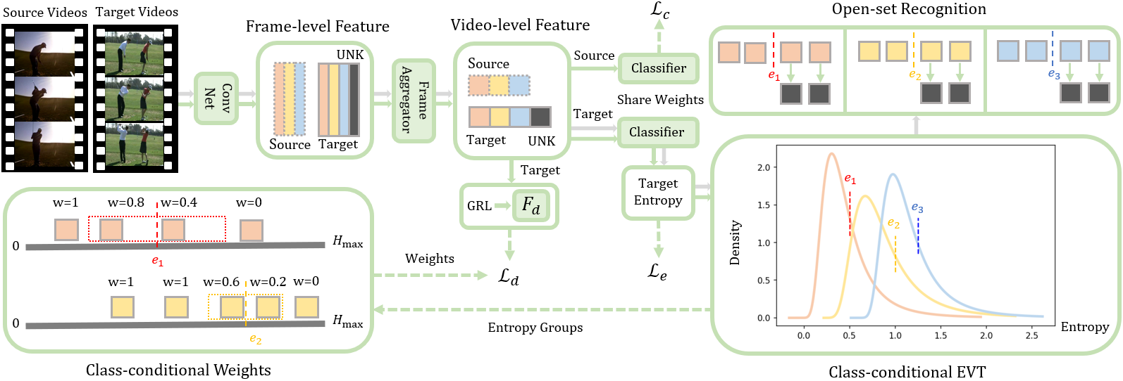
Figure 1. The overall architecture of the proposed CEVT model. Different colours indicate different classes. Class-conditional EVT in the bottom right of the figure is the probability density function (PDF) of the Generalised Extreme Value (GEV) distribution for three different entropy groups.

2. RELATED WORK

2.1. Video Action Recognition

Video action recognition is becoming increasingly important in the field of computer vision with many real-world applications, such as video surveillance (Ouyang et al., 2018), video captioning and environment monitoring (Duan et al., 2018; Krishna et al., 2017; Wang et al., 2018; Yang et al., 2017). To classify actions according to individual video frames or local motion vectors, a typical process employs a two-stream convolutional neural network (Karpathy et al., 2014; Simonyan and Zisserman, 2014). Some works utilise attention (Long et al., 2018; Ma et al., 2018), 3D convolutions (Tran et al., 2015), recurrent neural networks (Donahue et al., 2017), and temporal relation modules (Zhou et al., 2018) to better extract long-term temporal features. Another branch of work, including 3D human skeleton recognition (Liu et al., 2017; Rahmani and Bennamoun, 2017), complex object interactions (Ma et al., 2018) and pose representations (Yan et al., 2019), supplements the extracted RGB and optical flow features to alleviate the view dependency and noise caused by various lighting conditions. However, the above work necessitates costly annotations and could hardly be extended to an unseen situation, which significantly impedes the practical feasibility.

2.2. Domain Adaptation

To overcome such a limitation, Unsupervised Domain Adaptation (UDA) attempts to transfer knowledge from a labelled source domain to an unlabelled target domain. To tackle the domain shift referred to as the discrepancy of two domains, there are mainly two types of approaches. One is the discrepancy-based method that aims to minimise the distribution distance between two domains (Gretton et al., 2012; Yan et al., 2017; Baktashmotlagh et al., 2014, 2016; Rahman et al., 2019, 2020b). The other is the adversary-based method that learns the domain-invariant representation (Ganin et al., 2016; Wang et al., 2020; Moghimifar et al., 2020). In addition, adversarial generative and self-supervision-based methods are also investigated by researchers (Zhao et al., 2020). Recently, existing work has extended the UDA for harder video-based datasets. AMLS (Jamal et al., 2018) applies pre-extracted C3D (Tran et al., 2015) features to a Grassmann manifold derived from PCA and utilises adaptive kernels and adversarial learning to perform UDA. TA³N (Chen et al., 2019) attempts to simultaneously align and learn temporal dynamics with entropy-based attention. Using the topology property of the bipartite graph network, ABG (Luo et al., 2020a) explicitly models source-target interactions to learn a domain-agnostic video classifier. Nevertheless, all methods mentioned above assume that the source domain and target domain share the same label set, which is not realistic in real-world scenarios. To address such issue, OUDA that assumes the target domain contains unknown classes, has made efforts at both theoretical and experimental level (Zhao et al., 2019; Luo et al., 2020b; Baktashmotlagh et al., 2019; Busto and Gall, 2017; Bucci et al., 2020; Saito et al., 2018b). DMD (Wang et al., 2021b) attempts to perform OUDA for videos, but fails to evaluate open recognition with the appropriate metric. Despite significant progress in a broader set of video classification and OUDA, domain adaptation has received little attention for knowledge transfer across videos under the open-set setting.

3. METHODOLOGY

In this section, we first give a formal definition of the Open-set Unsupervised Video Domain Adaptation (OUVDA), and then go through the details of our proposed CEVT framework, illustrated in Figure 1.

3.1. Problem Formulation

We are given a labelled source video set $\mathcal{S}=\{(X_{i}^{s},y_{i})\}_{i=1}^{N_{s}}\sim\mathbb{P}^{s}$ and an unlabelled target video collection $\mathcal{T}=\{(X_{j}^{t})\}_{j=1}^{N_{t}}\sim\mathbb{Q}^{t}$, where $N_{s}$ and $N_{t}$ are the number of videos in each domain, respectively. Video samples in the source domain $\mathcal{S}$ and the target domain $\mathcal{T}$ are drawn from different probability distributions, i.e., $\mathbb{P}^{s}\neq\mathbb{Q}^{t}$. The two domains share $C$ common classes as the known classes. There is the additional class in the target domain $\mathcal{T}$ not shared with the source domain $\mathcal{S}$, which is regarded as the $C+1$, i.e., the unknown class. Each source video $X_{i}^{s}$ or target video $X_{j}^{t}$ is composed of $K$ frames, i.e., $X_{i}^{s}={\{x_{ik}^{s}\}}_{k=1}^{K}$ and $X_{j}^{t}={\{x_{jk}^{t}\}}_{k=1}^{K}$, where $x_{ik}^{s},x_{jk}^{t}\in\mathbb{R}^{D}$ represent the $D$ dimensional feature vector of k-th frame in i-th source video and j-th target video, respectively. The primary goal of our method is to learn a classifier: $F_{\mathcal{T}}(\cdot;\theta_{c})$ for predicting the $C$ labels of unlabelled videos in target domain and a collection of functions $F_{GEV}(\cdot;\mu,\sigma,\xi)$ to recognise samples from the unknown class $C+1$ in target domain.

3.2. Source Classification

We first feed both source videos and target videos into ResNet (He et al., 2015) to obtain the frame-level features, i.e., $\{{\{x_{ik}^{s}\}}_{k=1}^{K}\}_{i=1}^{N_{s}}$ and $\{{\{x_{jk}^{t}\}}_{k=1}^{K}\}_{j=1}^{N_{t}}$ for source and target domain, respectively. Then the frame-level features are transformed into video-level features, i.e., $\{V_{i}^{s}\}_{i=1}^{N_{s}}$ and $\{V_{j}^{t}\}_{j=1}^{N_{t}}$ by frame aggregation techniques, with $V_{i}^{s},V_{i}^{t}\in\mathbb{R}^{D}$. Without loss of generality, we utilise the mean Average Pooling (AvgPool), which is to produce a unified video representation by temporal averaging of the frame features. Thus, each source video-level feature $V_{i}^{s}$ and target video-level feature $V_{j}^{t}$ are defined as below:

(1) $$V_{i}^{s}=\frac{1}{K}\sum_{k=1}^{K}x_{ik}^{s},V_{j}^{t}=\frac{1}{K}\sum_{k=1}^{K}x_{jk}^{t}.$$

Next, the aggregated features with labels $\{(V_{i}^{s},y_{i})\}_{i=1}^{N_{s}}$ from the source domain are fed into the source classifier $F_{\mathcal{S}}(\cdot;\theta_{c})$, which is trained to minimise the cross entropy loss,

(2) $$\mathcal{L}_{c}=-\mathbb{E}_{(V,y)\sim\mathbb{P}^{s}}[\text{log}F_{\mathcal{S}}(V)].$$

The parameters of the source classifier $F_{\mathcal{S}}(\cdot;\theta_{c})$ are shared with the target classifier $F_{\mathcal{T}}(\cdot;\theta_{c})$, which is used to predict $C$ classes for target samples. Figure 1 shows the entire source classification process by a green array that starts from the videos on the left to the classification loss $\mathcal{L}_{c}$.

3.3. Entropy-based Weights for Domain Adversarial Learning

To align the distributions of the video-level source and target features, we propose a novel class-conditional EVT to generate conditional weights for domain adversarial learning by fitting the entropy values of target samples. The weighted domain adversarial learning can effectively align the known samples from both domains and separate the unknown samples from the target domain simultaneously by assigning instance-level weight to each sample. The samples which come by high probability from known classes are assigned a large weight. Conversely, samples that are likely to be unknown are given a small weight. Finally, all the features are multiplied by their weights and fed into the standard domain adversarial learning module $F_{d}(\cdot;\theta_{d})$ with the Gradient Reversal Layer (GRL), as shown in Figure 1.

Class-conditional Extreme Value Theory. To obtain the weight for each sample, we feed target samples $\{(V_{j}^{t})\}_{j=1}^{N_{t}}$ into target classifier $F_{\mathcal{T}}(\cdot;\theta_{c})$ to get the predictions for shared $C$ classes. Then, the entropy value of each target sample can be computed from its prediction,

(3) $$H(V^{t})=-\sum_{c=1}^{C}F_{\mathcal{T}}(V^{t})_{c}\text{log}F_{\mathcal{T}}(V^{t})_{c},$$

where $F_{\mathcal{T}}(\cdot;\theta_{c})_{c}$ denotes the prediction of class $c$ by the classifier. Then, the entropy values of target samples are partitioned into $C$ entropy groups, i.e., $G=\{G_{i}\}_{i=1}^{C}$. Target samples predicted to be from $i$-th class are allocated to the group $G_{i}$. The set of class-conditional entropy group is formulated as:

(4) $$G=\{H(V^{t}):\text{argmax}(F_{\mathcal{T}}(V^{t}))=i\}_{i=1}^{C}.$$

Next, each group is fitted into a GEV distribution to obtain a set of CDFs of GEV, i.e., $\{F_{GEV}(\cdot\mid\text{class}=i)\}_{i=1}^{C}$, where $F_{GEV}(\cdot\mid\text{class}=i)$ indicates the CDF function fitted by entropy values in $i$-th group $G_{i}$. The CDF of GEV is calculated as,

(5) $$F_{GEV}(x;\mu,\sigma,\xi)=\text{exp}(-(1+\xi(\frac{x-\mu}{\sigma}))^{-\frac{1}{\xi}}),$$

where $\mu$, $\sigma$, and $\xi$ are three parameters of GEV, determined by fitting data. Utilising the class-conditional EVT can complement the lack of class information for entropy.

Class-conditional Weights. After fitting GEVs using entropy values of each entropy group, we set a global threshold $\delta$ for all the CDFs in $\{F_{GEV}(\cdot\mid\text{class}=i)\}_{i=1}^{C}$. Then, a set of class-conditional entropy threshold is computed for each group, denoted as,

(6) $$\{e_{i}:F_{GEV}(e_{i}\mid\text{class}=i)=\delta\}_{i=1}^{C}.$$

Given the target sample, $V^{t}$ is classified in $i$-th class, if $H(V^{t})$ is much greater or smaller than $e_{i}$, meaning this sample is very likely to be known or unknown. Then, we assign the weight as 1 or 0 to $V^{t}$. If the $H(V^{t})$ is close to $e_{i}$, meaning the classifier is unsure about $H(V^{t})$, we assign it a weight which linearly depends on distance from its entropy value to the corresponding class conditional entropy threshold $e_{i}$. The interval for linear variation of weight is named as mixture entropy interval, where most knowns or unknowns are mixed within this interval. The class-conditional weight can be formulated as,

(7) $$W(V^{t}\mid\text{class}=i)=0.5+\frac{e_{i}-H(V^{t})}{\text{min}(e_{i},(H_{max}(C)-e_{i}))},$$

(8) $$W(V^{t}\mid\text{class}=i)=\text{min}(1,\text{max}(0,W(V^{t}))),$$

where $H_{max}(C)$ is the entropy value of the evenly spaced vector with norm $|C|$, with each element of the vector being $1/C$. Two black line segments shown in the left bottom of Figure 1 shows the total entropy interval $[0,H_{max}]$, on which all the entropy values lie. The mixture entropy interval is $[e_{i}-\frac{\text{min}(e_{i},(H_{max}(C)-e_{i})}{2},e_{i}+\frac{\text{min}(e_{i},(H_{max}(C)-e_{i})}{2}]$, demonstrated by the dashed rectangles. The length of the entropy mixture interval varies depending on the distance from $e_{i}$ to either 0 or $H_{max}$, shown by red and yellow dashed rectangles of different length. The entropy threshold $e_{i}$ that is close to either 0 or $H_{max}$ indicates if the $i$-th class is easy or hard, and the distribution of class group $G_{i}$ has small variance. Thus, we need a small mixture for those dense group of entropy values to smoothly assign the weights.

Weighted Domain Adversarial Learning. After obtaining weights for all the target samples by the class-conditional EVT technique, we train the domain classifier on the target video features multiplied with instance-level weights. The weighted domain classification loss is calculated by,

(9) $$\begin{split}\mathcal{L}_{d}&=\mathbb{E}_{V\sim\mathbb{P}^{s}}[\text{log}F_{d}(V)]\\ &+\mathbb{E}_{V\sim\mathbb{Q}^{t}}[W(V\mid\text{class}=\text{argmax}(F_{\mathcal{T}}(V))\times\text{log}(1-F_{d}(V))].\end{split}$$

Gradually, with the proposed conditional EVT and weighted domain adversarial learning modules, known samples of both domains are aligned, and unknown samples of the target domain get separated from known samples.

3.4. Entropy Maximisation

To further separate the unknown samples, we utilise entropy maximum loss to progressively increase the entropy values of the overall target samples, defined as,

(10) $$\mathcal{L}_{e} =-\mathbb{E}_{V\sim\mathbb{Q}^{t}}[-\sum_{c=1}^{C}F_{\mathcal{T}}(V)_{c}\text{log}F_{\mathcal{T}}(V)_{c}].$$

With the weighted domain adversarial learning, known target samples become similar to source samples. The entropy values of source samples gradually decreases because the source classifier is fully trained to optimise the cross-entropy loss $\mathcal{L}_{c}$. Thus, in the target domain, the entropy values of known samples decrease as well when optimising the two losses of $\mathcal{L}_{c}$ and $\mathcal{L}_{d}$, while the entropy values of unknown samples increase when optimising $\mathcal{L}_{e}$ loss. Eventually, the unknown samples are optimally separated from known samples.

Table 1. Performance comparisons on the UCF→HMDB.

Methods	ALL	OS	OS*	UNK	HOS
DANN (Ganin et al., 2016) + OSVM (Jain et al., 2014)	66.11	53.41	48.33	83.89	61.33
JAN (Long et al., 2017) + OSVM (Jain et al., 2014)	61.11	51.59	47.78	74.44	58.20
AdaBN (Li et al., 2018) + OSVM (Jain et al., 2014)	60.65	61.35	61.67	59.44	60.54
MCD (Saito et al., 2018a) + OSVM (Jain et al., 2014)	66.67	60.32	57.78	75.56	65.48
TA2N (Chen et al., 2019) + OSVM (Jain et al., 2014)	65.28	58.73	56.11	74.44	63.99
TA3N (Chen et al., 2019) + OSVM (Jain et al., 2014)	62.25	55.95	53.33	71.67	61.16
OSBP (Saito et al., 2018b) + AvgPool	67.19	55.64	50.83	84.47	63.47
Ours	75.28	61.59	56.11	94.44	70.40

Table 2. Performance comparisons on the HMDB→UCF.

Methods	ALL	OS	OS*	UNK	HOS
DANN (Ganin et al., 2016) + OSVM (Jain et al., 2014)	64.62	64.61	62.94	74.67	68.31
JAN (Long et al., 2017) + OSVM (Jain et al., 2014)	61.47	64.47	62.91	73.80	67.92
AdaBN (Li et al., 2018) + OSVM (Jain et al., 2014)	62.87	60.86	58.78	73.36	65.27
MCD (Saito et al., 2018a) + OSVM (Jain et al., 2014)	66.73	64.96	63.48	73.80	68.25
TA2N (Chen et al., 2019) + OSVM (Jain et al., 2014)	63.40	63.88	61.35	79.04	69.08
TA3N (Chen et al., 2019) + OSVM (Jain et al., 2014)	60.60	61.84	58.39	82.53	68.39
OSBP (Saito et al., 2018b) + AvgPool	64.84	59.61	55.26	85.71	67.19
Ours	70.58	69.29	66.79	84.28	74.52

3.5. Optimisation

The ultimate objective is to learn the optimal parameters for the CEVT model,

(11) $$\begin{split}&(\theta_{c}^{*},\theta_{e}^{*})=\text{argmin}\>\mathcal{L}_{c}+\beta\mathcal{L}_{e}-\gamma\mathcal{L}_{d},\\ &(\theta_{d}^{*})=\text{argmin}\>\mathcal{L}_{c}+\beta\mathcal{L}_{e}+\gamma\mathcal{L}_{d},\end{split}$$

with $\beta$ and $\gamma$ the coefficients of the entropy maximisation loss and weighted adversarial loss, respectively.

3.6. Inference

In this section, we explain the inference stage of the proposed CEVT after the model parameters are optimised. The inference process is denoted by grey arrays shown in Figure 1. The target videos are fed into the convolution network, frame aggregator, and the target classifier $F_{\mathcal{T}}(\cdot;\theta_{c}^{*})$. Then, the predictions are passed into the class-conditional EVT module for open-set recognition. The predicted class $y\in|C+1|$ of each input target videos is represented as,

(12) $$\begin{split}&y=F_{\mathcal{T}}(V^{t})\\ &y=C+1\>\>\text{if}\;F_{GEV}(V_{t}\mid\text{class}=\text{argmax}(F_{\mathcal{T}}(V^{t})))>\delta.\end{split}$$

4. EXPERIMENTS

In this section, we empirically evaluate the performance of the proposed CEVT model on two datasets, UCF-HMDB and UCF-Olympic for unsupervised open-set domain adaptation.

4.1. Datasets

The UCF-HMDB is the intersected subset covering 12 highly relevant categories of two large-scale video action datasets, the UCF101 (Soomro et al., 2012) and HMDB51 (Kuehne et al., 2011), including Climb, Fencing, Golf, Kick Ball, pull-up, Punch, push-up, Ride Bike, Ride Horse, Shoot Ball, Shoot Bow and Walk. The UCF-Olympic have six common categories from the UCF101 and Olympic Sports Dataset (Niebles et al., 2010), which involves Basketball, Clearn and Jerk, Diving, Pole Vault, Tennis and Discus Throw. These dataset partitioning strategies follow (Chen et al., 2019) to make a fair comparison. Likewise, we utilise the pre-extracted frame-level features by ResNet101 model pre-trained on ImageNet. In terms of known/unknown category splitting, we select the first half categories as known classes, and all the remaining categories are labelled as unknown, for both UCF-HMDB and UCF-Olympic.

4.2. Evaluation Metrics

To compare the performance of the proposed CEVT and the baseline methods, we adopt four widely used metrics (Bucci et al., 2020)(Saito et al., 2018b) for evaluating OUDA tasks. The accuracy (ALL) is the correctly predicted target samples over all target samples. OS is the average class accuracy over the classes. OS* is the average class accuracy over the known classes. UNK is the unknown class accuracy. HOS is the harmonic mean of OS* and UNK formulated as: $2\times\frac{\textbf{OS}^{*}\times\textbf{UNK}}{\textbf{OS}^{*}+\textbf{UNK}}$ . HOS is the most meaningful metric for evaluating OUDA tasks because it can best reflect the balance between OS* and UNK.

4.3. Baselines

We compare our proposed CEVT with three types of state-of-the-art domain adaptation methods: the close-set method for images, the close-set method for videos and the open-set method for images. The close-set domain adaptation methods for images are extended to align the distributions of aggregated frames from source and target domains, which include Domain-Adversarial Neural Network (DANN) (Ganin et al., 2016), Joint Adaptation Network (JAN) (Long et al., 2017), Adaptive Batch Normalisation (AdaBN) (Li et al., 2018) and Maximum Classier Discrepancy (MCD) (Saito et al., 2018a). In terms of the close-set approach for videos, Temporal Attentive Adversarial Adaptation Network (TA²N) (Chen et al., 2019) and Temporal Adversarial Adaptation Network (TA³N) (Chen et al., 2019) are adopted for comparison. We equip the above open-set methods with the OSVM (Jain et al., 2014) for open recognition. As for the open-set method for images, OUDA by Backpropagation (OSBP) (Saito et al., 2018b) extended by frame aggregator is made into comparison.

4.4. Implementation Details

All the baselines and our approach are implemented by PyTorch (Paszke et al., 2019) on one server with two GeForce GTX 2080 Ti GPUs. We follow (Chen et al., 2019) to sample a specified number of frames with uniform spacing from each video for training and extract a 2048-D feature vector from each frame by the Resnet-101 pre-trained on ImageNet. To ensure a fair comparison, we fix $K$ to 16 for all methods using average pooling, and follow the optimisation strategy in (Chen et al., 2019) to utilise the stochastic gradient descent (SGD) as the optimiser, and learning-rate-decreasing techniques from DANN (Ganin et al., 2016), with learning rate, momentum, and weight decay of 0.03, 0.9 and $1\times 10^{-4}$, respectively. The scale of datasets determines the size of the source batch, 32 for UCF-Olympic and 128 for UCF-HMDB. The size of the target batch is computed by multiplying the source batch with the ratio between the source and target datasets. The loss coefficient $\beta$ is set as 1, 10, 0.19, 0.22, and $\gamma$ is set as 0.9, 0.7, 1.83, 5, for UCF→HMDB, HMDB→UCF, UCF→Olympic and Olympic→UCF, respectively. The EVT threshold is set as 0.4, 0.45, 0.6 and 0.29 for the above tasks, respectively.

Table 3. Performance comparisons on the Olympic→UCF.

Methods	ALL	OS	OS*	UNK	HOS
DANN (Ganin et al., 2016) + OSVM (Jain et al., 2014)	83.33	84.93	86.38	80.60	83.39
JAN (Long et al., 2017) + OSVM (Jain et al., 2014)	88.75	84.23	80.46	95.52	87.35
AdaBN (Li et al., 2018) + OSVM (Jain et al., 2014)	84.17	80.09	76.93	89.55	82.76
MCD (Saito et al., 2018a) + OSVM (Jain et al., 2014)	83.75	84.65	85.50	82.09	83.76
TA2N (Chen et al., 2019) + OSVM (Jain et al., 2014)	87.92	82.74	78.48	95.52	86.17
TA3N (Chen et al., 2019) + OSVM (Jain et al., 2014)	85.83	85.64	85.58	85.82	85.70
OSBP (Saito et al., 2018b) + AvgPool	89.06	86.23	84.31	92.00	87.98
Ours	89.17	87.54	86.38	91.04	88.65

Table 4. Performance comparisons on the UCF→Olympic.

Methods	ALL	OS	OS*	UNK	HOS
DANN (Ganin et al., 2016) + OSVM (Jain et al., 2014)	94.44	95.33	96.67	91.30	93.91
JAN (Long et al., 2017) + OSVM (Jain et al., 2014)	94.44	96.74	100.00	86.96	93.02
AdaBN (Li et al., 2018) + OSVM (Jain et al., 2014)	87.04	83.86	78.48	100.00	87.95
MCD (Saito et al., 2018a) + OSVM (Jain et al., 2014)	87.04	86.74	86.67	86.96	86.81
TA2N (Chen et al., 2019) + OSVM (Jain et al., 2014)	96.30	97.83	100.00	91.30	95.45
TA3N (Chen et al., 2019) + OSVM (Jain et al., 2014)	88.89	88.74	87.88	91.03	89.56
OSBP (Saito et al., 2018b) + AvgPool	96.88	95.83	94.44	100.00	97.14
Ours	98.15	97.73	96.97	100.00	98.46

4.5. Comparisons with State-of-The-Art

We clearly report the performance of the proposed CEVT and baseline methods on UCF-HMDB and UCF-Olympic as shown in Table 1, Table 2, Table 3 and Table 4. The proposed CEVT model outperforms all the compared state-of-the-art domain adaptation approaches, improving the HOS by 4.92%, 5.44%, 1.32% and 0.67% on the adaptation task UCF→HMDB, HMDB→UCF, UCF→Olympic and Olympic→UCF, respectively. It is worth noting that the proposed model achieves significant performance boosts for the larger-scale datasets of UCF-Olympic. Also, note that the outstanding performance gain of the proposed framework for the most challenging transfer task, i.e., UCF→HMDB, illustrates the better adaptation ability of our approach. Some methods achieve 100% on OS* or UNK for the UCF→Olympic task because this task is relatively easier than other tasks, and the validation set has limited samples. Also, there is usually a trade-off between these two metrics. For example, JAN achieves 100% on OS* but gets the lowest score (86.95%) on UNK. Conversely, AdaBn achieves 100% on UNK but has the worst performance (78.48%) on OS*. The proposed CEVT is superior to all baselines, as it achieves remarkably high OS* and UNK simultaneously.

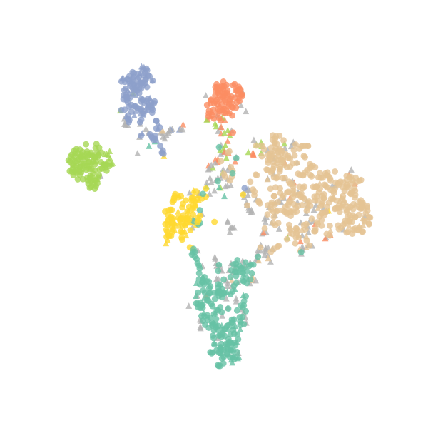
(a) DANN + OSVM

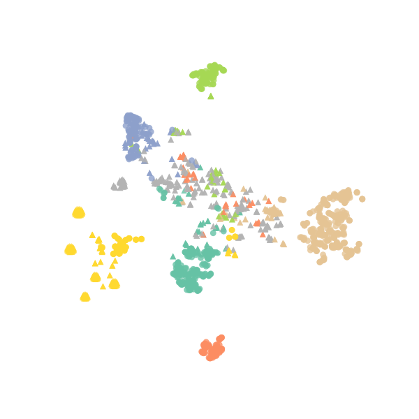
(b) OSBP + AvgPool

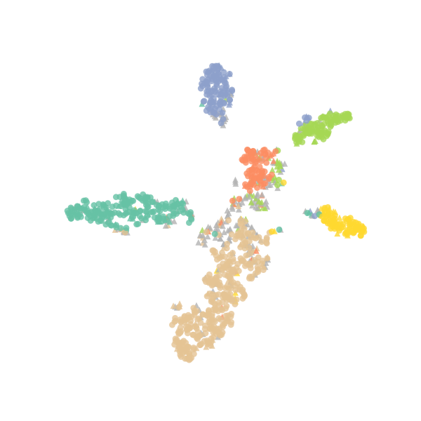
(c) TA³N + OSVM

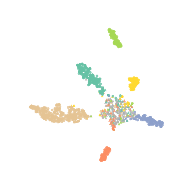
(d) Ours

Figure 2. The t-SNE visualisation of the learned source and target video representations on the UCF→HMDB task.

Table 5. The ablation performance (HOS%) of the proposed CEVT model on the UCF-HMDB dataset. ”w” indicates with and ”w/o” indicates without.

Methods	UCF→HMDB	HMDB→UCF
CEVT w/o $\mathcal{L}_{e}$ & $\mathcal{L}_{d}$	62.09	71.42
CEVT w/o $\mathcal{L}_{e}$	64.04	72.01
CEVT w/o $\mathcal{L}_{d}$	67.41	72.88
CEVT w unweighted $\mathcal{L}_{d}$	68.03	72.56
CEVT	70.40	74.52

4.6. Ablation Study

We use the UCF-HMDB dataset to investigate the performance of the proposed modules of the model CEVT. Table 5 summarises the experimental results among methods with different removed functions. Removing both weighted domain adversarial learning and entropy maximisation learning, the performance of CEVT w/o $\mathcal{L}_{e}$ drop (8.31%) significantly when adapting from UCF to HMDB compared with the complete model. Although there is only source classification and EVT method for unknown recognition left, the dropped performance (62.09% and 71.42%) is still better than most of the baseline methods equipped with OSVM, proving the robustness of EVT in terms of unknown recognition tasks. The CEVT w/o $\mathcal{L}_{e}$ refers to the variant without the entropy maximisation loss, which causes HOS drop (6.36% and 1.09% ) in both adaptation directions. Removing the weighted adversarial learning, referred to as CEVT w/o $\mathcal{L}_{d}$, result in a performance decrease slightly in either direction. The CEVT w unweighted $\mathcal{L}_{d}$ indicates that the weights of all instances are set as 1 for $\mathcal{L}_{d}$, which performs worse than weighted $\mathcal{L}_{d}$. The transfer task from UCF to HMDB is more challenging than the opposite direction. Thus, the proposed modules are more capable of handling challenging adaptation tasks.

4.7. Parameter Sensitivity

To explore the sensitivity of the loss coefficients of the proposed CEVT, we run the experiments on the dataset UCF-HMDB with changing values of $\beta$ and $\gamma$, which are used to adjust the weighted adversarial loss and the entropy maximisation loss, respectively. Even though both $\beta$ and $\gamma$ vary in a wide interval, as plotted in Figure 3, the average HOS of the proposed CEVT is very steady for both UCF→HMDB and HMDB→UCF tasks. No matter how the coefficients $\beta$ varies, the fluctuation range of HOS does not exceed $3\%$. As for the $\gamma$, the fluctuation range is less than $1.5\%$. This demonstrates the resistance of our methodology to varying loss coefficients.

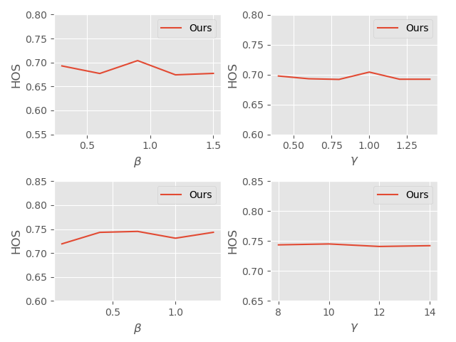
Figure 3. Performance (HOS) comparisons of the proposed CEVT with respect to the varying loss coefficients on the UCF→HMDB (shown in the upper row) and HMDB→UCF (shown in the bottom row) adaptation tasks.

4.8. Visualisation

To intuitively show how our model closes the domain shift between source and target domains as well as effectively recognises the unknown samples, we apply the t-SNE (van der Maaten and Hinton, 2008) to visualise the extracted features from baseline models, DANN, OSPB, TA³N and our proposed CEVT on the UCF→HMDB task as shown in Figure 2. Different colours denote different classes, and unknown samples are grey. The source videos are represented by circles, while triangles represent the target videos. Compared to the baseline methods, it is noticeable that the features extracted by CEVT produce tighter clusters, and unknown samples are better clustered to the centre.

5. CONCLUSION

In this work, we propose a CEVT framework to tackle the problem of open-set unsupervised video domain adaptation. Unlike previous works, we intensify the open recognition to jointly improve the accuracy of the both known and unknown classes. Experiments demonstrate that the proposed algorithm outperforms state-of-the-art methods on both large and small video datasets. Future work includes testing CEVT for still images, and equipping the proposed CEVT with other frame aggregators for videos.

References

- (1)
- Baktashmotlagh et al. (2019) Mahsa Baktashmotlagh, Masoud Faraki, Tom Drummond, and Mathieu Salzmann. 2019. Learning Factorized Representations for Open-Set Domain Adaptation. In Proc. International Conference on Learning Representations, ICLR 2019.
- Baktashmotlagh et al. (2013) Mahsa Baktashmotlagh, Mehrtash Tafazzoli Harandi, Brian C. Lovell, and Mathieu Salzmann. 2013. Unsupervised Domain Adaptation by Domain Invariant Projection. In Proc. International Conference on Computer Vision, ICCV 2013. IEEE Computer Society, 769–776.
- Baktashmotlagh et al. (2014) Mahsa Baktashmotlagh, Mehrtash Tafazzoli Harandi, Brian C. Lovell, and Mathieu Salzmann. 2014. Domain Adaptation on the Statistical Manifold. In Proc. Conference on Computer Vision and Pattern Recognition, CVPR 2014. 2481–2488.
- Baktashmotlagh et al. (2016) Mahsa Baktashmotlagh, Mehrtash Tafazzoli Harandi, and Mathieu Salzmann. 2016. Distribution-Matching Embedding for Visual Domain Adaptation. Journal of Machine Learning Research 17 (2016), 108:1–108:30.
- Baktashmotlagh et al. (2017) Mahsa Baktashmotlagh, Mehrtash Tafazzoli Harandi, and Mathieu Salzmann. 2017. Learning Domain Invariant Embeddings by Matching Distributions. In Domain Adaptation in Computer Vision Applications. 95–114.
- Bucci et al. (2020) Silvia Bucci, Mohammad Reza Loghmani, and Tatiana Tommasi. 2020. On the Effectiveness of Image Rotation for Open Set Domain Adaptation. In Proc. European Conference on Computer Vision, ECCV 2020. 422–438.
- Busto and Gall (2017) Pau Panareda Busto and Juergen Gall. 2017. Open Set Domain Adaptation. In Proc. International Conference on Computer Vision, ICCV 2017. 754–763.
- Chen et al. (2019) Min-Hung Chen, Zsolt Kira, Ghassan Alregib, Jaekwon Yoo, Ruxin Chen, and Jian Zheng. 2019. Temporal Attentive Alignment for Large-Scale Video Domain Adaptation. In Proc. International Conference on Computer Vision, ICCV 2019. 6320–6329.
- Donahue et al. (2017) Jeff Donahue, Lisa Anne Hendricks, Marcus Rohrbach, Subhashini Venugopalan, Sergio Guadarrama, Kate Saenko, and Trevor Darrell. 2017. Long-Term Recurrent Convolutional Networks for Visual Recognition and Description. IEEE Transactions on Pattern Analysis and Machine Intelligence 39, 4 (2017), 677–691.
- Duan et al. (2018) Xuguang Duan, Wen-bing Huang, Chuang Gan, Jingdong Wang, Wenwu Zhu, and Junzhou Huang. 2018. Weakly Supervised Dense Event Captioning in Videos. In Proc. Conference on Neural Information Processing Systems, NeurIPS 2018. 3063–3073.
- Erfani et al. (2016) Sarah M. Erfani, Mahsa Baktashmotlagh, Masud Moshtaghi, Vinh Nguyen, Christopher Leckie, James Bailey, and Kotagiri Ramamohanarao. 2016. Robust Domain Generalisation by Enforcing Distribution Invariance. In Proc. International Joint Conference on Artificial Intelligence, IJCAI 2016. 1455–1461.
- Fang et al. (2021) Zhen Fang, Jie Lu, Anjin Liu, Feng Liu, and Guangquan Zhang. 2021. Learning Bounds for Open-Set Learning. In Proc. of the 37th International Conference on Machine Learning, ICML 2021. 3122–3132.
- Fang et al. (2019) Zhen Fang, Jie Lu, Feng Liu, Junyu Xuan, and Guangquan Zhang. 2019. Open Set Domain Adaptation: Theoretical Bound and Algorithm. IEEE Transactions on Neural Networks and Learning Systems (2019).
- Ganin et al. (2016) Yaroslav Ganin, Evgeniya Ustinova, Hana Ajakan, Pascal Germain, Hugo Larochelle, François Laviolette, Mario Marchand, and Victor S. Lempitsky. 2016. Domain-Adversarial Training of Neural Networks. Journal of Machine Learning Research 17 (2016), 59:1–59:35.
- Geng et al. (2018) Chuanxing Geng, Sheng-Jun Huang, and Songcan Chen. 2018. Recent Advances in Open Set Recognition: A Survey. CoRR abs/1811.08581 (2018).
- Gretton et al. (2012) Arthur Gretton, Karsten M. Borgwardt, Malte J. Rasch, Bernhard Schölkopf, and Alexander J. Smola. 2012. A Kernel Two-Sample Test. Journal of Machine Learning Research 13 (2012), 723–773.
- He et al. (2015) Kaiming He, Xiangyu Zhang, Shaoqing Ren, and Jian Sun. 2015. Deep Residual Learning for Image Recognition. CoRR abs/1512.03385 (2015).
- Jain et al. (2014) Lalit P. Jain, Walter J. Scheirer, and Terrance E. Boult. 2014. Multi-class Open Set Recognition Using Probability of Inclusion. In Proc. European Conference on Computer Vision, ECCV 2014. 393–409.
- Jamal et al. (2018) Arshad Jamal, Vinay P. Namboodiri, Dipti Deodhare, and K. S. Venkatesh. 2018. Deep Domain Adaptation in Action Space. In Proc. British Machine Vision Conference, BMVC 2018. 264.
- Karpathy et al. (2014) Andrej Karpathy, George Toderici, Sanketh Shetty, Thomas Leung, Rahul Sukthankar, and Fei-Fei Li. 2014. Large-Scale Video Classification with Convolutional Neural Networks. In Proc. Conference on Computer Vision and Pattern Recognition, CVPR 2014. 1725–1732.
- Kotz and Nadarajah (2000) Samuel Kotz and Saralees Nadarajah. 2000. Extreme value distributions: theory and applications. World Scientific.
- Krishna et al. (2017) Ranjay Krishna, Kenji Hata, Frederic Ren, Li Fei-Fei, and Juan Carlos Niebles. 2017. Dense-Captioning Events in Videos. In Proc. International Conference on Computer Vision, ICCV 2017. 706–715.
- Kuehne et al. (2011) Hildegard Kuehne, Hueihan Jhuang, Estíbaliz Garrote, Tomaso A. Poggio, and Thomas Serre. 2011. HMDB: A large video database for human motion recognition. In Proc. International Conference on Computer Vision, ICCV 2011. 2556–2563.
- Kwak et al. (2018) Chang-Uk Kwak, Minho Han, Sun-Joong Kim, and Gyeong-June Hahm. 2018. Interactive Story Maker: Tagged Video Retrieval System for Video Re-creation Service. In Proc. International Conference on Multimedia, MM 2018. 1270–1271.
- Li et al. (2018) Yanghao Li, Naiyan Wang, Jianping Shi, Xiaodi Hou, and Jiaying Liu. 2018. Adaptive Batch Normalization for practical domain adaptation. Pattern Recognition 80 (2018), 109–117.
- Liu et al. (2017) Jun Liu, Gang Wang, Ping Hu, Ling-Yu Duan, and Alex C. Kot. 2017. Global Context-Aware Attention LSTM Networks for 3D Action Recognition. In Proc. Conference on Computer Vision and Pattern Recognition, CVPR 2017. 3671–3680.
- Long et al. (2017) Mingsheng Long, Han Zhu, Jianmin Wang, and Michael I. Jordan. 2017. Deep Transfer Learning with Joint Adaptation Networks. In Proc. International Conference on Machine Learning, ICML 2017. 2208–2217.
- Long et al. (2018) Xiang Long, Chuang Gan, Gerard de Melo, Jiajun Wu, Xiao Liu, and Shilei Wen. 2018. Attention Clusters: Purely Attention Based Local Feature Integration for Video Classification. In Proc. Conference on Computer Vision and Pattern Recognition, CVPR 2018. 7834–7843.
- Luo et al. (2020a) Yadan Luo, Zi Huang, Zijian Wang, Zheng Zhang, and Mahsa Baktashmotlagh. 2020a. Adversarial Bipartite Graph Learning for Video Domain Adaptation. In Proc. International Conference on Multimedia, MM 2020. 19–27.
- Luo et al. (2020b) Yadan Luo, Zijian Wang, Zi Huang, and Mahsa Baktashmotlagh. 2020b. Progressive Graph Learning for Open-Set Domain Adaptation. In Proc. of the 37th International Conference on Machine Learning, ICML 2020. 6468–6478.
- Ma et al. (2018) Chih-Yao Ma, Asim Kadav, Iain Melvin, Zsolt Kira, Ghassan AlRegib, and Hans Peter Graf. 2018. Attend and Interact: Higher-Order Object Interactions for Video Understanding. In Proc. Conference on Computer Vision and Pattern Recognition, CVPR 2018. 6790–6800.
- Moghimifar et al. (2020) Farhad Moghimifar, Gholamreza Haffari, and Mahsa Baktashmotlagh. 2020. Domain Adaptative Causality Encoder. CoRR abs/2011.13549 (2020).
- Niebles et al. (2010) Juan Carlos Niebles, Chih-Wei Chen, and Fei-Fei Li. 2010. Modeling Temporal Structure of Decomposable Motion Segments for Activity Classification. In Proc. European Conference on Computer Vision, ECCV 2010. 392–405.
- Ouyang et al. (2018) Deqiang Ouyang, Jie Shao, Yonghui Zhang, Yang Yang, and Heng Tao Shen. 2018. Video-based Person Re-identification via Self-Paced Learning and Deep Reinforcement Learning Framework. In Proc. International Conference on Multimedia, MM 2018. 1562–1570.
- Oza and Patel (2019) Poojan Oza and Vishal M. Patel. 2019. C2AE: Class Conditioned Auto-Encoder for Open-Set Recognition. In Proc. Conference on Computer Vision and Pattern Recognition, CVPR 2019. 2307–2316.
- Paszke et al. (2019) Adam Paszke, Sam Gross, Francisco Massa, Adam Lerer, James Bradbury, Gregory Chanan, Trevor Killeen, Zeming Lin, Natalia Gimelshein, Luca Antiga, Alban Desmaison, Andreas Köpf, Edward Yang, Zachary DeVito, Martin Raison, Alykhan Tejani, Sasank Chilamkurthy, Benoit Steiner, Lu Fang, Junjie Bai, and Soumith Chintala. 2019. PyTorch: An Imperative Style, High-Performance Deep Learning Library. In Proc. Conference on Neural Information Processing Systems, NeurIPS 2019. 8024–8035.
- Rahman et al. (2019) Mohammad Mahfujur Rahman, Clinton Fookes, Mahsa Baktashmotlagh, and Sridha Sridharan. 2019. Multi-Component Image Translation for Deep Domain Generalization. In Proc. Winter Conference on Applications of Computer Vision, WACV 2019. 579–588.
- Rahman et al. (2020a) Mohammad Mahfujur Rahman, Clinton Fookes, Mahsa Baktashmotlagh, and Sridha Sridharan. 2020a. Correlation-aware adversarial domain adaptation and generalization. Pattern Recognition 100 (2020), 107124.
- Rahman et al. (2020b) Mohammad Mahfujur Rahman, Clinton Fookes, Mahsa Baktashmotlagh, and Sridha Sridharan. 2020b. On Minimum Discrepancy Estimation for Deep Domain Adaptation. In Domain Adaptation for Visual Understanding. 81–94.
- Rahmani and Bennamoun (2017) Hossein Rahmani and Mohammed Bennamoun. 2017. Learning Action Recognition Model from Depth and Skeleton Videos. In Proc. International Conference on Computer Vision, ICCV 2017. 5833–5842.
- Saito et al. (2018a) Kuniaki Saito, Kohei Watanabe, Yoshitaka Ushiku, and Tatsuya Harada. 2018a. Maximum Classifier Discrepancy for Unsupervised Domain Adaptation. In Proc. IEEE Conference on Computer Vision and Pattern Recognition, CVPR 2018. 3723–3732.
- Saito et al. (2018b) Kuniaki Saito, Shohei Yamamoto, Yoshitaka Ushiku, and Tatsuya Harada. 2018b. Open Set Domain Adaptation by Backpropagation. In Proc. European Conference on Computer Vision, ECCV 2018. 156–171.
- Simonyan and Zisserman (2014) Karen Simonyan and Andrew Zisserman. 2014. Two-Stream Convolutional Networks for Action Recognition in Videos. In Proc. Conference on Neural Information Processing Systems, NeurIPS 2014. 568–576.
- Soomro et al. (2012) Khurram Soomro, Amir Roshan Zamir, and Mubarak Shah. 2012. UCF101: A Dataset of 101 Human Actions Classes From Videos in The Wild. CoRR abs/1212.0402 (2012).
- Tran et al. (2015) Du Tran, Lubomir D. Bourdev, Rob Fergus, Lorenzo Torresani, and Manohar Paluri. 2015. Learning Spatiotemporal Features with 3D Convolutional Networks. In Proc. International Conference on Computer Vision, ICCV 2015. 4489–4497.
- van der Maaten and Hinton (2008) Laurens van der Maaten and Geoffrey Hinton. 2008. Visualizing Data using t-SNE. Journal of Machine Learning Research 9, 86 (2008), 2579–2605.
- Wang et al. (2018) Junbo Wang, Wei Wang, Yan Huang, Liang Wang, and Tieniu Tan. 2018. Hierarchical Memory Modelling for Video Captioning. In Proc. International Conference on Multimedia, MM 2018. 63–71.
- Wang et al. (2016) Limin Wang, Yuanjun Xiong, Zhe Wang, Yu Qiao, Dahua Lin, Xiaoou Tang, and Luc Van Gool. 2016. Temporal segment networks: Towards good practices for deep action recognition. In Proc. European Conference on Computer Vision, ECCV 2016. 20–36.
- Wang et al. (2021b) Yatian Wang, Xiaolin Song, Yezhen Wang, Pengfei Xu, Runbo Hu, and Hua Chai. 2021b. Dual Metric Discriminator for Open Set Video Domain Adaptation. In Proc. International Conference on Acoustics, Speech and Signal Processing, ICASSP 2021. 8198–8202.
- Wang et al. (2020) Zijian Wang, Yadan Luo, Zi Huang, and Mahsa Baktashmotlagh. 2020. Prototype-Matching Graph Network for Heterogeneous Domain Adaptation. In Proc. International Conference on Multimedia, MM 2020. 2104–2112.
- Wang et al. (2021a) Zijian Wang, Yadan Luo, Ruihong Qiu, Zi Huang, and Mahsa Baktashmotlagh. 2021a. Learning to Diversify for Single Domain Generalization. CoRR abs/2108.11726 (2021).
- Wei et al. (2019a) Yinwei Wei, Zhiyong Cheng, Xuzheng Yu, Zhou Zhao, Lei Zhu, and Liqiang Nie. 2019a. Personalized Hashtag Recommendation for Micro-videos. In Proc. International Conference on Multimedia, MM 2019. 1446–1454.
- Wei et al. (2019b) Yinwei Wei, Xiang Wang, Liqiang Nie, Xiangnan He, Richang Hong, and Tat-Seng Chua. 2019b. MMGCN: Multi-modal Graph Convolution Network for Personalized Recommendation of Micro-video. In Proc. International Conference on Multimedia, MM 2019. 1437–1445.
- Yan et al. (2019) An Yan, Yali Wang, Zhifeng Li, and Yu Qiao. 2019. PA3D: Pose-Action 3D Machine for Video Recognition. In Proc. Conference on Computer Vision and Pattern Recognition, CVPR 2019. 7922–7931.
- Yan et al. (2017) Hongliang Yan, Yukang Ding, Peihua Li, Qilong Wang, Yong Xu, and Wangmeng Zuo. 2017. Mind the Class Weight Bias: Weighted Maximum Mean Discrepancy for Unsupervised Domain Adaptation. In Proc. Conference on Computer Vision and Pattern Recognition, CVPR 2017. 945–954.
- Yang et al. (2017) Ziwei Yang, Yahong Han, and Zheng Wang. 2017. Catching the Temporal Regions-of-Interest for Video Captioning. In Proc. International Conference on Multimedia, MM 2017. 146–153.
- Zhang and Patel (2017) He Zhang and Vishal M. Patel. 2017. Sparse Representation-Based Open Set Recognition. IEEE Transactions on Pattern Analysis and Machine Intelligence 39, 8 (2017), 1690–1696.
- Zhao et al. (2019) Han Zhao, Remi Tachet des Combes, Kun Zhang, and Geoffrey J. Gordon. 2019. On Learning Invariant Representations for Domain Adaptation. In Proc. International Conference on Machine Learning, ICML 2019. 7523–7532.
- Zhao et al. (2020) Sicheng Zhao, Xiangyu Yue, Shanghang Zhang, Bo Li, Han Zhao, Bichen Wu, Ravi Krishna, Joseph E. Gonzalez, Alberto L. Sangiovanni-Vincentelli, Sanjit A. Seshia, and Kurt Keutzer. 2020. A Review of Single-Source Deep Unsupervised Visual Domain Adaptation. IEEE Transactions on Neural Networks and Learning Systems (2020).
- Zhou et al. (2018) Bolei Zhou, Alex Andonian, Aude Oliva, and Antonio Torralba. 2018. Temporal Relational Reasoning in Videos. In Proc. European Conference on Computer Vision, ECCV 2018. 831–846.