Costly Multidimensional Screening

Abstract

A screening instrument is costly if it is socially wasteful and productive otherwise. A principal screens an agent with multidimensional private information and quasilinear preferences that are additively separable across two components: a one-dimensional productive component and a multidimensional costly component. Can the principal improve upon simple one-dimensional mechanisms by also using the costly instruments? We show that if the agent has preferences between the two components that are positively correlated in a suitably defined sense, then simply screening the productive component is optimal. The result holds for general type and allocation spaces, and allows for nonlinear and interdependent valuations. We discuss applications to multiproduct pricing (including bundling, quality discrimination, and upgrade pricing), intertemporal price discrimination, and labor market screening.

Keywords: Multidimensional screening, costly instruments, mechanism design, selection markets, price discrimination, bundling.

1 Introduction

Actions convey information. The effort to obtain credentials conveys information about the ability of a job applicant. The time spent waiting in line conveys information about the willingness to pay of a customer. The endurance of physical activity conveys information about the health status of an individual. These actions are often costly in that they are socially wasteful. However, because the preferences over these actions are correlated in some way with the private information that affects the allocation of productive assets, the informational content from these costly actions could be useful for screening. As Spence (1973b) writes, “Nonprice signaling and screening in economic and social contexts deserve more attention, in spite of the fact that they are frequently inefficient.”

The addition of a nonprice screening instrument significantly complicates the screening problem, by making the allocation space multidimensional. Multidimensional mechanisms are often far more powerful than one-dimensional mechanisms because they can intricately link the incentive constraints (Rochet and Stole 2003). For example, consider the following parable of Stiglitz (2002): An insurance company “might realize that by locating itself on the fifth floor of a walk-up building, only those with a strong heart would apply. […] More subtly, it might recognize that how far up it needs to locate itself depends on other elements of the strategy such as premium charged.”

In this paper, we study the effectiveness of costly nonprice screening. Under what conditions should we expect these costly instruments to be used in the design of optimal contracts? Does assuming away such nonprice screening always lead to a suboptimal mechanism in this richer space of mechanisms? To address these questions, we put forward a new multidimensional screening model. The model consists of two components: (i) a productive component which the principal intrinsically cares about (such as insurance coverage), and (ii) a costly component which the principal may utilize to help screening but destroys social surplus (such as walking up stairs).

In the model, the principal designs a mechanism to assign the productive allocations in a one-dimensional space $\mathcal{X}$ and the costly actions in an arbitrary space $\mathcal{Y}$. Monetary transfers are allowed. Both the principal and the agent have quasilinear preferences that are additively separable across the two components $\mathcal{X}$ and $\mathcal{Y}$.

Our main result states that if the agent has preferences between the two components that are positively correlated in a suitably defined sense, then simply screening the one-dimensional productive component is optimal (and essentially uniquely optimal). We also provide a partial converse showing that for a given negative correlation structure, there exist utility functions such that the optimal contract must involve costly screening.

We say that the agent’s preferences are positively correlated between the two components if the type who has higher utility for the productive allocations tends to also have lower disutility for the costly actions in the stochastic dominance sense. We allow the agent to have multidimensional private information; however, our result is new even when the agent has one-dimensional types because of the multidimensionality of the screening instruments (i.e. price and nonprice).

A basic intuition behind our result can be understood as follows. Consider the parable of Stiglitz (2002) with two types: a high-risk type and a low-risk type. Suppose the insurance company can make the contract contingent on a physical activity such as climbing the stairs. If the high-risk type is less fit, then the company could increase the coverage targeted at the low-risk type. To purchase the contract, the individual has to climb the stairs. Since the high-risk type finds it harder to climb the stairs than the low-risk type does, such a contract can be incentive compatible and increase the profit. On the other hand, suppose the task was to wait in line in order to be eligible for the contract. If the high-risk type is more likely to be unemployed and hence finds waiting less costly, then the company would not benefit from this instrument, since it makes it easier for the high-risk type to mimic the low-risk type.

However, this intuition is incomplete because it assumes monotonicity of the allocation rule which is with loss of generality in multidimensional settings. In particular, in the above example, the firm can be better off by not insuring the high-risk type. In the standard setting, this is impossible since this allocation is not monotone in the type. But suppose the firm decreases the coverage targeted at the high-risk type and its associated price but requires a long waiting time. Because the low-risk type finds it more costly to wait, such a non-monotone contract involving a nonprice instrument can be incentive compatible and even optimal (see Example 2 in Section 4.1). The main difficulty of our problem is the multidimensionality of the screening instruments — the addition of one more screening instrument significantly expands the space of implementable outcomes beyond the standard family of monotone allocation functions. This expansion applies even when the agent has one-dimensional types.

Despite this fundamental difficulty, our result shows that quite generally the simple intuition turns out to lead to the right prediction. The proof deals with the richer space of multidimensional mechanisms. It relies on two key ingredients. First, we show that if the agent has positively correlated preferences between the two components, then costly instruments can only help with upward incentive constraints. Second, we show that only downward incentive constraints are needed in any one-dimensional screening model satisfying a condition on the surplus function. This second ingredient, which we call the downward sufficiency theorem (Theorem 2), uncovers a novel property of one-dimensional screening models (see Section 4.1).

In the insurance example, our result implies that costly instruments can be useful if the higher-risk type has higher costs (e.g. climbing the floors) and cannot be useful if the higher-risk type has lower costs (e.g. waiting in line). The same result also applies to the classic setting of labor market screening. Positive correlation of preferences arises there because a higher ability applicant often tends to find both accomplishing the work easier and education less costly. Our result implies that a monopsonistic firm should not make its offers contingent on the costly signals from an applicant, despite the fact that the firm prefers a higher ability applicant (see Section 6.3). Thus, in light of Spence (1973a) who focuses on competitive markets, our result shows that whether costly instruments appear in a market depends on the distribution of market power. The reason is that when there are no outside options generated through competition, the incentive constraints bind in the opposite direction (see Section B.2).

Beyond such direct implications, our result also delivers new insights into multidimensional mechanism design problems that may at first glance appear to be unrelated. First, consider a multiple-good monopolist selling different qualities of bundles. A common selling strategy in streaming services is to offer the bundle of all content at various qualities (e.g. with or without advertising). When is such a strategy optimal? Our key insight is that selling the bundle of all goods can be viewed as the productive component, and selling smaller bundles instead of the grand bundle can be viewed as the costly instruments for screening values of the grand bundle. As an application, in Section 5.2, we generalize a recent result of Haghpanah and Hartline (2021), who derive sufficient conditions for the optimality of pure bundling, to a multiple-good monopoly setting that allows for both probabilistic bundling and quality discrimination. The optimal mechanism in our setting generally involves price discrimination but does so only along the vertical (quality) dimension.

Second, using this perspective on bundling, as another application, we derive conditions on the optimality of selling a menu of nested bundles for a multiproduct monopolist (see Section 6.1). This application allows the buyer to have non-additive values, complementing a recent paper of Bergemann et al. (2021) who study the additive case.

Third, using the perspective that delay is costly, we also derive implications on intertemporal price discrimination. Stokey (1979) shows that if consumers only differ in their values for a good but not in their patience, then the optimal dynamic selling mechanism is static and does not involve intertemporal price discrimination. What happens if consumers differ in both their values and patience? As an application, we show that intertemporal price discrimination can be profitable when consumers’ values and patience are negatively correlated, but it is always unprofitable when consumers’ values and patience are positively correlated (see Section 6.2).

The main contributions of this paper are thus three-fold. First, we provide a unified framework for studying mechanism design with both price and nonprice screening instruments. Such a framework necessarily involves multidimensional allocations and hence requires analysis significantly different from the standard one-dimensional case. Our result provides a parsimonious benchmark to systematically understand how costly instruments should be optimally used in mechanism design.

Second, we offer a new perspective on multidimensional screening. Our framework identifies conditions under which optimal multidimensional mechanism design can be reduced to the one-dimensional case. There are very few general results in the multidimensional screening literature despite much research in the past decades (Rochet and Stole 2003; Carroll 2017). Our framework provides one, through the simple economics of costly screening. Our result holds for general type spaces, general allocation spaces, general utility functions. Motivated by applications — including insurance markets, labor markets, and monopoly regulation — our model allows for interdependent preferences.

Third, these methods can be used to analyze other mechanism design problems. Our applications demonstrate how different mechanism design problems can be formulated in a way that fits our framework by viewing a certain set of allocations as “damages.” In contrast to the results from the damaged good literature, our multidimensional framework distinguishes between different kinds of damage (e.g. reducing quality vs. requiring waiting) and characterizes when to use which kind of damage.

On the technical side, the contribution is a novel nonlocal approach to mechanism design. The standard approach to mechanism design uses the envelope theorem to characterize the transfers associated with each implementable allocation rule, and then optimizes over the set of implementable allocation rules. This is possible in one-dimensional settings because the set of implementable allocation rules is characterized by a simple monotonicity condition. In multidimensional environments, the set of implementable allocations is much richer. On the other hand, ignoring the implementablity constraints and optimizing only with the local IC constraints generally leads to non-implementable outcomes.

Instead, our proof method works as follows. First, for a given incentive compatible multidimensional mechanism, we reconstruct an alternative one-dimensional mechanism that improves upon the original one but only satisfies a particular class of IC constraints, the set of downward incentive constraints. Next, our key technical result, the downward sufficiency theorem, shows quite broadly that upward incentive constraints can be ignored in one-dimensional models. This result is proved by a novel variational argument. These steps together provide an alternative to the current approach to multidimensional mechanism design that relies heavily on linear programming duality and requires problem-specific techniques (e.g. Haghpanah and Hartline 2021, Bergemann et al. 2021). We postpone the detailed discussion of previous literature to Section 7, after presenting our results.

The remainder of the paper proceeds as follows. Section 2 presents our model. Section 3 presents the main result and a partial converse. Section 4 presents the proof of the main result. Section 5 presents a stronger result in a special case of the model and its application to multiple-good monopoly pricing. Section 6 discusses additional applications. Section 7 discusses related literature. Section 8 concludes.

2 Model

A principal wants to screen an agent. The agent has private information summarized by a multidimensional type $\theta=(\theta^{A},\theta^{B})$, where $\theta^{A}\in\Theta^{A}\subseteq\mathds{R}$ and $\theta^{B}\in\Theta^{B}\subseteq\mathds{R}^{N}$ for a finite $N$; for convenience, sometimes we also refer to $\theta^{A}$ as $\theta^{0}$ and $\theta^{B}$ as $(\theta^{1},\dots,\theta^{N})$. We use the superscripts $A$, $B$ to indicate the productive and costly components, respectively.

Both $\Theta^{A}$ and $\Theta^{B}$ are assumed to be compact. Let $\Theta:=\Theta^{A}\times\Theta^{B}$ denote the type space; let $\Delta(\Theta)$ denote the space of Borel probability measures on $\Theta$, equipped with the weak-^∗ topology. The agent’s type is drawn from a commonly known distribution $\gamma\in\Delta(\Theta)$.

The space of productive allocations $\mathcal{X}\ni x$ is a compact subset of $\mathds{R}$; the space of costly instruments $\mathcal{Y}\ni y$ is an arbitrary measurable space.

Both the principal and the agent have quasilinear preferences that are additively separable across the two components: The principal’s (ex post) payoff is given by

$$v^{A}(x,\theta^{A})+v^{B}(y,\theta^{B})+t\,,$$

and the agent’s payoff is given by

$$u^{A}(x,\theta^{A})+u^{B}(y,\theta^{B})-t\,,$$

where $t$ stands for transfers. The utility functions for the productive component $u^{A}$, $v^{A}$ are assumed to be continuous on $\mathcal{X}\times\Theta^{A}$; those for the costly component $u^{B}$, $v^{B}$ are allowed to be any bounded measurable functions on $\mathcal{Y}\times\Theta^{B}$. The principal has interdependent preferences if $v^{A}$ or $v^{B}$ depends on the agent’s type.

The (ex post) surplus functions for the two components are denoted by

$$s^{A}(x,\theta^{A}):=u^{A}(x,\theta^{A})+v^{A}(x,\theta^{A})\,,\quad s^{B}(y,\theta^{B}):=u^{B}(y,\theta^{B})+v^{B}(y,\theta^{B})\,.$$

The defining feature of the costly component is that any allocation is socially wasteful under complete information: for all $y\in\mathcal{Y}$ and all $\theta^{B}\in\Theta^{B}$,

$$s^{B}(y,\theta^{B})\leq 0\,.$$

There is an element $y_{0}\in\mathcal{Y}$ (with $\{y_{0}\}$ measurable) representing no costly screening:

$$v^{B}(y_{0},\theta^{B})=u^{B}(y_{0},\theta^{B})=0\,.$$

We say the instruments are strictly costly if (2) holds strictly for all $y\neq y_{0}$ and all $\theta^{B}$.

A mechanism is a measurable map

$$(x,y,t):\Theta\rightarrow\mathcal{X}\times\mathcal{Y}\times\mathds{R}$$

satisfying the usual incentive compatibility (IC) and individual rationality (IR) constraints:

$$u^{A}(x(\theta),\theta^{A})+u^{B}(y(\theta),\theta^{B})-t(\theta) \geq u^{A}(x(\hat{\theta}),\theta^{A})+u^{B}(y(\hat{\theta}),\theta^{B})-t(\hat{\theta})\quad \text{for all }\theta,\hat{\theta}\in\Theta\,;$$

$$u^{A}(x(\theta),\theta^{A})+u^{B}(y(\theta),\theta^{B})-t(\theta) \geq 0 \text{for all }\theta\in\Theta\,.$$

Let $\mathcal{M}(\Theta)$ denote the space of mechanisms. The principal wants to solve

$$\sup_{(x,y,t)\in\mathcal{M}(\Theta)}\operatorname{\mathds{E}}[v^{A}(x(\theta),\theta^{A})+v^{B}(y(\theta),\theta^{B})+t(\theta)]\,.$$

A mechanism $(x,y,t)$ involves no costly screening if $y(\theta)=y_{0}$ for all $\theta$ and $(x,t)$ does not depend on $\theta^{B}$, in which case the mechanism screens only the productive component.

We make the following assumptions on the productive component.

Assumption A1 (Productive Component).

• $u^{A}(x,\theta^{A})$ is nondecreasing in $\theta^{A}$.

• $u^{A}(x,\theta^{A})$ has strict increasing differences: for any $x<\hat{x}$, $\theta^{A}<\hat{\theta}^{A}$,

  $$u^{A}(\hat{x},\theta^{A})-u^{A}(x,\theta^{A})<u^{A}(\hat{x},\hat{\theta}^{A})-u^{A}(x,\hat{\theta}^{A})\,.$$

• $s^{A}(x,\theta^{A})$ has weak single-crossing differences: for any $x<\hat{x}$, $\theta^{A}<\hat{\theta}^{A}$,

  $$s^{A}(\hat{x},\theta^{A})-s^{A}(x,\theta^{A})>0\implies s^{A}(\hat{x},\hat{\theta}^{A})-s^{A}(x,\hat{\theta}^{A})>0\,.$$

To state our notion of positive correlation of preferences between the two components, we introduce some notation. Let $\preceq_{st}$ denote the usual stochastic order for $\mathds{R}^{N}$-valued random variables, i.e. $X\preceq_{st}Y$ if $\operatorname{\mathds{E}}[f(X)]\leq\operatorname{\mathds{E}}[f(Y)]$ for all bounded nondecreasing (measurable) functions $f:\mathds{R}^{N}\rightarrow\mathds{R}$. Let $\theta^{B}\mid\theta^{A}$ denote the regular conditional distribution of $\theta^{B}$ given $\theta^{A}$.

Assumption A2 (Positive Correlation of Preferences).

• $u^{B}(y,\theta^{B})$ is nondecreasing in $\theta^{B}$.

• $\theta^{B}\mid\theta^{A}\preceq_{st}\theta^{B}\mid\hat{\theta}^{A}$ for all $\theta^{A}<\hat{\theta}^{A}$ in the support.

2.1 Discussion of Assumptions

Mechanism Space.

As formally defined, our model restricts attention to deterministic mechanisms. However, when there are finitely many pure allocations, we may be able to redefine the allocation spaces to be the probabilities. We take this approach in Section 5.2 where we show how probabilistic bundling by a multiple-good monopolist is nested in this framework.

In the model, there is no feasibility constraint across the allocation spaces $\mathcal{X}$ and $\mathcal{Y}$. However, for any subset $\mathcal{S}\subseteq\mathcal{X}\times\mathcal{Y}$, we may constrain the feasible allocations by requiring $(x,y):\Theta\rightarrow\mathcal{S}$. Provided that $\mathcal{X}\times\{y_{0}\}\subseteq\mathcal{S}$, our main result is unaffected by such constraints (since the optimum in the original problem would still be feasible).

Additive Separability.

At this level of generality, additive separability is imposed to distinguish between the productive and the costly component. In applications, even when this assumption may at first glance appear to be violated, a suitable transformation of the problem may yield an additively separable structure. For example, our applications on bundling with non-additive values (Section 5.2, Section 6.1) and intertemporal price discrimination (Section 6.2) can be formulated in a way that fits this framework.

Monetary Transfers.

In the model, money is perfectly transferable. However, by rescaling, our model accommodates some environments in which monetary transfers can be imperfect. Suppose for any mechanism $(x,y,t)$ the principal’s payoff is given by

$$\operatorname{\mathds{E}}[v^{A}(x(\theta),\theta^{A})+v^{B}(y(\theta),\theta^{B})+\alpha t(\theta)]\,,$$

where $\alpha$ is any positive constant (that may represent, for example, adjustment for tax). We can factor out $\alpha$ and see that the principal’s problem is equivalent to that with the scaled objective $\operatorname{\mathds{E}}\big{[}\frac{1}{\alpha}v^{A}(x(\theta),\theta^{A})+\frac{1}{\alpha}v^{B}(y(\theta),\theta^{B})+t(\theta)\big{]}$. If $v^{A}$ satisfies the weak increasing differences condition and $v^{B}=0$, then this problem automatically fits our model.

Productive Component.

Assumptions (1.1) and (1.2) are the classic assumptions of one-dimensional screening problems. For future reference, we say a one-dimensional screening problem is standard if it satisfies Assumptions (1.1) and (1.2).

Assumption (1.3) is a new condition that is imposed on the surplus function. For future reference, we refer to Assumption (1.3) as the surplus condition. It is satisfied in common one-dimensional screening problems. For example, this condition automatically holds when the principal’s preferences are not interdependent, given Assumption (1.2). In general, however, this condition differs from Assumption (1.2). Sufficient conditions for this surplus condition include, for example, (i) $s^{A}$ is strictly increasing in $x$, or (ii) the cross partial derivative $s^{A}_{12}\geq 0$. This assumption ensures that there is a monotone efficient allocation rule. It is not satisfied when the principal’s preference to trade with low types is so strong that any socially efficient allocation rule is not monotone. This is an important assumption that is used in our key technical result, the downward sufficiency theorem (Theorem 2). In Section 4.1, we further explain this condition and provide a counterexample when this condition fails.

Positive Correlation.

Assumption (2.1) says that $\theta^{B}$ encodes the strength of the agent’s preferences on the costly component such that higher $\theta^{B}$ represents higher willingness to pay for any $y$. Assumption (2.2) then defines the positive correlation structure between the agent’s preferences for the two components. The condition is known as stochastic monotonicity (Müller and Stoyan 2002). We say $\theta^{B}$ is stochastically nondecreasing in $\theta^{A}$ whenever Assumption (2.2) holds. This is an asymmetric condition. It says that observing a high $\theta^{A}$ conveys good news about $\theta^{B}$ in the sense of stochastic dominance. A sufficient condition for Assumption (2.2) is that $(\theta^{0},\theta^{1},\dots,\theta^{N})$ are affiliated in the sense of Milgrom and Weber (1982) (see Lemma 9 in Section B.3). Assumption (2.2) is weaker than affiliation. For example, when $N=2$, $(\theta^{1},\theta^{2})$ may be negatively correlated with each other, while $\theta^{B}=(\theta^{1},\theta^{2})$ is positively correlated with $\theta^{A}$ according to this notion.

3 Main Result

Our main result says that if the agent has positively correlated preferences between the productive and costly components, then simply screening the one-dimensional productive component is optimal and essentially uniquely optimal:

Theorem 1.

Suppose A1 and A2 hold. Then:

• There exists an optimal mechanism that involves no costly screening.

• If the instruments are strictly costly, then every optimal mechanism has $\mathds{P}(y(\theta)=y_{0})=1$.

In the case of negatively correlated preferences, we show a partial converse. We say the utility functions $u^{A}$, $u^{B}$, $v^{A}$, $v^{B}$ are admissible if they satisfy all the assumptions in Section 2 including the strict version of (2). For a real-valued continuous random variable $X$, let $\beta(X)=\mathds{1}_{X\geq\text{median}(X)}$ denote the “binarization” of $X$.

Proposition 1.

Suppose $\theta$ is absolutely continuous; $|\mathcal{X}|>1$, $|\mathcal{Y}|>1$; and there exists some $i\in\{1,\dots,N\}$ such that $\theta^{i}$ is stochastically nonincreasing in $\theta^{0}$ and $\beta(\theta^{i})$, $\beta(\theta^{0})$ are not independent. Then, there exist admissible utility functions such that any mechanism screening only the productive component is strictly dominated by a mechanism involving costly screening.

We postpone the explanation and proof of Theorem 1 to Section 4. 1 can be shown by a simple construction that sets $v^{A}=v^{B}=0$. The intuition is as follows. The principal can always create a menu of two nontrivial options for the agent: (i) getting the favorite allocation in $\mathcal{X}$ at a high price, and (ii) getting the same allocation at a low price but with some costly activity. The proof shows that if $\theta^{i}$ is negatively correlated with $\theta^{0}$ as defined in the statement, then there exist some admissible utility functions for the agent such that this way of price discrimination is always more profitable for the principal than selling the elements in $\mathcal{X}$ alone. The appendix provides details.

4 Proof of the Main Result

In this section, we provide the proof of Theorem 1 under the additional assumption that $\Theta^{B}=\Theta^{A}=\mathcal{Y}=\mathcal{X}=[0,1]$. In addition, we also assume that $\theta^{B}=\theta^{A}=\theta$ so that the agent has only one-dimensional types. The main difficulty of the proof already appears in this simplest case. The appendix provides the proof of the general case.

4.1 Examples and the Approach

Before presenting the proof, to illustrate the basic intuition outlined in the introduction and why it is incomplete, we begin with a sequence of examples.

Consider a health insurance setting with two types: $\theta=0$ is the low-risk type and $\theta=1$ is the high-risk type (with equal probabilities). The low-risk type has value $2$ for the insurance, whereas the high-risk type has value $3$. It costs the insurance firm $0$ to serve the low-risk type, and $4$ to serve the high-risk type. Equivalently,

$$u^{A}(x,\theta)=(\theta+2)x\,,\quad v^{A}(x,\theta)=-4\theta x\,.$$

Because the utilities are linear in the allocation $x$, the optimal one-dimensional mechanism has three possibilities: (i) trade with both types with full insurance (i.e. $x=1$), (ii) trade with only the high type with full insurance, or (iii) trade with neither of the types. Option (i) yields profit $2-\frac{1}{2}\times 4=0$, option (ii) yields profit $\frac{1}{2}\times(3-4)=-\frac{1}{2}$, and option (iii) yields profit $0$. Thus, without any costly instrument, the principal gets profit $0$.

Example 1.

Suppose we add a costly instrument $y$ such as a physical activity for which the low-risk type has cost $0$ and the high-risk type has cost $1$:

$$u^{B}(y,\theta)=-\theta y\,,\quad v^{B}(y,\theta)=0\,.$$

The agent has negatively correlated preferences here because the high-risk type has a higher utility for the insurance but also higher disutility for the costly action. The principal can mitigate the adverse selection problem by offering $\big{\{}(1,1,2)\big{\}}$, which can be interpreted as requiring the physical activity in order to purchase the insurance plan (e.g. locating the office on a walk-up building). The high-risk type, finding the physical activity too costly, does not purchase this plan. Then, the principal gets profit $\frac{1}{2}\times(2-0)=1>0$. ∎

Example 2.

Suppose, instead, we add a costly instrument $y$ such as waiting in line for which the low-risk type has cost $1$ and the high-risk type has cost $0$:

$$u^{B}(y,\theta)=(\theta-1)y\,,\quad v^{B}(y,\theta)=0\,.$$

The agent has perfectly correlated preferences here because the high-risk type has a higher utility for the insurance but also lower disutility for the costly action. Perhaps surprisingly, the costly instrument can still be useful. In particular, consider a menu of two options $\big{\{}(1,0,2),\,\,(\frac{1}{2},\frac{1}{2},\frac{1}{2})\big{\}}$, which can be interpreted as a full insurance plan with a price $2$, and a low-coverage plan that has a price $\frac{1}{2}$ but requires some amount of waiting. The low-risk type, finding waiting too costly, purchases the full insurance plan. The high-risk type, finding the low-coverage plan cheap, purchases the low-coverage plan. With this menu, the principal gets profit $\frac{1}{2}\times 2+\frac{1}{2}\times(\frac{1}{2}-\frac{1}{2}\times 4)=\frac{1}{4}>0$. ∎

Note that in both Example 1 and Example 2, the insurance allocation is not monotone: the high-risk type gets lower coverage than the low-risk type does. This cannot arise under any one-dimensional mechanism. The possibility of using an additional instrument significantly expands the space of implementable allocations, which is the main difficulty in proving our result.

A key observation is that the costly instrument in Example 2 is used in a different way from that in Example 1. The costly action in Example 2 is required for the eligibility to purchase the low-coverage option targeted at the high-risk type, whereas the costly action in Example 1 is required for the eligibility to purchase the full-coverage option targeted at the low-risk type. That is, the costly instrument is used to deter the upward deviation under positive correlation of preferences, whereas it is used to deter the downward deviation under negative correlation of preferences.

If we can rule out upward deviations to begin with, we can then show that the costly instruments is ineffective under positive correlation of preferences. This is precisely the route our proof takes. But it turns out that ruling out upward deviations is involved.

Suppose, in Example 2, we ignore the upward deviation. Then, the principal optimally sets a price of $2$ for the full insurance plan targeted at the low-risk type, and pays the high-risk type $1$ to stay out of the market. This yields a profit $\frac{1}{2}\times 2+\frac{1}{2}\times(-1)=\frac{1}{2}$. But, of course, this is not incentive compatible: the low-risk type wants to take the payment $1$ as well. Thus, the downward incentive constraint is not sufficient.

Example 3.

Suppose, as in Example 2, the costly instrument is waiting in line, but it costs $\frac{5}{2}$ instead of $4$ to serve the high-risk type, i.e. $v^{A}(x,\theta)=-\frac{5}{2}\theta x$. Note that the set of incentive compatible mechanisms is the same as in Example 2. In particular, the menu $\big{\{}(1,0,2),\,\,(\frac{1}{2},\frac{1}{2},\frac{1}{2})\big{\}}$ induces the same self-selection as before, and hence gives the principal profit

$$\frac{1}{2}\times 2+\frac{1}{2}\times(\frac{1}{2}-\frac{1}{2}\times\frac{5}{2})=\frac{5}{8}\,.$$

But this menu is now strictly dominated by simply selling to both types without any costly screening, because that gives the principal profit

$$2-(\frac{1}{2}\times 0+\frac{1}{2}\times\frac{5}{2})=\frac{3}{4}>\frac{5}{8}\,.$$ ∎

Example 3 differs from Example 2 in that the cost of serving the high-risk type is now lower than the value of the high-risk type (i.e. $\frac{5}{2}\leq 3$). More generally, let $\kappa$ be the cost of serving the high type. Note that the surplus function for the productive component $s^{A}(x,\theta)=((1-\kappa)\theta+2)x$ satisfies the surplus condition, Assumption (1.3), if and only if $\kappa\leq 3$. Note also that by the same calculation as in Example 3, the menu $\big{\{}(1,0,2),\,\,(\frac{1}{2},\frac{1}{2},\frac{1}{2})\big{\}}$ is no more profitable than simply selling the full insurance plan to both types if and only if $\kappa\leq 3$. Even though the costly instrument expands the space of implementable outcomes just as before, it turns out that the surplus condition, equivalent to $\kappa\leq 3$ here, guarantees that the optimum does not make use of the much richer set of mechanisms.

The reason, as alluded to earlier, is intimately linked to whether we can ignore upward incentive constraints. Our key technical result, the downward sufficiency theorem, asserts that as long as the surplus condition holds, only downward incentive constraints are needed in one-dimensional screening models. By a reconstruction argument, we also show that if the agent has positively correlated preferences between the two components, then costly instruments can only help with upward incentive constraints. Our main result follows by combining these two ingredients.

The downward sufficiency theorem is proved by a variational argument. For an arbitrary mechanism that satisfies all downward incentive constraints but violates some upward incentive constraints, we show that it can be improved by a carefully chosen sequence of modifications. This theorem is distinct from the classic results on the local incentive constraints. It is well known that the local downward incentive constraints are always binding for any one-dimensional screening model. However, as Example 2 shows, this does not imply that we can ignore the upward incentive constraints. With more than two types, it is also well known that the local downward incentive constraints are generally not sufficient — various procedures of ironing are needed (Myerson 1981, Mussa and Rosen 1978). There is no known tractable method of ironing in multidimensional environments since the space of implementable outcomes is much richer (Rochet and Stole 2003). Our approach makes essential use of the global downward incentive constraints.

The rest of this section presents the proof, organized as follows. Section 4.2 shows how the reconstruction works. Section 4.3 proves the downward sufficiency theorem. Section 4.4 briefly discusses how the imperfect correlation case can be reduced to the perfection correlation case.

4.2 Reconstruction

Suppose we are given a mechanism $(x,y,t)$. Consider the following reconstruction:

$$\tilde{x}(\theta)=x(\theta)\,,\qquad\tilde{y}(\theta)=y_{0}\,,\qquad\tilde{t}(\theta)=t(\theta)-u^{B}(y(\theta),\theta)\,.$$

The reconstruction maintains the same allocations for the productive component, involves no costly screening, and uses transfers to keep all types at their previous utility levels, assuming they report truthfully.

Assuming truthful reporting, this increases the total surplus while giving the same surplus to the agent, and therefore increases the principal’s payoff. Indeed, the change in principal’s payoff is

$$\operatorname{\mathds{E}}\big{[}v^{B}(y_{0},\theta)-v^{B}(y(\theta),\theta)-u^{B}(y(\theta),\theta)\big{]}=\operatorname{\mathds{E}}\big{[}-s^{B}(y(\theta),\theta)\big{]}\geq 0\,.$$

The last inequality is strict if $\mathds{P}(y(\theta)\neq y_{0})>0$ and the instruments are strictly costly.

Because the reconstruction maintains the utility for each type under truthful reporting, $(\tilde{x},\tilde{y},\tilde{t})$ satisfies all IR constraints. However, this mechanism is not necessarily IC. Indeed, suppose for illustration that $u^{B}(y,\,\cdot\,)$ is strictly increasing, and for some $\hat{\theta}>\theta$, $\text{IC}[\theta\rightarrow\hat{\theta}]$ binds under $(x,y,t)$. Consider the same deviation under $(\tilde{x},\tilde{y},\tilde{t})$:

$$u^{A}(\tilde{x}(\theta),\theta)-\tilde{t}(\theta) =u^{A}(x(\theta),\theta)+u^{B}(y(\theta),\theta)-t(\theta)$$

$$=u^{A}(x(\hat{\theta}),\theta)+u^{B}(y(\hat{\theta}),\theta)-t(\hat{\theta})$$

$$<u^{A}(x(\hat{\theta}),\theta)+u^{B}(y(\hat{\theta}),\hat{\theta})-t(\hat{\theta})$$

$$=u^{A}(\tilde{x}(\hat{\theta}),\theta)-\tilde{t}(\hat{\theta})\,,$$ (2)

where the first and the last line follow by construction, the second line uses the binding IC constraint, and the third line uses that $u^{B}(y,\,\cdot\,)$ is strictly increasing. Therefore, $\text{IC}[\theta\rightarrow\hat{\theta}]$ is not satisfied under $(\tilde{x},\tilde{y},\tilde{t})$.

This demonstrates that the reconstruction does not work directly. However, the same reasoning also shows that all downward IC constraints are still satisfied after this reconstruction. Indeed, consider a downward deviation $[\theta\rightarrow\hat{\theta}]$ for any $\hat{\theta}<\theta$:

$$u^{A}(\tilde{x}(\theta),\theta)-\tilde{t}(\theta) =u^{A}(x(\theta),\theta)+u^{B}(y(\theta),\theta)-t(\theta)$$

$$\geq u^{A}(x(\hat{\theta}),\theta)+u^{B}(y(\hat{\theta}),\theta)-t(\hat{\theta})$$

$$\geq u^{A}(x(\hat{\theta}),\theta)+u^{B}(y(\hat{\theta}),\hat{\theta})-t(\hat{\theta})$$

$$=u^{A}(\tilde{x}(\hat{\theta}),\theta)-\tilde{t}(\hat{\theta})\,,$$ (3)

where the first and the last line follow by construction, the second line follows from $(x,y,t)$ being IC, and the third line follows from that $u^{B}(y,\,\cdot\,)$ is nondecreasing. Therefore, $(\tilde{x},\tilde{y},\tilde{t})$ satisfies all downward IC constraints.

Let $\tilde{\mathcal{M}}(\Theta)$ denote the space of measurable maps $\Theta\rightarrow\mathcal{X}\times\mathcal{Y}\times\mathds{R}$ that are (i) IR, (ii) involve no costly screening, and (iii) satisfy all downward IC constraints.

The reconstruction argument gives the following lemma:

Lemma 1.

Consider any $(x,y,t)\in\mathcal{M}(\Theta)$. There exists some $(\tilde{x},\tilde{y},\tilde{t})\in\tilde{\mathcal{M}}(\Theta)$ such that

$$\operatorname{\mathds{E}}\big{[}v^{A}(x(\theta),\theta)+v^{B}(y(\theta),\theta)+t(\theta)\big{]}\leq\operatorname{\mathds{E}}\big{[}v^{A}(\tilde{x}(\theta),\theta)+v^{B}(\tilde{y}(\theta),\theta)+\tilde{t}(\theta)\big{]}\,.$$

If the instruments are strictly costly and $\mathds{P}(y(\theta)=y_{0})<1$, then the above inequality is strict.

By Lemma 1, it is, therefore, always an upper bound for the principal to optimize over $\tilde{\mathcal{M}}(\Theta)$. Because $v^{B}(y_{0},\theta)=u^{B}(y_{0},\theta)=0$, the principal then solves the following:

$$\sup_{(x,t):\text{ }\Theta\rightarrow\mathcal{X}\times\mathds{R},\text{ measurable}}\operatorname{\mathds{E}}[ v^{A}(x(\theta),\theta)+t(\theta)]$$ (4)

$$\text{subject to}\quad u^{A}(x(\theta),\theta)-t(\theta) \geq u^{A}(x(\hat{\theta}),\theta)-t(\hat{\theta})\quad \text{for all }\theta>\hat{\theta}\,,$$

$$u^{A}(x(\theta),\theta)-t(\theta) \geq 0 \text{for all }\theta\,.$$

This problem is a one-dimensional screening problem except that all upward IC constraints are ignored. For future references, we use $\eqref{eq:1d}^{\dagger}$ to denote the version of problem (4) with both the downward and upward IC constraints.

If we can show that there exists $(x^{*},t^{*})$ solving problem (4) and satisfying also all upward IC constraints, then both parts of Theorem 1 follow. From now on, we drop the superscript $A$ whenever clear, as we will focus only on the productive component.

4.3 Downward Sufficiency Theorem

Theorem 2 (Downward sufficiency).

Consider any standard one-dimensional screening problem. Suppose the surplus function $s(x,\theta)$ satisfies the weak single-crossing differences condition. Then, there exists an optimal solution to (4) that also satisfies all upward IC constraints.

Even with a continuous type space, this theorem cannot be proved by using a local approach because, as discussed in Section 4.1, the infinitesimal downward IC constraints are not sufficient. One approach to prove this theorem is to construct a double continuum of Lagrange multipliers that place weights only on the downward constraints (under additional convexity assumptions). But doing so requires a new construction for each instance of $u$ and $v$. It is also unclear what the dual variables should be.

Our approach is variational. We first prove Theorem 2 for the case of finite $\Theta$ and then for the general case using approximation. Let us suppose $|\Theta|=n<\infty$ and order types by $\theta_{1}<\theta_{2}<\cdots<\theta_{n}$. Let $\mu\in\Delta(\Theta)$ denote the distribution of $\theta$. We assume that $\mu$ has full support. Without loss of generality, suppose $0\leq\theta_{1}$ and $\theta_{n}\leq 1$. A mechanism is then specified by $(x_{1},x_{2},\dots,x_{n})$ and $(t_{1},t_{2},\dots,t_{n})$. The principal’s problem is given by

$$\max_{(x,t)\in\mathcal{X}^{n}\times\mathds{R}^{n}}\sum_{i}\mu(\theta_{i})( v(x_{i},\theta_{i})+t_{i})$$ (5)

$$\text{subject to}\quad u(x_{i},\theta_{i})-t_{i} \geq u(x_{j},\theta_{i})-t_{j}\quad \text{for all }i>j\,,$$

$$u(x_{i},\theta_{i})-t_{i} \geq 0 \text{for all }i\,.$$

We replace $\sup$ to $\max$ as the existence of the solution is easy to see by compactness arguments. In this finite-type case, we prove a stronger claim than Theorem 2 by showing that every optimal downward IC mechanism must satisfy all upward incentive constraints. For any feasible solution $(x,t)$ to (5) that fails some upward incentive constraints, we will perturb it to obtain a new feasible solution that strictly improves the objective.

We start with some carefully chosen definitions. Fix any allocation rule $x\in\mathcal{X}^{n}$. Let

$$S:=\{i:x_{i}\geq x_{j}\text{ for all }j<i\}\cup\{n\}$$

be the running maximum index set of $x$ (including the last index).

A $U$-shaped region $r$ is a set of indices of the form

$$\{i,i+1,\dots,i^{\prime}\}$$

such that (i) $i$ and $i^{\prime}$ are two consecutive elements of $S$, and (ii) $x_{i}>x_{i+1}$. By definition, there is a finite sequence $\mathcal{L}$ of $U$-shaped regions. Let $L:=|\mathcal{L}|$ be the number of $U$-shaped regions. We write $o_{l}$ and $d_{l}$ as the starting and end index of the $l$-th $U$-shaped region $r_{l}$.

An optimal downward transfer operator (or simply transfer operator) is a map

$$\mathbf{T}:\mathcal{X}^{n}\rightarrow\mathds{R}^{n}$$

such that for any $x\in\mathcal{X}^{n}$, $\mathbf{T}[x]$ is an optimal solution to the following problem:

$$\max_{t\in\mathds{R}^{n}}\sum_{i}\mu(\theta_{i})( v(x_{i},\theta_{i})+t_{i})\,$$ (6)

subject to the same downward IC and IR constraints as in (5). That is, $\mathbf{T}[x]$ maps an allocation rule $x$ to the optimal transfer rule that implements $x$ in a downward IC fashion. At this stage, it is unclear whether such an operator $\mathbf{T}$ is defined for all $x\in\mathcal{X}^{n}$.

Step 1:

Our first step is to show that such an operator exists and is unique. In fact, we explicitly characterize $\mathbf{T}$, which will be used repeatedly in the perturbation argument in Step 2. For notational convenience, we write $\text{IC}[i\rightarrow j]$ (or simply $[i\rightarrow j]$) and $\text{IR}[i]$ as a shorthand for $\text{IC}[\theta_{i}\rightarrow\theta_{j}]$ and $\text{IR}[\theta_{i}]$, respectively.

Claim 1.

There exists a unique transfer operator $\mathbf{T}$. For any $x\in\mathcal{X}^{n}$, $\mathbf{T}[x]$ is the solution to the system of equations defined by the following constraints with equality: $\textnormal{IR}[1]$, and

$$\textnormal{IC}\big{[}i\rightarrow\max\{j\in S:j<i\}\big{]}\,,$$

for all $i$. In particular, for all $i$,

$$(\mathbf{T}[x])_{i}=u(x_{i},\theta_{i})-\sum_{j\in S\cup\{i\}:\,j\leq i}\Big{(}u(x_{\max\{k\in S:k<j\}},\theta_{j})-u(x_{\max\{k\in S:k<j\}},\theta_{\max\{k\in S:k<j\}})\Big{)}\,.$$

In words, for an arbitrary $x\in\mathcal{X}^{n}$, there exists a unique optimal $t$ subject to that $(x,t)$ is IR and downward IC. Moreover, for a given $x$, the binding IC constraints for $t$ go from every index $i>1$ to the largest element in $S$ that is strictly less than $i$. Figure 1 illustrates how the $U$-shaped regions and the binding constraints in Claim 1 are identified.

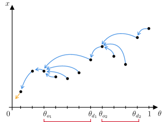
Figure 1: $U$-shaped regions and binding constraints for a fixed allocation rule

As the figure shows, equivalently, the local IC constraints bind until one travels into a $U$-shaped region (beginning with say index $o$) where the binding constraints then point toward $\theta_{o}$. This provides some further intuition about (1), as (1) can then be written as

$$(\mathbf{T}[x])_{i}=u(x_{i},\theta_{i})-\underbrace{\sum_{j=1,2,\dots,i-1:\ j\in Q}\Big{(}u(x_{j},\theta_{j+1})-u(x_{j},\theta_{j})\Big{)}}_{\text{local}}-\underbrace{\sum_{l=1,2,\dots,L:\ o_{l}<i}\Big{(}u(x_{o_{l}},\theta_{\min(d_{l},i)})-u(x_{o_{l}},\theta_{o_{l}})\Big{)}}_{\text{nonlocal}}\,.$$

where $Q$ is the region where $x$ is monotone in an appropriate sense. The first sum arises from the binding local downward IC constraints, and the second sum arises from the binding nonlocal downward IC constraints. If $x$ is monotone, then (4.3) will reduce to the standard transfer formula in one-dimensional screening models, in which only the local downward IC constraints matter (for transfers). However, importantly, we cannot rule out any $x\in\mathcal{X}^{n}$ by implementability here since we do not have upward incentive constraints. The transfer rule $\mathbf{T}[x]$ depends on the shape of the allocation rule $x$.

Proof of Claim 1.

Relax all the constraints in (6) except the ones indicated in Claim 1. We will show the following: First, these constraints must bind in the relaxed problem. Second, these constraints binding imply all downward IC constraints and all IR constraints. Third, there is a unique solution to the system of equations defined by these binding constraints. Claim 1 then follows.

Note that for every $i>1$, there is precisely one corresponding constraint $[i\rightarrow j]$ for some $j$. If this constraint does not bind at some mechanism $(x,t)$, then simply set $\tilde{t}_{i}=t_{i}+\epsilon$ for some $\epsilon>0$ small enough so that $[i\rightarrow j]$ still holds. This clearly increases the objective. It also does not distort other IC constraints. Indeed, the only other IC constraints this change affects are of the form $[k\rightarrow i]$ for some $k$, but

$$u(x_{k},\theta_{k})-t_{k}\geq u(x_{i},\theta_{k})-t_{i}\geq u(x_{i},\theta_{k})-\tilde{t}_{i}\,.$$

Therefore, all the IC constraints identified in Claim 1 must bind. Similarly, $\text{IR}[1]$ binds.

Given that these constraints bind, we now show that they imply all the downward IC constraints in (6). We first collect two lemmas:

Lemma 2 (Local to global).

Let $i>j>k$. If $[i\rightarrow j]$, $[j\rightarrow k]$ hold and $x_{j}\geq x_{k}$, then $[i\rightarrow k]$.

Lemma 3 (Global to local).

Let $i>j>k$. If $[i\rightarrow k]$, $[j\rightarrow k]$ bind and $x_{j}\leq x_{k}$, then $[i\rightarrow j]$.

Lemma 2 is standard; it follows from a revealed-preference argument using the single-crossing property of $u$ (we include a proof in the appendix for completeness). Lemma 3 appears to be new; it requires two binding IC constraints and follows from a revealed-preference argument that subtracts the two constraints. The appendix provides details.

We show all downward IC constraints are satisfied by induction on the number of $U$-shaped regions $L$. When $L=0$, all downward IC constraints hold by successively applying Lemma 2 and building up from the adjacent local downward constraints. Suppose the claim holds for $L-1$. Let us denote the last region as $r$ with starting index $o$ and end index $d$. By the inductive hypothesis, all downward IC constraints $[i\rightarrow j]$ are satisfied if $j<i\leq o$. We divide the remaining pairs $(j,i)$ with $j<i$ into two cases:

• Case (1): $o\leq j<i$. We make the following observations:

  • if $o\leq j<i\leq d$, then $[i\rightarrow j]$ follows by the binding IC constraints $[i\rightarrow o]$, $[j\rightarrow o]$, $x_{j}\leq x_{o}$, and Lemma 3;

  • if $d\leq j<i$, then $[i\rightarrow j]$ follows by successively applying Lemma 2;

  • if $j<d<i$, then $[i\rightarrow j]$ follows by $[i\rightarrow d]$ from (b), $[d\rightarrow j]$ from (a), $x_{d}\geq x_{j}$, and Lemma 2.

• Case (2): $j<o<i$. Note that $x_{j}\leq x_{o}$ for all $j<o$. Then, $[i\rightarrow j]$ follows by $[i\rightarrow o]$ from Case (1), $[o\rightarrow j]$ from the inductive hypothesis, $x_{o}\geq x_{j}$, and Lemma 2.

Together, these cover all the downward IC constraints and prove the inductive step. The IR constraints follow easily from $\text{IR}[1]$ and $\text{IC}[i\rightarrow 1]$ and that $u(x,\,\cdot\,)$ is nondecreasing.

The binding constraints define a system of $n$ equations for $t$. With some calculations, it is not hard to see that these equations can be solved successively starting from the lowest one. In particular, by induction, the solution is uniquely defined by (1). ∎

Step 2:

Consider any feasible $(x,t)$ to (5) that does not satisfy some upward IC constraints. We are now ready to construct a perturbation that strictly improves on $(x,t)$.

There are two cases: (i) $x$ is monotone and (ii) $x$ is not monotone. The first case is simple. As noted before, when $x$ is monotone, $\mathbf{T}[x]$ reduces to the standard transfer formula and hence $(x,\mathbf{T}[x])$ must satisfy all incentive constraints including the upward ones. Then, $t$ cannot be identically equal to $\mathbf{T}[x]$. But that implies $(x,t)$ can be strictly improved by $(x,\mathbf{T}[x])$ by Claim 1.

Consider the second case where $x$ is not monotone. Then, there must exist a $U$-shaped region. Let $r$ be the first $U$-shaped region, $o$ its starting index, and $d$ its end index.

By definition of $\mathbf{T}$, it suffices to construct a perturbation $\tilde{x}$ of $x$ such that $(\tilde{x},\mathbf{T}[\tilde{x}])$ strictly improves upon $(x,\mathbf{T}[x])$. The perturbation we construct will act on a carefully chosen set of types. In particular, let

$$g=\min\big{\{}j>o:x_{j}\geq x_{o}\big{\}}$$

denote the first index after $o$ with associated allocation no less than $x_{o}$. Put $g=n+1$ if the above set is empty. Then, either $g=d$ or $g=n+1$.

Let

$$\hat{x}=\max\big{\{}x_{j}:o<j<g\big{\}}$$

denote the largest allocation for indices strictly between $o$ and $g$. We have $\hat{x}<x_{o}$. Let $j^{*}\in\{o+1,\dots,g-1\}$ be the first index achieving the above maximum and let $\hat{\theta}=\theta_{j^{*}}$.

Let

$$k=\min\big{\{}j:x_{j}>\hat{x}\big{\}}$$

denote the first index whose associated allocation is strictly higher than $\hat{x}$. Since $x_{o}>\hat{x}$, we have $k\leq o$. Because $r$ is the first $U$-shaped region, we have

$$\hat{x}<x_{k}\leq x_{k+1}\leq\cdots\leq x_{o}\,.$$

Consider the following perturbation $\tilde{x}$: for all $j\in\{1,\dots,n\}$,

$$\tilde{x}_{j}:=\begin{cases}\hat{x}&\text{ if }j\in\{k,k+1,\dots,o\}\,;\\ x_{j}&\text{ otherwise.}\\ \end{cases}$$

Figure 2 illustrates.

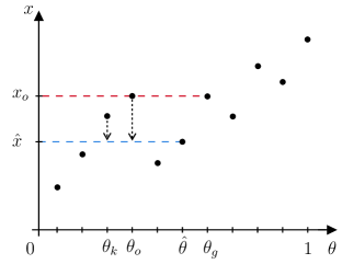
Figure 2: Perturbation of the allocation rule

Claim 2.

The objective of (5) under $(\tilde{x},\mathbf{T}[\tilde{x}])$ is strictly higher than that under $(x,\mathbf{T}[x])$.

Proof of Claim 2.

The main difficulty here is that $\mathbf{T}$ is a complicated operator because of the binding nonlocal incentive constraints. The perturbed allocation $\tilde{x}$ is constructed in such a way that it maintains the form of $\mathbf{T}$ in the following sense. Define function $\varphi:\mathcal{P}(\{1,\dots,n\})\times\mathcal{X}^{n}\rightarrow\mathds{R}^{n}$ by

$$(\varphi(K,a))_{i}:=u(a_{i},\theta_{i})-\sum_{j\in K\cup\{i\}:\,j\leq i}\Big{(}u(a_{\max\{k\in K:k<j\}},\theta_{j})-u(a_{\max\{k\in K:k<j\}},\theta_{\max\{k\in K:k<j\}})\Big{)}$$

for all $i=1,\dots,n$, where $\mathcal{P}(\,\cdot\,)$ is the power set operator. For any allocation rule $a\in\mathcal{X}^{n}$, let $S_{a}$ be the running maximum index set as defined earlier. Then, by (1), $\mathbf{T}[a]=\varphi(S_{a},a)$.

Lemma 4.

Consider any two allocation rules $a,b\in\mathcal{X}^{n}$ with running maximum index sets $S_{a},S_{b}$. Suppose $S_{a}\subseteq S_{b}$, and $b_{i}=b_{\max\{j\in S_{a}:j<\min(S_{b}\backslash S_{a})\}}$ for all $i\in S_{b}\backslash S_{a}$. Then,

$$\mathbf{T}[b]=\varphi(S_{b},b)=\varphi(S_{a},b)\,.$$

The appendix provides the proof of this lemma. Note that by construction $x$, $\tilde{x}$ always satisfy the conditions in Lemma 4. Applying Lemma 4 to $x$, $\tilde{x}$ gives $\mathbf{T}[\tilde{x}]=\varphi(S,\tilde{x})$, where $S$ is the running maximum index set of $x$. We show that the objective of (5), after plugging in $\varphi(S,\,\cdot\,)$, weakly increases on the parts involving $x_{k},x_{k+1},\dots,x_{o-1}$ (which may be an empty set) and strictly increases on the parts involving $x_{o}$ (which always exist).

Fix any $j\in\{k,k+1,\dots,o-1\}$. Plugging $\varphi(S,\,\cdot\,)$ into the objective of (5) and collecting terms involving $x_{j}$ gives

$$s(x_{j},\theta_{j})\mu(\theta_{j})-\big{(}u(x_{j},\theta_{j+1})-u(x_{j},\theta_{j})\big{)}\sum_{i>j}\mu(\theta_{i})\,.$$

Now consider the terms involving $x_{j^{*}}$. Because $o<j^{*}<g$, there is no IC constraint pointing toward $j^{*}$ by Claim 1. Therefore, there is only one such term:

$$s(x_{j^{*}},\theta_{j^{*}})\mu(\theta_{j^{*}})\,.$$

Note that $x_{j}\in\mathcal{X}$ is feasible to assign to $\theta_{j^{*}}$. Moreover, since $x_{j}\leq x_{o}$, doing so maintains the form of $\mathbf{T}$ by Lemma 4, and thus generates a payoff also according to the above formula. The fact that $x$ is optimal then implies

$$s(\hat{x},\hat{\theta})\geq s(x_{j},\hat{\theta})\,;$$

that is,

$$s(x_{j},\hat{\theta})-s(\hat{x},\hat{\theta})\leq 0\,.$$

Because $x_{j}>\hat{x}$ and $\theta_{j}<\hat{\theta}$, by the weak single-crossing differences property of $s$,

$$s(x_{j},\theta_{j})-s(\hat{x},\theta_{j})\leq 0\,.$$

Moreover, because $x_{j}>\hat{x}$, by the strict increasing differences property of $u$,

$$u(x_{j},\theta_{j+1})-u(x_{j},\theta_{j})>u(\hat{x},\theta_{j+1})-u(\hat{x},\theta_{j})\,.$$

Combining (4.3) and (4.3) gives

$$s(x_{j},\theta_{j})\mu(\theta_{j})-\big{(}u(x_{j},\theta_{j+1})-u(x_{j},\theta_{j})\big{)}\sum_{i>j}\mu(\theta_{i})\leq s(\hat{x},\theta_{j})\mu(\theta_{j})-\big{(}u(\hat{x},\theta_{j+1})-u(\hat{x},\theta_{j})\big{)}\sum_{i>j}\mu(\theta_{i})\,,$$

proving that the part of the objective involving $x_{j}$ increases.

Because this holds for all $j\in\{k,k+1,\dots,o-1\}$, to conclude our proof, it remains to show that the part of the objective involving $x_{o}$ strictly increases. Plugging $\varphi(S,\,\cdot\,)$ into (5) and collecting terms involving $x_{o}$ gives

$$s(x_{o},\theta_{o})\mu(\theta_{o})-\sum_{i=o+1}^{g}\mu(\theta_{i})\big{(}u(x_{o},\theta_{i})-u(x_{o},\theta_{o})\big{)}-\big{(}u(x_{o},\theta_{g})-u(x_{o},\theta_{o})\big{)}\sum_{i>g}\mu(\theta_{i})\,.$$

By the same argument as the previous case, we have

$$s(x_{o},\theta_{o})\leq s(\hat{x},\theta_{o})\,.$$

For any $i>o$, by the strict increasing differences property of $u$,

$$u(x_{o},\theta_{i})-u(x_{o},\theta_{o})>u(\hat{x},\theta_{i})-u(\hat{x},\theta_{o})\,.$$

Together they imply

$$s(x_{o},\theta_{o})\mu(\theta_{o})-\sum_{i=o+1}^{g}\mu(\theta_{i})\big{(}u(x_{o},\theta_{i})-u(x_{o},\theta_{o})\big{)}-\big{(}u(x_{o},\theta_{g})-u(x_{o},\theta_{o})\big{)}\sum_{i>g}\mu(\theta_{i})$$

$$<s(\hat{x},\theta_{o})\mu(\theta_{o})-\sum_{i=o+1}^{g}\mu(\theta_{i})\big{(}u(\hat{x},\theta_{i})-u(\hat{x},\theta_{o})\big{)}-\big{(}u(\hat{x},\theta_{g})-u(\hat{x},\theta_{o})\big{)}\sum_{i>g}\mu(\theta_{i})\,,$$

where the strict inequality also uses that $\mu$ has full support. ∎

Step 3:

We prove Theorem 2 for general type space $\Theta$ by approximation. We give a sketch of the argument here and leave the details to the appendix. Let $\mu\in\Delta(\Theta)$ denote the distribution on $\Theta$. Recall that $\eqref{eq:1d}^{\dagger}$ denotes the version of program $\eqref{eq:1d}$ with all IC constraints (both downward and upward). Let $V(\Theta,\mu)$ denote the optimal value of $\eqref{eq:1d}^{\dagger}$ given $(\Theta,\mu)$. We show that $V(\Theta,\mu)$ equals to the optimal value of $\eqref{eq:1d}$. Suppose, for contradiction, there exists some $(\hat{x},\hat{t})$ feasible for $\eqref{eq:1d}$ such that

$$V(\Theta,\mu)<\operatorname{\mathds{E}}^{\mu}[v(\hat{x}(\theta),\theta)+\hat{t}(\theta)]\,.$$

We first construct an appropriate sequence $\{(\Theta^{(n)},\mu^{(n)})\}$ approximating $(\Theta,\mu)$.

Lemma 5.

Suppose $v(x,\theta)$ is Lipschitz continuous on $\mathcal{X}\times\Theta$. Then, there exists a sequence $\{(\Theta^{(n)},\mu^{(n)})\}$ with $\Theta^{(n)}\subseteq\Theta$ finite and $\mu^{(n)}\in\Delta(\Theta^{(n)})$ full support such that

• $\mu^{(n)}\rightarrow_{w}\mu$ ;

• $\displaystyle\limsup_{n\rightarrow\infty}V(\Theta^{(n)},\mu^{(n)})\leq V(\Theta,\mu)$ .

Suppose for a moment that $\hat{x},\hat{t}$ are continuous on $\Theta$ and $v$ is Lipschitz continuous. Note that $(\hat{x},\hat{t})$ restricted to $\Theta^{(n)}$ is a feasible solution to the finite-type version of (4) with $(\Theta^{(n)},\mu^{(n)})$. By Step 2, we have $V(\Theta^{(n)},\mu^{(n)})\geq\operatorname{\mathds{E}}^{\mu^{(n)}}[v(\hat{x}(\theta),\theta)+\hat{t}(\theta)]$. Because $v(\hat{x}(\theta),\theta)+\hat{t}(\theta)$ is a bounded continuous function on $\Theta$, using Lemma 5 and taking limits on both sides of the above, we have

$$V(\Theta,\mu)\geq\limsup_{n\rightarrow\infty}V(\Theta^{(n)},\mu^{(n)})\geq\limsup_{n\rightarrow\infty}\operatorname{\mathds{E}}^{\mu^{(n)}}[v(\hat{x}(\theta),\theta)+\hat{t}(\theta)]=\operatorname{\mathds{E}}^{\mu}[v(\hat{x}(\theta),\theta)+\hat{t}(\theta)]\,,$$

contradicting (4.3). However, the situation is more delicate in general. The proof (in the appendix) relies on the Stone–Weierstrass theorem and Lusin’s theorem.

Finally, to conclude Theorem 2, it suffices to show the existence of an optimal solution to the full IC program $\eqref{eq:1d}^{\dagger}$. Even though this is a standard one-dimensional problem, the existence result appears to be new at this level of generality.

Lemma 6.

Any standard one-dimensional screening problem has a solution.

The proof (in the appendix) proceeds by showing the space of IC and IR mechanisms is sequentially compact in the product topology. The argument uses a generalized version of Helly’s selection theorem from Fuchino and Plewik (1999).

4.4 Reduction

For the more general case of positive correlation (instead of perfect correlation), we reduce it to a set of subproblems each of which has $\theta^{B}=\theta^{A}$. Suppose $\Theta^{B}=\Theta^{A}=[0,1]$ and $\theta^{B}$ is stochastically monotone in $\theta^{A}$. Let $\varepsilon$ be an independent uniform $[0,1]$ draw. Note that the random vector $(\theta^{A},\theta^{B})$ can be simulated by

$$(\theta^{A},\theta^{B})\stackrel{{\scriptstyle d}}{{=}}(\theta^{A},F^{-1}(\varepsilon\mid\theta^{A}))\,,$$

where $F^{-1}(\,\cdot\,|\,\theta^{A})$ is the generalized inverse function of $F(\,\cdot\,|\,\theta^{A})$. Our positive correlation condition states that $\theta^{B}\mid\theta^{A}$ shifts upward in the sense of stochastic dominance as $\theta^{A}$ increases. This implies that $F^{-1}(\varepsilon\,|\,\cdot\,)$ is a nondecreasing function. Therefore, if we reveal the realization of $\varepsilon$ to the principal and let the principal design a mechanism contingent on $\varepsilon$, the problem reduces to the case in which $\theta^{B}=h_{\varepsilon}(\theta^{A})$ for some nondecreasing function $h_{\varepsilon}$. Now, simply define $\tilde{u}^{B}_{\varepsilon}(y,\theta^{A}):=u^{B}(y,h_{\varepsilon}(\theta^{A}))$ and $\tilde{v}^{B}_{\varepsilon}(y,\theta^{A}):=v^{B}(y,h_{\varepsilon}(\theta^{A}))$. For each realization of $\varepsilon$, we can apply our result from the previous two subsections to the screening problem with utility functions $(u^{A},\tilde{u}^{B}_{\varepsilon},v^{A},\tilde{v}^{B}_{\varepsilon})$ and perfect correlation $\theta^{B}=\theta^{A}$. Thus, for each realization of $\varepsilon$, simply screening the productive component is optimal, but that mechanism does not depend on $\varepsilon$ and hence must be optimal in the original problem.

Remark 1.

In the more general case where $\theta^{B}$ is multidimensional, to perform the above reduction, we use an insight due to Haghpanah and Hartline (2021) who make use of a classic result of Strassen (1965) on monotone coupling. For measurability issues, we prove a measurable monotone coupling lemma (see Lemma 7 in Section B.3), building on a result by Kamae and Krengel (1978).

5 Monopoly Pricing with Costly Signals

Before discussing other applications of Theorem 1 in Section 6, we specialize the main model to a setting of monopoly pricing with costly signals. In this setting, a monopolist sells a spectrum of quality-differentiated goods and can make the menu of offers contingent on the costly actions that a buyer may take.

In Section 5.1, we show that if the buyer’s utility functions are multiplicatively separable within each component, then the positive correlation of preferences condition can be weakened to the positive correlation between the preferences for the productive component and the marginal rates of substitution between the productive and costly components.

In Section 5.2, we consider a multiple-good monopolist selling different qualities of bundles (with no costly signals). This environment generalizes the classic multiple-good monopoly problem by allowing for both probabilistic bundling and quality discrimination. We show that (a relaxation of) this problem can be mapped to a monopolist selling a spectrum of quality-differentiated goods without bundling but with costly signals as in Section 5.1. A key insight is that one can view selling the grand bundle as the productive component, and selling a smaller bundle instead of the grand bundle as a costly instrument for screening a consumer’s value for the grand bundle. Using this perspective, we generalize a result of Haghpanah and Hartline (2021). In particular, we show that under their stochastic ratio monotonicity condition, the general feature of the optimal mechanism is to post a menu of different qualities of the grand bundle — the monopolist screens only the productive component and does not use any of the “costly signals.”

Setup.

A monopolist sells a quality-differentiated spectrum of goods. A buyer of type $\theta^{A}\in\Theta^{A}$ receives utility $u^{A}(x,\theta^{A})$ from consuming the good of quality $x\in\mathcal{X}$. The seller incurs a cost $C(x,\theta^{A})$ to produce the good of quality $x$ for type $\theta^{A}$. Suppose $u^{A}(x,\theta^{A})$ is nondecreasing in $\theta^{A}$ and has strict increasing differences, and that the surplus function $u^{A}(x,\theta^{A})-C(x,\theta^{A})$ has weak single-crossing differences. (The continuity and compactness assumptions in Section 2 are also maintained.)

Besides offering a menu of products of different qualities and prices, the monopolist can make the offers contingent on various costly signals (e.g. waiting in line, collecting coupons, walking up stairs). A costly signal is represented by $y\in\mathcal{Y}$. To obtain a signal $y$, a buyer of type $\theta^{B}\in\Theta^{B}$ incurs a cost $c(y,\theta^{B})$ that is nonincreasing in $\theta^{B}$ (so $\theta^{B}$ represents the willingness to endure various costly activities).

Theorem 1 then says that if $\theta^{B}$ is positively correlated with $\theta^{A}$ according to our notion, then the monopolist never makes more profits by using these costly signals. Therefore, if the monopolist in fact uses these instruments, then we should expect that the consumers with higher willingness to pay tend to incur higher costs to obtain the signals (both measured with respect to the constant marginal value for money). In fact, sometimes we can say more when the buyer’s utility functions are multiplicatively separable within each component, which we turn to next.

5.1 Marginal Rates of Substitution Between Two Components

We follow the notation in the above setup, and let $\mathcal{X}$ be $[0,1]$, $\mathcal{Y}$ any measurable space, $\Theta^{A}$ any compact subset of $\mathds{R}_{++}$, and $\Theta^{B}$ any compact subset of $\mathds{R}^{N}_{-}$. We say that the buyer has multiplicatively separable utilities within each additive component if for any quality $x$, signal $y$, and price $t$, the buyer’s payoff can be written as

$$\theta^{A}u(x)+\theta^{B}\cdot c(y)-t\,,$$

where $u:\mathcal{X}\rightarrow\mathds{R}$ is a continuous and strictly increasing function satisfying $u(0)=0$, and $c:\mathcal{Y}\rightarrow\mathds{R}_{+}^{N}$ is a bounded measurable function satisfying $c(y_{0})=0$ for some $y_{0}\in\mathcal{Y}$.

We say that the monopolist’s cost function is not interdependent if $C(x,\theta^{A})$ does not depend on $\theta^{A}$, in which case without loss of generality we let $C(0)=0$.

Recall the notation $\theta^{B}=(\theta^{1},\dots,\theta^{N})$. Let $r^{i}=\frac{\theta^{i}}{\theta^{A}}$ and $r^{B}=(r^{1},\dots,r^{N})$. Note that $r^{B}\leq 0$. We interpret $r^{B}$ as the (negative) marginal rates of substitution between the productive and costly components. In this setting, we show that our assumption of positive correlation between $\theta^{A}$ and $\theta^{B}$ can be weakened to that between $\theta^{A}$ and $r^{B}$.

Proposition 2.

Suppose the seller’s cost function $C$ is continuous, nondecreasing in $x$, and not interdependent; the buyer’s utilities are multiplicatively separable; and $r^{B}$ is stochastically nondecreasing in $\theta^{A}$. Then, there exists an optimal mechanism that involves no costly screening.

The intuition behind this result can be understood in the same way as in the proof of the main result (Section 4). We show that when the marginal rates of substitution are increasing in the values, instead of using the costly signals, the principal can simply adjust the allocations of the productive component while maintaining the downward IC constraints. Because downward IC constraints are sufficient, the result follows. Unlike in Section 4, in this case we substitute the costly signals with a decrease in the productive allocations holding the monetary transfers fixed, which is why the marginal rates of substitution between the two components play an important role here.

Proof of 2.

By Lemma 7 in Section B.3, as in Section 4.4, it suffices to show the case where $r^{B}=h(\theta^{A})$ for some nondecreasing function $h:\Theta^{A}\rightarrow\mathds{R}^{N}$. Thus, we may assume for all $i$, $r^{i}$ is deterministic conditional on $\theta^{A}$ and nondecreasing in $\theta^{A}$. Fix any $(x,y,t)$ that is IC and IR. We may assume $t\geq 0$, because the monopolist can simply replace all options with negative profits in the menu with $(0,y_{0},0)$ and weakly increase the total profit (since the monopolist’s cost function does not depend on the buyer’s type). Now we apply a reconstruction argument as follows. Consider the modification: $\tilde{t}=t,\tilde{y}=y_{0}$,

$$\tilde{x}(\theta)=u^{-1}\big{(}u(x(\theta))+\frac{1}{\theta^{A}}[\theta^{B}\cdot c(y(\theta))]\big{)}\,.$$

Because $u(\,\cdot\,)$ is continuous and strictly increasing with $u(0)=0$, $u^{-1}$ is defined on $[0,u(1)]$. Moreover, because $(x,y,t)$ is IR and $t\geq 0$, we have $0\leq u(x(\theta))+\frac{1}{\theta^{A}}[\theta^{B}\cdot c(y(\theta))]\leq u(x(\theta))$ for all $\theta$. So the modification is well-defined and $0\leq\tilde{x}\leq x$ pointwise. In other words, the modified mechanism decreases the productive allocation to substitute the costly screening so that all types have the same utilities as before, assuming truthful reporting.

Because $C(\,\cdot\,)$ is nondecreasing, this modification increases the objective, assuming truthful reporting. It is IR by construction. Moreover, it is downward IC: for any $\hat{\theta}^{A}<\theta^{A}$,

$$\theta^{A}u(\tilde{x}(\theta))-\tilde{t}(\theta) =\theta^{A}u(x(\theta))+\theta^{B}\cdot c(y(\theta))-t(\theta)$$

$$\geq\theta^{A}u(x(\hat{\theta}))+\theta^{B}\cdot c(y(\hat{\theta}))-t(\hat{\theta})$$

$$=\theta^{A}\big{(}u(x(\hat{\theta}))+r^{B}\cdot c(y(\hat{\theta}))\big{)}-t(\hat{\theta})$$

$$\geq\theta^{A}\big{(}u(x(\hat{\theta}))+\hat{r}^{B}\cdot c(y(\hat{\theta}))\big{)}-t(\hat{\theta})=\theta^{A}u(\tilde{x}(\hat{\theta}))-\tilde{t}(\hat{\theta})\,.$$

The first inequality holds because $(x,y,t)$ is IC. The second inequality holds because $\hat{r}^{B}\leq r^{B}$ and $c\geq 0$. Invoking Theorem 2 concludes the proof. ∎

5.2 Bundling and Quality Discrimination

We now show an application to a multiple-good monopoly problem allowing for both probabilistic bundling and quality discrimination.

A monopolist sells $G$ many goods to a unit mass of consumers. For each bundle $b$, a random consumer has value $v^{b}$ for getting the highest quality version of the bundle with probability one. We assume that $v^{b}\leq v^{b^{\prime}}$ for all $b\subset b^{\prime}$ and $v^{\varnothing}=0$. The monopolist can use probabilistic bundling, captured by a bundling allocation rule $v\mapsto\alpha(v)\in\Delta(2^{G})$. In addition, the monopolist can adjust the quality of each bundle, captured by a quality allocation rule $v\mapsto q(v)\in[0,1]^{2^{G}}$. A type-$v$ consumer’s payoff is given by

$$\sum_{b}\alpha^{b}q^{b}v^{b}-t\,.$$

The monopolist incurs a cost to improve the quality of a bundle, with a payoff given by

$$-\sum_{b}\alpha^{b}C(q^{b})+t\,,$$

where $C(\,\cdot\,)$ is a continuous, nondecreasing, and convex function on $[0,1]$ with $C(0)=0$. This cost structure assumes that the cost of producing a bundle of some quality does not depend on the size of the bundle, which is perhaps more suitable for digital goods.

Let $v^{*}$ be the value of a random consumer for the grand bundle and $\tau=(\frac{v^{b}}{v^{*}})_{b=1,\dots,2^{G}}$ be the profile of values for each bundle relative to the grand bundle.

Proposition 3.

If $\tau$ is stochastically nondecreasing in $v^{*}$, then an optimal mechanism exists and can be implemented by a menu of prices for different qualities of the grand bundle.

This result is a natural consequence of 2 once one views selling the grand bundle as the productive component, and selling a smaller bundle instead of the grand bundle as a costly instrument for screening a consumer’s value for the grand bundle.

Proof of 3.

By convexity of $C(\,\cdot\,)$ and Jensen’s inequality, we have

$$\sum_{b}\alpha^{b}(v)C(q^{b}(v))\geq C\Big{(}\sum_{b}\alpha^{b}(v)q^{b}(v)\Big{)}\,.$$

Therefore, it is an upper bound on the monopolist’s revenue to maximize the objective

$$\operatorname{\mathds{E}}\Big{[}-C\Big{(}\sum_{b}\alpha^{b}(v)q^{b}(v)\Big{)}+t(v)\Big{]}\,.$$

For this auxiliary problem, let us also relax the constraint $\sum_{b}\alpha^{b}=1$ to $\sum_{b}\alpha^{b}\leq 1$. Then, because $\alpha,q$ enter both the consumer’s utility and the objective in the same way, it is without loss of generality to let $q^{b}=1$ for all $b$.

We now reformulate this problem as a problem of monopoly pricing with costly signals. Let $\theta^{A}=v^{*}$ be the value of the grand bundle. For any proper bundle $b$, let

$$\theta^{b}=v^{b}-v^{*}$$

be the difference of values for bundle $b$ and the grand bundle $b^{*}$. In words, $\theta^{b}$ is the negative value for getting bundle $b$ instead of $b^{*}$. Let $N=2^{G}-1$, and let $\theta^{B}=(\theta^{1},\dots,\theta^{N})$ be the profile of the differences.

We use $x:\Theta\rightarrow[0,1]$ to denote the initial allocation of the grand bundle, and $y:\Theta\rightarrow[0,1]^{N}$ to denote the allocation of the “costly signals” as follows. An assignment $y^{b}\in[0,1]$ represents assigning bundle $b$ with probability $y^{b}$ while decreasing the probability of the grand bundle $b^{*}$ also by $y^{b}$. The consumer’s payoff can be rewritten as

$$\theta^{A}x+\theta^{B}\cdot y-t\,.$$

For any substochastic allocation $\alpha$ (i.e. $\sum_{b}\alpha_{b}\leq 1$), we can replicate it by setting

$$x=\sum_{b}\alpha^{b}\,,\qquad y^{b}=\alpha^{b}\text{ for all }b\neq b^{*}\,.$$

Therefore, the auxiliary problem (5.2) can be further relaxed to

$$\sup_{(x,y,t)\in\mathcal{M}(\Theta)}\operatorname{\mathds{E}}[-C(x(\theta))+t(\theta)]\,.$$

For any $b=1,\dots,N$, we have $\frac{v^{b}}{v^{*}}=\frac{\theta^{A}+\theta^{b}}{\theta^{A}}=1+\frac{\theta^{b}}{\theta^{A}}$. Since $\tau$ is stochastically nondecreasing in $v^{*}$, we have $r^{B}:=\frac{1}{\theta^{A}}\theta^{B}$ is stochastically nondecreasing in $\theta^{A}$. So 2 applies to (5.2). Let $(x^{*},0,t^{*})$ be the optimal solution to (5.2) that involves no costly screening.

We construct an allocation rule in the original problem as follows:

$$\alpha^{b^{*}}=1 \alpha^{b}=0 b\neq b^{*} q^{b^{*}}=x^{*} q^{b}=0 b\neq b^{*}$$, for all ;  , for all .

Because probabilities and qualities enter the consumer’s utility in the same way and $(x^{*},0,t^{*})$ is IC and IR, $(\alpha,q,t^{*})$ is also IC and IR. The revenue of the monopolist under $(\alpha,q,t^{*})$ is

$$\operatorname{\mathds{E}}[-C(q^{b^{*}}(\theta))+t^{*}(\theta)]=\operatorname{\mathds{E}}[-C(x^{*}(\theta))+t^{*}(\theta)]\,,$$

the optimal value of (5.2). Hence, $(\alpha,q,t^{*})$ is optimal for the monopolist in the original problem; moreover, $(\alpha,q,t^{*})$ screens using only the qualities of the grand bundle. ∎

Remark 2.

3 says that under the stochastic ratio monotonicity condition, the monopolist can restrict attention to selling only the grand bundle at various qualities. Because that is a one-dimensional problem à la Mussa and Rosen (1978), the solution can be explicitly characterized. When there is no cost for quality improvement ($C=0$), the optimal mechanism is to sell the grand bundle at the highest quality with a posted price. This special case is due to Haghpanah and Hartline (2021). In general, however, the optimal mechanism involves price discrimination. But 3 shows that such price discrimination is only done by creating different qualities of the grand bundle.

6 Additional Applications

6.1 Bundling with Nested Bundles

Complementary to Section 5.2, rather than quality discrimination, companies may also offer a menu of bundles that are nested (e.g. cable TV providers offer a basic package and a premium package including sports channels). Bergemann et al. (2021) refer to such selling strategies as upgrade pricing and provide sufficient conditions under which they are optimal when consumers have additive values. We provide a different set of sufficient conditions on the optimality of upgrade pricing with non-additive values, as an application of our main result.

For this application, we restrict attention to one-dimensional types $\theta\in\Theta\subset\mathds{R}$ and deterministic bundling mechanisms. For example, consider two items $\{1,2\}$. Let $g(\theta)$, $h(\theta)$, and $v(\theta)$ be the value of item $1$, the value of item $2$, and the value of the bundle $\{1,2\}$ for type $\theta$, respectively. We assume that $g,h,v$ are continuous, nondecreasing in $\theta$ (e.g. $\theta$ represents income), and that $v(\theta)\geq\max\{g(\theta),h(\theta)\}$ (e.g. there is free disposal).

Proposition 4.

If $v(\theta)-g(\theta)$ is strictly increasing, and $v(\theta)-h(\theta)$ is nonincreasing, then an optimal mechanism exists and can be implemented with a menu of nested bundles $\{\{1\},\{1,2\}\}$.

In terms of the cable TV service example, this result says that if a higher-income consumer has a higher incremental value for sports channels, and a lower incremental value for basic channels, then it suffices for the seller to consider a two-tier menu that features a basic package and a premium package including sports channels. This result holds for any distribution of $\theta$. Despite its seeming simplicity, it cannot be derived with any known result in the literature (see Section B.1 for a parametric example).

This result is an immediate consequence of Theorem 1 provided that one takes the same point of view as in Section 5 by considering selling item $2$ instead of the bundle $\{1,2\}$ as a costly instrument. It is not hard to see that any menu of nested bundles that does not include the grand bundle cannot be optimal. For any number of items and any menu of nested bundles that includes the grand bundle, in Section B.1, we provide sufficient conditions under which the menu constitutes an optimal selling mechanism.

6.2 Intertemporal Price Discrimination with Private Discounting

Let $D:\mathcal{R}\times\mathcal{T}\rightarrow[0,1]$ be a general discount function, where $\mathcal{R}\subset\mathds{R}_{+}$ is a compact set of discount rates $r$, and $\mathcal{T}\subset\mathds{R}_{+}$ is a finite set of delivery dates $T$ including $0$. The discount function $D(r,T)$ is nonincreasing in $r$, with $D(r,0)=1$. For example, $D(r,T)=e^{-rT}$ under exponential discounting and $D(r,T)=\frac{1}{1+rT}$ under hyperbolic discounting.

The buyer privately observes his discount rate $r$ and value $v$, with a payoff given by

$$D(r,T)vu(x)-p\,,$$

where $x\in[0,1]$ is the quality of the good and $p\in\mathds{R}$ is the price at time $0$. We assume that $u$ is continuous, strictly increasing, and satisfies $u(0)=0$.

The seller has a continuous, nondecreasing cost $C(x)$ for producing the good of quality $x$. She wants to design an optimal selling mechanism $(x,T,p)$ that specifies the quality, delivery time, and payment for each reported type. A mechanism involves no intertemporal price discrimination if $T(v,r)=0$ for all $v,r$.

The next example shows that if a buyer who has a higher value tends to be less patient, then intertemporal price discrimination can be profitable:

Example 4.

Suppose $\mathcal{T}=\{0,1\}$ and $\mathcal{R}=\{0,r_{1}\}$, where $D(0,1)=1$ and $D(r_{1},1)=\frac{1}{2}$. Suppose $u(x)=x$ and $C(x)=0$. The buyer has equal probabilities of having either $r=0$ or $r=r_{1}$. If $r=0$, then the buyer’s value $v$ is drawn from uniform $[0,1]$. If $r=r_{1}$, then the buyer’s value $v$ is drawn from uniform $[1,2]$. Without intertemporal price discrimination, the seller’s optimal strategy is a posted price $p=1$ which yields payoff $\frac{1}{2}$. However, consider offering $p=1$ for the no-delay option, and $p=\frac{1}{2}$ for the delayed option. Note that all types with $r=r_{1}$ choose the no-delay option, and all types with $r=0$ and $v\geq\frac{1}{2}$ choose the delayed option. This yields the seller payoff $\frac{1}{2}\times 1+\frac{1}{2}\times\frac{1}{2}\times\frac{1}{2}=\frac{5}{8}>\frac{1}{2}$. ∎

The next result shows that if a buyer who has a higher value tends to be more patient, then intertemporal price discrimination is unprofitable:

Proposition 5.

If $r$ is stochastically nonincreasing in $v$, then an optimal mechanism exists and involves no intertemporal price discrimination.

This result is an immediate consequence of 2. This result does not restrict the marginal distributions of $r$ and $v$, but only requires a condition on their joint distribution. Stokey (1979)’s classic result can be seen as a special case of this result with $r$ being a constant (all types have the same patience), $D(r,T)=e^{-rT}$, $u(x)=x$, and $C(x)=0$. Our result shows that whether intertemporal price discrimination is profitable depends on the correlation of consumers’ values and patience.

6.3 Labor Market Screening

A monopsonistic firm wants to hire a worker to perform a task. The firm gets a payoff $V(\theta)$ for hiring a worker of ability $\theta\in\Theta\subset\mathds{R}$, where $V$ is continuous, nondecreasing in $\theta$. The worker suffers a cost $C(\theta)$ for performing the task, where $C$ is continuous, strictly decreasing in $\theta$. Let $x\in[0,1]$ be the probability of hiring the worker.

The firm can ask the applicant to obtain a credential. Suppose that it costs $cy$ to the worker to obtain a $y\in[0,1]$-level credential. Both $\theta$ and $c$ are the worker’s private information. For a given wage level $w$, hiring probability $x$, and credential level $y$, the firm’s payoff is $(V(\theta)-w)x$, and the worker’s payoff is $(w-C(\theta))x-cy$.

Proposition 6.

If $c$ is stochastically nonincreasing in $\theta$, then an optimal mechanism exists and does not require any credential.

This result is an immediate consequence of Theorem 1. This result contrasts with the common perception of costly signals in competitive labor markets (Spence 1973a). To clarify, in Section B.2, we consider a competitive screening model in which multiple firms compete and are allowed to screen with both work allocations and costly instruments. We show that costly screening can appear in equilibrium. The intuition is that with outside options generated through competition, the binding incentive constraints become the upward ones, which is exactly the opposite to the monopsonistic case.

7 Related Literature

This paper proposes a unified mechanism design framework allowing for both price and nonprice screening instruments, characterizes the exact optimum in a general multidimensional screening model, and bridges costly screening and multidimensional screening to obtain new insights into applications such as bundling and price discrimination.

Costly Screening.

Several previous papers have analyzed mechanism design with a costly instrument when monetary transfers are limited or not feasible. In his pioneering study, Banerjee (1997) studies how a bureaucracy can use red tape as an effective screening device when agents are budget-constrained. A recent line of work studies the design of surplus-maximizing mechanisms when monetary transfers are not feasible and agents engage in a one-dimensional costly activity (Hartline and Roughgarden 2008, Condorelli 2012, Chakravarty and Kaplan 2013). We study a profit-maximizing mechanism design problem allowing for both flexible transfers and heterogeneous preferences over costly actions. These features together, in contrast to past work, imply that our model necessarily has multiple screening instruments and requires analysis significantly different from the single-dimensional case.

Multidimensional Screening.

The structure of multidimensional screening differs significantly from its single-dimensional counterpart and remains elusive to fully characterize despite much research over the past decades (Rochet and Stole 2003). Much of the literature focuses on the multiple-good monopoly problem. When there is a single good, the optimal mechanism is simply a posted price (Myerson 1981, Riley and Zeckhauser 1983). However, as soon as there is more than one good, seemingly simple special cases remain poorly understood. Significant progress has been made in developing duality approaches to certify optimality of candidate mechanisms (Rochet and Chone 1998, Daskalakis et al. 2017; Cai et al. 2016, Carroll 2017). In response to the analytical difficulty, several recent papers study either approximately optimal mechanisms (Babaioff et al. 2014, Cai et al. 2016, Hart and Nisan 2017), or worst-case optimal mechanisms (Carroll 2017, Che and Zhong 2021, Deb and Roesler 2021).

In contrast to past work, we consider a multidimensional screening model in which all dimensions except one are surplus destructive. The multiple-good monopoly problem can be viewed as a special case of our framework by redefining the allocation space. Using this perspective, we obtain new insights into bundling, quality discrimination, upgrade pricing, and intertemporal price discrimination.

Our proof method uses a novel nonlocal approach, different from both the Myersonian approach commonly used in the one-dimensional settings and the duality approach commonly used in the multidimensional settings. For a given multidimensional mechanism, we reconstruct an alternative, one-dimensional mechanism that satisfies all downward incentive constraints. We then show via a variational argument that the set of downward incentive constraints is sufficient for one-dimensional screening problems satisfying the surplus condition. Because of the multidimensionality of the screening instruments (i.e. price and nonprice), the main difficulty of our problem appears already when the agent has one-dimensional types. To deduce the more general case, our proof builds on the insight of Haghpanah and Hartline (2021) who make use of Strassen’s theorem to decompose a multidimensional type space. When proving their result, Haghpanah and Hartline (2021) explicitly construct a set of dual variables that only place weights on downward constraints — the existence of such dual variables can be seen as a special case of our main technical result, the downward sufficiency theorem, which states that only downward incentive constraints are needed in one-dimensional models.

Damaged Goods.

There is a line of work studying damaged goods and the profitability of price discrimination (or pure bundling) (Deneckere and McAfee 1996, Anderson and Dana Jr 2009, Haghpanah and Hartline 2021, Ghili forthcoming). A key difference between our result and the results obtained in this literature is that our framework distinguishes between different kinds of damage (e.g. reducing quality vs. requiring waiting) and characterizes when to use which kind of damage. For example, in our bundling application, quality discrimination is used but mixed bundling is not used under the optimal mechanism; in our intertemporal price discrimination application, quality discrimination is used but delay is not used under the optimal mechanism. This is also the reason why our framework allows us to characterize when it is optimal to sell a given menu of nested bundles, a selling strategy necessarily involving damages.

8 Conclusion

This paper studies the effectiveness of costly instruments in a general multidimensional screening model. The model consists of two components: a one-dimensional productive component and a multidimensional costly component. Our main result says that if the agent’s preferences are positively correlated between the two components in a suitably defined sense, then the costly instruments are ineffective — the optimal mechanism simply screens the one-dimensional productive component.

Our proof provides clear insights into why this result holds. First, we show that costly instruments can loosen upward but not downward IC constraints on the costly component. Next, we show that positive correlation of preferences then converts the IC constraints on the costly component to those on the productive component without changing the direction. Finally, we show that the set of downward IC constraints is sufficient for any one-dimensional screening problem satisfying the surplus condition. Therefore, costly instruments cannot help the principal when the agent’s preferences are positively correlated between the two components.

Armed with this understanding, we have also shown how additional results follow naturally. With negatively correlated preferences, we show a partial converse. With multiplicatively separable preferences within each component, we show a stronger result in terms of the marginal rates of substitution between the two components. Using the perspective of screening with costly instruments, as applications, we also provide new insights into multiproduct pricing (bundling, quality discrimination, upgrade pricing), intertemporal price discrimination, and labor market screening.

Appendix A Omitted Proofs

Proof of 1.

Without loss of generality, we may assume $i=1$. Let $v^{A}=v^{B}=0$. Because $\theta^{0}$ has a continuous distribution, there exists some constant $m^{0}$ such that

$$\mathds{P}(\theta^{0}>m^{0})=\mathds{P}(\theta^{0}\leq m^{0})=\frac{1}{2}\,.$$

Similarly define $m^{1}$ for $\theta^{1}$. Since $\theta^{1}$ is stochastically nonincreasing in $\theta^{0}$, we have $\theta^{1}$ and $-\theta^{0}$ are positively upper orthant dependent (Müller and Stoyan 2002, pp. 121-125), and hence

$$\mathds{P}(-\theta^{0}>-m^{0},\theta^{1}>m^{1})\geq\mathds{P}(-\theta^{0}>-m^{0})\mathds{P}(\theta^{1}>m^{1})=\frac{1}{4}\,.$$

Because $\beta(\theta^{0})$, $\beta(\theta^{1})$ are not independent, we have

$$\mathds{P}(\theta^{0}<m^{0},\theta^{1}>m^{1})>\frac{1}{4}$$

and thus

$$\mathds{P}(\theta^{0}>m^{0},\theta^{1}<m^{1})>\frac{1}{4}\,.$$

Define

$$f(\theta^{0})=\begin{cases}1&\text{if $\theta^{0}\leq m^{0}$}\\ 2&\text{if $\theta^{0}>m^{0}$}\end{cases}\,,\qquad g(\theta^{1})=\begin{cases}-1&\text{if $\theta^{1}\leq m^{1}$}\\ -\epsilon&\text{if $\theta^{1}>m^{1}$}\end{cases}\,,$$

where $\epsilon>0$ will be determined shortly. Let $\tilde{f}$ be a continuous approximation of $f$ such that $\tilde{f}(\theta^{0})=f(\theta^{0})$ for all $\theta^{0}\not\in(m^{0}-\epsilon,m^{0}+\epsilon)$. It is clear that we may select $\tilde{f}$ to be nondecreasing. Let $x_{0}=\min\mathcal{X}$ and $\hat{x}=\max\mathcal{X}$. Since $|\mathcal{X}|>1$, $\hat{x}\neq x_{0}$. Since $|\mathcal{Y}|>1$, there exists some $\hat{y}\neq y_{0}\in\mathcal{Y}$. Now let

$$u^{A}(x,\theta^{A})=\tilde{f}(\theta^{0})\frac{x-x_{0}}{\hat{x}-x_{0}},\qquad u^{B}(y,\theta^{B})=g(\theta^{1})\mathds{1}_{y\neq y_{0}}\,.$$

This construction gives admissible utility functions. Consider offering the following menu of three options:

$$\big{\{}(\hat{x},y_{0},2-\epsilon),(\hat{x},\hat{y},1-\epsilon),(x_{0},y_{0},0)\big{\}}\,.$$

Let the agent choose among these, breaking tie in favor of the principal. This yields a payoff of at least

$$r(\epsilon):=(1-\epsilon)\mathds{P}(\theta^{1}>m^{1})+(2-\epsilon)\mathds{P}(\theta^{0}\geq m^{0}+\epsilon,\theta^{1}\leq m^{1})$$

for the principal. Screening the productive component alone yields a payoff of at most

$$q(\epsilon):=2\mathds{P}(m^{0}-\epsilon\leq\theta^{0}\leq m^{0}+\epsilon)+1$$

for the principal. Note that $r(\epsilon),q(\epsilon)$ are both continuous on $(0,\frac{1}{2})$, and

$$\lim_{\epsilon\downarrow 0}r(\epsilon)=\frac{1}{2}+2\mathds{P}(\theta^{0}>m^{0},\theta^{1}<m^{1})>1=\lim_{\epsilon\downarrow 0}q(\epsilon)\,.$$

Thus, there exists some $\epsilon^{*}>0$ such that $r(\epsilon^{*})>q(\epsilon^{*})$. With this choice of $\epsilon^{*}$, the above construction then gives admissible utility functions such that the menu of three options strictly dominates any mechanism screening only the productive component. ∎

Proof of Lemma 2.

Write out $[i\rightarrow j]$ and $[j\rightarrow k]$:

$$u(x_{i},\theta_{i})-t_{i}\geq u(x_{j},\theta_{i})-t_{j}\,;$$

$$u(x_{j},\theta_{j})-t_{j}\geq u(x_{k},\theta_{j})-t_{k}\,.$$

Adding these two yields

$$u(x_{i},\theta_{i})-t_{i}+u(x_{j},\theta_{j})-t_{j}\geq u(x_{j},\theta_{i})-t_{j}+u(x_{k},\theta_{j})-t_{k}\,.$$

Hence,

$$u(x_{i},\theta_{i})-t_{i}\geq(u(x_{j},\theta_{i})+u(x_{k},\theta_{j})-u(x_{j},\theta_{j}))-t_{k}\,.$$

Using $x_{j}\geq x_{k}$, $\theta_{i}>\theta_{j}$, and the strict increasing differences property of $u$, we have

$$u(x_{j},\theta_{i})+u(x_{k},\theta_{j})-u(x_{j},\theta_{j})\geq u(x_{k},\theta_{i})\,.$$

Thus $[i\rightarrow k]$ follows. ∎

Proof of Lemma 3.

Write out the binding constraints $[i\rightarrow k]$ and $[j\rightarrow k]$:

$$u(x_{i},\theta_{i})-t_{i}=u(x_{k},\theta_{i})-t_{k}\,;$$

$$u(x_{j},\theta_{j})-t_{j}=u(x_{k},\theta_{j})-t_{k}\,.$$

Subtracting these two yields

$$u(x_{i},\theta_{i})-u(x_{j},\theta_{j})-t_{i}=u(x_{k},\theta_{i})-u(x_{k},\theta_{j})-t_{j}\,.$$

Hence,

$$u(x_{i},\theta_{i})-t_{i}=(u(x_{j},\theta_{j})+u(x_{k},\theta_{i})-u(x_{k},\theta_{j}))-t_{j}\,.$$

Using $x_{k}\geq x_{j}$, $\theta_{i}>\theta_{j}$, and the strict increasing differences property of $u$, we have

$$u(x_{j},\theta_{j})+u(x_{k},\theta_{i})-u(x_{k},\theta_{j})\geq u(x_{j},\theta_{i})\,.$$

Thus $[i\rightarrow j]$ follows. ∎

Proof of Lemma 4.

Fix any subset $K\subset\{1,\dots,n\}$, any index $k\not\in K$, and any allocation rule $a\in\mathds{R}^{n}$. We claim that if $a_{k}=a_{\max\{j\in K:j<k\}}$, then

$$\varphi(K\cup\{k\},a)=\varphi(K,a)\,.$$

Let $i,i^{\prime}$ be the two consecutive indices in $K$ such that $i<k<i^{\prime}$. Note that for any $j\leq k$,

$$(\varphi(K\cup\{k\},a))_{j}=(\varphi(K,a))_{j}\,,$$

since $(K\cup\{k\})\cap\{j^{\prime}:j^{\prime}<j\}=K\cap\{j^{\prime}:j^{\prime}<j\}$. For any $k<j\leq i^{\prime}$, we can write

$$u(a_{k},\theta_{j})-u(a_{k},\theta_{k})+u(a_{i},\theta_{k})-u(a_{i},\theta_{i})=u(a_{k},\theta_{j})-u(a_{i},\theta_{i})=u(a_{i},\theta_{j})-u(a_{i},\theta_{i})\,,$$

and $i=\max\{j^{\prime}\in K:j^{\prime}<j\}$. Thus $(\varphi(K\cup\{k\},a))_{j}=(\varphi(K,a))_{j}$ for any $k<j\leq i^{\prime}$. Also, the fact that the above holds for $j=i^{\prime}$ implies that $(\varphi(K\cup\{k\},a))_{j}=(\varphi(K,a))_{j}$ for any $j>i^{\prime}$.

Now, write $S_{b}=S_{a}\cup\{k_{1},\dots,k_{m}\}$ with $k_{1}\leq\dots\leq k_{m}$. By assumption, $b_{k_{m}}=\dots=b_{k_{1}}=b_{\max\{j\in S_{a}:j<k_{1}\}}$. Then, by the definition of $S_{b}$, for all $q=2,\dots,m$, we have

$$b_{k_{q}}=b_{\max\{j\in S_{a}\cup\{k_{1},\dots,k_{q-1}\}:j<k_{q}\}}\,.$$

Thus, we can repeatedly apply the result from the previous paragraph and obtain

$$\mathbf{T}[b]=\varphi(S_{a}\cup\{k_{1},\dots,k_{m}\},b)=\varphi(S_{a}\cup\{k_{1},\dots,k_{m-1}\},b)=\dots=\varphi(S_{a}\cup\{k_{1}\},b)=\varphi(S_{a},b)\,,$$

which proves the lemma. ∎

Proof of Lemma 5.

We maintain the notation of Step 3 in Section 4.3. Without loss, let $\Theta\subseteq[0,1)$ and $0\in\Theta$. The construction works as follows. Fix any $n\in\mathds{N}$. Partition $[0,1)$ into intervals $\{[\frac{i-1}{n},\frac{i}{n})\}_{i=1,\dots,n}$. Let

$$I=\Big{\{}i:\mu([\frac{i-1}{n},\frac{i}{n}))>0\Big{\}}\,.$$

For any $i\in I$, let

$$\theta^{(n)}_{i}=\min\Big{\{}[\frac{i-1}{n},\frac{i}{n})\cap\Theta\Big{\}}\,.$$

(The minimum is attained since $\Theta$ is compact.) For notational convenience, we reindex $i$ so that it runs over from $1$ to $|I|$. Let

$$\Theta^{(n)}=\{\theta^{(n)}_{i}\}_{i\in I}\,;$$

$$\mu^{(n)}(\theta^{(n)}_{i})=\mu([\theta^{(n)}_{i},\theta^{(n)}_{i+1}))\,.$$

We have $\Theta^{(n)}\subseteq\Theta$ finite and $\mu^{(n)}\in\Delta(\Theta^{(n)})$ full support. Note that

$$\mu(\{\theta\in\Theta:\theta\in[\theta^{(n)}_{i},\theta^{(n)}_{i+1})\text{ and }|\theta-\theta^{(n)}_{i}|>\frac{1}{n}\})=0\,.$$

We first show property $(ii)$ in the statement. Recall that for this lemma we assume $v$ is Lipschitz continuous on $\mathcal{X}\times\Theta$. Then, there exists some constant $K>0$ such that for any $\theta,\theta^{\prime}\in\Theta$,

$$\max_{x\in\mathcal{X}}|v(x,\theta^{\prime})-v(x,\theta)|\leq K|\theta^{\prime}-\theta|\,.$$

Let $(x^{(n)},t^{(n)})$ be any optimal solution to the full IC program $\eqref{eq:1d}^{\dagger}$ with $(\Theta^{(n)},\mu^{(n)})$. Let $\bar{x}^{(n)}$ be the extension of $x^{(n)}$ to the right:

$$\bar{x}^{(n)}(\theta)=x^{(n)}(\theta^{(n)}_{i})\quad\text{for all }\theta\in[\theta^{(n)}_{i},\theta^{(n)}_{i+1})\,.$$

Note that $\bar{x}^{(n)}$ is a monotonic function on $[0,1)$. Define $\bar{t}^{(n)}$ in the same way. We claim $(\bar{x}^{(n)},\bar{t}^{(n)})$, when restricted to $\Theta$, is a feasible solution to $\eqref{eq:1d}^{\dagger}$ with $(\Theta,\mu)$. To see this, offer the menu $\{(x^{(n)}_{i},t^{(n)}_{i})\}_{i\in I}$ to all types in $\Theta$. Type $\theta^{(n)}_{i+1}$ is indifferent between $(x^{(n)}_{i+1},t^{(n)}_{i+1})$ and $(x^{(n)}_{i},t^{(n)}_{i})$. Type $\theta^{(n)}_{i}$ finds $(x^{(n)}_{i},t^{(n)}_{i})$ optimal. Therefore, any type $\theta$ between $\theta^{(n)}_{i}$ and $\theta^{(n)}_{i+1}$ finds $(x^{(n)}_{i},t^{(n)}_{i})$ optimal since $u$ has strict increasing differences. By construction,

$$V(\Theta^{(n)},\mu^{(n)})=\operatorname{\mathds{E}}^{\mu^{(n)}}[v(\bar{x}^{(n)}(\theta),\theta)+\bar{t}^{(n)}(\theta)]\,.$$

Since $(\bar{x},\bar{t})$ is feasible to $\eqref{eq:1d}^{\dagger}$ with $(\Theta,\mu)$, we have

$$V(\Theta,\mu)\geq\operatorname{\mathds{E}}^{\mu}[v(\bar{x}^{(n)}(\theta),\theta)+\bar{t}^{(n)}(\theta)]\,.$$

Because $\bar{x}^{(n)},\bar{t}^{(n)}$ are constant over each interval $[\theta^{(n)}_{i},\theta^{(n)}_{i+1})$, by (A) and (A), we have

$$\Big{|}\operatorname{\mathds{E}}^{\mu}[v(\bar{x}^{(n)}(\theta),\theta)+\bar{t}^{(n)}(\theta)]-\operatorname{\mathds{E}}^{\mu^{(n)}}[v(\bar{x}^{(n)}(\theta),\theta)+\bar{t}^{(n)}(\theta)]\Big{|}$$

$$=\Big{|}\int v(\bar{x}^{(n)}(\theta),\theta)\mathop{}\!\mathrm{d}\mu-\int v(\bar{x}^{(n)}(\theta),\theta)\mathop{}\!\mathrm{d}\mu^{(n)}\Big{|}$$

$$\leq\sum_{i\in I}\mu^{(n)}(\theta^{(n)}_{i})\sup_{\theta\in[\theta^{(n)}_{i},\theta^{(n)}_{i}+\frac{1}{n}]\cap\Theta}\Big{\{}\max_{x\in\mathcal{X}}\big{|}v(x,\theta)-v(x,\theta^{(n)}_{i})\big{|}\Big{\}}$$

$$\leq\sum_{i\in I}\mu^{(n)}(\theta^{(n)}_{i})\frac{K}{n}=\frac{K}{n}\,.$$ (A.3)

Then, it follows that

$$V(\Theta,\mu)\geq V(\Theta^{(n)},\mu^{(n)})-\frac{K}{n}\,.$$

Taking $\limsup$ on both sides gives property $(ii)$ in the statement.

We now show property $(i)$ in the statement. It suffices to prove the weak convergence in $\Delta([0,1])$. Let $F$, $F^{(n)}$ be the CDFs of $\mu$, $\mu^{(n)}$. We have $F^{(n)}(1)=F(1)=1$. Fix any $\theta\in[0,1)$. Note that $\mu^{(n)}\preceq\mu$ in the stochastic dominance order, and hence

$$F^{(n)}(\theta)\geq F(\theta)\,.$$

Let $i$ be such that $[\theta^{(n)}_{i},\theta^{(n)}_{i+1})\ni\theta$. Note that

$$F^{(n)}(\theta)=\mu^{(n)}([0,\theta])\leq\mu^{(n)}([0,\theta^{(n)}_{i+1}))=\mu([0,\theta^{(n)}_{i+1}))\,.$$

If $\theta+\frac{1}{n}\geq\theta^{(n)}_{i+1}$, then we have

$$\mu([0,\theta^{(n)}_{i+1}))\leq F(\theta+\frac{1}{n})\,.$$

Otherwise, since $\theta+\frac{1}{n}\geq\theta_{i}^{(n)}+\frac{1}{n}$, we have $\mu([\theta+\frac{1}{n},\theta^{(n)}_{i+1}))=0$. Thus,

$$\mu([0,\theta^{(n)}_{i+1}))=\mu([0,\theta+\frac{1}{n}))\leq F(\theta+\frac{1}{n})\,.$$

Hence, in either case, we have

$$F^{(n)}(\theta)\leq F(\theta+\frac{1}{n})\,.$$

Using (A), (A), and that $F$ is right-continuous, we have

$$F(\theta)\leq\lim_{n\rightarrow\infty}F^{(n)}(\theta)\leq\lim_{n\rightarrow\infty}F(\theta+\frac{1}{n})=F(\theta)\,.$$

Therefore, $F^{(n)}$ converges to $F$ pointwise, and hence $\mu^{(n)}\rightarrow_{w}\mu$. ∎

Proof of Lemma 6.

Recall $\mathcal{M}(\Theta)$ is the set of IC and IR mechanisms for the one-dimensional type space $\Theta$. We want to show the following program has a solution:

$$\sup_{(x,t)\in\mathcal{M}(\Theta)}\operatorname{\mathds{E}}[v(x(\theta),\theta)+t(\theta)]\,.$$

We first show that it is without loss to restrict the range of $t$ to some interval $[-K,K]$ for $K$ large enough. By the IR constraints, we have $t(\theta)\leq\max_{x,\theta}|u(x,\theta)|$. By the IC constraints, for any $\theta,\theta^{\prime}$, we have

$$|t(\theta)-t(\theta^{\prime})|\leq 2\max_{x,\theta}|u(x,\theta)|\,.$$

Hence, for all $\theta$,

$$t(\theta)\geq-3\max_{x,\theta}|u(x,\theta)|-2\max_{x,\theta}|v(x,\theta)|\,,$$

because if the above is violated at any type $\theta$, the principal gets strictly less than

$$-\max_{x,\theta}|u(x,\theta)|-\max_{x,\theta}|v(x,\theta)|$$

but that can be easily obtained by offering a single option. Thus, the claim holds for $K=3\max_{x,\theta}|u(x,\theta)|+2\max_{x,\theta}|v(x,\theta)|$.

Then, $\mathcal{M}(\Theta)\subseteq\mathcal{X}^{\Theta}\times[-K,K]^{\Theta}$ (with the product topology); we use the notation $\mathcal{X}^{\Theta}:=\times_{\theta\in\Theta}\mathcal{X}$. By the dominated convergence theorem, the objective is sequentially continuous on $\mathcal{M}(\Theta)$. It is clear that $\mathcal{M}(\Theta)$ is nonempty. The existence result follows once we show $\mathcal{M}(\Theta)$ is sequentially compact. Fix any sequence $\{(x^{(n)},t^{(n)})\}_{n}$ in $\mathcal{M}(\Theta)$. Let

$$U^{(n)}(\theta)=u(x^{(n)}(\theta),\theta)-t^{(n)}(\theta)$$

be the equilibrium payoff of type $\theta$. For any $\hat{\theta}<\theta$, by IC$[\theta\rightarrow\hat{\theta}]$, we have

$$U^{(n)}(\hat{\theta})=u(x^{(n)}(\hat{\theta}),\hat{\theta})-t^{(n)}(\hat{\theta})\leq u(x^{(n)}(\hat{\theta}),\theta)-t^{(n)}(\hat{\theta})\leq U^{(n)}(\theta)\,.$$

Therefore, $U^{(n)}\in[-K,K]^{\Theta}$ is a monotone function (increase $K$ if necessary). Since $u$ has strict increasing differences, $x^{(n)}\in\mathcal{X}^{\Theta}$ is also a monotone function. Note that $\Theta,\mathcal{X}\subset\mathds{R}$ are linearly ordered and sequentially compact sets. By the Helly’s selection theorem for monotone functions on linearly ordered sets (Fuchino and Plewik 1999, Theorem 7), there exists a subsequence $\{x^{(n_{k})}\}$ that converges pointwise. Applying the same theorem again on $\{U^{(n_{k})}\}$, we obtain a subsubsequence $\{U^{(n_{k_{l}})}\}$ that converges pointwise. Therefore,

$$t^{(n_{k_{l}})}(\theta)=u(x^{(n_{k_{l}})}(\theta),\theta)-U^{(n_{k_{l}})}(\theta)$$

also converges pointwise by continuity of $u$. Thus, there exists some $(x^{*},t^{*})\in\mathcal{X}^{\Theta}\times[-K,K]^{\Theta}$ such that

$$(x^{(n_{k_{l}})},t^{(n_{k_{l}})})\rightarrow(x^{*},t^{*})$$

in the product topology. Being the pointwise limit of measurable real-valued functions, $x^{*}$ is measurable; so is $t^{*}$. Moreover, for any $\theta,\hat{\theta}\in\Theta$,

$$u(x^{*}(\theta),\theta)-t^{*}(\theta) =\lim_{l\rightarrow\infty}\big{(}u(x^{(n_{k_{l}})}(\theta),\theta)-t^{(n_{k_{l}})}(\theta)\big{)}$$

$$\geq\lim_{l\rightarrow\infty}\big{(}u(x^{(n_{k_{l}})}(\hat{\theta}),\theta)-t^{(n_{k_{l}})}(\hat{\theta})\big{)}=u(x^{*}(\hat{\theta}),\theta)-t^{*}(\hat{\theta})$$

by continuity of $u$ and that $(x^{(n)},t^{(n)})\in\mathcal{M}(\Theta)$ for all $n$. Therefore, $(x^{*},t^{*})$ satisfies all IC constraints. Similarly, $(x^{*},t^{*})$ satisfies all IR constraints. So $(x^{*},t^{*})\in\mathcal{M}(\Theta)$, and hence $\mathcal{M}(\Theta)$ is sequentially compact. ∎

Completion of Proof of Theorem 2.

We complete the proof of Theorem 2 by filling in the details of Step 3 in Section 4.3.

Recall that we want to show the optimal value of (4) equals to $V(\Theta,\mu)$. We first show it for Lipschitz continuous $v$, and then extend it to all continuous $v$. Without loss, we assume $0\in\Theta\subseteq[0,1]$. Suppose for contradiction that there exist some $(\hat{x},\hat{t})$ feasible for (4) and some $\epsilon>0$ such that

$$V(\Theta,\mu)+\epsilon\leq\operatorname{\mathds{E}}^{\mu}[v(\hat{x}(\theta),\theta)+\hat{t}(\theta)]\,.$$

Let $\bar{S}=3\max_{x,\theta}|u(x,\theta)|+3\max_{x,\theta}|v(x,\theta)|$. By Lusin’s theorem (see e.g. Aliprantis and Border 2006, Theorem 12.8), there exists a compact set $\tilde{\Theta}\subseteq\Theta$ such that $\hat{x},\hat{t}$ are continuous on $\tilde{\Theta}$ and $\alpha:=\mu(\Theta\backslash\tilde{\Theta})<\epsilon/(3\bar{S})$. Since $\tilde{\Theta}$ is compact, $\underline{\tilde{\Theta}}:=\min\{\tilde{\Theta}\}$ is attained. If $\underline{\tilde{\Theta}}>0$, we augment $\tilde{\Theta}$ by adding $\theta=0$. Since $\{0\}$ is a singleton disjoint from the compact set $\tilde{\Theta}$, we have $\hat{x},\hat{t}$ continuous on the augmented set as well. Since $(\hat{x},\hat{t})$ is IR, $\hat{t}(\theta)\leq\max_{x,\theta}|u(x,\theta)|$, and hence

$$\operatorname{\mathds{E}}^{\mu}[v(\hat{x}(\theta),\theta)+\hat{t}(\theta)]\leq(1-\alpha)\operatorname{\mathds{E}}^{\tilde{\mu}}[v(\hat{x}(\theta),\theta)+\hat{t}(\theta)]+\alpha\bar{S}\,,$$

where $\tilde{\mu}$ is the distribution of $\theta$ conditional on $\theta\in\tilde{\Theta}$. We pick an approximation sequence $\{(\Theta^{(n)},\mu^{(n)})\}$ for $(\tilde{\Theta},\tilde{\mu})$ according to Lemma 5. By (A), for all $n$ large enough, we have

$$\operatorname{\mathds{E}}^{\mu^{(n)}}[v(\bar{x}^{(n)}(\theta)+\bar{t}^{(n)}(\theta)]-\frac{\epsilon}{3(1-\alpha)}\leq\operatorname{\mathds{E}}^{\tilde{\mu}}[v(\bar{x}^{(n)}(\theta)+\bar{t}^{(n)}(\theta)]\,,$$

where $(x^{(n)},t^{(n)})$ is an optimal solution to the full IC problem $\eqref{eq:1d}^{\dagger}$ with $(\Theta^{(n)},\mu^{(n)})$, and $(\bar{x}^{(n)},\bar{t}^{(n)})$ is the extension of $(x^{(n)},t^{(n)})$ to the right, as defined in the proof of Lemma 5. As in the proof of Lemma 5, $(\bar{x}^{(n)},\bar{t}^{(n)})$ satisfies all IC and IR constraints for type space $\Theta$. As in the proof of Lemma 6, (A) then holds for $\bar{t}^{(n)}$. By feasibility, (A), and (A), we have

$$V(\Theta,\mu) \geq\operatorname{\mathds{E}}^{\mu}[v(\bar{x}^{(n)}(\theta),\theta)+\bar{t}^{(n)}(\theta)]$$

$$\geq(1-\alpha)\operatorname{\mathds{E}}^{\tilde{\mu}}[v(\bar{x}^{(n)}(\theta),\theta)+\bar{t}^{(n)}(\theta)]-\alpha\bar{S}$$

$$\geq(1-\alpha)\operatorname{\mathds{E}}^{\mu^{(n)}}[v(\bar{x}^{(n)}(\theta),\theta)+\bar{t}^{(n)}(\theta)]-\frac{2}{3}\epsilon$$

$$=(1-\alpha)V(\Theta^{(n)},\mu^{(n)})-\frac{2}{3}\epsilon$$

$$\geq(1-\alpha)\operatorname{\mathds{E}}^{\mu^{(n)}}[v(\hat{x}(\theta),\theta)+\hat{t}(\theta)]-\frac{2}{3}\epsilon\,.$$

In the last inequality, we have used that $(\hat{x},\hat{t})$ is a downward IC and IR mechanism for $(\Theta^{(n)},\mu^{(n)})$ and that Theorem 2 holds for finite type spaces (see Step 2 in Section 4.3). Because $\hat{x},\hat{t}$ are bounded and continuous on $\tilde{\Theta}$, and $v$ is continuous on the compact space $\mathcal{X}\times\Theta$, we have $v(\hat{x}(\theta),\theta)+\hat{t}(\theta)$ is bounded and continuous on $\tilde{\Theta}$. But, since $\mu^{(n)}\rightarrow_{w}\tilde{\mu}$ in $\Delta(\tilde{\Theta})$, taking limits on both sides of the above and using (A), we see that

$$V(\Theta,\mu) \geq(1-\alpha)\operatorname{\mathds{E}}^{\tilde{\mu}}[v(\hat{x}(\theta),\theta)+\hat{t}(\theta)]-\frac{2}{3}\epsilon$$

$$\geq\operatorname{\mathds{E}}^{\mu}[v(\hat{x}(\theta),\theta)+\hat{t}(\theta)]-\alpha\bar{S}-\frac{2}{3}\epsilon$$

$$>\operatorname{\mathds{E}}^{\mu}[v(\hat{x}(\theta),\theta)+\hat{t}(\theta)]-\epsilon\,,$$

which is a direct contradiction to (A).

Now we let $v$ be any continuous function on $\mathcal{X}\times\Theta$. Since $\mathcal{X}\times\Theta$ is compact, as a consequence of the Stone–Weierstrass theorem (see e.g. Aliprantis and Border 2006, Theorem 9.13), the set of Lipschitz continuous real-valued functions on $\mathcal{X}\times\Theta$ is dense in the space of continuous functions on $\mathcal{X}\times\Theta$ (with the sup norm). Therefore, there exists a sequence of Lipschitz continuous functions $\{v_{k}\}$ converging uniformly to $v$. Passing to a subsequence if necessary, we may assume that for all $k$,

$$\sup_{x\in\mathcal{X},\theta\in\Theta}|v_{k}(x,\theta)-v(x,\theta)|<\frac{1}{k}\,.$$

Using the above and the earlier result applied to $v_{k}$, we have for all $k$,

$$\sup_{(x,t)\in\tilde{\mathcal{M}}(\Theta)}\operatorname{\mathds{E}}\big{[}v(x(\theta),\theta)+t(\theta)\big{]}-\frac{1}{k} \leq\sup_{(x,t)\in\tilde{\mathcal{M}}(\Theta)}\operatorname{\mathds{E}}\big{[}v_{k}(x(\theta),\theta)+t(\theta)\big{]}$$

$$\leq\sup_{(x,t)\in\mathcal{M}(\Theta)}\operatorname{\mathds{E}}\big{[}v_{k}(x(\theta),\theta)+t(\theta)\big{]}\leq\sup_{(x,t)\in\mathcal{M}(\Theta)}\operatorname{\mathds{E}}\big{[}v(x(\theta),\theta)+t(\theta)\big{]}+\frac{1}{k}\,.$$

Taking $k\rightarrow\infty$ then gives the desired inequality.

Invoking the existence result of Lemma 6, we conclude the proof of Theorem 2. ∎

Completion of Proof of Theorem 1.

We first note that the argument in Section 4 holds for any compact $\mathcal{X}\subset\mathds{R}$, any measurable space $\mathcal{Y}$, and any compact $\Theta^{B}=\Theta^{A}\subset\mathds{R}$. Thus, we only need to generalize it to the case of imperfect correlation (stochastic monotonicity), where $\theta^{B}$ can also be potentially multidimensional.

We start by introducing the following lemma:

Lemma 7 (Measurable Monotone Coupling).

If $\theta^{B}$ is stochastically nondecreasing in $\theta^{A}$, then there exist a measurable space $\mathcal{E}$; an $\mathcal{E}$-valued random variable $\varepsilon$, independent of $\theta^{A}$; and a measurable function $h:\Theta^{A}\times\mathcal{E}\rightarrow\Theta^{B}$ nondecreasing in the first argument such that

$$\theta\stackrel{{\scriptstyle d}}{{=}}(\theta^{A},h(\theta^{A};\varepsilon))\,.$$

The proof of this lemma is in Section B.3, building on a result of Kamae and Krengel (1978).

Let $\Theta_{\varepsilon}=\{(\theta^{A},\theta^{B}):\theta^{B}=h(\theta^{A};\varepsilon),\theta^{A}\in\Theta^{A}\}$ be the decomposed monotonic path given a realization $\varepsilon$. For any type space $\Theta$, recall $\mathcal{M}(\Theta)$ is the set of IC and IR mechanisms. Let $v(x,y,\theta)=v^{A}(x,\theta^{A})+v^{B}(y,\theta^{B})$. It then follows that

$$\sup_{(x,y,t)\in\mathcal{M}(\Theta)}\operatorname{\mathds{E}}[v(x(\theta),y(\theta),\theta)+t(\theta)] \leq\operatorname{\mathds{E}}_{\varepsilon}\Big{[}\sup_{(x,y,t)\in\mathcal{M}(\Theta)}\operatorname{\mathds{E}}\big{[}v(x(\theta),y(\theta),\theta)+t(\theta)\mid\varepsilon\big{]}\Big{]}$$

$$\leq\operatorname{\mathds{E}}_{\varepsilon}\Big{[}\sup_{(x,y,t)\in\mathcal{M}(\Theta_{\varepsilon})}\operatorname{\mathds{E}}\big{[}v(x(\theta),y(\theta),\theta)+t(\theta)\mid\varepsilon\big{]}\Big{]}\,.$$ (A.10)

Because $\varepsilon$ is independent of $\theta^{A}$, the inner expectation integrates with respect to the same marginal distribution of $\theta^{A}$ regardless of the realization of $\varepsilon$.

By the proof in Section 4, we have that (i) for all realizations of $\varepsilon$,

$$\sup_{(x,y,t)\in\mathcal{M}(\Theta_{\varepsilon})}\operatorname{\mathds{E}}\big{[}v(x(\theta),y(\theta),\theta)+t(\theta)\mid\varepsilon\big{]}$$

can be attained by a single mechanism in $\mathcal{M}(\Theta)$ that involves no costly screening; and (ii) if the instruments are strictly costly, then all optimal solutions to (A) satisfy $\mathds{P}(y(\theta)=y_{0}\mid\varepsilon)=1$. The first part of Theorem 1 follows immediately. Now, if a mechanism $(x,y,t)$ in $\mathcal{M}(\Theta)$ has $y(\theta)\neq y_{0}$ for a positive measure of $\theta$, then we have $\mathds{P}(y(\theta)=y_{0}\mid\varepsilon)<1$ for a positive measure of $\varepsilon$. Hence, if the instruments are strictly costly, then $(x,y,t)$ is strictly dominated by any optimal mechanism involving no costly screening, and thus the second part of Theorem 1 follows. ∎

Proof of 4.

This is a special case of 7 in Section B.1 applying to items $\{1,2\}$ and menu $\{\{1\},\{1,2\}\}$. ∎

Proof of 5.

We can write the agent’s payoff as

$$vu(x)-(1-D(r,T))vu(x)-p\,.$$

Let $N=|\mathcal{T}|$. We relax this problem by introducing $\alpha\in\Delta(\mathcal{T})$ and $z\in\mathcal{X}^{N}$, which are assumed to enter the agent’s payoff as

$$vu(x)-\sum_{i=1}^{N}\alpha_{i}(1-D(r,T_{i}))vu(z_{i})-p\,,$$

where $T_{i}$ is the $i$-th element in $\mathcal{T}$. The principal’s payoff remains the same as in the original problem: $-C(x)+p$. This is a relaxed problem because for any allocation $(x,T_{i})$, we can replicate it by assigning the same $x$, $z_{i}=x$ for all $i$, $\alpha_{i}=1$ (and $\alpha_{j}=0$ for $j\neq i$).

Now, letting $y=(\alpha,z)$, we can write the agent’s payoff as

$$vu(x)-\sum_{i=1}^{N}c_{i}(y)(1-D(r,T_{i}))v-p\,,$$

where $c_{i}(y):=\alpha_{i}u(z_{i})\geq 0$. Let $c(y):=(c_{i}(y))_{i}$. Let $\delta_{0}\in\Delta(\mathcal{T})$ be the Dirac measure centered on time $0$. Let $y_{0}:=(\delta_{0},0)\in\Delta(\mathcal{T})\times\mathcal{X}^{N}=:\mathcal{Y}$. Note that $c(y_{0})=0$. Let $\theta^{i}:=-(1-D(r,T_{i}))v\leq 0$ and $\theta^{B}:=(\theta^{1},\cdots,\theta^{N})$. Then the agent’s payoff can be written as

$$vu(x)+\theta^{B}\cdot c(y)-p\,.$$

Note that because $r$ is stochastically nonincreasing in $v$ and $D(\,\cdot\,,T)$ is nonincreasing for any $T$, we have $\frac{1}{v}\theta^{B}$ is stochastiaclly nondecreasing in $v$. By 2, there exists a solution to the relaxed problem that has the form $(x^{*},y_{0},p^{*})$, but that is also implementable in the original problem with no intertemporal price discrimination, proving the result. ∎

Proof of 6.

Let $t=-wx$ denote the expected transfer from the agent to the principal. Then we can write the agent’s payoff as

$$-C(\theta)x-cy-t\,,$$

and the principal’s payoff as

$$V(\theta)x+t\,.$$

In this problem, there is also the constraint that $t=-wx$ must be $0$ if $x=0$. Relax that constraint. Then this is a special case of the main model. The surplus function $(V(\theta)-C(\theta))x$ satisfies Assumption (1.3) because $V(\theta)-C(\theta)$ is nondecreasing in $\theta$. Applying Theorem 1 yields an optimal mechanism $(x^{*},0,t^{*})$ that involves no costly screening. Note that for $(x^{*},t^{*})$ to be optimal for the productive component, the payment $t_{0}$ associated with the option $x=0$ must be $0$ because (i) if $t_{0}>0$ then the mechanism cannot be IR and (ii) if $t_{0}<0$ then the principal can strictly improve upon the mechanism by increasing $t(\theta)$ uniformly by $|t_{0}|$ for all types $\theta$. Thus, $(x^{*},0,t^{*})$ is implementable in the original problem and hence must be optimal, proving the result. ∎

Appendix B Online Appendix

B.1 Bundling with Nested Bundles: The General Case

There are $G$ many different items. Let $\mathcal{B}$ be the power set of $\{1,\dots,G\}$. A menu $B\subseteq\mathcal{B}$ is a nested menu if for every $b_{1},b_{2}\in B$, either $b_{1}\subseteq b_{2}$ or $b_{1}\supseteq b_{2}$. The consumer has private information about his type $\theta\in\Theta\subset\mathds{R}$. The value of bundle $b$ for type $\theta$ is denoted by $v(b,\theta)$, which is assumed to be nondecreasing in $b$ (set inclusion) and continuous, nondecreasing in $\theta$. Let $\bar{b}$ be the grand bundle.

Proposition 7.

Consider any nested menu $B$ that includes $\bar{b}$. Suppose that

• for every $b,b^{\prime}\in B$ such that $b\subset b^{\prime}$, $v(b^{\prime},\theta)-v(b,\theta)$ is strictly increasing in $\theta$;

• for every $b\not\in B$, there exists $b^{\prime}\in B$ such that $b\subset b^{\prime}$ and $v(b^{\prime},\theta)-v(b,\theta)$ is nonincreasing in $\theta$.

Then there exists some pricing rule $p_{B}\in\mathds{R}^{|B|}$ for bundles in $B$ such that the mechanism induced by $(B,p_{B})$ is optimal among all deterministic mechanisms.

Proof of 7.

Order the bundles in $B$ by $b_{1}\subset b_{2}\subset\cdots\subset\bar{b}$. Without loss of generality, let $b_{1}=\varnothing$. For $b\in B$, let $i(b)$ be its associated index.

Let $\mathcal{X}:=\{1,2,\dots,|B|\}$. Let the agent’s utility on the productive component be

$$u^{A}(x,\theta):=v(b_{x},\theta)\,.$$

Let

$$\mathcal{Y}:=\Big{\{}y\in\{0,1\}^{\mathcal{B}\backslash B}:\sum_{b\not\in B}y_{b}\leq 1\Big{\}}\,.$$

By assumption, there exists some function $\beta:\mathcal{B}\backslash B\rightarrow B$ such that (i) $b\subset\beta(b)$ and (ii) $v(\beta(b),\theta)-v(b,\theta)$ is nonincreasing in $\theta$. Let the agent’s utility on the costly component be

$$u^{B}(y,\theta):=\sum_{b\not\in B}\big{(}v(b,\theta)-v(\beta(b),\theta)\big{)}y_{b}\leq 0\,.$$

For any allocation $a$ that assigns $a_{b}=1$ for $b\in B$, we can replicate it by letting $x=i(b)$ and $y=0$. For any allocation $a$ that assigns $a_{b}=1$ for $b\not\in B$, we can replicate it by letting $x=i(\beta(b))$ and $y_{b}=1$ (and $y_{b^{\prime}}=0$ for $b^{\prime}\neq b$).

Because $v(b,\theta)-v(\beta(b),\theta)$ is nondecreasing in $\theta$ for all $b\not\in B$, we have $u^{B}(y,\theta)$ is nondecreasing in $\theta$ for all $y\in\mathcal{Y}$. By assumption, $u^{A}(x,\theta)$ is nondecreasing in $\theta$ and has strict increasing differences. Therefore, by Theorem 1, there exists an optimal mechanism that sets $y^{*}=0$ in this relaxed problem. But that is implementable in the original problem and corresponds to a pricing rule $p_{B}$ for bundles in $B$, proving the result. ∎

A parametric example for two-items case.

Suppose $\Theta=[1,1.5]$ with a uniform distribution. Consider the following valuations:

$$v(\{1\},\theta)=\alpha\theta^{\kappa_{1}},\qquad v(\{2\},\theta)=\theta^{\kappa_{2}}-1,\qquad v(\{1,2\},\theta)=\theta^{2}\,.$$

Fix $\alpha=0.75$ and $\kappa_{2}=2.5$. There are decreasing differences in the values of $\{1,2\}$ versus those of $\{2\}$. Now comparing $\{1,2\}$ and $\{1\}$, we note that there are decreasing differences in the values if $\kappa_{1}\geq 2.7$ and there are increasing differences in the values if $\kappa_{1}\leq 2.3$. Here, for example:

• When $\kappa_{1}=2.7$, pure bundling is optimal (with price $\approx 1$ for the bundle);

• When $\kappa_{1}=1.8$, selling the menu $\{\{1\},\{1,2\}\}$ is optimal (with price $\approx 0.75$ for item $1$ and price $\approx 1.1$ for the bundle).

This follows from 4 but there is no known bundling result implying this.

B.2 Competitive Labor Market Screening

Our main model assumes monopolistic screening. It delivers a prediction different from the usual perception of costly screening in competitive labor markets. In this appendix, we formulate a stylized competitive screening model consisting of two screening devices and show how competition can reverse the use of costly instruments.

There are two types of workers $\theta_{H}>\theta_{L}\geq 0$ in a perfectly competitive labor market. A type-$\theta_{i}$ worker incurs a cost $\psi_{i}(x)$ for producing $x\in[0,1]$ units of work where $\psi_{i}$ is a strictly increasing, continuously differentiable, and strictly convex function on $[0,1]$ with $\psi_{i}(0)=0$. A firm gets a payoff $\theta_{i}x$ from $x$ units of work by a type-$\theta_{i}$ worker.

Suppose the marginal cost is lower for the higher type: $\psi^{\prime}_{H}(x)<\psi^{\prime}_{L}(x)$ for all $x\in[0,1]$. The efficient amount of production for type $\theta_{i}$ is $x^{e}_{i}:=(\psi_{i}^{\prime})^{-1}(\theta_{i})$, assumed to be in the interior of $[0,1]$. Suppose that

$$\theta_{L}x^{e}_{L}-\psi_{L}(x^{e}_{L})<\theta_{H}x^{e}_{H}-\psi_{L}(x^{e}_{H})\,$$

so the low type wants to imitate the high type when given the menu of the efficient allocations with competitive prices. Without this assumption, there is no adverse selection problem. Suppose also there exists some $x\geq x^{e}_{L}$ such that $\theta_{L}x^{e}_{L}-\psi_{L}(x^{e}_{L})\geq\theta_{H}x-\psi_{L}(x)$ so it is possible to separate the types using only the work allocations.

There is one costly instrument. For a level $y\in[0,1]$ of the costly activity, a type-$\theta_{i}$ worker incurs a cost $c_{i}(y)$ where $c_{i}$ is a strictly increasing, continuously differentiable function on $[0,1]$ with $c_{i}(0)=0$. Suppose $c^{\prime}_{L}(0)>\psi^{\prime}_{L}(1)$ and $c^{\prime}_{H}(0)=0$. This says that a small amount of $y$ costs nothing for the high type but a lot for the low type.

The firms commit to a set of offers. Each offer specifies an amount of work $x$, a level of costly activity $y$, and a wage $w$. The literature has not reached a consensus on the choice of solution concept for competitive screening models. We say a set of offers $\{(x,y,w)\}$ is a separating set if (i) the types separate and (ii) the firms earn zero payoff on each offer. A set of offers is a Pareto-optimal separating set if it is (constrained) Pareto-optimal among all separating sets. This solution concept is weaker than the Pareto-dominant separating set, which is known to be equivalent to the reactive equilibrium of riley1979informational in settings with one screening device (engers1987market).

This competitive screening model is analogous to the labor market application in Section 6.3. However, costly screening now emerges in equilibrium:

Proposition 8.

A Pareto-optimal separating set exists and any Pareto-optimal separating set involves costly screening.

Proof of 8.

We first prove the second part. Suppose for contradiction that there exists a Pareto-optimal separating set $\{(x,y,w)\}$ that does not involve costly screening ($y=0$). By the definition of a separating set, $x_{H},x_{L}$ must differ. By the single-crossing property of $\psi$, we then have $x_{H}>x_{L}$. Note that $x_{H}$ cannot be $x_{H}^{e}$ because if so $\text{IC}[\theta_{L}\rightarrow\theta_{H}]$ will be violated:

$$\theta_{L}x_{L}-\psi_{L}(x_{L})\leq\theta_{L}x^{e}_{L}-\psi_{L}(x^{e}_{L})<\theta_{H}x^{e}_{H}-\psi_{L}(x^{e}_{H})\,,$$

where the first inequality holds by definition of $x^{e}_{L}$ and the second inequality holds by assumption. Therefore, $\text{IC}[\theta_{L}\rightarrow\theta_{H}]$ must be binding. To see this, note that if the upward IC constraint is not binding, then one can move $x_{H}$ by small enough $\delta$ toward $x^{e}_{H}$ without breaking the upward IC constraint. Since the surplus function $\theta_{H}x-\psi_{H}(x)$ is strictly concave, the modification increases the payoff of the high type and hence also preserves the downward IC constraint. But this means that the original set of offers is dominated by a separating set and hence impossible.

Since $x_{H}>x_{L}$ and the upward IC constraint is binding, the downward IC constraint must be slack by the single-crossing property of $\psi$. This implies that $x_{L}=x^{e}_{L}$ because otherwise moving $x_{L}$ slightly toward $x^{e}_{L}$ gives a contradiction by the same argument as above. We claim that $x_{H}>x^{e}_{H}$. To see this, let

$$f(x)=(\theta_{H}x-\psi_{L}(x))-(\theta_{L}x^{e}_{L}-\psi_{L}(x^{e}_{L}))\,.$$

Note that it is concave on $[x^{e}_{L},x^{e}_{H}]$. Moreover, $f(x^{e}_{L})=(\theta_{H}-\theta_{L})x^{e}_{L}>0$, and $f(x^{e}_{H})=(\theta_{H}x^{e}_{H}-\psi_{L}(x^{e}_{H}))-(\theta_{L}x^{e}_{L}-\psi_{L}(x^{e}_{L}))>0$ by assumption. Thus, $f(x)>0$ for all $x\in[x^{e}_{L},x^{e}_{H}]$ and hence $x_{H}$ cannot be in that region. Therefore, $x_{H}>x^{e}_{H}$.

Now consider the menu $\{(x_{L},0,\theta_{L}x_{L}),(x_{H}-\epsilon,\epsilon,\theta_{H}(x_{H}-\epsilon))\}$ for $\epsilon>0$. We claim that for $\epsilon$ small enough, the offer $(x_{H}-\epsilon,\epsilon,\theta_{H}(x_{H}-\epsilon))$ increases the payoff of the high type. Let

$$u_{H}(\epsilon)=\theta_{H}(x_{H}-\epsilon)-\psi_{H}(x_{H}-\epsilon)-c_{H}(\epsilon)\,.$$

It is a continuously differentiable function of $\epsilon$. The right derivative of this function at $0$ is strictly positive because

$$\partial_{+}u_{H}(0)=-(\theta_{H}-\partial_{-}\psi_{H}(x_{H}))-\partial_{+}c_{H}(0)=-(\theta_{H}-\partial_{-}\psi_{H}(x_{H}))>0\,,$$

where the second equality holds by assumption, and the last inequality holds by strict concavity of $\psi_{H}$ and that $x_{H}>x^{e}_{H}$. Therefore, there exists some $\epsilon>0$ such that $u^{\prime}_{H}(s)>0$ for all $s\in[0,\epsilon]$; the claim follows immediately.

We also claim that for $\epsilon>0$ small enough, the modification still deters the low type from imitating the high type. To see this, let

$$\hat{u}_{L}(\epsilon)=\theta_{H}(x_{H}-\epsilon)-\psi_{L}(x_{H}-\epsilon)-c_{L}(\epsilon)\,.$$

It is a continuously differentiable function of $\epsilon$. The right derivative of this function at $0$ is strictly negative because

$$\partial_{+}\hat{u}_{L}(0)=-\theta_{H}+\partial_{-}\psi_{L}(x_{H})-\partial_{+}c_{L}(0)\leq\partial_{-}\psi_{L}(1)-\partial_{+}c_{L}(0)<0\,,$$

where the first inequality uses convexity of $\psi_{L}$ and the second inequality holds by assumption. Therefore, there exists some $\epsilon>0$ such that $\hat{u}^{\prime}_{L}(s)<0$ for all $s\in[0,\epsilon]$; the claim follows immediately.

Hence, for $\epsilon>0$ sufficiently small, the proposed menu is a separating set that Pareto-improves on the original one. Contradiction.

For the first part of the statement, consider the following optimization problem:

$$\max_{(x,y)\in[0,1]^{2}}\theta_{H}x-\psi_{H}(x)-c_{H}(y)$$

$$\text{subject to}\quad\theta_{L}x^{e}_{L}-\psi_{L}(x^{e}_{L})\geq\theta_{H}x-\psi_{L}(x)-c_{L}(y)\,.$$

An optimizer $(x^{*},y^{*})$ exists by standard compactness arguments. Moreover, $y^{*}\neq 0$ because otherwise it can be strictly improved by the argument above.

We claim that $\{(x^{e}_{L},0,\theta_{L}x^{e}_{L}),(x^{*},y^{*},\theta_{H}x^{*})\}$ is a separating set. The low type chooses the first offer by construction. To see that the high type chooses the second offer, recall that by assumption there exists some $x\geq x^{e}_{L}$ such that $\theta_{L}x^{e}_{L}-\psi_{L}(x^{e}_{L})\geq\theta_{H}x-\psi_{L}(x)$. Since this inequality is violated at $x^{e}_{L}$, by continuity, there exists some $x_{H}>x^{e}_{L}$ such that $\theta_{L}x^{e}_{L}-\psi_{L}(x^{e}_{L})=\theta_{H}x_{H}-\psi_{L}(x_{H})$. Then, by the single-crossing property of $\psi$, $\theta_{H}x_{H}-\psi_{H}(x_{H})>\theta_{L}x^{e}_{L}-\psi_{H}(x^{e}_{L})$. Thus,

$$\theta_{H}x^{*}-\psi_{H}(x^{*})-c_{H}(y^{*})\geq\theta_{H}x_{H}-\psi_{H}(x_{H})>\theta_{L}x^{e}_{L}-\psi_{H}(x^{e}_{L})\,,$$

where the first inequality uses that $(x_{H},0)$ is a feasible solution. So the high type chooses the second offer.

Observe that $\{(x^{e}_{L},0,\theta_{L}x^{e}_{L}),(x^{*},y^{*},\theta_{H}x^{*})\}$ must be Pareto-optimal among all separating sets. Suppose for contradiction that there is a separating set that Pareto-dominates it. Then the separating set must provide strictly higher payoff for the high type and maintain the same payoff for the low type because the low type already gets the maximal payoff. But that is impossible subject to $\text{IC}[\theta_{L}\rightarrow\theta_{H}]$ by the construction of $(x^{*},y^{*})$. ∎

B.3 Additional Proofs

B.3.1 Measurable Monotone Coupling

In this appendix, we provide the proof of Lemma 7 (stated in Appendix A), building on kamae1978stochastic. We start with a technical lemma.

Lemma 8.

Suppose $X$, $Y$ are two $\Theta$-valued random variables where $\Theta$ is a compact subset of $\mathds{R}^{N}$. Let $\preceq_{st}$ and $\preceq^{\prime}_{st}$ denote the stochastic dominance partial orders on $\Delta(\mathds{R}^{N})$ and $\Delta(\Theta)$ (i.e. $X\preceq^{\prime}_{st}Y$ if $\operatorname{\mathds{E}}[f(X)]\leq\operatorname{\mathds{E}}[f(Y)]$ for all bounded nondecreasing measurable $f:\Theta\rightarrow\mathds{R}$). Then $X\preceq_{st}Y$ if and only if $X\preceq^{\prime}_{st}Y$.

Proof of Lemma 8.

$(\impliedby)$ Suppose $X\preceq^{\prime}_{st}Y$. Note that for any bounded monotone measurable $f:\mathds{R}^{N}\rightarrow\mathds{R}$, the restriction $f|_{\Theta}:\Theta\rightarrow\mathds{R}$ is also a bounded monotone measurable function, and moreover $\operatorname{\mathds{E}}[f(X)]=\operatorname{\mathds{E}}[f|_{\Theta}(X)]\leq\operatorname{\mathds{E}}[f|_{\Theta}(Y)]=\operatorname{\mathds{E}}[f(Y)]$ since $X$, $Y$ are $\Theta$-valued and $X\preceq^{\prime}_{st}Y$. So $X\preceq_{st}Y$.

$(\implies)$ Suppose $X\preceq_{st}Y$. To show $X\preceq^{\prime}_{st}Y$, by Theorem 1 of kamae1977stochastic, it suffices to show that for any increasing set $B\subseteq\Theta$ closed in $\Theta$, we have $\operatorname{\mathds{E}}[\mathds{1}_{X\in B}]\leq\operatorname{\mathds{E}}[\mathds{1}_{Y\in B}]$ (we say a set $B$ is increasing if $\mathds{1}_{B}$ is a nondecreasing function).

Fix any such $B$. Let $B^{\uparrow}:=\{y\in\mathds{R}^{N}:y\geq x,x\in B\}$ be the increasing hull of $B$ in $\mathds{R}^{N}$. We claim that $B^{\uparrow}$ is closed in $\mathds{R}^{N}$. To see this, fix any $y^{n}\rightarrow y$ in $\mathds{R}^{N}$ where $y^{n}\in B^{\uparrow}$. Since $y^{n}\in B^{\uparrow}$, there exists $x^{n}\in B$ such that $y^{n}\geq x^{n}$. Since $B$ is a closed subset of a compact set $\Theta$, $B$ is compact. Therefore, there exists a subsequence $x^{n_{l}}$ converging to some $x\in B$. Passing to this subsequence, we have $\displaystyle y=\lim_{l\rightarrow\infty}y^{n_{l}}\geq\lim_{l\rightarrow\infty}x^{n_{l}}=x\in B$ and hence $y\in B^{\uparrow}$. This proves that $B^{\uparrow}$ is closed in $\mathds{R}^{N}$, and hence measurable.

Because $X$ is $\Theta$-valued, we have $\operatorname{\mathds{E}}[\mathds{1}_{X\in B^{\uparrow}}]=\operatorname{\mathds{E}}[\mathds{1}_{X\in B^{\uparrow}\cap\Theta}]$. We claim that $B^{\uparrow}\cap\Theta=B$. Since $B\subseteq\Theta$ and $B\subseteq B^{\uparrow}$, we have $B\subseteq B^{\uparrow}\cap\Theta$. Now take any $y\in B^{\uparrow}\cap\Theta$. Then $y\in\Theta$ and there exists some $x\in B$ such that $y\geq x$. But because $B$ itself is an increasing set in $\Theta$, we must have $y\in B$. Thus $B^{\uparrow}\cap\Theta\subseteq B$. Therefore, $B^{\uparrow}\cap\Theta=B$. Now, we have

$$\operatorname{\mathds{E}}[\mathds{1}_{X\in B}]=\operatorname{\mathds{E}}[\mathds{1}_{X\in B^{\uparrow}\cap\Theta}]=\operatorname{\mathds{E}}[\mathds{1}_{X\in B^{\uparrow}}]\leq\operatorname{\mathds{E}}[\mathds{1}_{Y\in B^{\uparrow}}]=\operatorname{\mathds{E}}[\mathds{1}_{Y\in B^{\uparrow}\cap\Theta}]=\operatorname{\mathds{E}}[\mathds{1}_{Y\in B}]$$

where the inequality follows from that $X\preceq_{st}Y$ and $B^{\uparrow}$ is a measurable increasing set in $\mathds{R}^{N}$. Since this holds for all closed increasing sets $B$ in $\Theta$, the claim follows. ∎

Proof of Lemma 7.

Let $\mathcal{B}_{\Theta^{B}}$ be the Borel $\sigma$-algebra of $\Theta^{B}$. Let $\kappa:\Theta^{A}\times\mathcal{B}_{\Theta^{B}}\rightarrow[0,1]$ be the regular conditional distribution of $\theta^{B}$ given $\theta^{A}$. For any $t\in\Theta^{A}$, define measure $P_{t}(\,\cdot\,)=\kappa(t,\,\cdot\,)$. Let $S$ be the support of $\theta^{A}$. By assumption, $\{P_{t}\}_{t\in S}$ is a stochastically nondecreasing family of probability measures on $\mathds{R}^{N}$. By Lemma 8, it is also a stochastically nondecreasing family of probability measures on $\Theta^{B}$.

Let

$$\varphi(s)=\begin{cases}\max\{t:\,t\leq s,\,t\in S\}&\text{ if $s\geq\min(S)$}\\ \min(S)&\text{otherwise}\\ \end{cases}\,.$$

Because $(-\infty,s]\cap S$ is compact, we have $\varphi(s)\in S$. For all $s\not\in S$, define $P_{s}=P_{\varphi(s)}$. Because $\varphi(\,\cdot\,)$ is nondecreasing and $\varphi(s)=s$ for all $s\in S$, $\{P_{t}\}_{t\in\mathds{R}}$ is a stochastically nondecreasing family of probability measures on $\Theta^{B}$. Invoking Theorem 6 of kamae1978stochastic, we have a $\Theta^{B}$-valued stochastic process $\{X_{t}\}_{t\in\mathds{R}}$ on a probability space $(\Omega,\nu)$ such that (i) $X_{s}(\omega)\leq X_{t}(\omega)$ for all $s<t$ and all $\omega$ and (ii) $P_{t}$ is the distribution of $X_{t}$ for all $t$.

By the proof of Theorem 6 in kamae1978stochastic, there exists a dense countable set $D\subset\mathds{R}$ such that for all $\omega$ and all $s\not\in D$

$$X_{s}(\omega)=\lim_{t\rightarrow s;\,t\in D,\,t\leq s}X_{t}(\omega)\,.$$

Let $X^{i}_{t}$ denote the $i$-th coordinate of $X_{t}$. We claim that for all $i$ and all $\omega$, the sample path $X^{i}_{t}(\omega)$ is left-continuous at all $t\not\in D$. To see this, fix any $i$, $\omega\in\Omega$, $t\not\in D$, and $\epsilon>0$. By construction, $X^{i}_{t}(\omega)=\displaystyle\lim_{k\rightarrow\infty}X^{i}_{t_{k}}(\omega)$ for some sequence $t_{k}\uparrow t$, with $t_{k}\in D$. So there exists some $K\in\mathds{N}$ such that $X^{i}_{t}(\omega)-X^{i}_{t_{K}}(\omega)<\epsilon$. But then for any $s\in(t-\delta,t)$ where $\delta:=t-t_{K}$, we have $|X^{i}_{t}(\omega)-X^{i}_{s}(\omega)|\leq X^{i}_{t}(\omega)-X^{i}_{t_{K}}(\omega)<\epsilon$ by monotonicity of $X^{i}_{t}(\omega)$.

Because $D$ is countable, $D^{c}$ is dense in $\mathds{R}$. Pick any dense countable set $Q\subset D^{c}$. For all $\omega$, define $\bar{X}_{t}(\omega)=X_{t}(\omega)$ for all $t\in D^{c}$ and

$$\bar{X}_{t}(\omega)=\lim_{s\rightarrow t;\,s\in Q,\,s\leq t}\bar{X}_{s}(\omega)$$

for all $t\in D$. Note that $\{\bar{X}_{t}\}_{t\in\mathds{R}}$ is also a nondecreasing stochastic process. By a similar argument as above, $\bar{X}^{i}_{t}(\omega)$ is left-continuous at all $t\in D$. Moreover, for any $t\in D^{c}$, and any sequence $t_{k}\uparrow t$, with $t_{k}\in Q$, we have $\bar{X}^{i}_{t}(\omega)=X^{i}_{t}(\omega)=\displaystyle\lim_{k\rightarrow\infty}X^{i}_{t_{k}}(\omega)=\displaystyle\lim_{k\rightarrow\infty}\bar{X}^{i}_{t_{k}}(\omega)$ by left continuity of $X^{i}_{t}(\omega)$ at $t\in D^{c}$. Therefore, by a similar argument as above, $\bar{X}^{i}_{t}(\omega)$ is also left-continuous at all $t\in D^{c}$. So $\{\bar{X}_{t}\}_{t\in\mathds{R}}$ is a left-continuous stochastic process, and thus the map $(t,\omega)\mapsto\bar{X}^{i}_{t}(\omega)$ is jointly measurable (see e.g. Karatzas1998, p. 5). Since $D$ is countable, $(t,\omega)\mapsto X^{i}_{t}(\omega)\mathds{1}_{t\in D}$ is also jointly measurable. Then, because $X^{i}_{t}(\omega)=\bar{X}^{i}_{t}(\omega)\mathds{1}_{t\not\in D}+X^{i}_{t}(\omega)\mathds{1}_{t\in D}$, $(t,\omega)\mapsto X^{i}_{t}(\omega)$ is jointly measurable. Therefore, $(t,\omega)\mapsto X_{t}(\omega)$ is jointly measurable.

Let $\mathcal{E}=\Omega$ and $h(\theta^{A};\varepsilon)=X_{\theta^{A}}(\varepsilon)$ for all $\theta^{A}\in\Theta^{A}$ and $\varepsilon\in\mathcal{E}$. Then $h:\Theta^{A}\times\mathcal{E}\rightarrow\Theta^{B}$ is jointly measurable and nondecreasing in the first argument. Let $\mu$ denote the marginal distribution of $\theta^{A}$. By the construction of $h$, for any $(a,b)\in\mathds{R}\times\mathds{R}^{N}$, we have

$$(\mu\times\nu)(\{(\theta^{A},\varepsilon):\theta^{A}\leq a,\,h(\theta^{A};\varepsilon)\leq b\}) =\int\mathds{1}_{\theta^{A}\leq a}\mathds{1}_{\theta^{A}\in S}\Big{(}\int\mathds{1}_{h(\theta^{A};\varepsilon)\leq b}\mathop{}\!\mathrm{d}\nu(\varepsilon)\Big{)}\mathop{}\!\mathrm{d}\mu(\theta^{A})$$

$$=\int\mathds{1}_{\theta^{A}\leq a}\mathds{1}_{\theta^{A}\in S}\kappa(\theta^{A},\,\{\theta^{B}:\theta^{B}\leq b\})\mathop{}\!\mathrm{d}\mu(\theta^{A})$$

$$=\int\mathds{1}_{\theta^{A}\leq a}\kappa(\theta^{A},\,\{\theta^{B}:\theta^{B}\leq b\})\mathop{}\!\mathrm{d}\mu(\theta^{A})$$

$$=\mathds{P}(\theta^{A}\leq a,\,\theta^{B}\leq b)\,,$$

where we have also used $\mu(S)=1$ and Fubini’s theorem. Thus, $\theta\stackrel{{\scriptstyle d}}{{=}}(\theta^{A},h(\theta^{A},\varepsilon))$ when $\theta^{A},\,\varepsilon$ are independently drawn from $\mu,\,\nu$ respectively. ∎

B.3.2 Stochastic Monotonicity and Affiliation

In this appendix, we show that affiliation implies stochastic monotonicity (this is standard; we include it here for completeness).

Lemma 9.

Suppose $(\theta^{A},\theta^{B})$ is a jointly affiliated random variable (where $\theta^{A}$ is $\mathds{R}$-valued and $\theta^{B}$ is $\mathds{R}^{N}$-valued). Then, $\theta^{B}$ is stochastically nondecreasing in $\theta^{A}$.

Proof of Lemma 9.

By Theorem 3.10.16 in muller2002comparison, affiliation implies the “conditionally increasing” property (CI) defined in Definition 3.10.9 in muller2002comparison. Moreover, by Theorem 5.3 of block1985concept, CI implies the “positively dependent through stochastic ordering” property (PDS) which is also defined in Definition 3.10.9 in muller2002comparison. Note that $(\theta^{A},\theta^{B})$ satisfying PDS clearly implies that $\theta^{B}$ is stochastically nondecreasing in $\theta^{A}$, proving the claim. ∎

ecta references

References

- Acemoglu and Wolitzky (2011) Acemoglu, D. and A. Wolitzky (2011): “The Economics of Labor Coercion,” Econometrica, 79(2), 555–600.
- Aliprantis and Border (2006) Aliprantis, C. D. and K. C. Border (2006): Infinite Dimensional Analysis: A Hitchhiker’s Guide, Berlin: Springer.
- Ambrus and Egorov (2017) Ambrus, A. and G. Egorov (2017): “Delegation and Nonmonetary Incentives,” Journal of Economic Theory, 171, 101–135.
- Anderson and Dana Jr (2009) Anderson, E. T. and J. D. Dana Jr (2009): “When is Price Discrimination Profitable?” Management Science, 55(6), 980–989.
- Babaioff et al. (2014) Babaioff, M., N. Immorlica, B. Lucier, and S. M. Weinberg (2014): “A Simple and Approximately Optimal Mechanism for an Additive Buyer,” in Proceedings of the IEEE 55th Annual Symposium on Foundations of Computer Science, FOCS ’14, 21–30.
- Banerjee (1997) Banerjee, A. V. (1997): “A Theory of Misgovernance,” Quarterly Journal of Economics, 112(4), 1289–1332.
- Bergemann et al. (2021) Bergemann, D., A. Bonatti, A. Haupt, and A. Smolin (2021): “The Optimality of Upgrade Pricing,” arXiv:2107.10323 [econ.TH].
- Cai et al. (2016) Cai, Y., N. R. Devanur, and S. M. Weinberg (2016): “A Duality-based Unified Approach to Bayesian Mechanism Design,” in Proceedings of the 48th Annual ACM SIGACT Symposium on Theory of Computing, STOC ’16, 926–939.
- Carroll (2017) Carroll, G. (2017): “Robustness and Separation in Multidimensional Screening,” Econometrica, 85(2), 453–488.
- Chakravarty and Kaplan (2013) Chakravarty, S. and T. R. Kaplan (2013): “Optimal Allocation without Transfer Payments,” Games and Economic Behavior, 77(1), 1–20.
- Che and Zhong (2021) Che, Y.-K. and W. Zhong (2021): “Robustly-Optimal Mechanism for Selling Multiple Goods,” arXiv:2105.02828 [econ.TH].
- Condorelli (2012) Condorelli, D. (2012): “What Money Can’t Buy: Efficient Mechanism Design with Costly Signals,” Games and Economic Behavior, 75(2), 613–624.
- Daskalakis et al. (2017) Daskalakis, C., A. Deckelbaum, and C. Tzamos (2017): “Strong Duality for a Multiple-Good Monopolist,” Econometrica, 85(3), 735–767.
- Deb and Roesler (2021) Deb, R. and A.-K. Roesler (2021): “Multi-Dimensional Screening: Buyer-Optimal Learning and Informational Robustness,” arXiv:2105.12304 [econ.TH].
- Deneckere and McAfee (1996) Deneckere, R. J. and P. McAfee (1996): “Damaged Goods,” Journal of Economics & Management Strategy, 5(2), 149–174.
- Fuchino and Plewik (1999) Fuchino, S. and S. Plewik (1999): “On a Theorem of E. Helly,” Proceedings of the American Mathematical Society, 127(2), 491–497.
- Ghili (forthcoming) Ghili, S. (forthcoming): “A Characterization for Optimal Bundling of Products with Non-Additive Values,” American Economic Review: Insights.
- Haghpanah and Hartline (2021) Haghpanah, N. and J. Hartline (2021): “When is Pure Bundling Optimal?” Review of Economic Studies, 88(3), 1127–1156.
- Hart and Nisan (2017) Hart, S. and N. Nisan (2017): “Approximate Revenue Maximization with Multiple Items,” Journal of Economic Theory, 172, 313–347.
- Hartline and Roughgarden (2008) Hartline, J. D. and T. Roughgarden (2008): “Optimal Mechanism Design and Money Burning,” in Proceedings of the 40th Annual ACM SIGACT Symposium on Theory of Computing, STOC ’2008, 75–84.
- Kamae and Krengel (1978) Kamae, T. and U. Krengel (1978): “Stochastic Partial Ordering,” Annals of Probability, 6(6), 1044–1049.
- Klenke (2013) Klenke, A. (2013): Probability Theory: A Comprehensive Course (Second Ed.), Germany: Springer London.
- Malladi (2020) Malladi, S. (2020): “Delegated Screening and Robustness,” Available at SSRN: https://ssrn.com/abstract=3740206.
- Milgrom and Weber (1982) Milgrom, P. R. and R. J. Weber (1982): “A Theory of Auctions and Competitive Bidding,” Econometrica, 50(5), 1089–1122.
- Müller and Stoyan (2002) Müller, A. and D. Stoyan (2002): Comparison Methods for Stochastic Models and Risks, New York: Wiley.
- Mussa and Rosen (1978) Mussa, M. and S. Rosen (1978): “Monopoly and Product Quality,” Journal of Economic Theory, 18(2), 301–317.
- Myerson (1981) Myerson, R. B. (1981): “Optimal Auction Design,” Mathematics of Operations Research, 6(1), 58––73.
- Riley and Zeckhauser (1983) Riley, J. and R. Zeckhauser (1983): “Optimal Selling Strategies: When to Haggle, When to Hold Firm,” Quarterly Journal of Economics, 98(2), 267–289.
- Rochet (1987) Rochet, J.-C. (1987): “A Necessary and Sufficient Condition for Rationalizability in a Quasi-linear Context,” Journal of mathematical Economics, 16(2), 191–200.
- Rochet and Chone (1998) Rochet, J.-C. and P. Chone (1998): “Ironing, Sweeping, and Multidimensional Screening,” Econometrica, 66(4), 783–826.
- Rochet and Stole (2003) Rochet, J. C. and L. A. Stole (2003): “The Economics of Multidimensional Screening,” in Advances in Economics and Econometrics: Theory and Applications, Eighth World Congress, Volume 1, Cambridge: Cambridge University Press.
- Spence (1973a) Spence, M. (1973a): “Job Market Signaling,” Quarterly Journal of Economics, 87(3), 355–374.
- Spence (1973b) ——— (1973b): “Time and Communication in Economic and Social Interaction,” Quarterly Journal of Economics, 87(4), 651–660.
- Stiglitz (2002) Stiglitz, J. E. (2002): “Information and the Change in the Paradigm in Economics,” American Economic Review, 92(3), 460–501.
- Stokey (1979) Stokey, N. L. (1979): “Intertemporal Price Discrimination,” Quarterly Journal of Economics, 93(3), 355–371.
- Strassen (1965) Strassen, V. (1965): “The Existence of Probability Measures with Given Marginals,” Annals of Mathematical Statistics, 36(2), 423–439.
- Zeckhauser (2021) Zeckhauser, R. (2021): “Strategic Sorting: The Role of Ordeals in Health Care,” Economics & Philosophy, 37(1), 64–81.