Closed-form portfolio optimization under GARCH models.

Abstract

This paper develops the first closed-form optimal portfolio allocation formula for a spot asset whose variance follows a GARCH(1,1) process. We consider an investor with constant relative risk aversion (CRRA) utility who wants to maximize the expected utility from terminal wealth under a Heston and Nandi, (2000) GARCH (HN-GARCH) model. We obtain closed formulas for the optimal investment strategy, the value function and the optimal terminal wealth. We find the optimal strategy is independent of the development of the risky asset, and the solution converges to that of a continuous-time Heston stochastic volatility model (Kraft, (2005)), albeit under additional conditions. For a daily trading scenario, the optimal solutions are quite robust to variations in the parameters, while the numerical wealth equivalent loss (WEL) analysis shows good performance of the Heston solution, with a quite inferior performance of the Merton solution.

1 Introduction

The topic of portfolio selection is one of the oldest and still one of the most discussed research areas in financial economics. Markowitz, (1952) was a pioneer using mathematical modeling to study this problem. He presented a framework to optimize portfolios in a mean-variance one-period setting. Even thought this is probably the most influential portfolio framework today, at the time only little attention was paid to his work. By only accounting for one period, he made the assumption that either investors do not adjust their investment decisions over time as new information arrives or that they only care about short horizons. In the 60s, Mossin, (1968), Samuelson, (1969) and Merton, (1969) considered a multi-period portfolio problem where, instead of optimizing a mean-variance trade-off, they maximized expected utility, i.e. Expected Utility Theory (EUT). Mossin, (1968) was the first to document a dynamic programming approach to optimize expected utility from terminal wealth. He chose a discrete-time model for the evolution of wealth using i.i.d. returns of arbitrary distribution with one risky and one risk-free asset. Samuelson, (1969) expanded this problem by introducing consumption. A shift toward continuous-time models, in the seminal work of Merton, (1969), permitted closed-form expressions for optimal consumption and asset allocation under a CRRA utility and a geometric Brownian motion (GBM) process for the asset price.

The complexity of financial time series has steadily increased in the last 50 years. This fact is supported by the wide range of stylized facts detected on stock returns, see Cont, (2001) for an overview. Consequently, plenty of progress has been made in the area of dynamic process modeling, see for instance Bauwens et al., (2006) for a survey of generalized autoregressive conditional heteroskedasticity (GARCH) models. The feasibility of closed-form solutions in continuous-time portfolio problems has given an advantage to the continuous-time stream of research, leading to analytical solutions for extensions of the GBM model. Two representative examples are Kraft, (2005) with the stochastic volatility model of Heston, (1993), and Liu and Pan, (2003) adding jumps with stochastic intensities. In reality, advanced continuous-time models are challenging from an estimation/calibration perspective. This is mainly due to the presence of unobservable hidden processes which hurts the stability and efficiency of estimation methods.

On the other hand, discrete-time models are much more convenient to estimate with available data, and are more realistic in terms of time frequency for investor decisions. Nonetheless, multi-period portfolio analysis has seen limited action since the intensive work of the 60s. One could speculate that this is due to the lack of closed-form solutions for realistic models. One stream of the literature has proposed numerical methods for the dynamic portfolio optimization problem at hand. For instance, Soyer and Tanyeri, (2006) presents a Monte Carlo (MC) based approach where the risky assets follow a multivariate GARCH model numerically. Brandt et al., (2005) relies on the Bellman principle, Taylor expansions and Least Squares MC to build an approximation. While Quek and Atkinson, (2017) uses the martingale method for complete markets to approximate a solution.

A parallel stream has constructed analytical solutions for less realistic models. For instance, Çanakoğlu and Özekici, (2009) present a solution under a market model that follows a discrete-time Markov chain for exponential utility. Dokuchaev, (2010) produces a solution where the market model allows serial correlation in asset returns, leading to a myopic strategy i.e. independent of time. Jurek and Viceira, (2011) consider a vector autoregressive (VAR) model for the dynamics of prices that allows for stylized facts such as serial correlation of returns and offers flexibility in modeling the covariance structure among assets. A very similar paper considering an exponential utility function was published by Bodnar et al., (2015). In their model, asset returns are assumed to be partly determined by a set of predictable state variables e.g. dividend yield, term spread or another asset return.

While all these approaches are improvements over the pioneering work of Mossin, (1968) and Samuelson, (1969), deriving these optimal solutions is either very time consuming, or the models miss well-known stylized facts observed in asset returns. In particular, closed-form solutions to the EUT portfolio problem in the context of GARCH models, and therefore capturing volatility clustering, has not been successfully solved yet. This is the main objective of the paper. For clarity, the contributions of this paper are listed next:

1. To the best of our knowledge, we are the first to solve in closed-form a dynamic portfolio optimization problem for a GARCH model (i.e. the HN-GARCH proposed by Heston and Nandi, (2000)). In particular we produce formulas for the optimal investment strategy, the value function, the optimal wealth process and its conditional moment generating function (m.g.f.), in the context of a CRRA investor.

2. Our approach provides the optimal strategy for any given rebalancing frequency (e.g. intraday, daily, quarterly, etc), connecting to the well-known closed-form solutions from continuous-time models, i.e. one rebalancing time as per Merton’s GBM model, and continuous rebalancing as per Heston’s model.

3. In particular, we prove the convergence of the optimal HN-GARCH strategy in rebalancing frequency to the optimal strategy in Heston’s model (as per Kraft, (2005)). The convergence behavior of our solution is shown numerically to be slightly non-linear for some risk aversion levels.

4. We illustrate the impact of the various GARCH parameters on the optimal investment strategy, demonstrating the solution is quite robust against deviations from the true parameter values e.g. inaccurate estimations.

5. The impact of the self-financing approximation is shown to be negligible in terms of the wealth process and extra cash flows.

6. We study the wealth-equivalent loss (WEL) incurred by an investor who trades daily as per our model, but uses popular closed-form continuous-time solutions (e.g. GBM or Heston model) instead of our optimal. The analysis demonstrates a good performance by Heston, which is only compromised in cases of high levels of market price of risk. And a quite poor performance of Merton’s solution across most of the parametric space.

The paper is organized as follows: Section 2 introduces the mathematical setting and lines out our approach to obtain the closed-form solution. Section 3 presents the main results and derives the continuous-time limit of our optimal strategy. Section 4 presents numeric analysis dealing with the impact of approximating the wealth process, the sensitivity of our solution towards various parameters, the convergence behavior of our solution and a comparison to other well-known portfolio strategies. Section 5 concludes the paper. Most proofs are provided in the Appendix or the supplementary online material.

2 Mathematical setting and outline of the approach.

Let ($\Omega$, $\mathcal{F}$, $\mathbb{P}$) be a complete probability space with filtration $\left\{\mathcal{F}_{t}\right\}_{t\in\left\{0,1,\dots T\right\}}$. All stochastic processes are defined on this probability space. In this setting the log of the risky spot asset price $X_{t}=\log S_{t}$ is $\mathcal{F}_{t}$-progressively measurable and follows the Heston-Nandi GARCH (1,1) model,

$$X_{t}=X_{t-1}+r+\lambda h_{t}+\sqrt{h_{t}}z_{t},\quad X(0)=x_{0}>0$$ (1)

$$h_{t}=\omega+\beta h_{t-1}+\alpha(z_{t-1}-\theta\sqrt{h_{t-1}})^{2}$$ (2)

where $x_{0}$ is non-random, $r$ is the continuously compounded single-period risk-free rate, $z_{t}$ is a standard normal disturbance and $h_{t}$ is the conditional variance of the log return of the asset between $t-1$ and $t$ with $\beta+\alpha\theta^{2}<1$ ensuring stationarity. Assuming variance stationarity, the long-term average of the variance ($h$) and the conditional covariance between the variance and the log-stock are given by

$$\bar{h} =\dfrac{\alpha+\omega}{1-\beta-\alpha\theta^{2}}$$ (3)

$$\mathbb{C}ov_{t-1}[h_{t+1},X_{t}] =-2\alpha\theta h_{t}.$$ (4)

Lemma 1.

The multi-period expectation of (2) can be written as

$$\mathbb{E}[h_{t}]=\left(\alpha+\omega\right)\left(\frac{1-\left(\beta+\alpha\theta^{2}\right)^{t}}{1-\left(\beta+\alpha\theta^{2}\right)}\right)+(\beta+\alpha\theta^{2})^{t}h_{0},\quad t\in\mathbb{N}_{0}.$$

Proof 1.

It follows directly from the recursive representation in Equation 2. See the complimentary material.

$\square$

The second asset is the risk-free bank account $B_{t}$ bearing the continuously compounded interest rate $r$ for the time interval from $t$ to $t+1$.

The proportion of wealth invested in the risky asset $S_{t}$ at any time $t$ is defined as $\pi_{t}$. The remaining wealth $(1-\pi_{t})$ goes into the risk-free cash account $B_{t}$. We will work in the space $\mathcal{U}[0,T]$ of admissible strategies $\pi\coloneqq\left\{\pi_{t}\right\}_{t\in\left\{0,1,\dots T\right\}}$, satisfying three conditions: $\pi_{t}$ is $\mathcal{F}_{t}$-progressively measurable, wealth is non-negative in $[0,T]$ and the expectation in (12) is well-defined. We further assume that our market is frictionless and that the risky asset pays no dividends.

Next, we construct the portfolio value $V_{t}$ (wealth) using a self-financing argument. Let $\varphi_{S,t}$ denote the number of stocks and $\varphi_{B,t}$ the number of units in the cash account at time $t$. The value of a portfolio mustn’t change through re-balancing, i.e. the value must be the same with and without re-balancing. This implies

$$V_{t} =\varphi_{S,t}S_{t}+\varphi_{B,t}B_{t}=\varphi_{S,t-1}S_{t}+\varphi_{B,t-1}B_{t},$$ (5)

where $\pi_{t-1}=\frac{\varphi_{t-1}S_{t-1}}{V_{t-1}}\Leftrightarrow\varphi_{t-1}=\frac{\pi_{t-1}V_{t-1}}{S_{t-1}}$. Using $\pi_{t-1}\coloneqq\pi_{S,t-1}=1-\pi_{B,t-1}$, we can rewrite the condition as

$$\frac{V_{t}-V_{t-1}}{V_{t-1}} =\pi_{t-1}\frac{S_{t}-S_{t-1}}{S_{t-1}}+\left(1-\pi_{t-1}\right)\frac{B_{t}-B_{t-1}}{B_{t-1}}.$$ (6)

This is the exact self-financing condition (SFC), which can be simplified to,

$$\frac{V_{t}}{V_{t-1}} =\pi_{t-1}\frac{S_{t}}{S_{t-1}}+\left(1-\pi_{t-1}\right)e^{r}.$$ (7)

The GARCH modeling of stocks targets log prices rather than returns, e.g. equation (1). Therefore, we aim at modeling log wealth rather than wealth returns. This means we must approximate all returns in the self-financing condition by log prices. This is done via a Taylor expansion of order two presented next.

Using a Taylor series expansion around $1$ and working with the variance of the return instead of the squared return as per the continuous time counterpart, we can approximate the log-return process of $S_{t}$ as

$$\log\left(\frac{S_{t}}{S_{t-1}}\right) \approx\frac{S_{t}-S_{t-1}}{S_{t-1}}-\frac{1}{2}\left(\frac{S_{t}-S_{t-1}}{S_{t-1}}\right)^{2}\approx\frac{S_{t}-S_{t-1}}{S_{t-1}}-\frac{1}{2}\mathbb{V}ar\left[\frac{S_{t}-S_{t-1}}{S_{t-1}}\right].$$ (8)

This can be done analogously for $B_{t}$ and $V_{t}$, i.e. $\frac{B_{t}-B_{t-1}}{B_{t-1}}\approx\log\left(\frac{B_{t}}{B_{t-1}}\right)=r$ and $\frac{V_{t}-V_{t-1}}{V_{t-1}}\approx\log\left(\frac{V_{t}}{V_{t-1}}\right)+\frac{1}{2}\mathbb{V}ar_{t}[\frac{V_{t}-V_{t-1}}{V_{t-1}}]=W_{t}-W_{t-1}+\frac{1}{2}\pi_{t-1}^{2}h_{t}$ with $W_{t}=\log(V_{t})$. Using these approximations on (6) and rearranging terms leads to:

$$W_{t} =W_{t-1}+\pi_{t-1}Y_{t}+\left(\pi_{t-1}-\pi_{t-1}^{2}\right)\frac{1}{2}h_{t}+\left(1-\pi_{t-1}\right)r,\quad Y_{t}\coloneqq X_{t}-X_{t-1}.$$ (9)

From now on, we will work with $W_{t}$ instead of $V_{t}$ and equation (9) instead of equation (7), i.e. with the approximation of the self-financing condition. The negligible impact of the approximation will be studied in Subsection 4.1. Similar approximations have been used earlier by Campbell and Viceira, (1999), Campbell et al., (2003) and Jurek and Viceira, (2011).

Substituting the Heston-Nandi model for $X_{t}$ we get

$$W_{t}-W_{t-1} =\pi_{t-1}\lambda h_{t}+\left(\pi_{t-1}-\pi_{t-1}^{2}\right)\frac{1}{2}h_{t}+\pi_{t-1}\sqrt{h_{t}}z_{t}+r$$ (10)

$$h_{t} =\omega+\beta h_{t-1}+\alpha(z_{t-1}-\theta\sqrt{h_{t-1}})^{2}.$$

We now choose a power utility function of the form $U\left(v\right)=\frac{v^{\gamma}}{\gamma}$. This power utility characterizes the investor as having a constant level of relative risk aversion (CRRA) of $(1-\gamma)$, implying that for a decreasing $\gamma$ risk aversion increases. For our portfolio optimization problem we will need to put a constraint on the risk aversion parameter $\gamma$. That is,

$$\gamma <0.$$ (11)

The problem of interest is to maximize expected utility from terminal wealth i.e. to find a strategy $\pi^{\ast}$ which solves the optimal control problem

$$\underset{\left\{\pi_{t}\right\}_{t=0}^{T-1}}{\max}\mathbb{E}_{0}\left[U\left(V_{T}\right)\right] =\underset{\left\{\pi_{t}\right\}_{t=0}^{T-1}}{\max}\mathbb{E}_{0}\left[\frac{\exp\left\{\gamma W_{T}\right\}}{\gamma}\right]=\Phi_{0}(w_{0},h_{1}),\quad w_{0}=\log(v_{0})$$ (12)

We use Bellman’s principle to solve the problem recursively period by period starting at time $T$. A more detailed outline of this idea is presented below. We start by formulating the following stochastic control problem:

Let $\mathbb{W}\subset\mathbb{R}$ be the set of possible wealth, $\mathbb{A}$ be the set of admissible portfolios, $\mathbb{H}=(0,\infty)$, and $\mathbb{Y}=(0,\infty)$. The transition function ($\mathbb{T}$) from $\mathbb{W}\times\mathbb{A}\times\mathbb{H}\times\mathbb{Y}$ to $\mathbb{W}$ is given by (9). Thus, we define

$$\mathbb{T}(W,a,h,Y) \coloneqq W+aY+\left(a-a^{2}\right)\frac{1}{2}h+\left(1-a\right)r,\quad h>0.$$ (13)

Further, let the operators $\mathbb{L}$ and $\mathbb{U}$ be well defined for all admissible functions $\Phi$ by.

$$\mathbb{L}\Phi(W,a,h) \coloneqq\mathbb{E}\left[\Phi(\mathbb{T}(W,a,h,Y))\right],\quad W\in\mathbb{W},a\in\mathbb{A},h\in\mathbb{H}$$ (14)

$$\mathbb{U}\Phi(W,h) \coloneqq\underset{a\in\mathbb{A}}{\max}\mathbb{L}\Phi(W,a,h),\quad W\in\mathbb{W},h\in\mathbb{H}$$ (15)

A function $\Phi$ is called admissible if there exists a set of functions

$$\mathbb{M}\subset\left\{\Phi:\mathbb{W}\times\mathbb{H}\rightarrow\mathbb{R}:\mathbb{E}\left[|\Phi|\right]<\infty,\Phi\text{ concave in }\mathbb{W}\right\}$$ (16)

such that $\mathbb{U}:\mathbb{M}\rightarrow\mathbb{M}$, $\Phi_{0}(w_{0},h_{1})\in\mathbb{M}$ and that for all $\Phi\in\mathbb{M}$ there exists an $a\in\mathbb{A}$ such that $a(W,h)$ maximizes $a\mapsto\mathbb{L}\Phi(W,a,h)$ on $\mathbb{A}$ for all $W\in\mathbb{W}$ and $h\in\mathbb{H}$.

As per the Bellman principle (cf. Seierstad, (2009) Theorem 1-13), optimizing recursively step by step yields the optimal strategy $\pi^{\ast}$ for problem (12). Thus, we can solve the problem via the value iteration

$$\Phi_{t}(W_{t},h_{t+1}) =\mathbb{U}\Phi_{t+1}(W_{t},h_{t+1}),\quad t=0,\dots,T-1.$$ (17)

This notation and equation (12) require the terminal condition

$$\Phi_{T}(W_{T},h_{T+1}) =\Phi_{T}(W_{T})=U\left(W_{T}\right).$$ (18)

For a power utility, we first find $\pi_{T-1}^{\ast}(W_{T-1},h_{T})$ as the maximizer

$$\Phi_{T-1}(W_{T-1},h_{T}) =\mathbb{U}\Phi_{T}(W_{T-1},h_{T})=\underset{a\in\mathbb{A}}{\max}\mathbb{L}\Phi_{T}(W_{T-1},a,h_{T})=\underset{a\in\mathbb{A}}{\max}\mathbb{E}_{T-1}\left[\Phi_{T}(\mathbb{T}(W_{T-1},a,h_{T},Y_{T}))\right]$$ (19)

then going after $\pi_{T-2}^{\ast}(W_{T-2},h_{T-1})$ in

$$\Phi_{T-2}(W_{T-2},h_{T-1}) =\underset{a\in\mathbb{A}}{\max}\mathbb{E}_{T-1}\left[\Phi_{T-1}(\mathbb{T}(W_{T-2},a,h_{T-1},Y_{T-1}))\right]$$ (20)

and continue recursively till reaching $t=0$.

This type of portfolio choice problem, where Bellman’s optimality principle can be applied is usually called time consistent. If this is not the case the problem is called time inconsistent (see for example Bensoussan et al., (2014)). This can for example happen when considering stochastic interest rates like in Wu et al., (2018).

The solution we obtain on $W_{t}$ for problem (12) is summarized in Theorem 2. The impact of the approximation will be assessed later in this paper.

3 Portfolio optimization solution.

In this section we solve the portfolio optimization problem (12). Subsection 3.1 presents the main results. Therein, we also present properties of the wealth process that is generated by the optimal strategy. The continuous-time limit of the solution can be found in Subsection 3.2. Subsection 3.3 introduces the concept of wealth-equivalent loss and shows how it can be calculated in our setting.

3.1 Main results

Assume the model setting described in Section 2, in particular equations (10) with the expected utility maximization problem in equation (12). Further, assume that
$\mathbb{M}\coloneqq\left\{\Phi:\mathbb{W}\times\mathbb{H}\rightarrow\mathbb{R}:\Phi(W,h)=\frac{1}{\gamma}e^{D+\gamma W+Eh},D\in\mathbb{R},E\in\mathbb{R}\right\}$.

Theorem 2.

Let $\gamma<0$. Then, for the problem described in equation (12) where the log wealth follows the dynamics in (10) and $1-2\alpha E_{t,T}^{\ast}>0$, we have for any time t:

• the optimal expected utility from terminal wealth is given by

  $$\Phi_{t}(W_{t},h_{t+1}) =\frac{1}{\gamma}\exp\left\{D_{t,T}+\gamma W_{t}+E_{t,T}^{\ast}h_{t+1}\right\}$$ (21)

  where

  $$D_{t,T} =D_{t+1,T}+E_{t+1,T}^{\ast}\omega+\gamma r-\log\left(\sqrt{(1-2\alpha E_{t+1,T}^{\ast})}\right),\qquad t=0,\dots,T-1$$ (22)

  $$E_{t,T}^{\ast} =\left(\beta+\alpha\theta^{2}\right)E_{t+1,T}^{\ast}+\dfrac{\left(\gamma\pi_{t}^{\ast}-2\theta\alpha E_{t+1,T}^{\ast}\right)^{2}}{2(1-2\alpha E_{t+1,T}^{\ast})}+\gamma\left((\lambda+\frac{1}{2})\pi_{t}^{\ast}-\frac{1}{2}(\pi_{t}^{\ast})^{2}\right),\qquad t=0,\dots,T-1$$ (23)

  with

  $$D_{T,T} =E_{T,T}^{\ast}=0$$ (24)

• the optimal proportion invested in the risky asset at any time t is

  $$\pi_{t}^{\ast} =\frac{\lambda+\frac{1}{2}}{(1-2\alpha E_{t+1,T}^{\ast})-\gamma}-\frac{\left(\theta+(\lambda+\frac{1}{2})\right)2\alpha E_{t+1,T}^{\ast}}{(1-2\alpha E_{t+1,T}^{\ast})-\gamma}$$ (25)

• the optimal wealth is

  $$W^{\ast}_{t} =w_{0}+\sum_{k=1}^{t}\left((\lambda+\frac{1}{2})\pi_{t-k}^{\ast}-\frac{1}{2}(\pi_{t-k}^{\ast})^{2}\right)h_{t+1-k}+\sum_{k=1}^{t}\left(\pi_{t-k}^{\ast}\sqrt{h_{t+1-k}}z_{t+1-k}\right)+rt$$ (26)

Proof 2.

See A.

$\square$

We note that $\pi_{t}^{\ast}$ is a deterministic process as it does neither depend on the movements of the investors wealth, nor on the variance.

In the proof of Theorem 2 we use the assumption of a negative $\gamma$ and the condition $1-2\alpha E_{t,T}^{\ast}>0$. However, they are not restrictive for the parameter set considered in the numeric section. Numerical experiments suggest that for $\gamma<0$ usually $E_{t,T}^{\ast}\leq 0$ with $E_{t-1,T}^{\ast}\leq E_{t,T}^{\ast},\forall t=0,\dots,T$ which implies that the condition is satisfied. From a theoretical perspective one can show that, if $E_{t,T}^{\ast}$ is monotonously increasing in $t$ then the condition is always fulfilled for $\gamma<0$. This result is summarized in the following lemma.

Lemma 3.

Let $E_{t,T}^{\ast}$ be monotonously increasing in $t$ and let $\gamma<0$, then the condition $1-2\alpha E_{t,T}^{\ast}>0$ is always fulfilled.

Proof 3.

We know that $E_{T,T}^{\ast}=0$. If $E_{t,T}^{\ast}$ is monotonously increasing in $t$, this implies $E_{t,T}^{\ast}\leq 0$ $\forall t$. As $\alpha>0$, $1-2\alpha E_{t,T}^{\ast}>0$ $\forall t$.

$\square$

As an alternative to (25) the formula for the optimal solution can also be decomposed into two different terms in the following way:

$$\pi_{t}^{\ast}=\frac{\lambda+\frac{1}{2}}{1-\gamma}+\frac{\left[(1-\gamma)\left(\theta+(\lambda+\frac{1}{2})\right)+(\lambda+\frac{1}{2})\right]2\alpha E_{t+1,T}^{\ast}}{(1-\gamma)\left(\gamma-(1-2\alpha E_{t+1,T}^{\ast})\right)}.$$ (27)

One of these terms is constant, proportional to the risk premium and inversely proportional to the investor’s risk preference. This term is usually called the myopic component of an investment (see for example Campbell and Viceira, (1999) or Kraft, (2005)). The second term changes over time and is often referred to as the investor’s hedging demand against unfavorable relative price changes in assets. This interpretation was first proposed by Merton, (1973). In other words, the myopic investor only makes single-period decisions disregarding future reinvestment opportunities (see for example Quek and Atkinson, (2017)). As our optimal decision $\pi_{t}^{\ast}$ depends on the time to maturity our strategy is clearly non-myopic.

Our time-dependent hedging component vanishes as the investment horizon $T-t$ goes to $1$. The solution for this case is the solution for the extreme case where the number of trading periods in between $t$ and $T$ goes to one i.e. the opposite case to the continuous-time limit where the number of trading periods goes to infinity. This solution is derived explicitly in the first part of the proof of Theorem 2 in A and coincides with the myopic term of the above formula. Comparing this to Merton’s solution from Merton, (1969), that is the risk premium of the stock divided by one minus the risk-aversion parameter, we see that both are exactly the same. Thus our solution incorporates Merton’s as a particular case. Moreover, there is a second case in which the hedging term is zero and where we recover Merton’s myopic solution. This occurs when $\alpha=0$, which means that the variance is deterministic.

Of paramount importance to an investor is the evolution of his wealth over time. Applying the results from Theorem 2 to the optimal log wealth process $\left\{W_{t}^{\ast}\right\}_{t=0}^{T}$ reads

$$W_{t}^{\ast} =W_{t-1}^{\ast}+\left((\lambda+\frac{1}{2})\pi_{t-1}^{\ast}-\frac{1}{2}(\pi_{t-1}^{\ast})^{2}\right)h_{t}+\pi_{t-1}^{\ast}\sqrt{h_{t}}z_{t}+r$$ (28)

$$h_{t} =\omega+\beta h_{t-1}+\alpha(z_{t-1}-\theta\sqrt{h_{t-1}})^{2}.$$

This process has some interesting properties that can be shown analytically. First of all, we note that the log-wealth process is an affine GARCH process itself. Its properties are similar to the HN-GARCH model. Effects like volatility clustering or skewness and kurtosis of returns over multiple periods can be captured. Corollary 4 presents the moment generating function of the optimal log-wealth process. With this, all moments of the distribution can be calculated at any given time $t$.

Corollary 4.

The optimal log-wealth process from (28) is an affine GARCH model. Its conditional moment generating function $\mathbb{E}_{t}\left[e^{uW_{T}^{\ast}}\right]$ is given by

$$\Psi_{W_{T}^{\ast}}^{\left(t\right)}\left(u\right) =\mathbb{E}_{t}[e^{uW_{T}^{\ast}}]=\exp\left\{uW_{t}^{\ast}+A_{t,T}+B_{t,T}h_{t+1}\right\}$$ (29)

where

$$A_{t,T} =A_{t+1,T}+ur+B_{t+1,T}\omega-\dfrac{1}{2}\log(1-2\alpha B_{t+1,T}),\quad t=0,\dots,T-1$$ (30)

$$B_{t,T} =u\left((\lambda+\frac{1}{2})\pi_{t}^{\ast}-\frac{1}{2}(\pi_{t}^{\ast})^{2}\right)+\left(\beta+\alpha\theta^{2}\right)B_{t+1,T}+\dfrac{(u\pi_{t}^{\ast}-2\alpha\theta B_{t+1,T})^{2}}{2(1-2\alpha B_{t+1,T}\,)},\quad t=0,\dots,T-1$$ (31)

with $A_{T,T}=0$, $B_{T,T}=0$.

Proof 4.

See the complimentary material.

$\square$

The log-wealth process is of similar type as the HN-GARCH model but with drift and variance depending on $\pi_{t}^{\ast}$. Further, this m.g.f. incorporates the HN-GARCH model as a special case, i.e. setting $\pi_{t}^{\ast}=1$ for all $t$. Furthermore, the same stationarity condition for the variance process applies as in the HN-GARCH model. The return process of the log wealth though, might not be stationary due to it’s dependence on $\pi_{t}^{\ast}$.

As an alternative to using the m.g.f. one can also calculate the multi-period expectation of the optimal wealth process via the following corollary.

Corollary 5.

The multi-period expectation of the optimal log-wealth process (28) is given by

$$\mathbb{E}_{0}[W_{t}^{\ast}]=w_{0}+rt$$

$$+\sum_{k=1}^{t}\left[\left((\lambda+\frac{1}{2})\pi_{t-k}^{\ast}-\frac{1}{2}(\pi_{t-k}^{\ast})^{2}\right)\left(\left(\alpha+\omega\right)\left(\frac{1-\left(\beta+\alpha\theta^{2}\right)^{(t+1-k)}}{1-\left(\beta+\alpha\theta^{2}\right)}\right)+(\beta+\alpha\theta^{2})^{(t+1-k)}h_{0}\right)\right].$$

Proof 5.

See the complimentary material.

$\square$

3.2 Continuous-time limit of the optimal strategy

As shown in Badescu et al., (2019), the continuous-time limit of the HN-GARCH model is the model from Heston, (1993) with $\rho=-1$. Therefore, one would intuitively expect that the limit of the solution under the HN-GARCH model coincides with the solution under the Heston model. The optimization problem however, does not only consist of the dynamics of the risky asset. In order to show that our solution converges to the Heston solution we need to show that the problems are equivalent as a whole. In general both problems consist of two components: (i) the utility function and (ii) the stochastics of $V_{T}$.

The utility function in both problems is the same and given by $U(v)=\frac{v^{\gamma}}{\gamma}$. So showing that our solution converges to the Heston solution from Kraft, (2005) boils down to showing that the discrete-time wealth process $V_{t}=e^{W_{t}}$ with

$$W_{t}-W_{t-\Delta} =r(\Delta)+\pi_{t-\Delta}\lambda(\Delta)h_{t}+\left(\pi_{t-\Delta}-\pi_{t-\Delta}^{2}\right)\frac{1}{2}h_{t}+\pi_{t-\Delta}\sqrt{h_{t}}z_{t}$$ (32)

$$h_{t+\Delta} =\omega_{h}(\Delta)+\beta_{h}(\Delta)h_{t}+\alpha_{h}(\Delta)(z_{t}-\theta_{h}(\Delta)\sqrt{h_{t}})^{2},$$ (33)

where $\Delta$ represents the time increments, converges to the continuous-time process

$$\frac{dV_{t}}{V_{t}} =\left(r+\pi_{t}\overline{\lambda}v_{t}\right)dt+\pi_{t}\sqrt{v_{t}}dz^{S}_{t}$$ (34)

$$dv_{t} =\kappa\left(\theta_{V}-v_{t}\right)dt-\sigma\sqrt{v_{t}}dz^{S}_{t}$$ (35)

where $z^{S}_{t}$ denotes a standard Wiener process, for $\Delta\rightarrow 0$ i.e. to the portfolio process under the Heston model with $\rho=-1$. This approach of showing the converges of discrete-time solutions as $\Delta\longrightarrow 0$ was used earlier by Rodkina and Dokuchaev, (2016). They show that under mild assumptions Merton’s continuous-time solution is asymptotically optimal under a discrete-time model if this model converges to Merton’s GBM as the time steps become very small.

Analogue to Escobar-Anel et al., (2020) we derive the continuous-time limit by using the weak convergence of Markov processes to diffusions. For this we assume that $\underset{\Delta\rightarrow 0}{\lim}\frac{r(\Delta)}{\Delta}=r$ where $r$ is the instantaneous short rate and start by writing (32) and (33) in terms of $v_{t}=\frac{h_{t}}{\Delta}$:

$$W_{t}-W_{t-\Delta} =r(\Delta)+\pi_{t-\Delta}\lambda(\Delta)v_{t}\Delta+\left(\pi_{t-\Delta}-\pi_{t-\Delta}^{2}\right)\frac{1}{2}v_{t}\Delta+\pi_{t-\Delta}\sqrt{v_{t}}\sqrt{\Delta}z_{t}$$ (36)

$$v_{t+\Delta} =\omega(\Delta)+\beta(\Delta)v_{t}+\alpha(\Delta)(z_{t}-\theta(\Delta)\sqrt{v_{t}})^{2},$$ (37)

with $\omega(\Delta)\coloneqq\frac{\omega_{h}(\Delta)}{\Delta}$, $\beta(\Delta)\coloneqq\beta_{h}(\Delta)$, $\alpha(\Delta)\coloneqq\frac{\alpha_{h}(\Delta)}{\Delta}$, $\theta(\Delta)\coloneqq\theta_{h}(\Delta)\sqrt{\Delta}$.

The convergence of (37) to (35) is already known from Escobar-Anel et al., (2020).

To show the convergence of the wealth process itself, it is convenient to rewrite the continuous-time process in the following way. First, using Itô’s Lemma we write the process in terms of log-prices which reads

$$dW_{t} =\left(r+\pi_{t}\overline{\lambda}v_{t}-\frac{1}{2}\pi_{t}^{2}v_{t}\right)dt+\pi_{t}\sqrt{v_{t}}dz^{S}_{t}$$

$$=\left(r+\pi_{t}\lambda v_{t}+(\pi_{t}-\pi_{t}^{2})\frac{1}{2}v_{t}\right)dt+\pi_{t}\sqrt{v_{t}}dz^{S}_{t}.$$ (38)

where $\bar{\lambda}$, the risk premium on the return, relates to the risk premium on the log-return $\lambda$ via $\bar{\lambda}=\lambda+\frac{1}{2}$. With that one can derive the following proposition.

Proposition 6.

The stochastic difference equation (36) converges weakly to the stochastic differential equation (38).

Proof 6.

See the complimentary material.

$\square$

This shows that our solution converges to Heston’s for $\Delta\longrightarrow 0$. Further our solution is a generalization of Heston’s solution with respect to $\Delta$. From the perspective of a practitioner that can not rebalance continuously but at discrete points in time, this additional flexibility of the model is valuable because he can optimize his strategy exactly to his rebalancing behavior. In a continuous-time model on the other hand, the investor would suffer losses by implementing the optimal strategy in a suboptimal way i.e. by rebalancing only discretely. We will study this point in the numerical section.

An alternative treatment of the convergence of discrete-time solutions using ordinary differential equations can be found in Bensoussan et al., (2014).

3.3 Losses from suboptimal strategies

In this subsection we study the wealth-equivalent loss (WEL) an investor suffers by following a suboptimal strategy $\pi^{s}$. Furthermore we present some properties of suboptimal strategies. The expected utility from terminal wealth for an investor following such a strategy can be written analogously to Section 2 while omitting the maximization, i.e. only using the tower property of conditional expectations. This is,

$$\Phi_{0}^{s}(\log(v_{0}),h_{1}) =\mathbb{E}_{0}\left[U\left(\log(V_{T})\right)\right]=\mathbb{E}_{0}\left[\mathbb{E}_{1}\left[\dots\mathbb{E}_{T-2}\left[\mathbb{E}_{T-1}\left[U\left(\log(V_{T})\right)\right]\right]\dots\right]\right]$$ (39)

and

$$\Phi^{s}_{t}(\log(V_{t}),h_{t+1}) =\mathbb{E}_{t}[\Phi^{s}_{t+1}(\mathbb{T}(\log(V_{t}),\pi_{t}^{s},h_{t+1},Y_{t+1}))],$$ (40)

with $\Phi^{s}_{T}(\log(V_{T}),h_{T+1})=\Phi^{s}_{T}(\log(V_{T}))=U(\log(V_{T}))$.
From the definition of $\Phi_{t}(V_{t},h_{t+1})$ in (17) it follows that $\Phi_{t}^{s}(V_{t},h_{t+1})\leq\Phi_{t}(V_{t},h_{t+1})$ with equality when $\pi^{s}=\pi^{\ast}$.

Following Escobar et al., (2015) we define the wealth-equivalent utility loss $L_{t}^{s}$ from following a suboptimal strategy as the solution to

$$\Phi_{t}(\log(V_{t}(1-L_{t}^{s})),h_{t+1}) =\Phi_{t}^{s}(\log(V_{t}),h_{t+1}).$$ (41)

An investor following the optimal strategy thus only needs a fraction of $1-L_{t}^{s}$ of the initial capital to achieve the same expected utility as if he applies the suboptimal strategy. In other words, applying the suboptimal strategy, a fraction of $L_{t}^{s}$ of the initial capital would be wasted or lost compared to the optimal strategy.

To arrive at an explicit expression for $L_{t}^{s}$ some preparation is needed. Let us denote the set of admissible strategies $\mathcal{U}[0,T]$ additionally including the condition $1-2\alpha E_{t,T}^{s}>0\quad\forall t\in[0,T]$, with $E_{t,T}^{s}$ as per equation (44), by $\mathcal{U}^{s}[0,T]$.

Proposition 7.

For any admissible strategy $\pi_{t}^{s}$ the expected utility from terminal wealth conditioned on $t$ is given by

$$\Phi_{t}^{s}(W_{t},h_{t+1}) =\frac{1}{\gamma}\exp\left\{D_{t,T}^{s}+\gamma W_{t}+E_{t,T}^{s}h_{t+1}\right\}$$ (42)

where

$$D_{t,T}^{s} =D_{t+1,T}^{s}+E_{t+1,T}^{s}\omega+\gamma r-\log\left(\sqrt{(1-2\alpha E_{t+1,T}^{s})}\right),\quad t=0,\dots,T-1$$ (43)

$$E_{t,T}^{s} =\left(\beta+\alpha\theta^{2}\right)E_{t+1,T}^{s}+\dfrac{\left(\gamma\pi_{t}^{s}-2\theta\alpha E_{t+1,T}^{s}\right)^{2}}{2(1-2\alpha E_{t+1,T}^{s})}+\gamma\left((\lambda+\frac{1}{2})\pi_{t}^{s}-\frac{1}{2}(\pi_{t}^{s})^{2}\right),\quad t=0,\dots,T-1$$ (44)

with $D_{T,T}^{s}=E_{T,T}^{s}=0$.

Proof 7.

See the complimentary material.

$\square$

Now we can derive an explicit expression for $L_{t}^{s}$ which is presented in the following lemma.

Lemma 8.

$$L_{t}^{s}(h_{t+1}) =1-\exp\left\{\frac{1}{\gamma}\left(\left(D_{t,T}^{s}-D_{t,T}\right)+\left(E_{t,T}^{s}-E_{t,T}^{\ast}\right)h_{t+1}\right)\right\}$$

Proof 8.

See the complimentary material.

$\square$

These results will be used later to conduct numerical experiments that compare meaningful suboptimal and optimal strategies with respect to WEL.

Further note that the m.g.f. of the log-wealth process can be found for any admissible strategy $\left\{\pi_{t}^{s}\right\}_{t\in\left\{0,1,\dots T\right\}}\in\mathcal{U}^{s}[0,T]$ as this is an affine GARCH model as well. This is shown in Proposition 9 and is a useful result. Imagine an investor decides to construct a strategy that is different from the optimal one in this paper. The strategy is of course suboptimal in our setting but the investor might want to study properties of such a suboptimal portfolio for risk management or pricing purposes. In this case the m.g.f. provides a quick way to calculate risk measures and moments for any strategy he considers without the need for lengthy simulations. Furthermore, as this GARCH is of the Heston-Nandi type one can find a risk-neutral representation of the model. This makes it possible to price derivatives on such a portfolio.

Proposition 9.

For any admissible strategy $\pi_{t}^{s}$ the log-wealth process is an affine GARCH model. Its conditional moment generating function $\mathbb{E}_{t}\left[e^{uW_{T}}\right]$ is given by

$$\Psi_{W_{T}}^{\left(t\right)}\left(u\right) =\mathbb{E}_{t}[e^{uW_{T}}]=\exp\left\{uW_{t}+A_{t,T}+B_{t,T}h_{t+1}\right\}$$ (45)

where

$$A_{t,T} =A_{t+1,T}+ur+B_{t+1,T}\omega-\dfrac{1}{2}\log(1-2\alpha B_{t+1,T}),\quad t=0,\dots,T-1$$ (46)

$$B_{t,T} =u\left((\lambda+\frac{1}{2})\pi_{t}^{s}-\frac{1}{2}(\pi_{t}^{s})^{2}\right)+\left(\beta+\alpha\theta^{2}\right)B_{t+1,T}+\dfrac{(u\pi_{t}^{s}-2\alpha\theta B_{t+1,T})^{2}}{2(1-2\alpha B_{t+1,T}\,)},\quad t=0,\dots,T-1$$ (47)

with $A_{T,T}=0,B_{T,T}=0$.

Proof 9.

See the complimentary material.

$\square$

4 Numerical analysis

In this section we present some numerical results on the optimization approach presented above. Subsection 4.1 analyzes the impact of the approximation used in the derivation of the SFC while Section 4.2 discusses the sensitivity of the optimal solution to various parameters. Section 4.3 compares our optimal allocation to other well-known solutions of the portfolio optimization problem. Finally, in Section 4.4 we compare the performance of our strategy to other strategies in terms of wealth-equivalent losses.

Throughout this section we consider the parameter estimates of daily returns from Christoffersen et al., (2006) for the HN-GARCH model:

$$\alpha=3.660\cdot 10^{-6},\quad\beta=0.9026,\quad\lambda=2.772,\quad\theta=128.4,\quad\omega=3.038\cdot 10^{-9}$$

4.1 On the approximation of the SFC

In Subsection 2 we derived (6) as the exact SFC for the wealth process. Working with log prices, $X_{t}=\log S_{t}$ and using that $r_{d}=e^{r}-1$ where $r_{d}\coloneqq\frac{B_{t}-B_{t-1}}{B_{t-1}}$ is the discrete return and $r\coloneqq\log\frac{B_{t}}{B_{t-1}}$ the log-return of the risk-free bond, we arrive at

$$V_{t} =V_{t-1}\left(\pi_{t-1}e^{X_{t}-X_{t-1}}+\left(1-\pi_{t-1}\right)e^{r}\right).$$ (48)

As a proxy for this process we worked with

$$W_{t} =W_{t-1}+\pi_{t-1}\left(X_{t}-X_{t-1}\right)+\left(1-\pi_{t-1}\right)r+\left(\pi_{t-1}-\pi_{t-1}^{2}\right)\frac{1}{2}h_{t}$$

$$\Leftrightarrow V_{t} =V_{t-1}\exp\left\{\pi_{t-1}\left(X_{t}-X_{t-1}\right)+\left(1-\pi_{t-1}\right)r+\left(\pi_{t-1}-\pi_{t-1}^{2}\right)\frac{1}{2}h_{t}\right\}.$$ (49)

While the optimal wealth process that is generated by the strategy proposed in this paper follows the dynamics in equation (49) the self-financing dynamics of the portfolio are given by equation (48). To assess this difference we perform simulations with the following configuration:

$$r =0.01/252,\quad\gamma=-5,\quad T=5\cdot 252\text{ days (i.e. 5 trading years)},\quad\text{number of simulations: }10,000$$

An important question for someone who wants to implement the proposed strategy is whether the performance of the portfolio is compromised when using (49) as an approximation for (48)? To answer this question we simulated pairs of sample paths of the wealth process generated by the optimal strategy. The two paths of one pair were calculated by means of (48) (a) and (49) (b) respectively. Both use the same realization of the random variable. In Figure 1 we report the distribution of the terminal wealth for both processes (subplots (a) and (b)). Looking at these two subplots we see that both distributions are almost identical. Subplot (c) presents the distribution of the difference in terminal wealths. The center of the distribution is close to $0$. The difference in terminal wealth one might encounter after a 5-year investment period is mostly in the range from $-0.4\%$ to $0.6\%$ of the initial investment.

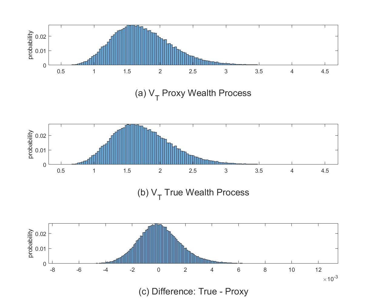
Figure 1: Distribution of terminal wealth for the proxy and exact wealth process

This figure plots the distribution of terminal wealth after a 5-year investment horizon for the approximated wealth process (a) and the exact wealth process (b). Further, it plots the distribution of the difference in terminal wealth after the same horizon in subplot (c).

If an investor wants to follow the optimal wealth process exactly he needs to either pay cash into the strategy or withdraw cash from the strategy in every period i.e. in every period he needs to set $V_{t-1}=\exp(W_{t-1})$. The distribution of the cash flows necessary to maintain such a non-self-financing strategy is shown in Figure 2. The number of simulations for this figure was $100,000$. Subplot (a) displays the distribution of daily cash flows. We observe that the distribution is negatively skewed. This means that in most cases the investor has to supply a small amount of money and in fewer cases he can withdraw a relatively high amount. Most cash flows that need to be supplied to maintain the optimal strategy are in a range from $-0.008\%$ to $0.003\%$ of the investors current wealth. Subplot (b) presents the distribution of the accumulated daily cash flows over the investment horizon of 5 years. It is negatively skewed as well but less so than the distribution in subplot (a). The magnitude of the cumulative cash flows supplied over 5 years is of course somewhat larger than the one of the daily cash flows and lies in a range between $-0.3\%$ and $0.25\%$ of the investors initial wealth. As we will discuss the optimality of our solution for $\gamma\in(0,1]$ later we also performed all calculations for this case. The absolute magnitude of the cash flows was very similar to what is shown here. The distribution seems to be the same but mirrored on a vertical axis at zero i.e. on average cash has to be supplied to the strategy.

Figure 2: Distribution of cash supplied to maintain the optimal wealth process

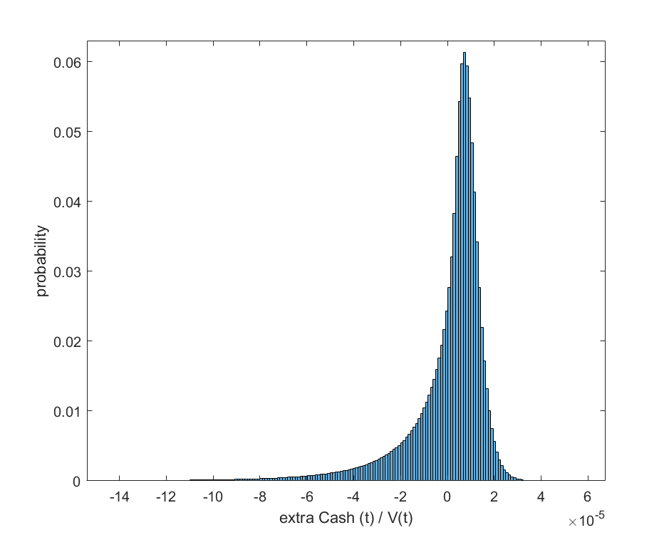
(a) Daily cash flows

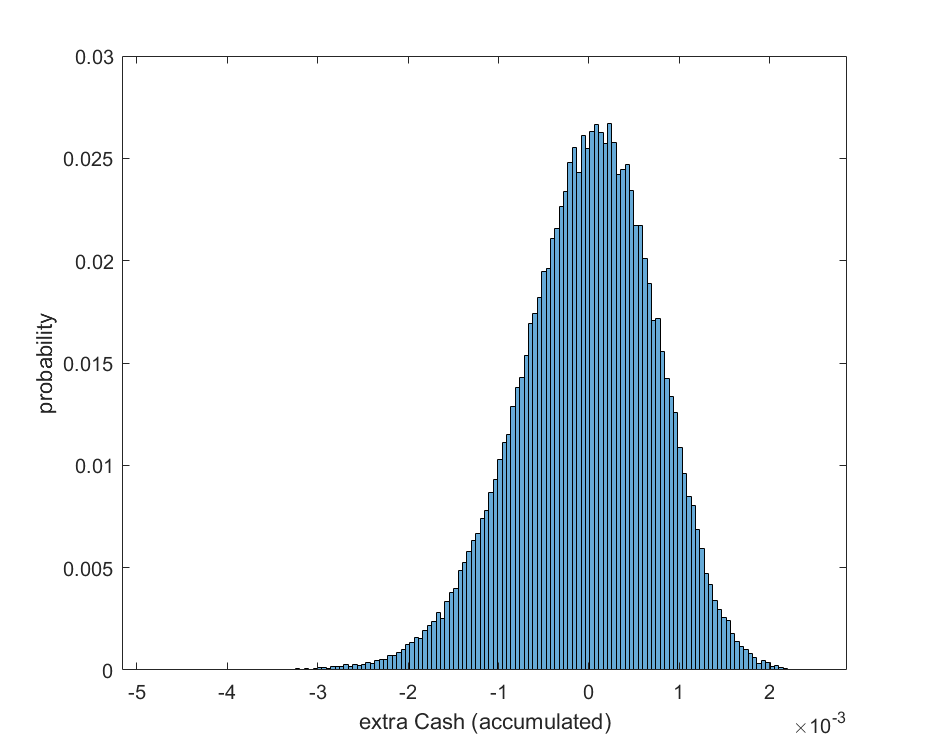
(b) 5-Year cash flows

This figure plots the distribution of the extra cash flows that are necessary to compensate the fact that the approximated wealth process in not exactly self-financing. Subplot (a) displays the distribution of daily cash flows as a fraction of the current wealth. Subplot (b) displays the distribution of the cumulative daily cash flows over a 5-year horizon.

Overall, we conclude that the approximation of the SFC that was used to derive the optimal strategy has only a minor influence on the evolution of the investors wealth.

4.2 Sensitivity of the optimal solution

In this subsection we investigate how the optimal strategy reacts to changes in model parameters. The optimal solution was calculated for $T=252$ trading days and model parameters in a range from 50% to 200% of the estimates in Christoffersen et al., (2006). While varying one parameter all others were held constant to 100% of the Christoffersen et al., (2006) values with $\gamma=-5$. The parameters $\alpha$, $\beta$ and $\theta$ where capped such that the stationarity condition of the HN-GARCH model i.e. $\beta+\alpha\theta^{2}<1$ is satisfied at any time. $\gamma$ was in a range from $-0.1$ to $-10$ and $r$ in the range from $-2\%/252$ to $4\%/252$. The results are shown in Figure 3. The first horizontal axis shows the different values of each parameter, while the second horizontal axis shows the time.

One parameter that stands out is $\lambda$ i.e. the market price of risk. The fraction invested in the risky asset rises linearly with $\lambda$ for all $t$. This is what one would expect. An agent who found a utility maximizing trade-off between risk and reward would not take any more absolute risk unless the reward per unit of additional risk increases. In the latter case, the agent would be willing to invest a higher fraction of wealth in the risky asset. Another obvious picture can be observed for $\gamma$. A lower risk aversion, which corresponds to a $\gamma$ closer to zero, implies a higher investment in the risky asset. $\omega$ and $r$ have no significant impact whatsoever. As for $r$ one can already see from the theoretical results that the optimal strategy is independent of $r$. $\omega$ is traditionally very small when estimating GARCH models and has thus only minor impact on the optimal solution. Often, this parameter is even assumed to be zero.

The more interesting parameters are $\alpha$, $\beta$ and $\theta$. They have a similar impact on the optimal investment as $\pi^{\ast}$ rises with parameters increasing to values that just fulfill the stationarity condition while showing a decreasing sensitivity as $t\longrightarrow T$. $\beta$ is the parameter that models the intensity of autocorrelation in the variance process. Thus, lower values of $\beta$ imply stronger mean-reversion of the variance and vice versa. Furthermore, from (3) we know that lower values of $\beta$ also imply a lower average level of variance. From Figure 3 we can see that it is optimal for an investor to have a higher exposure to the risky asset when $\beta$ is higher i.e. when mean-reversion is weaker and when the average variance is higher. This might seem counter intuitive at first but it becomes clear when digging a little deeper. First, from (1) one can see that if variance increases the expected return increases as well. Thus, for rising values of $\beta$ we have a trade-off between higher variance and higher expected return. Therefore, an increase in $\beta$ does not necessarily imply lower exposure to the risky asset. Second, one has to take correlation into account and note that changes in $\beta$ only impact the non-myopic hedging term. When correlation between stock and variance becomes more negative the hedging effect between the two increases. This is, variance risk and stock risk cancel out to a certain degree. Hence, overall risk decreases and one can invest more risky.

This impact of correlation is consistent with the solution under the Heston model. In the setting of a HN-GARCH model, increasing volatility implies more negative correlation between stock and variance which can be seen from similar considerations as for equation (87). Thus, it makes sense that for some parametric settings an increase in variance increases the non-myopic part of the optimal allocation. Our results show, that this is indeed the case for reasonable model parameters. While in the literature $\alpha$ is mainly held responsible for the kurtosis and $\theta$ for the skewness of multi-period asset returns, both parameters actually influence both distribution characteristics. The increase of each of those parameters leads to an increase in kurtosis and a decrease in skewness i.e. returns become more negatively skewed. It seems intuitive that with decreasing skewness the attractiveness of the risky asset declines. For the kurtosis on the other hand this is not so clear as a higher kurtosis implies a higher probability of both tails of the distribution. Furthermore, as of equation (3) higher values of $\alpha$ or $\theta$ also imply a higher average level of variance and thus more negative correlation between stock and variance. Hence, similar arguments hold as for $\beta$. Our results suggest, that the larger right tail of the returns distribution due to the increase in kurtosis and the more negative correlation between stock and variance lead to an increase in the optimal allocation. Hence, $\pi^{\ast}$ rises with increasing values of $\theta$ and $\alpha$. Furthermore note, that there might be an interdependence of the effect of different parameters on the optimal strategy especially for the parameters $\alpha$, $\beta$ and $\theta$ as they are linked via the stationarity condition. For example, if $\alpha$ is smaller then the impact of the same increase in $\beta$ may be smaller as if $\alpha$ is bigger.

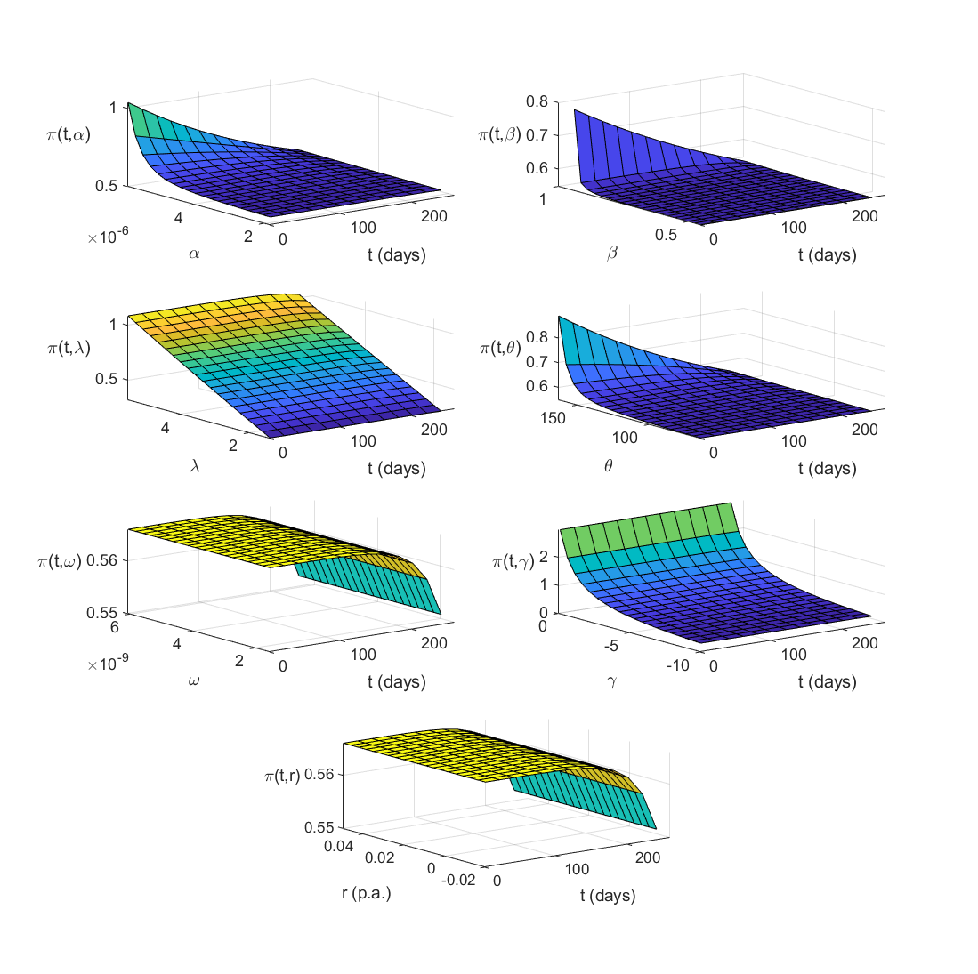
Figure 3: Sensitivity of the optimal solution to various parameters

This figure plots the sensitivity of the optimal investment strategy to changes of various parameters.

Overall we find that the optimal solution is quite robust against small changes in parameters. This is, when parameters are miss-specified, for example due to inaccurate estimation, the resulting strategy is not far off the optimal one using the true parameter set.

4.3 Convergence of the optimal strategy to known solutions

We already related our solution to the continuous-time ones under the Merton and Heston models from a theoretical point of view. Now let’s enrich this with some numerical results.

Figure 4 reports the different portfolio weights over time for the parameter configuration $r=0.01/252$, $T=5\cdot 252$ days. In this figure we denote our solution ”EGZ”. Not surprisingly, given the daily frequency of the parameters, our solution is close to the Heston solution regardless of the sign of $\gamma$. Even though its analytical derivation only shows optimality for $\gamma<0$ explicitly, this fact supports the hypothesis that our solution is optimal for $\gamma<1$, $\gamma\neq 0$ similar to both continuous-time solutions.

Both, the Heston solution and our solution are greater than Merton’s for $\gamma<0$ and smaller than Merton’s for $\gamma>0$ over the whole investment horizon. Overall, all three solutions are rather close to each other for the selected parameter configurations. Note that if $t\longrightarrow T-1$ our solution converges to Merton’s. This is the same result that we found in Section 3.1.

Figure 5 displays the convergence behavior of our solution as $\Delta\longrightarrow 0$. Subplots (a) and (b) show the case where $T=1$ day. We use this investment horizon to show our solution for low rebalancing frequencies, i.e. few rebalancings over the fixed horizon. We have defined the rebalancing frequency as $\frac{T}{\Delta}$ i.e. the number of rebalancing periods over the investment horizon. From Badescu et al., (2019) we know how the parameters change with $\Delta$ for $\Delta\leq 1$ day as we use parameters estimated from daily returns. How the parameters dependent on $\Delta$ for all $\Delta>1$ day for daily returns is unknown in the literature and a topic for future research. Note that, for the purpose of writing our solution dependent on $\Delta$, we need to write the parameter specifications from Badescu et al., (2019) in terms of $h_{t}$ instead of $v_{t}$. As $\Delta$ has this upper bound of $1$, we can only show low rebalancing frequencies $\frac{T}{\Delta}$ by choosing small $T$. Setting $T=1$, $\Delta=0.5$ implies rebalancing twice, $\Delta=0.25$ implies choosing weights four times and so on. For $\Delta<T$ our solution departs from Merton’s and moves towards the Heston solution. The behavior is the same for $\gamma<0$ and $\gamma>0$.

Subplots (c) and (d) in Figure 5 show the convergence behavior for high rebalancing frequencies, i.e. many rebalancing times for the fixed investment horizon. For this we use 5 years i.e. $T=5\cdot 252$ again. In the case $\gamma>0$ (subplot(d)) everything is as suggested by subplot (b). Our solution converges to the Heston solution for $\Delta\longrightarrow 0$. Curiously, subplot (c) which shows the case $\gamma<0$ suggests a ”non-linear” convergence behavior. In most regions of $\Delta$ our solution is smaller than Heston’s and converges to it from below for a shrinking $\Delta$. But for very small rebalancing frequencies, our solution rises above Heston’s before converging back to it from above. This indicates that there are opposite forces at work as $\Delta\longrightarrow 0$, one that pulls our solution towards the Heston solution and one that pushes it above. The, latter seems to dominate only for very specific regions of $\Delta$. An economic explanation for the second force might be that the discrete-time model assumes that there is no movement of the risky asset in-between two points in time, while under the continuous-time model there is movement at any point in time. Thus, the same risky asset might be perceived as less risky under the discrete-time model and therefore a higher stake in the risky asset can be chosen for the same risk preference.

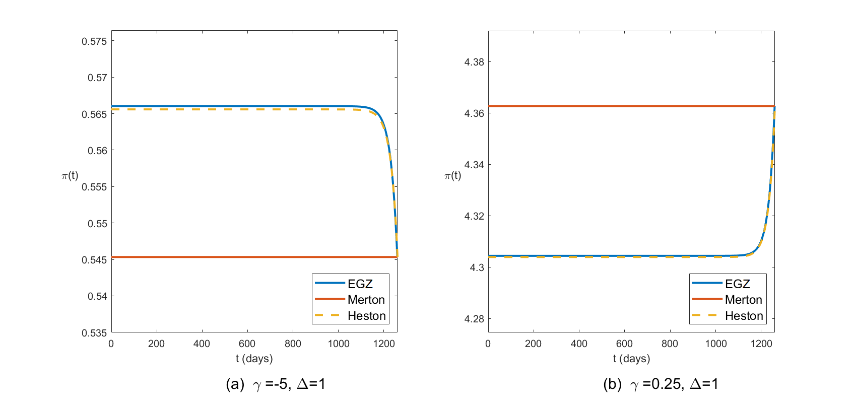
Figure 4: Comparison of different strategies

This figure shows a comparison between our strategy and the Heston and Merton strategy.

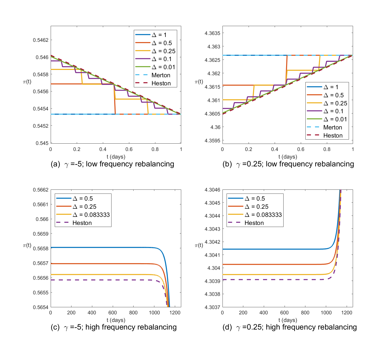
Figure 5: Convergence behavior of the optimal solution

This figure shows convergence behavior of our optimal solution as the time step goes to zero.

4.4 Performance of the optimal and suboptimal strategies

A numerical comparison of the performance for different strategies is conducted in this subsection. We again use simulations to implement some of the analysis. The parameters for the simulation are:

$$V_{0}=1,\quad r=0.01/252,\quad\gamma=-5,\quad T=252\text{ days},\quad\text{number of simulations: }1,000,000$$

Table 1 reports the moments of the one year return distribution and the expected utility from terminal wealth generated by different strategies. The latter was calculated using the closed-form expressions from Theorem 2. The same expressions can also be applied to any other investment strategy as per Lemma 7. We denote our optimal strategy ”EGZ”. ”Heston” refers to the strategy from Kraft, (2005) while ”Merton” refers to the one from Merton, (1969). Merton’s strategy deviates the most from the other two. We can see that it produces a slightly higher Sharpe ratio and lower kurtosis than the other two strategies. On the other hand it also has more negatively skewed returns and most importantly it obviously has a lower expected utility from terminal wealth. The Heston solution holds up quite well in our setting based on this analysis.

strategy	$\mu$	$\sigma$	skewness	kurtosis	SR	$E[U_{T}]$
EGZ	0.0567	0.0863	-0.1472	3.0546	0.6568	-168.9989E-03
Heston	0.0566	0.0863	-0.1471	3.0471	0.6560	-168.9990E-03
Merton	0.0552	0.0833	-0.1561	3.0494	0.6628	-169.0227E-03

Table 1: Distribution moments of realized returns and expected utility from terminal wealth generated by different strategies.

Based on the results from Section 3.3, we further estimate the utility loss for an investor who follows a suboptimal strategy. We start by exploring the WEL induced by following the Heston and the Merton strategy instead of the strategy optimal to this setting and its sensitivity towards the risk aversion parameter $\gamma$. The results are shown in Figure 6. Subplot (a) shows the whole region, while subplot (b) provides a closer look at the comparison to the Heston strategy. The first thing to note is that, for the parameter set at hand, WEL is relatively small over all values of $\gamma$. Furthermore, the WEL induced by the Heston solution is almost negligible compared to the one induced by Merton’s solution.

Figure 6: Wealth-equivalent loss from suboptimal strategies with $T=252*10$ days.

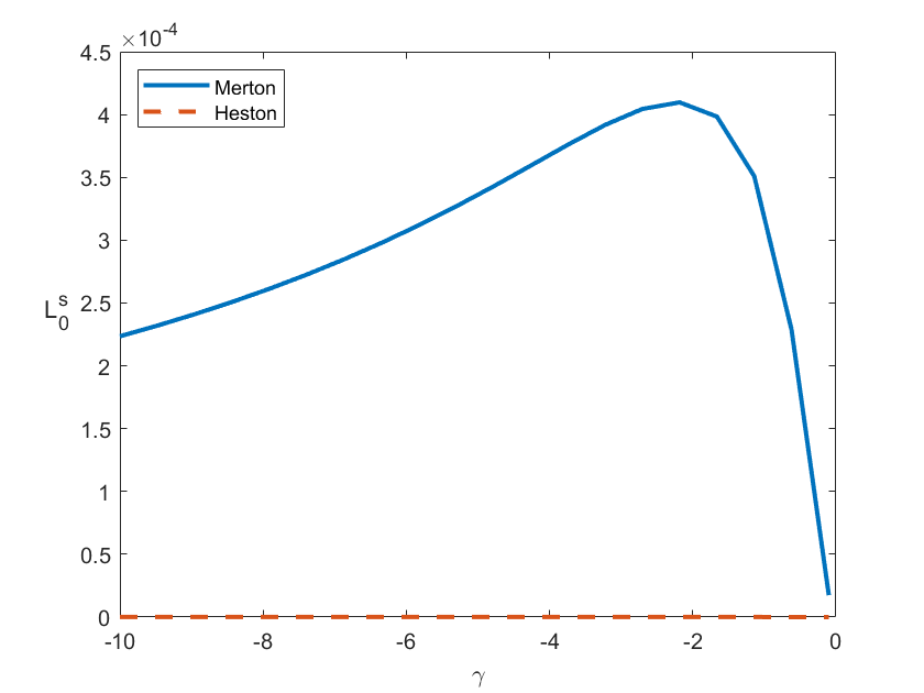
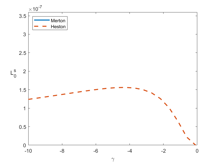
This figure plots the WEL induced by following Merton’s and Heston’s strategy for different levels of risk aversion $\gamma$. Subplot (a) shows the whole picture, subplot (b) provides a closer look at the comparison to the Heston strategy.

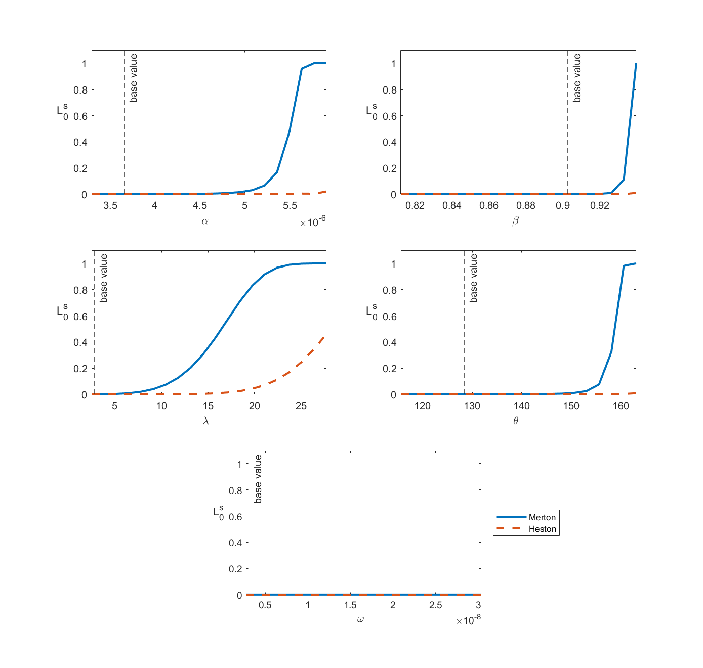
Figure 7: Wealth-equivalent loss from following suboptimal strategies with $T=252\cdot 10$ days and $\gamma=-5$.

This figure plots the WEL induced by following Merton’s and Heston’s strategy for different parameter configurations.

In Figure 7 we report the WEL when exploring other reasonable values for each parameter while keeping all other parameters unchanged. When varying the parameters we ensure that the stationarity condition as well as the technical condition $1-2\alpha E_{t,T}^{s}>0$ from Section 3.3 are satisfied. Other parameter regions than the ones shown in the plots do not reveal any additional insights.

Recall, the WEL is calculated via the formula in Lemma 8. For the purpose of these numerical examples we set $h_{t+1}=h$ using the original parameters from Christoffersen et al., (2006). This gives us an annualized volatility at time $t+1$ of $0.1578$ which is not modified along with the model parameters. The reason for this is that if we recalculate $h_{t+1}$ using the varied parameters, $h_{t+1}$ would inflate as $\alpha$, $\beta$ or $\theta$ approach values that only just fulfill the stationarity condition. This would cause the WEL to explode, i.e. $exp()$ in Lemma 8 goes to $-\infty$ due to $\gamma<0$. However, we are interested in the WEL that is induced by the difference in the strategies i.e. $D_{t,T}^{s}-D_{t,T}$ and/or $E_{t,T}^{s}-E_{t,T}^{\ast}$ and not by the inflation of $h_{t+1}$. Keeping $h_{t+1}$ unchanged implies that Figure 7 can answer the following question. If we observe an annualized variance of $0.1578$ today, what would be the impact of changing one model parameter on the WEL?

We observe that WEL rises as the values of $\alpha$, $\beta$, $\theta$ or $\lambda$ increase. For the first three parameters, the loss inferred by following the Heston strategy is negligible, the one inferred by Merton’s solution on the other hand rises significantly. This behavior is reasonable because if these parameters rise, then the variance becomes more random hence creating a larger separation to Merton. The Merton solution completely disregards the fact that variance is random in the HN-GARCH setting. Explicitly modeling the variance gives additional information about how the variance moves that can be exploited to achieve a higher expected utility or more precisely the highest possible expected utility. $\omega$ has almost no impact on WEL whatsoever because the optimal strategy is not sensitive to changes in $\omega$ as demonstrated in Section 4.2. $\lambda$ i.e. the equity risk premium has a significant impact on WEL. Recall from Figure 3, that $\lambda$ already had a significant impact on the overall strategy. However, from representation (27) one can see that it not only plays a role in the myopic but also in the non-myopic part of the strategy. As its influence on the myopic part is the same as for Merton’s strategy one can follow from Figure 7 that the non-myopic part becomes more and more important for larger values of $\lambda$. Economically, the WEL induced by following Merton’s strategy can be explained as follows. $\lambda$ is the risk premium per unit of variance. Merton assumes a constant variance that means the premium ($\lambda h_{t}$) he can collect is always the same. If one knows how variance moves over time, one can better incorporate how the premium ($\lambda h_{t}$) moves over time and thus collect this premium better. When looking at the Heston strategy, one can see that $\lambda$ also has the biggest impact on WEL. As the only difference between the Heston strategy and ours is the size of one period this has to be the reason for the WEL induced by following the Heston strategy. A possible economic interpretation is that Heston over- or underestimates the opportunity to exploit the risk premium by assuming the risky asset moves continuously while it actually does only move at certain points in time. Furthermore, it is likely that WEL significantly increases when using larger rebalancing frequencies.

In summary, WEL induced by following either Merton’s or the Heston solution instead of ours is rather small within this parameter set. However, there are reasonable regions of parameters where WEL increases to a considerable level.

5 Conclusion

This paper develops a closed-form solution for a portfolio optimization problem where the investor maximizes a CRRA utility from terminal wealth assuming that the variance of the spot asset follows the HN-GARCH model. To avoid the possibility of a negative wealth we employ an approximation for the wealth process.

In our two-asset setting, we find that the optimal portfolio process is independent of the development of the risky asset and non-myopic i.e. has a time-dependent component. In the limit where the length of one period goes to zero our solution converges to the one under the Heston stochastic volatility model under some conditions. Further we obtain a recursive representation for the conditional m.g.f. of the optimal (and any other) wealth process facilitating risk management and pricing.

Finally, using empirically relevant parameter estimates, we conduct a numerical analysis of our optimal strategy. Firstly, we find that the approximation of the wealth process has only minor impact. Secondly, our strategy is quite robust against changes in parameter values. Thirdly, we visualize the connection between our solution, the one under the Heston model and the one under the Merton model. Our strategy contains both of the other strategies as a special case i.e. the case $\Delta\longrightarrow 0$ and the case $\Delta=T$. And lastly, we investigate the WEL induced by following the Heston and the Merton strategy for different parameter settings. We report that, for a daily trading scenario, the optimal solution under the Heston model shows a good performance while the optimal solution under the Merton model shows significant losses.

Overall, this paper provides a quick method of finding utility-optimal portfolios under an advanced time-series model which is easy to implement and takes into account important stylized facts.

Appendix A Proofs

Proof of Theorem 2. We prove the statements (21)-(25) from Theorem 2 by induction.
Base case We start by optimizing the last period first i.e. from $T-1$ to $T$ and use this as the base case. Let us solve problem (12) backward using Bellman’s principle. The first step reads

$$\Phi_{T-1}(W_{T-1},h_{T})=\underset{\pi_{T-1}}{\max}\mathbb{E}_{T-1}\left[\frac{\exp\left\{\gamma W_{T}\right\}}{\gamma}\right]$$

where from (10) we have $W_{T}=W_{T-1}+r+\left(\pi_{T-1}-\pi_{T-1}^{2}\right)\frac{1}{2}h_{T}+\pi_{T-1}\left(\lambda h_{T}+\sqrt{h_{T}}z_{T}\right)$.
From Heston and Nandi, (2000) we know the one-period m.g.f. of the log stock under the HN-GARCH model $\Psi_{X_{t}}^{\left(t-1\right)}$ is

$$\Psi_{X_{T}}^{\left(T-1\right)}\left(u\right) =\mathbb{E}_{T-1}[e^{uX_{T}}]=\exp\left(uX_{T-1}+A_{T-1,T}+B_{T-1,T}h_{T}\right)$$

$$A_{T-1,T} =ur,\quad B_{T-1,T}=u\lambda+\dfrac{1}{2}u^{2}.$$

Using this we can produce the m.g.f. for log wealth as

$$\Psi_{W_{t}}^{\left(t-1\right)}\left(u\right) =\mathbb{E}_{t-1}\left[\exp\left\{uW_{t}\right\}\right]$$

$$=\Psi_{X_{t}}^{\left(t-1\right)}\left(u\pi_{t-1}\right)\times\exp\left\{u\left(W_{t-1}-\pi_{t-1}X_{t-1}+\left(\pi_{t-1}-\pi_{t-1}^{2}\right)\frac{1}{2}h_{t}+\left(1-\pi_{t-1}\right)r\right)\right\}$$

$$=\exp\left\{uW_{t-1}+ur+\left(\pi_{t-1}u\lambda+\pi_{t-1}^{2}\dfrac{1}{2}u^{2}+\left(\pi_{t-1}-\pi_{t-1}^{2}\right)u\frac{1}{2}\right)h_{t}\right\}$$ (50)

Note this is the exponential of a polynomial of order two on $\pi_{t-1}$, which will be used to maximize on $\pi_{t-1}$. With this we can rewrite the problem as

$$\Phi_{T-1}(W_{T-1},h_{T})=\underset{\pi_{T-1}}{\max}\mathbb{E}_{T-1}\left[\frac{\exp\left\{\gamma W_{T}\right\}}{\gamma}\right]=\underset{\pi_{T-1}}{\max}\frac{1}{\gamma}\Psi_{W_{T}}^{\left(T-1\right)}\left(\gamma\right)$$

=π_T-1max1γexp{γW_T-1+γr +(π_T-1γλ+π_T-1^212γ^2+γ(π_T-1-π_T-1^2)12) h_T}

$$=\underset{\pi_{T-1}}{\max}\frac{1}{\gamma}\exp\left\{D_{T-1,T}+\gamma W_{T-1}+E_{T-1,T}(\pi_{T-1})h_{T}\right\}$$ (51)

where $D_{T-1,T}=\gamma r,\quad E_{T-1,T}(\pi_{T-1})=\pi_{T-1}\left(\lambda+\frac{1}{2}\right)\gamma+\pi_{T-1}^{2}\dfrac{1}{2}\left(\gamma^{2}-\gamma\right)$. Before carrying on, note that in (51) only $E_{T-1,T}(\pi_{T-1})$ depends on $\pi_{T-1}$ and that the exponential function is strictly monotonously increasing in $E_{T-1,T}(\pi_{T-1})$. Therefore, it is sufficient to only optimize $E_{T-1,T}(\pi_{T-1})$. Further, note that the sign of the second derivative of the overall optimization problem is only depending on the signs of $\gamma$ and $E_{T-1,T}^{\prime\prime}$. Therefore, it is also sufficient to calculate $E_{T-1,T}^{\prime\prime}$. With this we can proceed to solve the optimization problem in (51) by taking the first derivative of $E_{T-1,T}(\pi_{T-1})$ w.r.t. $\pi_{T-1}$ and set it equal to zero,

$$\left(\lambda+\frac{1}{2}\right)\gamma+\pi_{T-1}^{\ast}\left(\gamma^{2}-\gamma\right)=0\Leftrightarrow\pi_{T-1}^{\ast}=\frac{\lambda+\frac{1}{2}}{1-\gamma}.$$ (52)

To check whether this is a minimum or a maximum we calculate the second derivative of $E_{T-1,T}(\pi_{T-1})$ as $\gamma^{2}-\gamma>0,\quad\gamma<0.$ This shows that the optimum from above is maximizing if $\gamma<0$. However, one can not be sure that the solution is minimizing for $\gamma>0$. Substituting $\pi^{\ast}_{T-1}$ into equation (51) leads to

$$\Phi_{T-1}(W_{T-1},h_{T}) =\frac{1}{\gamma}\exp\left\{D_{T-1,T}+\gamma W_{T-1}+E_{T-1,T}^{\ast}h_{T}\right\}$$ (53)

$$=\frac{1}{\gamma}\exp\left\{\gamma r+\gamma W_{T-1}+\frac{\gamma(\lambda+\frac{1}{2})^{2}}{2(1-\gamma)}h_{T}\right\}$$ (54)

where $E_{T-1,T}^{\ast}=E_{T-1,T}(\pi_{T-1}^{\ast})=(\lambda+\frac{1}{2})^{2}\left(\frac{\gamma}{1-\gamma}+\frac{1}{2}\frac{1}{(1-\gamma)^{2}}(\gamma^{2}-\gamma)\right)=\frac{\gamma(\lambda+\frac{1}{2})^{2}}{2(1-\gamma)}$. Hence, $\Phi_{T-1}\in\mathbb{M}$. We can rewrite the terminal condition (18) as

$$\Phi_{T}(W_{T},h_{T+1})=\Phi_{T}(W_{T})=\frac{\exp\left\{\gamma W_{T}\right\}}{\gamma}\in\mathbb{M}.$$ (55)

This in combination with equation (53) imposes terminal conditions on $D_{t,T}$ and $E_{t,T}^{\ast}$: $D_{T,T}=0$, and $E_{T,T}^{\ast}=0$.

Inductive step Next we will perform the inductive step by assuming that the statements hold for a particular $t+1$ and showing that in this case they also hold for $t$. Moving one step backward from $t+1$ to $t$ by applying Bellman’s principle like before we get after plugging in the definitions of $W_{t+1}$ and $h_{t+2}$ and some algebraic manipulation:

$$\Phi_{t}(W_{t},h_{t+1})=\underset{\pi_{t}}{\max}\mathbb{E}_{t}\left[\Phi_{t+1}(W_{t+1},h_{t+2})\right]=\underset{\pi_{t}}{\max}\mathbb{E}_{t}\left[\frac{1}{\gamma}\exp\left\{D_{t+1,T}+\gamma W_{t+1}+E_{t+1,T}^{\ast}h_{t+2}\right\}\right]$$

$$=\underset{\pi_{t}}{\max}\left\{\begin{array}[]{c}\frac{1}{\gamma}\exp(D_{t+1,T}+\gamma\left(W_{t}+r+\pi_{t}\lambda h_{t+1}+\left(\pi_{t}-\pi_{t}^{2}\right)\frac{1}{2}h_{t+1}\right)\\ +E_{t+1,T}^{\ast}\left(\omega+\beta h_{t+1}+\alpha\theta^{2}h_{t+1}\right))\\ \times\mathbb{E}_{t}\left[\exp\left\{\left(\gamma\pi_{t}-2E_{t+1,T}^{\ast}\alpha\theta\right)\sqrt{h_{t+1}}z_{t+1}+E_{t+1,T}^{\ast}\alpha z_{t+1}^{2}\right\}\right]\end{array}\right\}$$

A useful result for a standard normal variable $z$ is that, like in Heston and Nandi, (2000),

$$\mathbb{E}[\exp(aX^{2}+bX)] =\dfrac{1}{\sqrt{(1-2a)}}\exp\left(\dfrac{b^{2}}{2(1-2a)}\right).$$ (56)

With this we reduce the expectation to

$$\mathbb{E}_{t}\left[\exp\left\{\left(\gamma\pi_{t}-2E_{t+1,T}^{\ast}\alpha\theta\right)\sqrt{h_{t+1}}z_{t+1}+E_{t+1,T}^{\ast}\alpha z_{t+1}^{2}\right\}\right]$$

$$=\dfrac{1}{\sqrt{1-2E_{t+1,T}^{\ast}\alpha}}\exp\left(\dfrac{\left(\gamma\pi_{t}-2E_{t+1,T}^{\ast}\alpha\theta\right)^{2}}{2(1-2E_{t+1,T}^{\ast}\alpha)}h_{t+1}\right).$$

Here we need $1-2\alpha E_{t,T}^{\ast}>0$ for the solution to be well defined, again. Plugging this in and grouping yields

$$\Phi_{t}(W_{t},h_{t+1}) =\underset{\pi_{t}}{\max}\dfrac{1}{\gamma\sqrt{1-2E_{t+1,T}^{\ast}\alpha}}$$

$$\times\exp\left\{\begin{array}[]{c}D_{t+1,T}+\gamma\left(W_{t}+r\right)+E_{t+1,T}^{\ast}\omega\\ +\left(\gamma\left(\lambda+\frac{1}{2}\right)\pi_{t}-\gamma\frac{1}{2}\pi_{t}^{2}+E_{t+1,T}^{\ast}\left(\beta+\alpha\theta^{2}\right)+\dfrac{\left(\gamma\pi_{t}-2E_{t+1,T}^{\ast}\alpha\theta\right)^{2}}{2(1-2E_{t+1,T}^{\ast}\alpha)}\right)h_{t+1}\end{array}\right\}$$ (59)

$$=\underset{\pi_{t}}{\max}\frac{1}{\gamma}\exp\left\{D_{t,T}+\gamma W_{t}+E_{t,T}(\pi_{t})h_{t+1}\right\}$$ (60)

where

$$D_{t,T} =E_{t+1,T}^{\ast}\omega+\gamma r+D_{t+1,T}-\log\left(\sqrt{(1-2\alpha E_{t+1,T}^{\ast})}\right)$$ (61)

$$E_{t,T}(\pi_{t}) =\left(\beta+\alpha\theta^{2}\right)E_{t+1,T}^{\ast}+\dfrac{\left(\gamma\pi_{t}-2\theta\alpha E_{t+1,T}^{\ast}\right)^{2}}{2(1-2\alpha E_{t+1,T}^{\ast})}+\gamma\left(\left(\lambda+\frac{1}{2}\right)\pi_{t}-\frac{1}{2}\pi_{t}^{2}\right).$$ (62)

Solving the optimization problem in (60) yields

$$\frac{1}{2(1-2\alpha E_{t+1,T}^{\ast})}\left(\gamma^{2}2\pi_{t}^{\ast}-4\gamma E_{t+1,T}^{\ast}\alpha\theta\right)-\gamma\pi_{t}^{\ast}+\gamma\left(\lambda+\frac{1}{2}\right)=0$$

$$\Leftrightarrow\pi_{t}^{\ast} =\left(\frac{2\gamma E_{t+1,T}^{\ast}\alpha\theta-\gamma\left(\lambda+\frac{1}{2}\right)(1-2\alpha E_{t+1,T}^{\ast})}{1-2\alpha E_{t+1,T}^{\ast}}\right)\left(\frac{1-2\alpha E_{t+1,T}^{\ast}}{\gamma^{2}-\gamma(1-2\alpha E_{t+1,T}^{\ast})}\right)$$

$$=\frac{\lambda+\frac{1}{2}}{(1-2\alpha E_{t+1,T}^{\ast})-\gamma}-\frac{\left(\theta+(\lambda+\frac{1}{2})\right)2\alpha E_{t+1,T}^{\ast}}{(1-2\alpha E_{t+1,T}^{\ast})-\gamma}.$$ (63)

To check whether this is a minimum or a maximum we calculate the second derivative of $E_{t,T}(\pi_{t})$ as $\frac{1}{\underbrace{1-2\alpha E_{t+1,T}^{\ast}}_{>0}}\underbrace{\gamma^{2}}_{>0}\underbrace{-\gamma}_{>0}>0,\quad\gamma<0$. Therefore, one can see that the assumption $\gamma<0$ is sufficient but not necessary for any general $t$. If $\gamma>0$, we can not be sure that it is minimizing. Plugging $\pi_{t}^{\ast}$ into equation (60) yields $\Phi_{t}(W_{t},h_{t+1})=\frac{1}{\gamma}\exp\left\{D_{t,T}+\gamma W_{t}+E_{t,T}^{\ast}h_{t+1}\right\}$ where in terms of $E^{\ast}_{t+1,T}$

$$E_{t,T}^{\ast}=\left(\beta+\alpha\theta^{2}\right)E_{t+1,T}^{\ast}+\dfrac{\left(\gamma\pi_{t}^{\ast}-2\theta\alpha E_{t+1,T}^{\ast}\right)^{2}}{2(1-2\alpha E_{t+1,T}^{\ast})}+\gamma\left((\lambda+\frac{1}{2})\pi_{t}^{\ast}-\frac{1}{2}(\pi_{t}^{\ast})^{2}\right).$$ (64)

Hence, $\Phi_{t}\in\mathbb{M}$. Starting from the induction hypothesis that the statement holds for $t+1$ we have shown that in this case it also holds for $t$.

Proof of (26) as representation of $W_{t}^{\ast}$. We conjecture that the analytical expression of $W_{t}^{\ast}$ is given by Equation 26. We will prove it by induction. The Base case is straight forward to see that if we plug $t=1$ into the conjecture, we recover (28) which is the definition of $W_{t}^{\ast}$. Thus, the statement holds for the base case.
Inductive step: The induction hypothesis is that Equation 26 holds for a particular $t$. It follows by adding $\left((\lambda+\frac{1}{2})\pi_{t}^{\ast}-\frac{1}{2}(\pi_{t}^{\ast})^{2}\right)h_{t+1}+\pi_{t}^{\ast}\sqrt{h_{t+1}}z_{t+1}+r$ on both sides of the equation that

$$W^{\ast}_{t}+\left((\lambda+\frac{1}{2})\pi_{t}^{\ast}-\frac{1}{2}(\pi_{t}^{\ast})^{2}\right)h_{t+1}+\pi_{t}^{\ast}\sqrt{h_{t+1}}z_{t+1}+r$$

$$=w_{0}+\sum_{k=1}^{t}\left((\lambda+\frac{1}{2})\pi_{t-k}^{\ast}-\frac{1}{2}(\pi_{t-k}^{\ast})^{2}\right)h_{t+1-k}+\sum_{k=1}^{t}\left(\pi_{t-k}^{\ast}\sqrt{h_{t+1-k}}z_{t+1-k}\right)+rt$$

$$+\left((\lambda+\frac{1}{2})\pi_{t}^{\ast}-\frac{1}{2}(\pi_{t}^{\ast})^{2}\right)h_{t+1}+\pi_{t}^{\ast}\sqrt{h_{t+1}}z_{t+1}+r.$$

By (28) the left-hand side of this equation is equal to $W_{t+1}^{\ast}$. The right-hand side can be written as

$$w_{0}+\sum_{k=1}^{t+1}\left((\lambda+\frac{1}{2})\pi_{t+1-k}^{\ast}-\frac{1}{2}(\pi_{t+1-k}^{\ast})^{2}\right)h_{(t+1)+1-k}+\sum_{k=1}^{t+1}\left(\pi_{t+1-k}^{\ast}\sqrt{h_{(t+1)+1-k}}z_{(t+1)+1-k}\right)+r(t+1).$$

Equating both sides, we deduce the statement also holds true for $t+1$.

Appendix B Complementary material

Proof of Lemma 1 Using (2) we can write

$$\mathbb{E}[h_{t}] =\alpha+\omega+(\beta+\alpha\theta^{2})\mathbb{E}[h_{t-1}].$$ (65)

This we can use as a starting point and plug in the analogue expressions for $\mathbb{E}[h_{t-1}],\mathbb{E}[h_{t-2}],\dots,\mathbb{E}[h_{0}]$. From this we conjecture that the analytical representation is given by

$$\mathbb{E}[h_{t}] =\left(\alpha+\omega\right)\sum_{i=0}^{t-1}\left((\beta+\alpha\theta^{2})^{i}\right)+(\beta+\alpha\theta^{2})^{t}h_{0}.$$ (66)

Now that we have a guess for the analytical expression of $\mathbb{E}[h_{t}]$, we will prove it by induction next.

Base case:
We use $t=1$ as a base case which is true by (65).

Inductive step:
The induction hypothesis is that (66) holds for a particular $t$. It follows by multiplying by $\left(\beta+\alpha\theta^{2}\right)$ and adding $(\alpha+\omega)$ on both sides of the equation that

$$\mathbb{E}[h_{t}]\left(\beta+\alpha\theta^{2}\right)+\alpha+\omega=\left[\left(\alpha+\omega\right)\sum_{i=0}^{t-1}\left((\beta+\alpha\theta^{2})^{i}\right)+(\beta+\alpha\theta^{2})^{t}h_{0}\right]\left(\beta+\alpha\theta^{2}\right)+\alpha+\omega.$$

By (65) the left-hand side of this equation is equal to $\mathbb{E}[h_{t+1}]$. The right-hand side can be written as

$$\left(\alpha+\omega\right)\left[1+\sum_{i=1}^{t}\left((\beta+\alpha\theta^{2})^{i}\right)\right]+(\beta+\alpha\theta^{2})^{t+1}h_{0}=\left(\alpha+\omega\right)\sum_{i=0}^{t}\left((\beta+\alpha\theta^{2})^{i}\right)+(\beta+\alpha\theta^{2})^{t+1}h_{0}.$$

Equating both sides, we deduce the statement for $t+1$, establishing the inductive step.

Conclusion:
Since both the base case and the inductive step have been proved as true, by mathematical induction statement (66) holds for every $t$.

Up to this point we have proven that statement (66) is true. By observing that the first part of this representation is a geometric series we can get

$$\mathbb{E}[h_{t}]=\left(\alpha+\omega\right)\left(\frac{1-\left(\beta+\alpha\theta^{2}\right)^{t}}{1-\left(\beta+\alpha\theta^{2}\right)}\right)+(\beta+\alpha\theta^{2})^{t}h_{0}.$$ (67)

Proof of Corollary 4. The proof of the fact that the process is a GARCH model of the Heston-Nandi type is straight forward. Knowing that $\left\{\pi_{t}^{\ast}\right\}_{t\in\left\{0,1,\dots,T\right\}}$ is deterministic one can see that (28) has the exact same form as the HN-GARCH model.
Proof of conditional recursive m.g.f.
Step 1: We first compute the one-period moment generating function of $W_{t+1}^{\ast}$,

$$\mathbb{E}[e^{uW_{t+1}^{\ast}}\mid\mathcal{F}_{t}]$$=E[exp(uW_t^∗ + u((λ+12)π_t^∗-12(π_t^∗)^2)h_t+1 + uπ_t^∗h_t+1z_t+1 + ur) ∣F_t]

$$=\exp\left(uW_{t}^{\ast}+u\left((\lambda+\frac{1}{2})\pi_{t}^{\ast}-\frac{1}{2}(\pi_{t}^{\ast})^{2}\right)h_{t+1}+ur\right)\mathbb{E}[e^{u\pi_{t}^{\ast}\sqrt{h_{t+1}}z_{t+1}}\mid\mathcal{F}_{t}]$$

=exp( uW_t^∗ + u((λ+12)π_t^∗-12(π_t^∗)^2)h_t+1 + ur) exp(0+12u^2(π_t^∗)^2h_t+1)

$$=\exp\left(uW_{t}^{\ast}+A_{t,t+1}+B_{t,t+1}h_{t+1}\right)$$ (68)

with $A_{t,t+1}$ and $B_{t,t+1}$ given by

$$A_{t,t+1} =ur,\quad B_{t,t+1}=u\left((\lambda+\frac{1}{2})\pi_{t}^{\ast}-\frac{1}{2}(\pi_{t}^{\ast})^{2}\right)+\dfrac{1}{2}u^{2}\left(\pi_{t}^{\ast}\right)^{2}$$ (69)

Step 2: We now compute the two-periods m.g.f of $W_{t+2}^{\ast}$ using the tower rule of expectations

$$\mathbb{E}[e^{uW_{t+2}^{\ast}}\mid\mathcal{F}_{t}]=\mathbb{E}[\mathbb{E}[e^{uW_{t+2}^{\ast}}\mid\mathcal{F}_{t+1}]\mid\mathcal{F}_{t}].$$

Let us move outward with the inner expectations. Using equations (B) and (69) we get

$$\mathbb{E}[e^{uW_{t+2}^{\ast}} \mid\mathcal{F}_{t+1}]=\exp\left(uW_{t+1}^{\ast}+A_{t+1,t+2}+B_{t+1,t+2}h_{t+2}\right)$$

$$A_{t+1,t+2} =ur,\quad B_{t+1,t+2}=u\left((\lambda+\frac{1}{2})\pi_{t+1}^{\ast}-\frac{1}{2}(\pi_{t+1}^{\ast})^{2}\right)+\dfrac{1}{2}u^{2}\left(\pi_{t+1}^{\ast}\right)^{2}.$$

Next,

$$\mathbb{E}[e^{uW_{t+2}^{\ast}}\mid\mathcal{F}_{t}]$$

$$=\mathbb{E}[\mathbb{E}[e^{uW_{t+2}^{\ast}}\mid\mathcal{F}_{t+1}]\mid\mathcal{F}_{t}]$$

$$=\mathbb{E}[\exp\left(uW_{t+1}^{\ast}+A_{t+1,t+2}+B_{t+1,t+2}h_{t+2}\right)\mid\mathcal{F}_{t}]$$

$$=\mathbb{E}\left[\exp\left(\begin{array}[]{c}u\left(W_{t}^{\ast}+\left((\lambda+\frac{1}{2})\pi_{t}^{\ast}-\frac{1}{2}(\pi_{t}^{\ast})^{2}\right)h_{t+1}+\pi_{t}^{\ast}\sqrt{h_{t+1}}z_{t+1}+r\right)+A_{t+1,t+2}\\ +B_{t+1,t+2}\left(\omega+\beta h_{t+1}+\alpha\left(z_{t+1}-\theta\sqrt{h_{t+1}}\right)^{2}\right)\end{array}\right)\mid\mathcal{F}_{t}\right]$$

$$=\exp\left(\begin{array}[]{c}uW_{t}^{\ast}+u\left((\lambda+\frac{1}{2})\pi_{t}^{\ast}-\frac{1}{2}(\pi_{t}^{\ast})^{2}\right)h_{t+1}+ur+A_{t+1,t+2}\\ +\omega B_{t+1,t+2}+B_{t+1,t+2}\beta h_{t+1}+B_{t+1,t+2}\alpha\theta^{2}h_{t+1}\end{array}\right)$$

$$\times\mathbb{E}\left[\exp\left(B_{t+1,t+2}\alpha z_{t+1}^{2}+z_{t+1}\left(u\pi_{t}^{\ast}\sqrt{h_{t+1}}-2\theta\sqrt{h_{t+1}}B_{t+1,t+2}\alpha\right)\right)\mid\mathcal{F}_{t}\right]$$

To proceed, we use(56) to calculate the expectation. This gives

$$\mathbb{E}[e^{uW_{t+2}^{\ast}}\mid\mathcal{F}_{t}]$$

$$=\exp\left(\begin{array}[]{c}uW_{t}^{\ast}+u\left((\lambda+\frac{1}{2})\pi_{t}^{\ast}-\frac{1}{2}(\pi_{t}^{\ast})^{2}\right)h_{t+1}+ur+A_{t+1,t+2}\\ +\omega B_{t+1,t+2}+B_{t+1,t+2}\beta h_{t+1}+B_{t+1,t+2}\alpha\theta^{2}h_{t+1}\end{array}\right)$$ (72)

$$\times\exp\left(-\dfrac{1}{2}\log(1-2B_{t+1,t+2}\alpha)+\dfrac{\left(u\pi_{t}^{\ast}\sqrt{h_{t+1}}-2\theta\sqrt{h_{t+1}}B_{t+1,t+2}\alpha\right)^{2}}{2(1-2B_{t+1,t+2}\alpha)}\right)$$

$$=\exp\left(uW_{t}^{\ast}+A_{t,t+2}+B_{t,t+2}h_{t+1}\right)$$ (73)

with $A_{t,t+2},B_{t,t+2}$ given by

$$A_{t,t+2} =ur+A_{t+1,t+2}+\omega B_{t+1,t+2}-\dfrac{1}{2}\log(1-2B_{t+1,t+2}\alpha)$$ (74)

$$B_{t,t+2} =u\left((\lambda+\frac{1}{2})\pi_{t}^{\ast}-\frac{1}{2}(\pi_{t}^{\ast})^{2}\right)+B_{t+1,t+2}\left(\beta+\alpha\theta^{2}\right)+\dfrac{\left(u\pi_{t}^{\ast}-2\theta B_{t+1,t+2}\alpha\right)^{2}}{2(1-2B_{t+1,t+2}\alpha)}$$ (75)

$$A_{t+1,t+2} =ur,\quad$$ (76)

$$B_{t+1,t+2} =u\left((\lambda+\frac{1}{2})\pi_{t+1}^{\ast}-\frac{1}{2}(\pi_{t+1}^{\ast})^{2}\right)+\dfrac{1}{2}u^{2}\left(\pi_{t+1}^{\ast}\right)^{2}$$ (77)

So we obtain the m.g.f of $W_{t+2}^{\ast}$ as

$$\mathbb{E}[e^{uW_{t+2}^{\ast}}\mid\mathcal{F}_{t}]=\exp\left(uW_{t}^{\ast}+A_{t,t+2}+B_{t,t+2}h_{t+1}\right).$$

Observe that $A_{t,t+2},B_{t,t+2}$ are functions of $A_{t+1,t+2},B_{t+1,t+2}$ and $u$. Continuing recursively we can find the m.g.f of $W_{T}^{\ast}$ as

$$\mathbb{E}_{t}[e^{uW_{T}^{\ast}}] =\exp\left(uW_{t}^{\ast}+A_{t,T}+B_{t,T}h_{t+1}\right)$$

$$A_{t,T} =A_{t+1,T}+ur+B_{t+1,T}\omega-\dfrac{1}{2}\log(1-2\alpha B_{t+1,T}),\quad t=0,\dots,T-1$$

$$B_{t,T} =u\left((\lambda+\frac{1}{2})\pi_{t}^{\ast}-\frac{1}{2}(\pi_{t}^{\ast})^{2}\right)+\left(\beta+\alpha\theta^{2}\right)B_{t+1,T}+\dfrac{(u\pi_{t}^{\ast}-2\alpha\theta B_{t+1,T})^{2}}{2(1-2\alpha B_{t+1,T}\,)},\quad t=0,\dots,T-1$$

$$A_{T,T} =B_{T,T}=0.$$

Proof of Corollary 5. This follows by virtue of Theorem 2 combined with the formula for the multi-period expectation of $h_{t}$ from Lemma 1 yielding

$$\mathbb{E}_{0}[W_{t}^{\ast}]=w_{0}+rt$$

$$+\sum_{k=1}^{t}\left[\left((\lambda+\frac{1}{2})\pi_{t-k}^{\ast}-\frac{1}{2}(\pi_{t-k}^{\ast})^{2}\right)\left(\left(\alpha+\omega\right)\left(\frac{1-\left(\beta+\alpha\theta^{2}\right)^{(t+1-k)}}{1-\left(\beta+\alpha\theta^{2}\right)}\right)+(\beta+\alpha\theta^{2})^{(t+1-k)}h_{0}\right)\right]$$

$$+\sum_{k=1}^{t}\left(\pi_{t-k}^{\ast}\mathbb{E}_{0}[\sqrt{h_{t+1-k}}z_{t+1-k}]\right).$$

From (2) we can see that $h_{t}$ depends on the path of $z$ until $t-1$ but is independent of $z_{t}$. Thus we get

$$\mathbb{E}_{0}[W_{t}^{\ast}]=w_{0}+rt$$

$$+\sum_{k=1}^{t}\left[\left((\lambda+\frac{1}{2})\pi_{t-k}^{\ast}-\frac{1}{2}(\pi_{t-k}^{\ast})^{2}\right)\left(\left(\alpha+\omega\right)\left(\frac{1-\left(\beta+\alpha\theta^{2}\right)^{(t+1-k)}}{1-\left(\beta+\alpha\theta^{2}\right)}\right)+(\beta+\alpha\theta^{2})^{(t+1-k)}h_{0}\right)\right].$$

Proof of Lemma 8. As for Lemma 7 and Theorem 2, we have

$$\Phi_{t}^{s}(\log(V_{t}),h_{t+1}) =\frac{1}{\gamma}\exp\left\{D_{t,T}^{s}+\gamma\log(V_{t})+E_{t,T}^{s}h_{t+1}\right\}$$ (78)

$$\Phi_{t}(\log(V_{t}(1-L_{t}^{s})),h_{t+1}) =\frac{1}{\gamma}\exp\left\{D_{t,T}+\gamma\log(V_{t}(1-L_{t}^{s}))+E_{t,T}^{\ast}h_{t+1}\right\}.$$ (79)

Plugging this into (41) yields

$$\frac{1}{\gamma}\exp\left\{D_{t,T}+\gamma\log(V_{t}(1-L_{t}^{s}))+E_{t,T}^{\ast}h_{t+1}\right\}=\frac{1}{\gamma}\exp\left\{D_{t,T}^{s}+\gamma\log(V_{t})+E_{t,T}^{s}h_{t+1}\right\}$$

$$\Leftrightarrow \gamma\log(V_{t})+\gamma\log(1-L_{t}^{s})=\gamma\log(V_{t})+\left(E_{t,T}^{s}-E_{t,T}^{\ast}\right)h_{t+1}+\left(D_{t,T}^{s}-D_{t,T}\right)$$

$$\Leftrightarrow L_{t}^{s}=1-\exp\left\{\frac{1}{\gamma}\left(\left(D_{t,T}^{s}-D_{t,T}\right)+\left(E_{t,T}^{s}-E_{t,T}^{\ast}\right)h_{t+1}\right)\right\}.$$

Proof of Proposition 6. To present the limit of the wealth process (36), we consider the parameter assumptions from Badescu et al., (2019),

$$\alpha(\Delta) =\alpha\Delta\text{ (i.e. }\alpha_{h}(\Delta)=\alpha\Delta^{2}),\quad\theta(\Delta)=\dfrac{\theta}{\sqrt{\Delta}}\text{ (i.e. }\theta_{h}(\Delta)=\frac{\theta}{\Delta}),\quad\lambda(\Delta)=\lambda.$$ (80)

The conditional first and second moments of the log-wealth processes (36) are given by

$$\mathbb{E}_{t-\Delta}[W_{t}-W_{t-\Delta}] =r(\Delta)+\pi_{t-\Delta}\lambda v_{t}\Delta+\left(\pi_{t-\Delta}-\pi_{t-\Delta}^{2}\right)\frac{1}{2}v_{t}\Delta$$ (81)

$$\mathbb{V}ar_{t-\Delta}[W_{t}-W_{t-\Delta}] =\pi_{t-\Delta}^{2}v_{t}\Delta$$ (82)

$$\mathbb{C}ov_{t-\Delta}[v_{t+\Delta}-v_{t},W_{t}-W_{t-\Delta}] =\mathbb{C}ov_{t-\Delta}\left[\begin{array}[]{c}\omega(\Delta)+\beta(\Delta)v_{t}\\ +\alpha(\Delta)(z_{t}-\theta(\Delta)\sqrt{v_{t}})^{2}-v_{t},\pi_{t-\Delta}\sqrt{v_{t}}\sqrt{\Delta}z_{t}\end{array}\right]$$ (85)

$$-\mathbb{C}ov_{t-\Delta}[\alpha(\Delta)2z_{t}\theta(\Delta)\sqrt{v_{t}},\pi_{t-\Delta}\sqrt{v_{t}}\sqrt{\Delta}z_{t}]$$

$$=-2\alpha(\Delta)\theta(\Delta)\pi_{t-\Delta}v_{t}\sqrt{\Delta}$$

$$=-2\alpha\Delta\theta\pi_{t-\Delta}v_{t}$$ (86)

$$Corr_{t-\Delta}\left[v_{t+\Delta}-v_{t},W_{t}-W_{t-\Delta}\right] =\frac{\mathbb{C}ov_{t-\Delta}[v_{t+\Delta}-v_{t},W_{t}-W_{t-\Delta}]}{\sqrt{\mathbb{V}ar_{t-\Delta}[W_{t}-W_{t-\Delta}]}\sqrt{\mathbb{V}ar_{t-\Delta}[v_{t+\Delta}-v_{t}]}}$$

$$=\frac{-2\frac{\theta}{\sqrt{\Delta}}\sqrt{v_{t}}}{\sqrt{2+4\frac{\theta^{2}}{\Delta}v_{t}}}.$$ (87)

To obtain the moments of the continuous-time process we calculate the limits of the moments of the discrete-time process from equations (81)-(87) per time step $\Delta$ as $\Delta\longrightarrow 0$. This reads

$$\underset{\Delta\rightarrow 0}{\lim}\frac{\mathbb{E}_{t-\Delta}[W_{t}-W_{t-\Delta}]}{\Delta} =\underset{\Delta\rightarrow 0}{\lim}\frac{r(\Delta)+\pi_{t-\Delta}\lambda v_{t}\Delta+\left(\pi_{t-\Delta}-\pi_{t-\Delta}^{2}\right)\frac{1}{2}v_{t}\Delta}{\Delta}$$

$$=r+\pi_{t}\lambda v_{t}+\left(\pi_{t}-\pi_{t}^{2}\right)\frac{1}{2}v_{t}$$ (88)

$$\underset{\Delta\rightarrow 0}{\lim}\frac{\mathbb{V}ar_{t-\Delta}[W_{t}-W_{t-\Delta}]}{\Delta} =\pi_{t}^{2}v_{t}$$ (89)

$$\underset{\Delta\rightarrow 0}{\lim}\frac{\mathbb{C}ov_{t-\Delta}[v_{t+\Delta}-v_{t},W_{t}-W_{t-\Delta}]}{\Delta} =-2\alpha\theta\pi_{t}v_{t}$$ (90)

$$\underset{\Delta\rightarrow 0}{\lim}\frac{Corr_{t-\Delta}[v_{t+\Delta}-v_{t},W_{t}-W_{t-\Delta}]}{\Delta} =-sign(\theta).$$ (91)

With this we can derive the diffusion limit and arrive at

$$dW_{t} =\left(r+\pi_{t}\lambda v_{t}+\left(\pi_{t}-\pi_{t}^{2}\right)\frac{1}{2}v_{t}\right)dt+\pi_{t}\sqrt{v_{t}}dz^{S}_{t}$$ (92)

which is equivalent to the log-wealth process in the Heston model from equation (38).

References

- Badescu et al., (2019) Badescu, A., Cui, Z., and Ortega, J.-P. (2019). Closed-form variance swap prices under general affine garch models and their continuous-time limits. Annals of Operations Research, 282(1-2):27–57.
- Bauwens et al., (2006) Bauwens, L., Laurent, S., and Rombouts, J. V. (2006). Multivariate garch models: a survey. Journal of applied econometrics, 21(1):79–109.
- Bensoussan et al., (2014) Bensoussan, A., Wong, K. C., Yam, S. C. P., and Yung, S. P. (2014). Time-consistent portfolio selection under short-selling prohibition: From discrete to continuous setting. SIAM Journal on Financial Mathematics, 5(1):153–190.
- Bodnar et al., (2015) Bodnar, T., Parolya, N., and Schmid, W. (2015). On the exact solution of the multi-period portfolio choice problem for an exponential utility under return predictability. European Journal of Operational Research, 246(2):528–542.
- Brandt et al., (2005) Brandt, M. W., Goyal, A., Santa-Clara, P., and Stroud, J. R. (2005). A simulation approach to dynamic portfolio choice with an application to learning about return predictability. The Review of Financial Studies, 18(3):831–873.
- Campbell et al., (2003) Campbell, J. Y., Chan, Y. L., and Viceira, L. M. (2003). A multivariate model of strategic asset allocation. Journal of Financial Economics, 67(1):41–80.
- Campbell and Viceira, (1999) Campbell, J. Y. and Viceira, L. M. (1999). Consumption and portfolio decisions when expected returns are time varying. The Quarterly Journal of Economics, 114(2):433–495.
- Çanakoğlu and Özekici, (2009) Çanakoğlu, E. and Özekici, S. (2009). Portfolio selection in stochastic markets with exponential utility functions. Annals of Operations Research, 166(1):281–297.
- Christoffersen et al., (2006) Christoffersen, P., Heston, S., and Jacobs, K. (2006). Option valuation with conditional skewness. Journal of Econometrics, 131(1-2):253–284.
- Cont, (2001) Cont, R. (2001). Empirical properties of asset returns: stylized facts and statistical issues. Quantitative Finance, 1(2):223–236.
- Dokuchaev, (2010) Dokuchaev, N. (2010). Optimality of myopic strategies for multi-stock discrete time market with management costs. European Journal of Operational Research, 200(2):551–556.
- Escobar et al., (2015) Escobar, M., Ferrando, S., and Rubtsov, A. (2015). Robust portfolio choice with derivative trading under stochastic volatility. Journal of Banking & Finance, 61:142–157.
- Escobar-Anel et al., (2020) Escobar-Anel, M., Rastegari, J., and Stentoft, L. (2020). Affine multivariate garch models. Journal of Banking & Finance, 118.
- Heston, (1993) Heston, S. L. (1993). A closed-form solution for options with stochastic volatility with applications to bond and currency options. Review of Financial Studies, 6(2):327–343.
- Heston and Nandi, (2000) Heston, S. L. and Nandi, S. (2000). A closed-form garch option valuation model. The Review of Financial Studies, 13(3):585–625.
- Jurek and Viceira, (2011) Jurek, J. W. and Viceira, L. M. (2011). Optimal value and growth tilts in long-horizon portfolios. Review of Finance, 15(1):29–74.
- Kraft, (2005) Kraft, H. (2005). Optimal portfolios and heston’s stochastic volatility model: an explicit solution for power utility. Quantitative Finance, 5(3):303–313.
- Liu and Pan, (2003) Liu, J. and Pan, J. (2003). Dynamic derivative strategies. Journal of Financial Economics, 69(3):401–430.
- Markowitz, (1952) Markowitz, H. (1952). Portfolio selection. The Journal of Finance, 7(1):77.
- Merton, (1969) Merton, R. C. (1969). Lifetime portfolio selection under uncertainty: The continuous-time case. The Review of Economics and Statistics, 51(3):247–257.
- Merton, (1973) Merton, R. C. (1973). An intertemporal capital asset pricing model. Econometrica, 41(5):867.
- Mossin, (1968) Mossin, J. (1968). Optimal multiperiod portfolio policies. The Journal of Business, 41(2):215–299.
- Quek and Atkinson, (2017) Quek, G. and Atkinson, C. (2017). Portfolio selection in discrete time with transaction costs and power utility function: a perturbation analysis. Applied Mathematical Finance, 24(2):77–111.
- Rodkina and Dokuchaev, (2016) Rodkina, A. and Dokuchaev, N. A. (2016). On asymptotic optimality of merton’s myopic portfolio strategies under time discretization. IMA Journal of Mathematical Control and Information, 33(4):979–996.
- Samuelson, (1969) Samuelson, P. A. (1969). Lifetime portfolio selection by dynamic stochastic programming. The Review of Economics and Statistics, 51(3):239.
- Seierstad, (2009) Seierstad, A. (2009). Stochastic Control in Discrete and Continuous Time. Springer-Verlag US, Boston, MA.
- Soyer and Tanyeri, (2006) Soyer, R. and Tanyeri, K. (2006). Bayesian portfolio selection with multi-variate random variance models. European Journal of Operational Research, 171(3):977–990.
- Wu et al., (2018) Wu, H., Weng, C., and Zeng, Y. (2018). Equilibrium consumption and portfolio decisions with stochastic discount rate and time-varying utility functions. OR Spectrum, 40(2):541–582.