Physics of $\mathcal{PT}$-Symmetric Quantum Systems at Finite Temperature

Abstract

We study parity-time-symmetric non-Hermitian quantum systems at finite temperature, where the Boltzmann distribution law fails to hold. To characterize their abnormal physical properties, a new quantum statistics theory (the so-called quantum Liouvillian statistics theory) was developed, in which the Boltzmann distribution law was replaced by the Liouvillian-Boltzmann distribution law. Using it, we derived analytical results of thermodynamic properties for thermal $\mathcal{PT}$ systems and found that a “continuous” thermodynamic phase transition occurs at the exceptional point, where a zero-temperature anomaly exists.

In statistical mechanics, the Boltzmann distribution (BZ) law plays a central role and governs the equilibrium distribution of different equilibrium states at a particular temperature. According to it, a system will be in a certain state as a function of its energy $E_{n}$ and of its temperature $T$. As a result, the weights of different (quantum) states obey the BZ law, i.e. $P_{n}^{T}\sim e^{-E_{n}/k_{B}T}$. This universal distribution law was derived by Boltzmann through an axiomatic way, which involves finding the most likely macrostates for a given the total energy under the assumption that all possible microstates were equally likely to occur. With the help of the BZ law, one can recognize properties of macroscopic quantities of different physical systems at finite temperature (finite-T).

The non-Hermitian (NH) problem in controlled open quantum systems has recently begun to be considered one of the frontiers of physics. A parity-time ($\mathcal{PT}$)-symmetric NH quantum model was proposed by Bender and Boettcher Bender98 ; Bender02 ; Bender07 in 1998, where $\mathcal{PT}$-symmetry spontaneous breaking ($\mathcal{PT}$-SSB) occurs at a critical point (the so-called “exceptional point ”(EP)). $\mathcal{PT}$-symmetry systems have attracted a lot of researches in different fields Giorgi10 ; Ge13 ; Hong2013 ; Korff07 ; Korff08 and various approaches were proposed for realizing $\mathcal{PT}$-symmetric NH modelsR10 ; Hang13 ; Guo09 ; Peng16 ; Zhang16 ; Chong11 ; Alois12 ; Liang13 ; Martin15 ; S16 ; Hossein17 ; S19 ; Feng13 ; luo ; Bender13b ; Joseph11 ; Assawaworrarit17 ; Choi18 ; Bittner12 ; Bo14 ; Poli15 ; Liu16 ; Feng14 ; Peng14 ; Hodaei14 ; Zhu14 ; Popa14 ; Fleury15 ; Kun16 ; Wu19 . However, people are still in the dark about the properties of a $\mathcal{PT}$-symmetric NH quantum system at finite-T (the so-called thermal $\mathcal{PT}$ systems) and nothing is known about their thermodynamic behavior. Hence, immediate questions appear, such as: Do the thermal $\mathcal{PT}$ systems still obey the BZ law? If not, what distribution do they obey? Are there new physical phenomena compared with their Hermitian counterparts for thermal $\mathcal{PT}$ systems?

In this letter, by taking a designed thermal $\mathcal{PT}$ system as an example, we studied this issue and derived reliable results by solving the quantum master equation. According to them, a surprising discovery is that the BZ law is no longer applicable in such systems. As a result, a new theory beyond the usual quantum statistical one is developed in order to completely understand these abnormal physical properties of thermal $\mathcal{PT}$ systems.

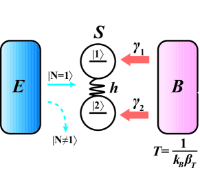
Figure 1: Illustration of a thermal $\mathcal{PT}$ system that comes from the controlled open quantum system S coupling to two separated environments B and E. S denotes a tight-binding model of two lattice sites, $1$ and $2$, with single fermionic particle; B denotes a thermal environment with temperature $T=\frac{1}{k_{B}\beta_{T}}$; and E denotes an environment under postselection with fixed particle number of S to be $1$.

To design a thermal $\mathcal{PT}$ system we couple a thermal bath to a $\mathcal{PT}$ system. To reach this goal, we consider a controlled open quantum system S coupling to two separated environments B and E. (Fig.1) B could thermalize S to its temperature $T=\frac{1}{k_{B}\beta_{T}}$ (we call it thermal environment), and E could lead to a relevant NH term for S under postselection with the fixed particle number of S equal to $1$ (we call it NH environment). The Hamiltonian of the total system is given by

$$\hat{H} =\hat{H}_{\mathrm{S}}\otimes\hat{I}_{\mathrm{E}}\otimes\hat{I}_{\mathrm{B}}+\hat{I}_{\mathrm{S}}\otimes\hat{H}_{\mathrm{E}}\otimes\hat{I}_{\mathrm{B}}$$

$$+\hat{I}_{\mathrm{S}}\otimes\hat{I}_{\mathrm{E}}\otimes\hat{H}_{\mathrm{B}}+\hat{H}_{\mathrm{ES}}\otimes\hat{I}_{\mathrm{B}}+\hat{I}_{\mathrm{E}}\otimes\hat{H}_{\mathrm{BS}},$$ (1)

where $\hat{H}_{\mathrm{S}}=h(c_{1}^{{\dagger}}c_{2}+c_{2}^{{\dagger}}c_{1})$, $\hat{H}_{\mathrm{E}}$, and $\hat{H}_{\mathrm{B}}$ are the Hamiltonians of S, E, and B, respectively. $\hat{H}_{\mathrm{ES}}=\lambda[a^{\dagger}(c_{1}-ic_{2})+h.c.]$ stands for the coupling between S and E that leads to a Lindblad operator $\hat{L}_{\mathrm{ES}}=\sqrt{2\gamma}(c_{1}+ic_{2})\otimes\hat{I}_{\mathrm{B}}$. $\hat{H}_{\mathrm{BS}}=\gamma_{1}c_{1}^{{\dagger}}c_{1}\otimes\hat{B}_{1}+\gamma_{2}c_{2}^{{\dagger}}c_{2}\otimes\hat{B}_{2}$ describes the coupling between S and B, where $\hat{B}_{1}$ and $\hat{B}_{2}$ are the operators of the system B. Here, we assume that $\gamma_{1},\gamma_{2}<<\gamma,h.$ In particular, there is no direct coupling between the two environments B and E. In the following parts, $h$ is set be the unit.

For the open quantum system S under the Markovian approximation, its non-unitary dynamics is in general expressed by the quantum master equation in the Gorini-Kossakowski-Sudarshan-Lindblad (GKSL) form Lindblad76 ; GKS76 ; BreuerPetruccione , $\frac{d\rho^{\mathrm{S}}(t)}{dt}\equiv\mathcal{L}\rho^{\mathrm{S}}(t)$, where $\mathcal{L}$ is a Liouville super-operator acting on the (reduced) density matrix $\rho^{\mathrm{S}}$ of the subsystem S.

In Hermitian systems at finite-T, the quantum statistical mechanics is based on the thermal equilibrium state. To reach it, one can prepare a unique final state under time-evolution (from an arbitrary initial state). Using a similar logic, we introduce a “non-Hermitian thermal state” (NHTS) which is the unique final state under time-evolution in a NH system at finite-T (from an arbitrary initial state). We then give its rigorous mathematical definition as follows:

In thermal $\mathcal{PT}$ systems, if the spectrum of Liouville super-operator $\mathcal{L}$ is $\lambda_{i},$ i.e., $\mathcal{L}\rho_{i}^{\mathrm{S}}=\lambda_{i}\rho_{i}^{\mathrm{S}},$ then a non-Hermitian thermal state described by $\rho_{NHTS}^{\mathrm{S}}$ is the eigenstate of $\mathcal{L}$ corresponding to the eigenvalue with the maximum real part $\lambda_{NHTS}=\max(\operatorname{Re}\lambda_{i})$.

From the above definition, we need to find the possible NHTS by solving the GKSL equation in order to explore the properties of this thermal $\mathcal{PT}$ system.

First, we trace out E from the total system and consider its effect on the combined subsystem S+B. The GKSL equation of the reduced density matrix $\rho^{\mathrm{S+B}}$ for the combined subsystem S+B becomes

$$\frac{d\rho^{\mathrm{S+B}}}{dt} =-i[\hat{H}_{\mathrm{S+B}},\rho^{\mathrm{S+B}}]$$

$$-\frac{1}{2}\{\hat{L}_{\mathrm{ES}}^{{\dagger}}\hat{L}_{\mathrm{ES}},\rho^{\mathrm{S+B}}\}+\hat{L}_{\mathrm{ES}}\rho^{\mathrm{S+B}}\hat{L}_{\mathrm{ES}}^{{\dagger}}.$$ (2)

We make the postselection measurement for the number of particles of the subsystem S $\left(c_{1}^{{\dagger}}c_{1}+c_{2}^{{\dagger}}c_{2}\right)\otimes\hat{I}_{\mathrm{B}}$ so that it is always $1$ Aharonov1988 . After these postselection measurements, the quantum jumping term from $\hat{L}_{\mathrm{ES}}\rho^{\mathrm{S+B}}\hat{L}_{\mathrm{ES}}^{{\dagger}}$ will be projected out Ueda2020 . Then $\rho^{\mathrm{S+B}}$ satisfies

$$\frac{d\rho^{\mathrm{S+B}}}{dt}=-i(\hat{H}_{\mathrm{S+B},\mathrm{eff}}\rho^{\mathrm{S+B}}-\rho^{\mathrm{S+B}}\hat{H}_{\mathrm{S+B},\mathrm{eff}}^{\dagger}),$$ (3)

where $\hat{H}_{\mathrm{S+B},\mathrm{eff}}=\hat{H}_{\mathrm{NH}}\otimes\hat{I}_{\mathrm{B}}+\hat{I}_{\mathrm{S}}\otimes\hat{H}_{\mathrm{B}}+\hat{H}_{\mathrm{BS}}$ is the effective Hamiltonian of the combined subsystem S+B after postselection measurements, and $\hat{H}_{\mathrm{NH}}=(h+\gamma)c_{1}^{{\dagger}}c_{2}+(h-\gamma)c_{2}^{{\dagger}}c_{1}-i\gamma$ can effectively describe the subsystem S. Here, the term $-i\gamma$ in $\hat{H}_{\mathrm{NH}}$ can be ignored due to postselections Yuto2018 ; Todda2002 .

In short, $\hat{H}_{\mathrm{NH}}$ can be effectively expressed as $\hat{H}_{\mathrm{NH}}=h\sigma_{x}+i\gamma\sigma_{y}$ on the pseudo-spin space $(\begin{array}[c]{c}\left|\uparrow\right\rangle\\ \left|\downarrow\right\rangle\end{array})$, where $\left|\uparrow\right\rangle$ and $\left|\downarrow\right\rangle$ denote the quantum states of the single fermion on site $1$ and site $2$, respectively. For $\hat{H}_{\mathrm{NH}}$, at $h=\gamma$, a usual $\mathcal{PT}$-symmetry spontaneous breaking ($\mathcal{PT}$-SSB) occurs: for the case $h>\gamma,$ the energy levels $\left|+\right\rangle$ and $\left|-\right\rangle$ are $E_{\pm}=\pm\sqrt{h^{2}-\gamma^{2}}$; for the case $h<\gamma,$ the energy levels $\left|+\right\rangle$ and $\left|-\right\rangle$ are $E_{\pm}=\pm i\sqrt{\gamma^{2}-h^{2}}$; and for the case $h=\gamma,$ the system is at the EP with state coalescing and energy degeneracy, i.e., $E_{\pm}=0$.

Next, we trace out B from the combined subsystem S+B and consider it on the NH subsystem S. This issue of NH open quantum systems has never been studied before. We assume that the NH subsystem S has little influence on the environment B and the relaxation time of the environment B is much smaller than S. Besides these conditions, the temperature of a possible NHTS is also assumed to be the same as that of the thermal environment B.

On one hand, we study the possible NHTS $\rho_{NHTS}^{\mathrm{S}}$ in the phase with $\mathcal{PT}$-symmetry ($h>\gamma$). Now, the two energy levels of NH Hamiltonian are purely real, $\pm\sqrt{\gamma^{2}-h^{2}}$. As a result, the NHTS must be a steady state with the eigenvalue $0$ corresponding to the Liouville super-operator $\mathcal{L}.$ After solving the GKSL equation, $\rho_{NHTS}^{\mathrm{S}}$ is obtained as $\frac{h-\gamma}{2h}\begin{pmatrix}\frac{h+\gamma}{h-\gamma}&\sqrt{\frac{h+\gamma}{h-\gamma}}\frac{1-e^{\omega_{0}\beta_{T}}}{1+e^{\omega_{0}\beta_{T}}}\\ \sqrt{\frac{h+\gamma}{h-\gamma}}\frac{1-e^{\omega_{0}\beta_{T}}}{1+e^{\omega_{0}\beta_{T}}}&1\end{pmatrix}.$ More detailed calculations are provided in the Supplementary Materials.

On the other hand, we study the possible NHTS $\rho_{NHTS}^{\mathrm{S}}$ in the phase with $\mathcal{PT}$-symmetry breaking ($h<\gamma$). Under the conditions $\gamma_{1},\gamma_{2}<<\gamma,h$, the dissipation term in the Liouville super-operator only has little effect, i.e. $\mathcal{L}\rho^{\mathrm{S}}\approx-i(\hat{H}_{\mathrm{NH}}\rho^{\mathrm{S}}-\rho^{\mathrm{S}}\hat{H}_{\mathrm{NH}}^{\dagger}).$ Now, the eigenvalues of the super-operator $\mathcal{L}$ are obtained as $-2\sqrt{\gamma^{2}-h^{2}},$ $0,$ $0,$ $2\sqrt{\gamma^{2}-h^{2}}$. The eigenstate with the maximum real part $2\sqrt{\gamma^{2}-h^{2}}$ corresponds to a NHTS $\rho_{NHTS}^{\mathrm{S}}=|\Psi_{+}^{\mathrm{R}}\rangle\langle\Psi_{+}^{\mathrm{R}}|.$ This can be understood as the fact that the state $|\Psi_{-}^{\mathrm{R}}\rangle$ decays much more faster than the state $|\Psi_{+}^{\mathrm{R}}\rangle$. Eventually, there is only one eigenstate $|\Psi_{+}^{\mathrm{R}}\rangle$ with the largest imaginary part of the eigenvalue $+i\sqrt{\gamma^{2}-h^{2}}$ left in the system.

Finally, according to the above results from the GKSL equation, we investigate the properties of NHTSs in the thermal $\mathcal{PT}$ system. These results of the expected values of $\sigma_{i}$ ($i=x,y,z$), i.e. $n_{i}=\left\langle\sigma_{i}\right\rangle$, are represented by points on the Bloch sphere in Fig.2(a) and Fig.2(b). Fig.2(a) indicates the existence of a unique NHTS $\rho_{NHTS}^{\mathrm{S}}$: for $\hat{H}_{\mathrm{NH}}$ with fixed $\gamma$ ($\gamma=0.2h$), taking the limit $t\rightarrow\infty$, different initial states will eventually evolve into the same final state $\rho^{\mathrm{S}}(t\rightarrow\infty)$. That means $\rho^{\mathrm{S}}(t\rightarrow\infty)$ is just the NHTS $\rho_{NHTS}^{\mathrm{S}}$; Fig.2(b) indicates the abnormality of the NHTS $\rho_{NHTS}^{\mathrm{S}}$: for $\hat{H}_{\mathrm{NH}}$ with different values for $\gamma$ ($\gamma=0.3h,$ $\gamma=0.9h$, $\gamma=1.5h$), from the same initial state, for example, a fully thermalized state described by $\rho^{\mathrm{S}}(t=0)=\frac{1}{2}I_{2\times 2}$, the system will eventually evolve into different NHTSs $\rho_{NHTS}^{\mathrm{S}}(\gamma)$.

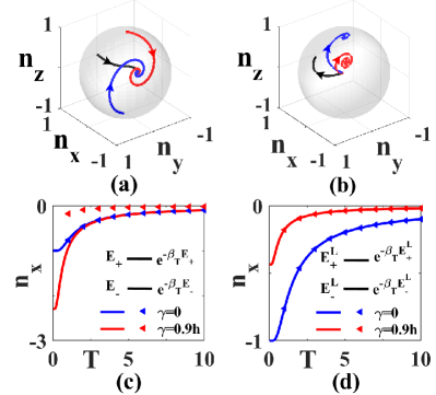
Figure 2: (a) Time-evolution of non-Hermitian (NH) systems for fixed $\gamma$ ($\gamma=0.2h$) from the different initial states at temperature $k_{B}T=h$, where $\gamma_{0}=0.05h$; (b) Time-evolution of NH systems for different $\gamma$ ($\gamma=0.3h,$ $\gamma=0.9h$, $\gamma=1.5h$) from the same fully thermalized initial state, where $\gamma_{0}=0.05h$ and $k_{B}T=10h$. The arrows denote the direction of time-evolution; (c) The comparison between the results from usual Boltzmann distribution (solid lines) and those obtained by directly solving the Gorini-Kossakowski-Sudarshan-Lindblad (GKSL) equation (the small triangles); (d) The comparison between the results from the Liouvillian-Boltzmann distribution (solid lines) and those derived by directly solving the GKSL equation (the small triangles).

Let us check the validity of the BZ law in this thermal $\mathcal{PT}$ system.

For the Hermitian case ($\gamma=0$), different thermal equilibrium states obey the BZ law, i.e., $P_{+}^{T}=e^{-\beta_{T}E_{+}}$ and $P_{-}^{T}=e^{-\beta_{T}E_{-}}$, where $E_{\pm}=\pm h$ are energy levels. In Fig.2(c), the blue line and blue triangles represent these expected values of $\sigma_{x}$ ($n_{x}$) from the BZ law and those derived by directly solving the GKSL equation, respectively. The consistence between the results from the BZ law and those from the GKSL equation verifies the correctness of both approaches.

Then we study the NH case. For NHTSs with $\gamma=0.9h$, we can also derive $n_{x}$ by using the BZ law, i.e. $n_{x}=\frac{1}{e^{-\beta_{T}E_{-}}+e^{-\beta_{T}E_{+}}}\mathrm{Tr}(\sigma_{x}\cdot e^{-\beta_{T}\hat{H}_{\mathrm{NH}}}).$ In Fig.2(c), the red line and red triangles represent $n_{x}$ from the BZ law and those obtained by directly solving the GKSL equation, respectively. One can see that the results derived by means of the two mentioned approaches are noticeably contradictory in this case, which means that the BZ law does not hold in this situation. Consequently, one can safely conclude that the usual BZ law for thermal equilibrium states in Hermitian systems does not work anymore in NH systems! The immediate questions would be how to understand this violation of the BZ law in NHTSs, and whether there exists a new law that explains these abnormal results for a thermal $\mathcal{PT}$ system.

Before developing a systematic theory, we provide a physical explanation. In fact, NHTSs come from NH systems rather than from free ones. To realize a NH system, we controlled the open thermal $\mathcal{PT}$ system by performing a postselection and projecting out the quantum jumping term. The postselection measurement would result in a continuous information backflow from the NH environment E to the subsystem S Ueda17 . These control actions break down the equal probability of different microscopic states and lead to a new distribution law.

In order to better describe this new distribution law, we develop a quantum Liouvillian statistics theory to systematically and analytically characterize the thermal $\mathcal{PT}$ systems. In particular, it is a new type of distribution, that we call Liouvillian-Boltzmann distribution (LBZ) that governs the distribution of NHTSs at finite-T.

We focus on the case with real energy levels ($h>\gamma$). By doing a similarity transformation (ST) $\mathcal{\hat{S}}=e^{\beta_{\mathrm{NH}}\hat{H}^{\prime}},$ $\hat{H}_{\mathrm{NH}}$ can be transformed into a Hermitian Hamiltonian $\hat{H}_{0}=\sqrt{h^{2}-\gamma^{2}}\sigma_{x}$, i.e., $\hat{H}_{\mathrm{NH}}=\mathcal{\hat{S}}\hat{H}_{0}\mathcal{\hat{S}}^{-1}.$ Here, the real number $\beta_{\mathrm{NH}}=\frac{1}{2}\ln\frac{h+\gamma}{h-\gamma}$ characterizes the strength of the NH terms and the Hermitian operator $\hat{H}^{\prime}=\frac{1}{2}\sigma_{z}$ determines the form of the NH terms. Under the NH TS $\mathcal{\hat{S}}$, the energy levels $E_{\pm}$ of $\hat{H}_{\mathrm{NH}}$ are same to those of the Hermitian model $\hat{H}_{0}.$ The corresponding eigenstates of $\hat{H}_{\mathrm{NH}}$ become $|\Psi_{n}^{\mathrm{R}}\rangle=\mathcal{\hat{S}}|\Psi_{0,n}\rangle$, where $n=\pm$ and $|{\Psi}_{0,n}\rangle$ denotes the normalized eigenstates of $\hat{H}_{0}$. It is obvious that the effect from the NH terms leads to the additional NH TS $\mathcal{\hat{S}}$ that breaks down the equal probability of different microscopic states.

Based on these physical quantities, we define the analytical formula of the density matrix $\rho_{NHTS}^{\mathrm{S}}$.

The density matrix for the thermal state of a NH system at temperature $T=\frac{1}{k_{B}\beta_{T}}$ described by $\hat{H}_{\mathrm{NH}}=\mathcal{\hat{S}}\hat{H}_{0}\mathcal{\hat{S}}^{-1}$ ($\mathcal{\hat{S}}=e^{\beta_{\mathrm{NH}}\hat{H}^{\prime}}$) is given as

$$\rho_{NHTS}^{\mathrm{S}}=\sum_{n=\pm}|\Psi_{n}^{\mathrm{R}}\rangle e^{-\beta_{T}E_{n}}\langle\Psi_{n}^{\mathrm{R}}|=\mathcal{\hat{S}}\rho_{0}\mathcal{\hat{S}}^{\dagger},$$ (4)

where $\rho_{0}$ is the density matrix for Hermitian model $\hat{H}_{0}$. In com , we provide the reason to write down the above equation (4).

To simplify the Liouvillian physics for NHTSs, we introduce an effective Hamiltonian $\hat{H}_{\mathrm{L}}$ as $e^{-\beta_{T}\hat{H}_{\mathrm{L}}}=\mathcal{\hat{S}}(e^{-\beta_{T}\hat{H}_{0}})\mathcal{\hat{S}}^{\dagger}$ or

$$\hat{H}_{\mathrm{L}}=-\frac{1}{\beta_{T}}\ln[\mathcal{\hat{S}}(e^{-\beta_{T}\hat{H}_{0}})\mathcal{\hat{S}}^{\dagger}].$$ (5)

In this paper, we call the temperature-dependent Hamiltonian $\hat{H}_{\mathrm{L}}$ to be Liouvillian Hamiltonian (LH). Its corresponding eigenvalues $E_{n}^{\mathrm{L}}$ and eigenstates are called Liouvillian energy levels and Liouvillian states, respectively. According to $\hat{H}_{\mathrm{L}}=\hat{H}_{\mathrm{L}}^{\dagger}$, $E_{n}^{\mathrm{L}}$ must be real.

For NHTSs in this NH system, although the energy levels do not change under STs, the weights of NHTSs are deformed. Consequently, the usual BZ law $P_{n}^{T}=\frac{1}{Z_{0}}e^{-\beta_{T}E_{n}}$ is replaced by the Liouvillian-Boltzmann distribution (LBZ) law gar ; ma , i.e.,

$$P_{n}^{T}=\frac{1}{Z_{0}}e^{-\beta_{T}E_{n}}\rightarrow P_{n}^{T}=\frac{1}{Z_{NHTS}^{\mathrm{S}}}e^{-\beta_{T}E_{n}^{\mathrm{L}}},$$ (6)

where $E_{n}^{\mathrm{L}}$ is a Liouvillian energy level rather than the energy level $E_{n}$ and $Z_{NHTS}^{\mathrm{S}}=Tr(\rho_{NHTS}^{\mathrm{S}})$ are the partition functions for the NHTS. To distinguish the phenomenon of weights in the thermal $\mathcal{PT}$ system from those in Hermitian thermal systems, we call the corresponding weight $P_{n}^{T}$ the Liouvillian weight.

In particular, when the temperature is high, $\beta_{T}\rightarrow 0$, the density matrix $\rho_{NHTS}^{\mathrm{S}}=e^{-\beta_{T}\hat{H}_{\mathrm{L}}}$ for a NH system with real spectra is reduced to $\rho_{NHTS}^{\mathrm{S}}\sim\mathcal{\hat{S}\hat{S}}^{\dagger}=e^{2\beta_{\mathrm{NH}}\hat{H}^{\prime}}$, and the Liouvillian weight turns into $P_{n}^{T}=\frac{1}{Z_{NHTS}^{\mathrm{S}}}e^{-\beta_{\mathrm{NH}}(-2E_{n}^{\prime})}$, where $E_{n}^{\prime}$ is the “energy levels” of $\hat{H}^{\prime}$.

By employing the quantum Liouvillian statistical theory, we study thermodynamic properties for the NHTSs $\rho_{NHTS}^{\mathrm{S}}$ of the thermal $\mathcal{PT}$ system.

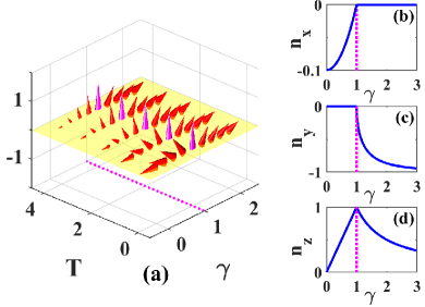
Figure 3: (a) Expected values of the spin operator $n_{i}=\left\langle\sigma_{i}\right\rangle$ from Liouvillian-Boltzmann distribution for the non-Hermitian thermal states $\rho_{NHTS}^{\mathrm{S}}$ of the thermal $\mathcal{PT}$ system. (b), (c), and (d) depict $n_{x}$, $n_{y}$, $n_{z}$ at temperature $k_{B}T=10h$, respectively.

These physical properties of the original NH system $\hat{H}_{\mathrm{NH}}$ at finite-T correspond to those of a Hermitian system of LH, $\hat{H}_{\mathrm{L}}$. According to $e^{-\beta_{T}\hat{H}_{\mathrm{L}}}=\mathcal{\hat{S}}(e^{-\beta_{T}\hat{H}_{0}})\mathcal{\hat{S}}^{\dagger},$ we obtain the analytical result as $e^{-\beta_{T}\hat{H}_{\mathrm{L}}}=\sigma_{x}A+\sigma_{z}B+\mathrm{I}C$, where $\mathrm{I}=(\begin{array}[c]{cc}1&0\\ 0&1\end{array}),$ $A=-\sinh(\beta_{T}\sqrt{h^{2}-\gamma^{2}}),$ $B=\sinh(\beta_{\mathrm{NH}})\cdot\cosh(\beta_{T}\sqrt{h^{2}-\gamma^{2}})$ and $C=\cosh(\beta_{\mathrm{NH}})\cdot\cosh(\beta_{T}\sqrt{h^{2}-\gamma^{2}})$. As a result, the LH is derived as

$$\hat{H}_{\mathrm{L}}=-\frac{1}{\beta_{T}}\frac{\cosh^{-1}C}{\left|\vec{r}_{\mathrm{eff}}\right|}(\vec{\sigma}\cdot\vec{r}_{\mathrm{eff}}),$$

where $\vec{\sigma}=(\sigma_{x},\sigma_{y},\sigma_{z})$, $\vec{r}_{\mathrm{eff}}=(A,0,B)$ and $\left|\vec{r}_{\mathrm{eff}}\right|=\sqrt{A^{2}+B^{2}}$. Hence, the Liouvillian energy levels (the eigenvalues of $\hat{H}_{\mathrm{L}}$) are

$$E_{\pm}^{\mathrm{L}}=\pm\frac{1}{\beta_{T}}\cosh^{-1}\left(\cosh\beta_{\mathrm{NH}}\cdot\cosh(\beta_{T}/2)\right),$$

that are quite different from the energy levels (the eigenvalues for $\hat{H}_{\mathrm{NH}}$) $E_{\pm}=\pm\sqrt{h^{2}-\gamma^{2}}$. According to LBZ law, we have

$$P_{n}^{T}=\frac{1}{Z_{NHTS}^{\mathrm{S}}}\exp[\frac{\cosh^{-1}C}{\left|\vec{r}_{\mathrm{eff}}\right|}(\vec{\sigma}\cdot\vec{r}_{\mathrm{eff}})].$$

The expected values of $\sigma_{i}$ ($i=x,y,z$) are defined as $n_{i}=\left\langle\sigma_{i}\right\rangle=\frac{1}{Z_{NHTS}^{\mathrm{S}}}\mathrm{Tr}(\sigma_{i}\cdot e^{-\beta_{T}\hat{H}_{\mathrm{L}}}).$

After straightforward calculations, we have $\vec{n}=(n_{x},n_{y},n_{z})=(\frac{A}{C},0,\frac{B}{C})$ in the region of $h>\gamma$. We then check the validity of the LBZ law by comparing its results ($n_{x}=\frac{A}{C}$) with those from solving the GKSL equation. As shown in Fig.2(d), they have the exact consistence of those derived by directly solving the GKSL equation (small triangles). Fig.3(a) shows the results of $\vec{n}$. From it, one can see that when $\beta_{\mathrm{NH}}$ increases from zero to infinite, the spin direction changes from the $x$-direction to the $z$-direction. Fig.3(b)-(d) show the behavior of $n_{i}=\left\langle\sigma_{i}\right\rangle$ at $k_{B}T=10h$, respectively. Approaching to EP $h\rightarrow\gamma$ (or $\beta_{\mathrm{NH}}\rightarrow\infty$), we have $\hat{H}_{\mathrm{L}}\rightarrow\frac{\beta_{\mathrm{NH}}}{\beta_{T}}\sigma_{z}$ at finite-T. The external field $\left|\frac{\beta_{\mathrm{NH}}}{\beta_{T}}\right|$ in LH $\hat{H}_{\mathrm{L}}$ becomes infinite. As a result, $\vec{n}$ is fixed to be polarized along the $z$-direction with saturated amplitude $1$ (See the magenta arrows in Fig.2(a)) marked by a magenta line). For the region of $h<\gamma$, the NHTS becomes a pure state described by $|\Psi_{+}^{\mathrm{R}}\rangle$ and we have $\vec{n}=(0,-\sqrt{1-(\frac{h}{\gamma})^{2}},\frac{h}{\gamma})$. As shown in Fig.2(a), the red arrows (the expected values of $\sigma_{i}$) swerve from the $z$-direction to the $y$-direction with increasing $\gamma$.

Finally, we discuss the possible thermodynamic phase transition at the EP $\ h=\gamma$.

From the above discussions we concluded that the average spin operator $n_{i}$ is always continuous when crossing over the EP. Furthermore, we calculate the derivatives of spin average values $\frac{\partial\vec{n}}{\partial\gamma}$. Because $h=\gamma$ is a transition from real spectra to complex, the NHTSs of both sides ($h>\gamma$ and $h<\gamma$) are described by different functions. Thus, $\frac{\partial\vec{n}}{\partial\gamma}$ becomes discontinuous at $h=\gamma$. The discontinuity of $\frac{\partial\vec{n}}{\partial\gamma}$ indicates a “continuous” thermodynamic phase transition. In particular, there exists a $\nu=\frac{1}{2}$ critical rule for $\frac{\partial\vec{n}}{\partial\gamma}$: at finite-T $T\neq 0$, $\frac{\partial\vec{n}}{\partial\gamma}=(2\beta_{T},0,h^{-1})$ for $h\rightarrow\gamma+0^{+}$ and $\frac{\partial\vec{n}}{\partial\gamma}=(0,-(2h)^{{}^{-\frac{1}{2}}}(\gamma-h)^{-\nu},-\gamma^{-1})$ for $\gamma\rightarrow h+0^{+}$; at zero temperature $T=0$, $\frac{\partial\vec{n}}{\partial\gamma}=((2h)^{-\frac{1}{2}}(h-\gamma)^{-\nu},0,h^{-1})$ for $h\rightarrow\gamma+0^{+}$ and $\frac{\partial\vec{n}}{\partial\gamma}=(0,-(2h)^{-\frac{1}{2}}(\gamma-h)^{-\nu},-\gamma^{-1})$ for $\gamma\rightarrow h+0^{+}$. To emphasize the strangeness of the $\nu=\frac{1}{2}$ critical rule, we call it zero temperature anomaly for the thermodynamic phase transition at EP. See the detailed calculations in the Supplementary Materials.

In this paper we studied the physics of thermal $\mathcal{PT}$ systems. Our results show that due to the postselection measurements, for the thermal $\mathcal{PT}$ system both the usual BZ law and Equal Probability Principle do not hold anymore. To characterize this abnormal behavior in NH systems at finite-T, a quantum Liouvillian statistics theory was developed, where the usual BZ law $P_{n}^{T}\sim e^{-E_{n}/k_{B}T}$ is replaced by the LBZ law $P_{n}^{T}\sim e^{-E_{n}^{\mathrm{L}}/k_{B}T}$, where $E_{n}^{\mathrm{L}}$ is a Liouvillian energy level rather than an energy level $E_{n}$. Based on the new theory, analytical results of thermodynamic properties for the thermal $\mathcal{PT}$ system were derived. We found that a “continuous” thermodynamic phase transition occurs at the EP, where there exists a zero-temperature anomaly. In the future, we plan to study the thermal states of more complex NH models and to explore the possible exotic phenomena in NH systems at finite-T.

References

(1)C. M. Bender, and S. Boettcher, Phys. Rev. Lett.
80, 5243 (1998).
(2)C. M. Bender, D. C. Brody, and H. F. Jones, Phys. Rev.
Lett. 89, 270401 (2002).
(3)C. M. Bender, Rep. Prog. Phys. 70, 947 (2007).
(4)G. L Giorgi, Phys. Rev. B 82, 052404 (2010).
(5)L. Ge and H. E. Türeci, Phys. Rev. A 88, 053810 (2013).
(6)C. Hang, G. Huang, and V. V. Konotop, Phys. Rev. Lett.
110, 083604 (2013).
(7)C. Korff and R. Weston, J. Phys. A 40, 8845 (2007).
(8)C. Korff and R. Weston, J. Phys. A 41, 295206 (2008).
(9)C. E. Rüter, K. G. Makris, R. El-Ganainy, D. N.
Christodoulides, M. Segev, and D. Kip, Nat. Phys. 6, 192 (2010).
(10)C. Hang, G. Huang, and V. V. Konotop, Phys. Rev. Lett.
110, 083604 (2013).
(11)A. Guo, G. J. Salamo, D. Duchesne and R. Morandotti, M.
Volatier-Ravat and V. Aimez, G. A. Siviloglou and D. N. Christodoulides, Phys.
Rev. Lett. 103, 093902 (2009).
(12)P. Peng W. Cao, C. Shen, W. Qu, J. Wen, L. Jiang and Y. Xiao,
Nat. Phys. 12, 1139 (2016).
(13)Z. Zhang, Y. Zhang, J. Sheng, L. Yang, M.-A. Miri, D. N.
Christodoulides, B. He, Y. Zhang, and M. Xiao, Phys. Rev. Lett. 117,
123601 (2016).
(14)Y. D. Chong, Li Ge, and A. Douglas Stone, Phys. Rev. Lett.
106, 093902 (2011).
(15)A. Regensburger, C. Bersch, M.-A. Miri, G. Onishchukov, D.
N. Christodoulides, and U. Peschel, Nature (London) 488, 167 (2012).
(16)L. Feng, Y.-L. Xu, W. S. Fegadolli, M.-H. Lu, J. E. B.
Oliveira, V. R. Almeida, Y.-F. Chen, and A. Scherer, Nat. Mater. 12,
108 (2013).
(17)M. Wimmer, M.-A. Miri, D. Christodoulides, and U. Peschel,
Sci. Rep. 5, 17760 (2015).
(18)S. Weimann, M. Kremer, Y. Lumer, S. Nolte, K. G. Makris, M.
Segev, M. C. Rechtsman and A. Szameit, Nat. Mater. 16, 433 (2017).
(19)H. Hodaei, A. U. Hassan, S. Wittek, H. Garcia-Gracia, R.
El-Ganainy, D. N. Christodoulides, and M. Khajavikhan, Nature 548,
187 (2017).
(20)S. K. Özdemir, S. Rotter, F.Nori, and L. Yang, Nat. Mater.
18, 783 (2019).
(21)L. Feng, Y. L. Xu, W. S. Fegadolli, M. H. Lu, J. E. B.
Oliveira, V. R. Almeida, Y. F. Chen and A. Scherer, Nat. Mater. 12,
108 (2013).
(22)J. Li, A. K. Harter, J. Liu, L. de Melo, Y. N. Joglekar and L.
Luo , Nat. Commun. 10, 855 (2019).
(23)N. Bender, S. Factor, J. D. Bodyfelt, H. Ramezani, D. N.
Christodoulides, F. M. Ellis, and T. Kottos, Phys. Rev. Lett. 110,
234101 (2013).
(24)J. Schindler, A. Li, M. C. Zheng, F. M. Ellis, and T.
Kottos, Phys. Rev. A 84, 040101(R) (2011).
(25)S. Assawaworrarit, X. Yu, S. Fan, Nature
546, 387 (2017).
(26)Y. Choi, C. Hahn, J. W. Yoon, and S. H. Song, Nat. Commun.
9, 2182 (2018).
(27)S. Bittner, B. Dietz, U. Günther, H. L. Harney, M.
Miski-Oglu, A. Richter, and F. Schäfer, Phys. Rev. Lett. 108,
024101 (2012).
(28)B. Peng, S. K. Özdemir, F. Lei, F. Monifi, M. Gianfreda, G.
L. Long, S. Fan, F. Nori, C. M. Bender, and L. Yang, Nat. Phys. 10,
394 (2014).
(29)C. Poli, M. Bellec, U. Kuhl, F. Mortessagne, and H.
Schomerus, Nat. Commun. 6, 6710 (2015).
(30)Z.-P. Liu, J. Zhang, S. K. Özdemir, B. Peng, H. Jing,
X.-Y. Lü, C.-W. Li, L. Yang, F. Nori, and Y.-X. Liu, Phys. Rev. Lett.
117, 110802 (2016).
(31)L. Feng, Z. J. Wong, R. M. Ma, Y. Wang and X. Zhang, Science,
346 972 (2014).
(32)B. Peng, S. K. Özdemir, F. Lei, F. Monifi, M. Giandreda,
G. L. Long S. Fan, F. Nori, C. M. Bender and L. Yang, Nat. Phys. 10,
394 (2014).
(33)H. Hodaei, M. A. Miri, M. Heinrich, D. N. Christodoulides,
M. Khajavikhan, Science, 346, 975 (2014).
(34)X. Zhu, H. Ramezani, C. Shi, J. Zhu, and X. Zhang, Phys. Rev.
X 4, 031042 (2014).
(35)B.-I. Popa, and S. A. Cummer, Nat. Commun. 5, 3398 (2014).
(36)R. Fleury, D. Sounas, and A. Alù, Nat. Commun.
6, 5905 (2015).
(37)K. Ding, G. Ma, M. Xiao, Z. Q. Zhang, and C. T. Chan, Phys.
Rev. X 6, 021007 (2016).
(38)Y. Wu, W. Liu, J. Geng, X. Song, X. Ye, C. K. Duan, X. Rong,
and J. Du, Science, 364, 878 (2019).
(39)K. Kawabata, Y. Ashida, and M. Ueda, Phys. Rev. Lett.
119, 190401 (2017).
(41)V. Gorini, A. Kossakowski, and E. C. G. Sudarshan, J. Math.
Phys., 17, 821 (1976).
(42)H. P. Breuer and F. Petruccione,
The Theory of Open Quantum Systems (Oxford University Press, Oxford, 2002).
(43)Y. Aharonov, D. Z. Albert, and L. Vaidman, Phys. Rev.
Lett. 60, 1351 (1988); Y. Aharonov and L. Vaidman, Phys. Rev. Lett.
62, 2327 (1989); A. J. Leggett, Phys. Rev. Lett. 62, 2325
(1989); A. Peres, Phys. Rev. Lett. 62, 2326 (1989); Y. Aharonov and
L. Vaidman, Phys. Rev. A 41, 11 (1990).
(44)N. Matsumoto, K. Kawabata, Y. Ashida, S. Furukawa, and M.
Ueda, Phys. Rev. Lett. 125, 260601 (2020).
(45)T. A. Brun, Am. J. Phys. 70, 719 (2002).
(46)Y. Ashida and M. Ueda, Phys. Rev. Lett. 120,
185301 (2018).
(47)Let briefly explain why the density matrix is defined as
To develop a theory to describe quantum
statistical physics of non-Hermitian systems, there are two choices:
one choice is to define density matrix , the other
is . From the results by solving GKSL equation,
we found is real. However, the density matrix
is always complex, i.e.,
; the density matrix
is real, i.e.,
Therefore, we may
guess the density matrix from is
correct. Furthermore, to confirm the conclusion, we do both calculations from
directly solving GKSL equation and those from . The consistence between the results from them verifies
the correctness of the definition of .
(48)B. Gardas, S. Deffner and A. Saxena, Scientific Reports
6, 23408 (2016).
(49)P. N. Meisinger and M. C. Ogilvie, Phil. Trans. R. Soc. A
371, 20120058 (2013).