Improving Multimodal Fusion with Hierarchical Mutual Information Maximization for Multimodal Sentiment Analysis

Abstract

In multimodal sentiment analysis (MSA), the performance of a model highly depends on the quality of synthesized embeddings. These embeddings are generated from the upstream process called multimodal fusion, which aims to extract and combine the input unimodal raw data to produce a richer multimodal representation. Previous work either back-propagates the task loss or manipulates the geometric property of feature spaces to produce favorable fusion results, which neglects the preservation of critical task-related information that flows from input to the fusion results. In this work, we propose a framework named MultiModal InfoMax (MMIM), which hierarchically maximizes the Mutual Information (MI) in unimodal input pairs (inter-modality) and between multimodal fusion result and unimodal input in order to maintain task-related information through multimodal fusion. The framework is jointly trained with the main task (MSA) to improve the performance of the downstream MSA task. To address the intractable issue of MI bounds, we further formulate a set of computationally simple parametric and non-parametric methods to approximate their truth value. Experimental results on the two widely used datasets demonstrate the efficacy of our approach. The implementation of this work is publicly available at https://github.com/declare-lab/Multimodal-Infomax.

1 Introduction

With the unprecedented advances in social media in recent years and the availability of smartphones with high-quality cameras, we witness an explosive boost of multimodal data, such as movies, short-form videos, etc. In real life, multimodal data usually consists of three channels: visual (image), acoustic (voice), and transcribed text. Many of them often express sort of sentiment, which is a long-term disposition evoked when a person encounters a specific topic, person or entity (Deonna and Teroni, 2012; Poria et al., 2020). Mining and understanding these emotional elements from multimodal data, namely multimodal sentiment analysis (MSA), has become a hot research topic because of numerous appealing applications, such as obtaining overall product feedback from customers or gauging polling intentions from potential voters (Melville et al., 2009). Generally, different modalities in the same data segment are often complementary to each other, providing extra cues for semantic and emotional disambiguation (Ngiam et al., 2011). The crucial part for MSA is multimodal fusion, in which a model aims to extract and integrate information from all input modalities to understand the sentiment behind the seen data. Existing methods to learn unified representations are grouped in two categories: through loss back-propagation or geometric manipulation in the feature spaces. The former only tunes the parameters based on back-propagated gradients from the task loss (Zadeh et al., 2017; Tsai et al., 2019a; Ghosal et al., 2019), reconstruction loss (Mai et al., 2020), or auxiliary task loss (Chen et al., 2017; Yu et al., 2021). The latter additionally rectifies the spatial orientation of unimodal or multimodal representations by matrix decomposition (Liu et al., 2018) or Euclidean measure optimization (Sun et al., 2020; Hazarika et al., 2020). Although having gained excellent results in MSA tasks, these methods are limited to the lack of control in the information flow that starts from raw inputs till the fusion embeddings, which may risk losing practical information and introducing unexpected noise carried by each modality Tsai et al. (2020). To alleviate this issue, different from previous work, we leverage the functionality of mutual information (MI), a concept from the subject of information theory. MI measures the dependencies between paired multi-dimensional variables. Maximizing MI has been demonstrated efficacious in removing redundant information irrelevant to the downstream task and capturing invariant trends or messages across time or different domains (Poole et al., 2019), and has been shown remarkable success in the field of representation learning Hjelm et al. (2018); Veličković et al. (2018). Based on these experience, we propose MultiModal InfoMax (MMIM), a framework that hierarchically maximizes the mutual information in multimodal fusion. Specifically, we enhance two types of mutual information in representation pairs: between unimodal representations and between fusion results and their low-level unimodal representations. Due to the intractability of mutual information (Belghazi et al., 2018), researchers always boost MI lower bound instead for this purpose. However, we find it is still difficult to figure out some terms in the expressions of these lower bounds in our formulation. Hence for convenient and accurate estimation of these terms, we propose a hybrid approach composed of parametric and non-parametric parts based on data and model characteristics. The parametric part refers to neural network-based methods, and in the non-parametric part we exploit a Gaussian Mixture Model (GMM) with learning-free parameter estimation. Our contributions can be summarized as follows:

1. We propose a hierarchical MI maximization framework for multimodal sentiment analysis. MI maximization occurs at the input level and fusion level to reduce the loss of valuable task-related information. To our best knowledge, this is the first attempt to bridge MI and MSA.

2. We formulate the computation details in our framework to solve the intractability problem. The formulation includes parametric learning and non-parametric GMM with stable and smooth parameter estimation.

3. We conduct comprehensive experiments on two publicly available datasets and gain superior or comparable results to the state-of-the-art models.

2 Related Work

In this section, we briefly overview some related work in multimodal sentiment analysis and mutual information estimation and application.

2.1 Multimodal Sentiment Analysis (MSA)

MSA is an NLP task that collects and tackles data from multiple resources such as acoustic, visual, and textual information to comprehend varied human emotions (Morency et al., 2011). Early fusion models adopted simple network architectures, such as RNN based models (Wöllmer et al., 2013; Chen et al., 2017) that capture temporal dependencies from low-level multimodal inputs, SAL-CNN (Wang et al., 2017) which designed a select-additive learning procedure to improve the generalizability of trained neural networks, etc. Meanwhile, there were many trials to combine geometric measures as accessory learning goals into deep learning frameworks. For instance, Hazarika et al. (2018); Sun et al. (2020) optimized the deep canonical correlation between modality representations for fusion and then passed the fusion result to downstream tasks. More recently, formulations influenced by novel machine learning topics have emerged constantly: Akhtar et al. (2019) presented a deep multi-task learning framework to jointly learn sentiment polarity and emotional intensity in a multimodal background. Pham et al. (2019) proposed a method that cyclically translates between modalities to learn robust joint representations for sentiment analysis. Tsai et al. (2020) proposed a routing procedure that dynamically adjusts weights among modalities to provide interpretability for multimodal fusion. Motivated by advances in the field of domain separation, Hazarika et al. (2020) projected modality features into private and common feature spaces to capture exclusive and shared characteristics across different modalities. Yu et al. (2021) designed a multi-label training scheme that generates extra unimodal labels for each modality and concurrently trained with the main task.

In this work, we build up a hierarchical MI-maximization guided model to improve the fusion outcome as well as the performance in the downstream MSA task, where MI maximization is realized not only between unimodal representations but also between fusion embeddings and unimodal representations.

2.2 Mutual Information in Deep Learning

Mutual information (MI) is a concept from information theory that estimates the relationship between pairs of variables. It is a reparameterization-invariant measure of dependency (Tishby and Zaslavsky, 2015) defined as:

$$I(X;Y)=\mathbb{E}_{p(x,y)}\left[\log\frac{p(x,y)}{p(x)p(y)}\right]$$ (1)

Alemi et al. (2016) first combined MI-related optimization into deep learning models. From then on, numerous works studied and demonstrated the benefit of the MI-maximization principle (Bachman et al., 2019; He et al., 2020; Amjad and Geiger, 2019). However, since direct MI estimation in high-dimensional spaces is nearly impossible, many works attempted to approximate the true value with variational bounds (Belghazi et al., 2018; Cheng et al., 2020; Poole et al., 2019).

In our work, we apply MI lower bounds at both the input level and fusion level and formulate or reformulate estimation methods for these bounds based on data characteristics and mathematical properties of the terms to be estimated.

3 Method

3.1 Problem Definition

In MSA tasks, the input to a model is unimodal raw sequences $X_{m}\in\mathbb{R}^{l_{m}\times d_{m}}$ drawn from the same video fragment, where $l_{m}$ is the sequence length and $d_{m}$ is the representation vector dimension of modality $m$, respectively. Particularly, in this paper we have $m\in\{t,v,a\}$, where $t,v,a$ denote the three types of modalities—text, visual and acoustic that we obtained from the datasets. The goal for the designed model is to extract and integrate task-related information from these input vectors to form a unified representation and then utilize that to make accurate predictions about a truth value $y$ that reflects the sentiment strength.

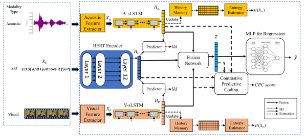
Figure 1: The overall architecture of the MMIM model.

3.2 Overall Architecture

As shown in Figure 1, our model firstly processes raw input into numerical sequential vectors with feature extractor (firmware for visual and acoustic with no parameters to train) and tokenizer (for text). Then we encode them into individual unit-length representations. The model then works in two collaborative parts—fusion and MI maximization, marked by solid and dash lines in Figure 1 respectively. In the fusion part, a fusion network $F$ of stacked linear-activation layers transforms the unimodal representations into the fusion result $Z$, which is then passed through a regression multilayer perceptron (MLP) for final predictions. In the MI part, the MI lower bounds at two levels—input level and fusion level are estimated and boosted. The two parts work concurrently to produce task and MI-related losses for back-propagation, through which the model learns to infuse the task-related information into fusion results as well as improve the accuracy of predictions in the main task.

3.3 Modality Encoding

We firstly encode the multimodal sequential input $X_{m}$ into unit-length representations $h_{m}$. Specifically, we use BERT (Devlin et al., 2019) to encode an input sentence and extract the head embedding from the last layer’s output as $h_{t}$. For visual and acoustic, following previous works (Hazarika et al., 2020; Yu et al., 2021), we employ two modality-specific unidirectional LSTMs (Hochreiter and Schmidhuber, 1997) to capture the temporal features of these modalities:

$$\begin{gathered}h_{t}=\textrm{BERT}\left(X_{t};\theta_{t}^{BERT}\right)\\ h_{m}=\textrm{sLSTM}\left(X_{m};\theta_{m}^{LSTM}\right)\;m\in\{v,a\}\end{gathered}$$ (2)

3.4 Inter-modality MI Maximization

For a modality representation pair $X,Y$ that comes from a single video clip, although they seem to be independent sequences, there is a certain correlation between them Arandjelovic and Zisserman (2017). Formally, suppose we have a collection of videos $V$ and assume that their prior distributions are known. Then the prior distribution of $X$ and $Y$ can be decomposed by the sampling process in $V$ as $P(X)=\int_{V}P(X|V)P(V)$ and $P(Y)=\int_{V}P(Y|V)P(V)$, as well as their joint distribution $P(X,Y)=\int_{V}P(X,Y|V)P(V)$. Unless $P(X,Y|V)=P(X|V)P(Y|V)$, i.e., $X$ and $Y$ are conditionally independent from $V$, the MI is never trivially 0.

Since the analysis above, we hope that through prompting MI between multimodal input we can filter out modality-specific random noise that is irrelevant to our task and keep modality-invariant contents that span all modalities as much as possible. As stated before, we boost a tractable lower bound instead of computing MI directly for this purpose. We exploit an accurate and straightforward MI lower bound introduced in Barber and Agakov (2004). It approximates the truth conditional distribution $p(y|x)$ with a variational counterpart $q(y|x)$:

$$I(X;Y)= \mathbb{E}_{p(x,y)}\left[\log\frac{q(y|x)}{p(y)}\right]+$$ (3)

$$\mathbb{E}_{p(y)}\left[KL(p(y|x)\|q(y|x))\right]$$

$$\geq \mathbb{E}_{p(x,y)}\left[\log q(y|x)\right]+H(Y)$$

$$\triangleq I_{BA}$$

where $H(Y)$ is the differential entropy of $Y$. This lower bound is tight, i.e., there is no gap between the bound and truth value, when $q(y|x)=p(y|x)$. In our implementation, we optimize the bounds for two modality pairs— (text, visual) and (text, acoustic). In each pair, we treat text as $X$ and the other modality as $Y$ in (3). We do so because 1) Since we have to train a predictor $q(y|x)$ to approximate $p(y|x)$, prediction from higher-dimensional vectors $h_{t}\in\mathbb{R}^{d_{t}}$ ($d_{t}$ =768) to lower ones $h_{v}\in\mathbb{R}^{d_{v}}$ and $h_{a}\in\mathbb{R}^{d_{a}}$ ($d_{v},d_{a}$ ¡ 50) converges faster with higher accuracy; 2) many previous works (Tsai et al., 2019a; Hazarika et al., 2020) pointed out that from empirical study the text modality is predominate, which can integrate more task-related features than other modalities in this step. Additionally, we examine the efficacy of the design choice in the ablation study part. Following Cheng et al. (2020), we formulate $q(\bm{y}|\bm{x})$ as a multivariate Gaussian distributions $q_{\theta}(\bm{y}|\bm{x})=\mathcal{N}(\bm{y}|\bm{\mu}_{\theta_{1}}(\bm{x}),\bm{\sigma}^{2}_{\theta_{2}}(\bm{x})\bm{I})$, with two neural networks parameterized by $\theta_{1}$ and $\theta_{2}$ to predict the mean and variance, respectively. The loss function for likelihood maximization is:

$$\mathcal{L}_{lld}=-\frac{1}{N}\sum_{tv,ta}\sum_{i=1}^{N}\log q(y_{i}|x_{i})$$ (4)

where $N$ is the batch size in training, $tv,ta$ means summing the likelihood of two predictors.

For the entropy term $H(Y)$, we solve its computation with the Gaussian Mixture Model (GMM), a commonly utilized approach for unknown distribution approximation that can facilitate distribution-based estimation (Nilsson et al., 2002; Kerroum et al., 2010). GMM builds up multiple Gaussian distributions for different property classes. We choose the sentiment polarity (non-negative/negative), which is a natural property in the datasets, as the classification criterion, which can also balance the trade-off between estimation accuracy (requires more classes) and computational cost (requires fewer classses). We build up two normal distributions $\mathcal{N}_{pos}(\bm{\mu}_{1},\bm{\Sigma}_{1})$ and $\mathcal{N}_{neg}(\bm{\mu}_{2},\bm{\Sigma}_{2})$ for each class, where $\bm{\mu}$ is the mean vector and $\bm{\Sigma}$ is the covariance matrix. The parameters are estimated via the maximum likelihood method on a sufficiently large sampling batch $\mathcal{D}_{s}\subset\mathcal{D}_{train}$:

$$\begin{gathered}\hat{\bm{\mu}}_{c}=\frac{1}{N_{c}}\sum_{i=1}^{N_{c}}h^{i}_{c}\\ \hat{\bm{\Sigma}}_{c}=\frac{1}{N_{c}}\sum_{i=1}^{N_{c}}h^{i}_{c}\odot h^{i}_{c}-\hat{\bm{\mu}}_{c}^{T}\hat{\bm{\mu}}_{c}\end{gathered}$$ (5)

where $c\in\{pos,neg\}$ represents the polarity class that the sample belongs to, $N_{c}$ is the number of samples in class $c$ and $\odot$ is component-wise multiplication. The entropy of a multivariate normal distribution is given by:

$$H=\frac{1}{2}\log\left((2\pi e)^{k}\det(\bm{\Sigma})\right)=\frac{\log(\det(2\pi e\bm{\Sigma}))}{2}$$ (6)

where $k$ is the dimensionality of the vectors in GMM and $\det(\bm{\Sigma})$ is the determinant of $\bm{\Sigma}$. Based on the nearly equal frequencies of the two polarity classes in the dataset, we assume the prior probability that one data point $\bm{x}=(x_{1},...,x_{k})$ belongs to each is equal, i.e., $w_{pos}=p(\bm{x}\in pos)=w_{neg}=p(\bm{x}\in neg)=\frac{1}{2}$. Under the assumption that the two sub-distributions are disjoint, from Huber et al. (2008) the lower and upper bound of a GMM’s entropy are:

$$\sum_{c}w_{c}h_{c}\leq H(Y)\leq\sum_{c}w_{c}(-\log w_{c}+h_{c})$$ (7)

where $h_{c}$ is the entropy of the sub-distribution for class $c$. Taking the lower bound as an approximation, we obtain the entropy term for the MI lower bound:

$$H(Y)=\frac{1}{4}\left[\log((\det(\bm{\Sigma}_{1})\det(\bm{\Sigma}_{2}))\right]$$ (8)

In this formulation, we implicitly assume that the prior probabilities of the two classes are equal. We further notice that $H(Y)$ changes every time during each training epoch but at a very slow pace in several continuous steps due to the small gradients and consequently slight fluctuation in parameters. This fact demands us to update parameters timely to ensure estimation accuracy. Besides, according to statistical theory, we should increase the batch size ($N_{*}$) to reduce estimation error, but the maximum batch size is restricted to the GPU’s capacity. Considering the situation above, we indirectly enlarge $\mathcal{D}_{s}$ by encompassing the data from the nearest history. In implmentation, we store such data in a history data memory. The loss function for MI lower bound maximization in this level is given by:

$$\mathcal{L}_{BA}=-I_{BA}^{t,v}-I_{BA}^{t,a}$$ (9)

3.5 MI Maximization in the Fusion Level

To enforce the intermediate fusion results to capture modality-invariant cues among modalities, we repeat MI maximization between fusion results and input modalities. The optimization target is the fusion network $F$ that produces fusion results $Z=F(X_{t},X_{v},X_{a})$. Since we already have a generation path from $X_{m}$ to $Z$, we expect an opposite path, i.e. to constructs $X_{m},m\in\{t,v,a\}$ from $Z$. Inspired by but different from Oord et al. (2018), we use a score function that acts on the normalized prediction and truth vectors to gauge their correlation:

$$\begin{gathered}\overline{G_{\phi}(Z)}=\frac{G_{\phi}(Z)}{\|G_{\phi}(Z)\|_{2}},\quad\overline{h_{m}}=\frac{h_{m}}{\|h_{m}\|}_{2}\\ s(h_{m},Z)=\exp{\left(\overline{h_{m}}\left(\overline{G_{\phi}(Z)}\right)^{T}\right)}\end{gathered}$$ (10)

where $G_{\phi}$ is a neural network with parameters $\phi$ that generates a prediction of $h_{m}$ from $Z$, $\|\cdot\|_{2}$ is the Euclidean norm, by dividing which we obtain unit-length vectors. Because we find the model intends to stretch both vectors to maximize the score in (10) without this normalization. Then same as what Oord et al. (2018) did, we incorporate this score function into the Noise-Contrastive Estimation framework (Gutmann and Hyvärinen, 2010) by treating all other representations of that modality in the same batch $\tilde{\mathbf{H}}_{m}^{i}=\mathbf{H}_{m}\setminus\{h_{m}^{i}\}$ as negative samples:

$$\mathcal{L}_{\mathbf{N}}(Z,\mathbf{H}_{m})=-\mathbb{E}_{\mathbf{H}}\left[\log\frac{s(Z,h_{m}^{i})}{\sum_{h_{m}^{j}\in\mathbf{H}_{m}}s(Z,h_{m}^{j})}\right]$$ (11)

Here is a short explanation of the rationality of such formulation. Contrastive Predictive Coding (CPC) scores the MI between context and future elements “across the time horizon” to keep the portion of “slow features” that span many time steps (Oord et al., 2018). Similarly, in our model, we ask the fusion result $Z$ to reversely predict representations “across modalities” so that more modality-invariant information can be passed to $Z$. Besides, by aligning the prediction to each modality we enable the model to decide how much information it should receive from each modality. This insight will be further discussed with experimental evidence in Section 5.2. The loss function for this level is given by:

$$\mathcal{L}_{CPC}=\mathcal{L}_{\mathbf{N}}^{z,v}+\mathcal{L}_{\mathbf{N}}^{z,a}+\mathcal{L}_{\mathbf{N}}^{z,t}$$ (12)

Input: Dataset $\mathcal{D}=\{(X_{t},X_{v},X_{a}),Y\}$, $\alpha$, $\beta$, learning rate $\eta_{lld},\eta_{main}$, embedding history memory $M$

Output: Prediction $\hat{y}$

for each training epoch do

       Stage 1: Conditional Likelihood Maximization

       for minibatch $\mathcal{B}=\{(X_{t}^{i},X_{v}^{i},X_{a}^{i})\}_{i=1}^{N}$ sampled from $\mathcal{D}_{sub}\subseteq\mathcal{D}$ do

             Encode $X_{m}^{i}$ to $h_{m}^{i}$ as (2)

             Compute $\mathcal{L}_{lld}$ as (4)

             Update parameters of predictor $q$: $\theta_{q}\leftarrow\theta_{q}-\eta_{lld}\nabla_{\theta}\mathcal{L}_{lld}$

       end for

      Stage 2: MI-maximization Joint Training:

       for minibatch $\mathcal{B}=\{(X_{t}^{i},X_{v}^{i},X_{a}^{i})\}_{i=1}^{N}$ sampled from $\mathcal{D}$ do

             Encode $X_{m}^{i}$ to $h_{m}^{i}$ as (2)

             Estimate the mean vectors and co-variance matrices in GMM model with $M$ as (5)

             Update history $M$: $M\leftarrow M\setminus\{Oldest\;Hidden\;Batch\}$ $M\leftarrow M\cup\{h_{m}^{i}\}_{i=1}^{|B|},m\in\{v,a\}$

             Compute $\mathcal{L}_{BA}$ as (3), (8), (9)

             Produce fusion results $Z_{i}=F(X_{t}^{i},X_{v}^{i},X_{a}^{i})$ and predictions $\hat{y}$

             Compute $\mathcal{L}_{N}$, $\mathcal{L}_{CPC}$ as (10), (11), (12)

             Compute $\mathcal{L}_{main}$ as (14)

             Update all parameters in the model except $q$: $\theta_{k}\leftarrow\theta_{k}-\eta_{k}\nabla_{\theta}\mathcal{L}_{main}$

       end for

      

end for

Algorithm 1 MultiModal Mutual Information Maximization (MM-MIM)

3.6 Training

The training process consists of two stages in each iteration: In the first stage, we approximate $p(y|x)$ with $q(y|x)$ by minimizing the negative log-likelihood for inter-modality predictors with the loss in (4). In the second stage, hierarchical MI lower bounds in previous subsections are added to the main loss as auxiliary losses. After obtaining the final prediction $\hat{y}$, along with the truth value $y$, we have the task loss:

$$\mathcal{L}_{task}=\textrm{MAE}(\hat{y},y)$$ (13)

where MAE stands for mean absolute error loss, which is a common practice in regression tasks. Finally, we calculate the weighted sum of all these losses to obtain the main loss for this stage:

$$\mathcal{L}_{main}=\mathcal{L}_{task}+\alpha\mathcal{L}_{CPC}+\beta\mathcal{L}_{BA}$$ (14)

where $\alpha,\beta$ are hyper-parameters that control the impact of MI maximization. We summarize the training algorithm in Algorithm 1.

4 Experiments

In this section, we present some experimental details, including datasets, baselines, feature extraction tool kits, and results.

4.1 Datasets and Metrics

We conduct experiments on two publicly available academic datasets in MSA research: CMU-MOSI (Zadeh et al., 2016) and CMU-MOSEI (Zadeh et al., 2018). CMU-MOSI contains 2199 utterance video segments sliced from 93 videos in which 89 distinct narrators are sharing opinions on interesting topics. Each segment is manually annotated with a sentiment value ranged from -3 to +3, indicating the polarity (by positive/negative) and relative strength (by absolute value) of expressed sentiment. CMU-MOSEI dataset upgrades CMU-MOSI by expanding the size of the dataset. It consists of 23,454 movie review video clips from YouTube. Its labeling style is the same as CMU-MOSI. We provide the split specifications of the two datasets in Table 1.

Split	CMU-MOSI	CMU-MOSEI
Train	1284	16326
Validation	229	1871
Test	686	4659
All	2199	22856

Table 1: Dataset split.

We use the same metric set that has been consistently presented and compared before: mean absolute error (MAE), which is the average mean absolute difference value between predicted values and truth values, Pearson correlation (Corr) that measures the degree of prediction skew, seven-class classification accuracy (Acc-7) indicating the proportion of predictions that correctly fall into the same interval of seven intervals between -3 and +3 as the corresponding truths, binary classification accuracy (Acc-2) and F1 score computed for positive/negative and non-negative/negative classification results.

$\textrm{models}^{\diamondsuit}$	CMU-MOSI					CMU-MOSEI
	MAE	Corr	Acc-7	Acc-2	F1	MAE	Corr	Acc-7	Acc-2	F1
$\textrm{TFN}^{{\dagger}}$	0.901	0.698	34.9	- /80.8	- /80.7	0.593	0.700	50.2	- /82.5	- /82.1
$\textrm{LMF}^{{\dagger}}$	0.917	0.695	33.2	- /82.5	- /82.4	0.623	0.677	48.0	- /82.0	- /82.1
$\textrm{MFM}^{{\dagger}}$	0.877	0.706	35.4	- /81.7	- /81.6	0.568	0.717	51.3	- /84.4	- /84.3
$\textrm{ICCN}^{{\dagger}}$	0.862	0.714	39.0	- /83.0	- /83.0	0.565	0.713	51.6	- /84.2	- /84.2
$\textrm{MulT}^{{\ddagger}}$	0.861	0.711	-	81.5/84.1	80.6/83.9	0.580	0.703	-	- /82.5	- /82.3
$\textrm{MISA}^{{\ddagger}}$	0.804	0.764	-	80.79/82.10	80.77/82.03	0.568	0.724	-	82.59/84.23	82.67/83.97
$\textrm{MAG-BERT}^{{\ddagger}}$	0.731	0.789	-	82.5/84.3	82.6/84.3	0.539	0.753	-	83.8/85.2	83.7/85.1
$\textrm{Self-MM}^{{\ddagger}}$	0.713	0.798	-	84.00/85.98	84.42/85.95	0.530	0.765	-	82.81/85.17	82.53/85.30
$\textrm{MAG-BERT}^{\ast}$	0.727	0.781	43.62	82.37/84.43	82.50/84.61	0.543	0.755	52.67	82.51/84.82	82.77/84.71
$\textrm{Self-MM}^{\ast}$	0.712	0.795	45.79	82.54/84.77	82.68/84.91	0.529	0.767	53.46	82.68/84.96	82.95/84.93
MMIM	0.700♮	0.800♮	46.65♮	84.14♮/86.06♮	84.00♮/85.98♮	0.526	0.772	54.24♮	82.24/85.97♮	82.66/85.94♮

Table 2: Results on CMU-MOSI and CMU-MOSEI; $\diamondsuit$: all models use BERT as the text encoder; ${\dagger}$: from Hazarika et al. (2020); ${\ddagger}$: from Yu et al. (2021); $\ast$: reproduced from open-source code with hyper-parameters provided in original papers. For Acc-2 and F1, we have two sets of non-negative/negative (left) and positive/negative (right) evaluation results. Best results are marked in bold and $\natural$ means the corresponding result is significantly better than SOTA with p-value ¡ 0.05 based on paired t-test.

4.2 Baselines

To inspect the relative performance of MMIM, we compare our model with many baselines. We consider pure learning based models, such as TFN (Zadeh et al., 2017), LMF  (Liu et al., 2018), MFM (Tsai et al., 2019b) and MulT (Tsai et al., 2019a), as well as approaches involving feature space manipulation like ICCN (Sun et al., 2020) and MISA (Hazarika et al., 2020). We also compare our model with more recent and competitive baselines, including BERT-based model—MAG-BERT (Rahman et al., 2020) and Self-MM (Yu et al., 2021), which works with multi-task learning and is the SOTA method. Some of the baselines are available at https://github.com/declare-lab/multimodal-deep-learning.

The baselines are listed below:

TFN (Zadeh et al., 2017): Tensor Fusion Network disentangles unimodal into tensors by three-fold Cartesian product. Then it computes the outer product of these tensors as fusion results.

LMF (Liu et al., 2018): Low-rank Multimodal Fusion decomposes stacked high-order tensors into many low rank factors then performs efficient fusion based on these factors.

MFM (Tsai et al., 2019b): Multimodal Factorization Model concatenates a inference network and a generative network with intermediate modality-specific factors, to facilitate the fusion process with reconstruction and discrimination losses.

MulT (Tsai et al., 2019a): Multimodal Transformer constructs an architecture unimodal and crossmodal transformer networks and complete fusion process by attention.

ICCN (Sun et al., 2020): Interaction Canonical Correlation Network minimizes canonical loss between modality representation pairs to ameliorate fusion outcome.

MISA (Hazarika et al., 2020): Modality-Invariant and -Specific Representations projects features into separate two spaces with special limitations. Fusion is then accomplished on these features.

MAG-BERT (Rahman et al., 2020): Multimodal Adaptation Gate for BERT designs an alignment gate and insert that into vanilla BERT model to refine the fusion process.

SELF-MM (Yu et al., 2021): Self-supervised Multi-Task Learning assigns each modality a unimodal training task with automatically generated labels, which aims to adjust the gradient back-propagation.

4.3 Basic Settings and Results

Experimental Settings.

We use unaligned raw data in all experiments as in Yu et al. (2021). For visual and acoustic, we use COVAREP (Degottex et al., 2014) and P2FA (Yuan and Liberman, 2008), which both are prevalent tool kits for feature extraction and have been regularly employed before. We trained our model on a single RTX 2080Ti GPU and ran a grid search for the best set of hyper-parameters. The details are provided in the supplementary file.

Hyperparameter Setting

We perform a grid-search for the best set of hyper-parameters: batch size in {32, 64}, $\eta_{lld}$ in {1e-3,5e-3}, $\eta_{main}$ in {5e-4, 1e-3, 5e-3}, $\alpha$, $\beta$ in {0.05, 0.1, 0.3}, hidden dim in {32, 64}, memory size in {1, 2, 3} batches, gradient clipping value is fixed at 5.0, learning rate for BERT fine-tuning is 5e-5, BERT embedding size is 768 and fusion vector size is 128. The hyperparameters are given in Table 3.

Item	CMU-MOSI	CMU-MOSEI
batch size	32	64
learning rate $\eta_{lld}$	5e-3	1e-3
learning rate $\eta_{main}$	1e-3	5e-4
$\alpha$	0.3	0.1
$\beta$	0.1	0.05
V-LSTM hidden dim	32	64
A-LSTM hidden dim	32	16
memory size	32 (1 batch)	64 (1 batch)
gradient clip	5.0	5.0

Table 3: Hyperparameters for best performance.

Summary of the Results.

In accord with previous work, we ran our model five times under the same hyper-parameter settings and report the average performance in Table 2. We find that MMIM yields better or comparable results to many baseline methods. To elaborate, our model significantly outperforms SOTA in all metrics on CMU-MOSI and in (non-0) Acc-7, (non-0) Acc-2, F1 score on CMU-MOSEI. For other metrics, MMIM achieves very closed performance (¡0.5%) to SOTA. These outcomes preliminarily demonstrate the efficacy of our method in MSA tasks.

Description	MAE	Corr	Acc-7	Acc-2	F1
MMIM	0.526	0.772	54.24	82.24/85.97	82.66/85.94
Inter-modality MI
$I_{BA}^{t,v}$	0.533	0.763	53.80	80.87/85.08	81.37/85.06
$I_{BA}^{t,a}$	0.538	0.767	53.31	80.26/82.73	80.81/82.00
$I_{BA}^{v,a}$	0.545	0.753	53.85	80.40/85.05	80.85/84.95
$I_{BA}^{t,a}+I_{BA}^{v,a}$	0.536	0.764	53.53	79.40/85.39	80.12/85.47
$I_{BA}^{t,v}+I_{BA}^{v,a}$	0.534	0.770	54.11	80.62/85.61	81.20/85.64
$I_{BA}^{t,v}+I_{BA}^{v,a}+I_{BA}^{t,a}$	0.527	0.772	54.53	80.02/85.42	80.64/85.44
None	0.541	0.752	53.57	79.60/84.75	80.21/84.76
$\mathcal{L}_{CPC}$ loss
w/o $\mathcal{L}_{N}^{z,t}$	0.535	0.768	53.66	76.46/83.92	77.38/84.04
w/o $\mathcal{L}_{N}^{z,v}$	0.536	0.766	53.70	82.71/85.86	82.80/85.97
w/o $\mathcal{L}_{N}^{z,a}$	0.530	0.771	53.44	80.68/85.78	81.18/85.72
w/o $\mathcal{L}_{N}^{z,t},\mathcal{L}_{N}^{z,v},\mathcal{L}_{N}^{z,a}$	0.543	0.759	53.49	78.89/84.37	79.57/84.40
Entropy estimation
w/o history data	NaN	NaN	NaN	NaN/NaN	NaN/NaN
w/o GMM	0.533	0.768	53.4	79.57/84.94	80.19/84.95

Table 4: Ablation study of MMIM on CMU-MOSEI. $t,v,a,z$ represent text, visual, acoustic and fusion results.

4.4 Ablation Study

To show the benefits from the proposed loss functions and the corresponding estimation methods in MMIM, we carried out a series of ablation experiments on CMU-MOSEI. The results under different ablation settings are categorized and listed in Table 4. First, we eliminate one or several MI loss terms, for both the inter-modality MI lower bound ($I_{BA}$) and CPC loss ($\mathcal{L}^{z,m}_{N}$ where $m\in\{v,a,t\}$), from the total loss. We note the manifest performance degradation after removing part of the MI loss, and the results are even worse when removing all terms in one loss than only removing single term, which shows the efficacy of our MI maximization framework. Besides, by replacing current optimization target pairs in inter-modality MI with single pair or other pair combinations we can not gain better results, which provides experimental evidence for the candidate pair choice in that level. Then we test the components for entropy estimation. We deactivate the history memory and evaluate $\bm{\mu}$ and $\bm{\Sigma}$ in (5) using only the current batch. It is surprising to observe that the training process broke down due to the gradient’s “NaN” value. Therefore, the history-based estimation has another advantage of guaranteeing the training stability. Finally, we substitute the GMM with a unified Gaussian where $\bm{\mu}$ and $\bm{\Sigma}$ are estimated on all samples regardless of their polarity classes. We spot a clear drop in all metrics, which implies the GMM built on natural class leads to a more accurate estimation for entropy terms.

5 Further Analysis

In this section, we dive into our models to explore how it functions in the MSA task. We first visualize all types of losses in the training process, then we analyze some representative cases.

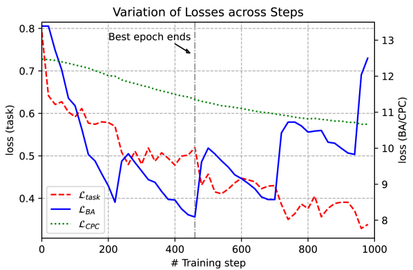
Figure 2: Visualization of loss changing as training proceeds on CMU-MOSEI.

	Text	Visual	Acoustic	$s_{zt}/s_{zv}/s_{za}$	Pred	Truth
(A)	We’ll pick it up from here in the next video in this series.	Smile	Slightly rising tone Normal volume	$0.67/\textbf{0.96}/0.43$	$+0.6663$	$+0.6667$
(B)	I’d probably only give it a two out of five stars.	Frown	Peaceful tone Normal volume	$\textbf{0.85}/\textbf{0.96}/0.36$	$-1.6642$	$-1.6667$
(C)	So these people are commissioned to hunt the animals	Glance	Peaceful & Narrative	$0.64/\textbf{0.93}/0.73$	$-0.0009$	$0.0000$
(D)	I’m sorry, on the scale of one to five I would give this a five.	Turn head	High pitch on “five”	$\textbf{0.83}/0.71/0.54$	$-2.0023$	$+2.6667$

Table 5: Representative examples with their predictions and fusion-modality scores in the case study. High scores ($\geq 0.8$) are highlighted in bold.

5.1 Tracing the Losses

To better understand how MI losses work, we visualize the variation of all losses during training in Figure 2. The values for plotting are the average losses in a constant interval of every 20 steps. From the figure, we can see throughout the training process, $\mathcal{L}_{task}$ and $\mathcal{L}_{CPC}$ keep decreasing nearly all the time, while $\mathcal{L}_{BA}$ goes down in an epoch except the beginning of that. We also mark the time that the best epoch ends, i.e., the task loss on the validation set reaches the minimum. It is notable that $\mathcal{L}_{BA}$ and $\mathcal{L}_{CPC}$ reach a relatively lower level at this time while the task loss on the training set does not. This scenario reveals the crucial role that $\mathcal{L}_{BA}$ and $\mathcal{L}_{CPC}$ play in the training process—they offer supplemental unsupervised gradient rectification to the parameters in their respective back-propagation path and fix up the over-fitting of the task loss. Besides, because in the experiment settings $\alpha$ and $\beta$ are in the same order and at the end of best epoch $\mathcal{L}_{BA}$ reaches the lowest value, which is synchronized as the validation loss, but $\mathcal{L}_{CPC}$ fails to, we can conclude that $\mathcal{L}_{BA}$, or MI maximization in the input (lower) level, has a more significant impact on model’s performance than $\mathcal{L}_{CPC}$, or MI maximization in the fusion (higher) level.

5.2 Case Study

We display some predictions and truth values, as well as corresponding input raw data (for visual and acoustic we only illustrate literally) and three CPC scores in Table 5. As described in Section 3.5, these scores imply how much the fusion results depend on each modality. It is noted that the scores are all beyond 0.35 in all cases, which demonstrates the fusion results seize a certain amount of domain-invariant features. We also observe the different extents that the fusion results depend on each modality. In case (A), visual provides the only clue of the truth sentiment, and correspondingly $s_{zv}$ is higher than the other two scores. In case (B), the word “only” is a piece of additional evidence apart from what visual modality exposes, and we find $s_{zt}$ achieves a higher level than in (A). For (C), acoustic and visual help infer a neutral sentiment and thus $s_{zv}$ and $s_{za}$ are large than $s_{zt}$. Therefore, we conclude that the model can intelligently adjust the information that flows from unimodal input into the fusion results consistently with their individual contribution to the final predictions. However, this mechanism may malfunction in cases like (D). The remark “I’m sorry” bewilders the model and meanwhile visual and acoustic remind none. In this circumstance, the model casts attention on text and is misled to a wrong prediction in the opposite direction.

6 Conclusion

In this paper, we present MMIM, which hierarchically maximizes the mutual information (MI) in a multimodal fusion pipeline. The model applies two MI lower bounds for unimodal inputs and the fusion stage, respectively. To address the intractability of some terms in these lower bounds, we specifically design precise, fast and robust estimation methods to ensure the training can go on normally as well as improve the test outcome. Then we conduct comprehensive experiments on two datasets followed by the ablation study, the results of which verify the efficacy of our model and the necessity of the MI maximization framework. We further visualize the losses and display some representative examples to provide a deeper insight into our model. We believe this work can inspire the creativity in representation learning and multimodal sentiment analysis in the future.

Appendix A Appendix

A.1 Implementation details of history memory

The workflow of the history embedding memory comprises two stages, as shown in Figure 3. In the estimation stage, parameters of the GMM model is estimated using both history embeddings readout from history memory and current batch input, as shown in (a). Then in the update stage, the oldest batch of data is driven out of the memory to leave space for new data, as described in (b). The memory is implemented as a FIFO queue.

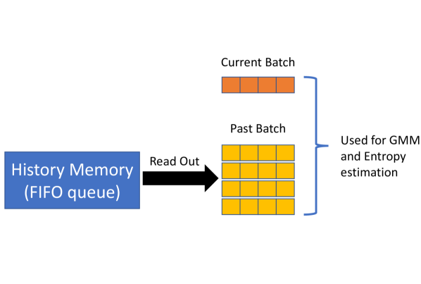
(a)

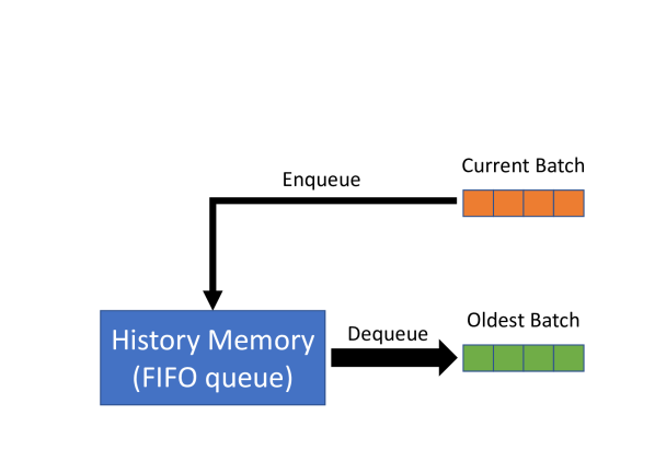
(b)

Figure 3: The workflow of a history embedding memory

A.2 Proof of eq. (7)

Proof.

For a GMM model, the marginal probability density function of $x$ can be written as

$$f(x)=\sum_{i}f(x|z=i)p(x\in C_{i})$$ (15)

where $z$ is an indicator that reflects which class $x$ falls in and $C_{i}$ is the $i^{th}$ class. Since $\sum_{i}P(x\in C_{i})=1$ by Jensen’s inequality we have (note $H(X)=\int(-p(x)\log p(x))dx=\int g(x)dx$ and $g(x)$ is a convex function)

$$\begin{split}H(X)&=H\left(\sum_{i}f(x|z=i)p(x\in C_{i})\right)\\ &\geq\sum_{i}p(x\in C_{i})H(f(x|z=i))\end{split}$$ (16)

In our case we have $p(x\in C_{1})=p(x\in C_{2})=\frac{1}{2}$, then

$$\begin{split}H(X)&\geq\frac{1}{2}\left(H(X;\bm{\mu}_{1},\bm{\Sigma}_{1})+H(X;\bm{\mu}_{2},\bm{\Sigma}_{2})\right)\\ &=K_{L}(X)\end{split}$$ (17)

Hence we get a lower bound of $H(X)$ as the right side of the inequality. On the other hand, an upper bound as proposed in Huber et al. (2008) is

$$\begin{split}K_{U}(X)&=-2\times\frac{1}{2}\times\log\frac{1}{2}+\\ &\frac{1}{2}\left(H(X;\bm{\mu}_{1},\bm{\Sigma}_{1})+H(X;\bm{\mu}_{2},\bm{\Sigma}_{2})\right)\\ &=0.693+K_{L}(X)\end{split}$$ (18)

To summarize

$$K_{L}(X)\leq H(X)\leq K_{U}(X)=0.693+K_{L}(X)$$ (19)

Then through maximizing the lower bound $K_{L}(X)$ we can maximize $H(X)$. ∎

References

- Akhtar et al. (2019) Md Shad Akhtar, Dushyant Chauhan, Deepanway Ghosal, Soujanya Poria, Asif Ekbal, and Pushpak Bhattacharyya. 2019. Multi-task learning for multi-modal emotion recognition and sentiment analysis. In Proceedings of the 2019 Conference of the North American Chapter of the Association for Computational Linguistics: Human Language Technologies, Volume 1 (Long and Short Papers), pages 370–379.
- Alemi et al. (2016) Alexander A Alemi, Ian Fischer, Joshua V Dillon, and Kevin Murphy. 2016. Deep variational information bottleneck. arXiv preprint arXiv:1612.00410.
- Amjad and Geiger (2019) Rana Ali Amjad and Bernhard C Geiger. 2019. Learning representations for neural network-based classification using the information bottleneck principle. IEEE transactions on pattern analysis and machine intelligence, 42(9):2225–2239.
- Arandjelovic and Zisserman (2017) Relja Arandjelovic and Andrew Zisserman. 2017. Look, listen and learn. In Proceedings of the IEEE International Conference on Computer Vision, pages 609–617.
- Bachman et al. (2019) Philip Bachman, R Devon Hjelm, and William Buchwalter. 2019. Learning representations by maximizing mutual information across views. arXiv preprint arXiv:1906.00910.
- Barber and Agakov (2004) David Barber and Felix Agakov. 2004. The IM algorithm: A variational approach to information maximization. Advances in neural information processing systems, 16:201.
- Belghazi et al. (2018) Mohamed Ishmael Belghazi, Aristide Baratin, Sai Rajeshwar, Sherjil Ozair, Yoshua Bengio, Aaron Courville, and Devon Hjelm. 2018. Mutual information neural estimation. In International Conference on Machine Learning, pages 531–540. PMLR.
- Chen et al. (2017) Minghai Chen, Sen Wang, Paul Pu Liang, Tadas Baltrušaitis, Amir Zadeh, and Louis-Philippe Morency. 2017. Multimodal sentiment analysis with word-level fusion and reinforcement learning. In Proceedings of the 19th ACM International Conference on Multimodal Interaction, pages 163–171.
- Cheng et al. (2020) Pengyu Cheng, Weituo Hao, Shuyang Dai, Jiachang Liu, Zhe Gan, and Lawrence Carin. 2020. Club: A contrastive log-ratio upper bound of mutual information. In International Conference on Machine Learning, pages 1779–1788. PMLR.
- Degottex et al. (2014) Gilles Degottex, John Kane, Thomas Drugman, Tuomo Raitio, and Stefan Scherer. 2014. Covarep—a collaborative voice analysis repository for speech technologies. In 2014 ieee international conference on acoustics, speech and signal processing (icassp), pages 960–964. IEEE.
- Deonna and Teroni (2012) Julien Deonna and Fabrice Teroni. 2012. The emotions: A philosophical introduction. Routledge.
- Devlin et al. (2019) Jacob Devlin, Ming-Wei Chang, Kenton Lee, and Kristina Toutanova. 2019. Bert: Pre-training of deep bidirectional transformers for language understanding. In Proceedings of the 2019 Conference of the North American Chapter of the Association for Computational Linguistics: Human Language Technologies, Volume 1 (Long and Short Papers), pages 4171–4186.
- Ghosal et al. (2019) Deepanway Ghosal, Navonil Majumder, Soujanya Poria, Niyati Chhaya, and Alexander Gelbukh. 2019. DialogueGCN: A graph convolutional neural network for emotion recognition in conversation. In Proceedings of the 2019 Conference on Empirical Methods in Natural Language Processing and the 9th International Joint Conference on Natural Language Processing (EMNLP-IJCNLP), pages 154–164, Hong Kong, China. Association for Computational Linguistics.
- Gutmann and Hyvärinen (2010) Michael Gutmann and Aapo Hyvärinen. 2010. Noise-contrastive estimation: A new estimation principle for unnormalized statistical models. In Proceedings of the Thirteenth International Conference on Artificial Intelligence and Statistics, pages 297–304. JMLR Workshop and Conference Proceedings.
- Hazarika et al. (2018) Devamanyu Hazarika, Soujanya Poria, Sruthi Gorantla, Erik Cambria, Roger Zimmermann, and Rada Mihalcea. 2018. CASCADE: Contextual sarcasm detection in online discussion forums. In Proceedings of the 27th International Conference on Computational Linguistics, pages 1837–1848.
- Hazarika et al. (2020) Devamanyu Hazarika, Roger Zimmermann, and Soujanya Poria. 2020. MISA: Modality-invariant and-specific representations for multimodal sentiment analysis. In Proceedings of the 28th ACM International Conference on Multimedia, pages 1122–1131.
- He et al. (2020) Kaiming He, Haoqi Fan, Yuxin Wu, Saining Xie, and Ross Girshick. 2020. Momentum contrast for unsupervised visual representation learning. In Proceedings of the IEEE/CVF Conference on Computer Vision and Pattern Recognition, pages 9729–9738.
- Hjelm et al. (2018) R Devon Hjelm, Alex Fedorov, Samuel Lavoie-Marchildon, Karan Grewal, Phil Bachman, Adam Trischler, and Yoshua Bengio. 2018. Learning deep representations by mutual information estimation and maximization. In International Conference on Learning Representations.
- Hochreiter and Schmidhuber (1997) Sepp Hochreiter and Jürgen Schmidhuber. 1997. Long short-term memory. Neural computation, 9(8):1735–1780.
- Huber et al. (2008) Marco F Huber, Tim Bailey, Hugh Durrant-Whyte, and Uwe D Hanebeck. 2008. On entropy approximation for gaussian mixture random vectors. In 2008 IEEE International Conference on Multisensor Fusion and Integration for Intelligent Systems, pages 181–188. IEEE.
- Kerroum et al. (2010) Mounir Ait Kerroum, Ahmed Hammouch, and Driss Aboutajdine. 2010. Textural feature selection by joint mutual information based on gaussian mixture model for multispectral image classification. Pattern Recognition Letters, 31(10):1168–1174.
- Liu et al. (2018) Zhun Liu, Ying Shen, Varun Bharadhwaj Lakshminarasimhan, Paul Pu Liang, AmirAli Bagher Zadeh, and Louis-Philippe Morency. 2018. Efficient low-rank multimodal fusion with modality-specific factors. In Proceedings of the 56th Annual Meeting of the Association for Computational Linguistics (Volume 1: Long Papers), pages 2247–2256.
- Mai et al. (2020) Sijie Mai, Haifeng Hu, and Songlong Xing. 2020. Modality to modality translation: An adversarial representation learning and graph fusion network for multimodal fusion. In Proceedings of the AAAI Conference on Artificial Intelligence, volume 34, pages 164–172.
- Melville et al. (2009) Prem Melville, Wojciech Gryc, and Richard D Lawrence. 2009. Sentiment analysis of blogs by combining lexical knowledge with text classification. In Proceedings of the 15th ACM SIGKDD international conference on Knowledge discovery and data mining, pages 1275–1284.
- Morency et al. (2011) Louis-Philippe Morency, Rada Mihalcea, and Payal Doshi. 2011. Towards multimodal sentiment analysis: Harvesting opinions from the web. In Proceedings of the 13th international conference on multimodal interfaces, pages 169–176.
- Ngiam et al. (2011) Jiquan Ngiam, Aditya Khosla, Mingyu Kim, Juhan Nam, Honglak Lee, and Andrew Y Ng. 2011. Multimodal deep learning. In ICML.
- Nilsson et al. (2002) Mattias Nilsson, Harald Gustaftson, Søren Vang Andersen, and W Bastiaan Kleijn. 2002. Gaussian mixture model based mutual information estimation between frequency bands in speech. In 2002 IEEE International Conference on Acoustics, Speech, and Signal Processing, volume 1, pages I–525. IEEE.
- Oord et al. (2018) Aaron van den Oord, Yazhe Li, and Oriol Vinyals. 2018. Representation learning with contrastive predictive coding. arXiv preprint arXiv:1807.03748.
- Pham et al. (2019) Hai Pham, Paul Pu Liang, Thomas Manzini, Louis-Philippe Morency, and Barnabás Póczos. 2019. Found in translation: Learning robust joint representations by cyclic translations between modalities. In Proceedings of the AAAI Conference on Artificial Intelligence, volume 33, pages 6892–6899.
- Poole et al. (2019) Ben Poole, Sherjil Ozair, Aaron Van Den Oord, Alex Alemi, and George Tucker. 2019. On variational bounds of mutual information. In International Conference on Machine Learning, pages 5171–5180. PMLR.
- Poria et al. (2020) Soujanya Poria, Devamanyu Hazarika, Navonil Majumder, and Rada Mihalcea. 2020. Beneath the tip of the iceberg: Current challenges and new directions in sentiment analysis research. IEEE Transactions on Affective Computing, pages 1–1.
- Rahman et al. (2020) Wasifur Rahman, Md Kamrul Hasan, Sangwu Lee, AmirAli Bagher Zadeh, Chengfeng Mao, Louis-Philippe Morency, and Ehsan Hoque. 2020. Integrating multimodal information in large pretrained transformers. In Proceedings of the 58th Annual Meeting of the Association for Computational Linguistics, pages 2359–2369, Online. Association for Computational Linguistics.
- Sun et al. (2020) Zhongkai Sun, Prathusha Sarma, William Sethares, and Yingyu Liang. 2020. Learning relationships between text, audio, and video via deep canonical correlation for multimodal language analysis. In Proceedings of the AAAI Conference on Artificial Intelligence, volume 34, pages 8992–8999.
- Tishby and Zaslavsky (2015) Naftali Tishby and Noga Zaslavsky. 2015. Deep learning and the information bottleneck principle. In 2015 IEEE Information Theory Workshop (ITW), pages 1–5. IEEE.
- Tsai et al. (2019a) Yao-Hung Hubert Tsai, Shaojie Bai, Paul Pu Liang, J Zico Kolter, Louis-Philippe Morency, and Ruslan Salakhutdinov. 2019a. Multimodal Transformer for unaligned multimodal language sequences. In Proceedings of the Annual Meeting of the Association for Computational Linguistics.
- Tsai et al. (2019b) Yao-Hung Hubert Tsai, Paul Pu Liang, Amir Zadeh, Louis-Philippe Morency, and Ruslan Salakhutdinov. 2019b. Learning factorized multimodal representations. In International Conference on Representation Learning.
- Tsai et al. (2020) Yao-Hung Hubert Tsai, Martin Ma, Muqiao Yang, Ruslan Salakhutdinov, and Louis-Philippe Morency. 2020. Multimodal routing: Improving local and global interpretability of multimodal language analysis. In Proceedings of the 2020 Conference on Empirical Methods in Natural Language Processing (EMNLP), pages 1823–1833.
- Veličković et al. (2018) Petar Veličković, William Fedus, William L Hamilton, Pietro Liò, Yoshua Bengio, and R Devon Hjelm. 2018. Deep graph infomax. In International Conference on Learning Representations.
- Wang et al. (2017) Haohan Wang, Aaksha Meghawat, Louis-Philippe Morency, and Eric P Xing. 2017. Select-additive learning: Improving generalization in multimodal sentiment analysis. In 2017 IEEE International Conference on Multimedia and Expo (ICME), pages 949–954. IEEE.
- Wöllmer et al. (2013) Martin Wöllmer, Felix Weninger, Tobias Knaup, Björn Schuller, Congkai Sun, Kenji Sagae, and Louis-Philippe Morency. 2013. Youtube movie reviews: Sentiment analysis in an audio-visual context. IEEE Intelligent Systems, 28(3):46–53.
- Yu et al. (2021) Wenmeng Yu, Hua Xu, Ziqi Yuan, and Jiele Wu. 2021. Learning modality-specific representations with self-supervised multi-task learning for multimodal sentiment analysis. arXiv preprint arXiv:2102.04830.
- Yuan and Liberman (2008) Jiahong Yuan and Mark Liberman. 2008. Speaker identification on the scotus corpus. The Journal of the Acoustical Society of America, 123(5):3878–3878.
- Zadeh et al. (2017) Amir Zadeh, Minghai Chen, Soujanya Poria, Erik Cambria, and Louis-Philippe Morency. 2017. Tensor fusion network for multimodal sentiment analysis. In Proceedings of the 2017 Conference on Empirical Methods in Natural Language Processing, pages 1103–1114.
- Zadeh et al. (2016) Amir Zadeh, Rowan Zellers, Eli Pincus, and Louis-Philippe Morency. 2016. Multimodal sentiment intensity analysis in videos: Facial gestures and verbal messages. IEEE Intelligent Systems, 31(6):82–88.
- Zadeh et al. (2018) AmirAli Bagher Zadeh, Paul Pu Liang, Soujanya Poria, Erik Cambria, and Louis-Philippe Morency. 2018. Multimodal language analysis in the wild: CMU-MOSEI dataset and interpretable dynamic fusion graph. In Proceedings of the 56th Annual Meeting of the Association for Computational Linguistics (Volume 1: Long Papers), pages 2236–2246.