Inferring gene regulation dynamics from static snapshots of gene expression variability

Abstract

Inferring functional relationships within complex networks from static snapshots of a subset of variables is a ubiquitous problem in science. For example, a key challenge of systems biology is to translate cellular heterogeneity data obtained from single-cell sequencing or flow-cytometry experiments into regulatory dynamics. We show how static population snapshots of co-variability can be exploited to rigorously infer properties of gene expression dynamics when gene expression reporters probe their upstream dynamics on separate time-scales. This can be experimentally exploited in dual-reporter experiments with fluorescent proteins of unequal maturation times, thus turning an experimental bug into an analysis feature. We derive correlation conditions that detect the presence of closed-loop feedback regulation in gene regulatory networks. Furthermore, we show how genes with cell-cycle dependent transcription rates can be identified from the variability of co-regulated fluorescent proteins. Similar correlation constraints might prove useful in other areas of science in which static correlation snapshots are used to infer causal connections between dynamically interacting components.

I Introduction

A large body of experimental work has quantified significant non-genetic variability in living cells [1, 2, 3, 4, 5, 6, 7, 8]. Harnessing the information contained in this naturally occurring variability to infer molecular processes in cells without perturbation experiments is a long-standing goal of systems biology. However, measuring the spontaneous non-genetic variability of only one cellular component does not have sufficient discriminatory power to distinguish between models of complex cellular processes with many interacting components [9]. Fortunately, progress in experimental techniques has made it possible to measure multiple components simultaneously. For example, covariances between mRNA and protein levels have been used to test hypotheses about translation rates in bacteria [10].

Despite improvements in experimental methods, it remains technically challenging to measure multiple different types of molecules in the same cell. More feasible, and thus more common, are experiments that measure multiple levels of the same type of molecule, e.g., measuring different mRNA levels using sequencing techniques [11], or measuring abundances of proteins using fluorescence microscopy [12]. Such experiments have motivated “dual reporter” approaches in which correlations between identical copies of reporters responding to a common upstream signal are used to characterize sources of variability within cellular processes [12, 13, 14].

Previous work focused on splitting the total observed variability into “intrinsic” and “extrinsic” contributions under the assumption that reporters are identical in all intrinsic properties. However, actual experimental reporters are never exactly identical. For example, commonly used fluorescent proteins differ enormously in their maturation half-lifes ranging from minutes to hours [15]. We show that despite such asymmetries, gene expression reporters can be used to rigorously detect closed-loop control networks from correlation measurements. Furthermore, we show that the inherent asymmetry of reporters can in fact be exploited to our advantage. Because reporters that differ in their intrinsic dynamics respond to their shared upstream input on different time-scales, their variability contains information about the unobserved upstream dynamics even when we have only access to static population snapshots. For example, we show how asymmetric dual reporters can be used to distinguish periodically varying deterministic driving from stochastic upstream “noise”.

The utility of these results lies in interpreting experimental data even when only a small part of a complex regulatory process can be observed directly. Instead of trying to model all of the many direct and indirect steps of gene expression regulation, we analyze entire classes of systems in which we specify only some steps but leave all other details unspecified. This approach allows us to derive inequalities that constrain the space of behaviour that could possibly be observed across a population of genetically identical cells within these classes, regardless of the details of the unspecified parts. These inequalities are in terms of coefficients of variation (CVs) and correlation coefficients of reporter levels, $x$ and $y$, engineered to readout components-of-interest,

$$CV_{x}:=\frac{\sqrt{\mathrm{Var}(x)}}{\langle x\rangle}\quad\rho_{xy}:=\frac{\mathrm{Cov}(x,y)}{\sqrt{\mathrm{Var}(x)\mathrm{Var}(y)}}$$

where angular brackets denote population averages. Such population statistics are experimentally accessible from static snapshots of cellular populations that have reached a time-independent distribution of cell-to-cell variability. If a measurement violates our inequalities, one of our assumptions must be false, regardless of how the unspecified part of the system behaves. This way mathematical constraints can be used to deduce features of gene expression.

While our results are motivated by methods in experimental cell biology to understand gene expression dynamics, they apply to any “reporters” embedded in a dynamic interaction network, subject to the specified production and elimination fluxes considered here and may thus be more broadly applicable.

II Detecting gene regulation feedback from static snapshots of population heterogeneity

Cells employ both open-loop regulation or closed-loop feedback to control cellular processes [16]. Here we show how to infer the presence of closed-loop feedback for any molecule within a network, by introducing an additional reporter molecule into the system. After describing the key theoretical result we detail the experimental set-up to detect feedback control in gene regulation from mRNA levels or fluorescent protein measurements. In brief, our results apply to “dual reporter” genes that are engineered to share an unspecified but identical transcription rate. This assumption defines our class of models and needs to be experimentally ensured through appropriate genetic engineering in combination with self-consistency checks, such as indistinguishable reporter distributions, as for example reported in [13, 4, 12, 17]. Further experimental considerations are discussed in Sec. IV.

II.1 Mathematical correlation constraints for open-loop “dual reporters”

Motivated by the transcriptional dynamics of co-regulated genes, we consider a generic class of systems in which two cellular components, X and Y, are produced with a common (but unspecified) time-varying rate, and are degraded in a first order reaction, with average life-times $\tau_{x}$ and $\tau_{y}$, respectively

$$\vspace{-.8ex}x \xrightarrow{\mathmakebox{R(\mathbf{u}(t))}}x+1\qquad y\xrightarrow{\mathmakebox{R(\mathbf{u}(t))}}y+1$$

$$x \xrightarrow{\mathmakebox{x/\tau_{x}}}x-1\qquad y\xrightarrow{\mathmakebox{y/\tau_{y}}}y-1\vspace{-.8ex}$$ (1)

where the transcription rate can depend in any way on a cloud of unknown components $\mathbf{u}(t)$, which in turn can depend in arbitrary ways on the number of X and Y molecules, denoted by $x$ and $y$. While we characterize the stochastic reactions of X and Y, the dynamics of all other cellular components remain unspecified, see Fig. 1A, and the resulting dynamics need not be Markovian or ergodic in X and Y. A related class of stochastic processes has been previously considered to analyze mRNA-protein correlations in gene expression [9], whereas here we analyze correlations between co-regulated transcripts.

Previous work established universal probability balance relations that constrain the stationary state distributions of stochastic processes [18]. For the above class of systems, these relations translate the specified reactions of Eq. (1) into an underdetermined system of equations for (co)variances (see Appendix A). Though this system of equations cannot be solved due to the unspecified parts of the dynamics, not all dual reporter correlations $\rho_{xy}$ are accessible for all variability ratios $CV_{x}/CV_{y}$. For example, the correlation of any system is bounded by the correlation of two reporters that respond deterministically to their upstream input (Appendix A). When the two reporters respond to their upstream input on unequal timescales, their correlations are constrained as illustrated by the dashed orange lines in Fig. 1B that bound all systems for a given value of $T:=\tau_{y}/\tau_{x}$. In Fig. 1 and throughout the paper, numerical simulations of specific stochastic models and parameters establish that the inequalities are tight, i.e., that the entire bounded regions are accessible. For illustration, we plot a subset of simulations with arbitrarily chosen sampling density, along with the analytically proven constraints.

The space of possible correlations is restricted much further for open-loop systems in which upstream variables regulate the reporter production rates but are not affected by them, corresponding to all possible systems in Fig. 1A in which X and Y do not affect the unspecified cloud. For all such systems, we can derive additional constraints by considering the hypothetical average of an ensemble of stochastic dual reporters conditioned on the history of their upstream influences. While these conditional averages are typically experimentally inaccessible, they mathematically constrain the measurable (co)variances. We find (see Appendix B) that the correlations of cellular components X and Y that are regulated through an open-loop process must satisfy

$$\frac{\Big{|}\dfrac{CV_{x}}{CV_{y}}-T\dfrac{CV_{y}}{CV_{x}}\Big{|}}{1-T}\leqslant\rho_{xy}\quad\text{with}\quad T:=\tau_{y}/\tau_{x},$$ (2)

where without loss of generality we assume that $T\leqslant 1$, i.e., that Y is the faster reporter. Fig. 1B shows the above “open-loop constraint” of Eq. (2) as solid orange lines, for specific values of $T$. Note that, in the symmetric limit $T\to 1$, Eq. (2) reduces to $\rho_{xy}\geqslant 0$ and $CV_{x}=CV_{y}$ as intuitively expected.

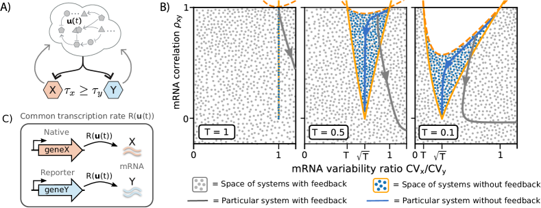
Figure 1: Feedback in gene regulation affects the space of possible mRNA covariability. A) We consider all stochastic processes in which two components, X and Y, are made with an identical, but unspecified, rate. This rate can depend in any way on a cloud of unknown components $\mathbf{u}(t)$, which in turn can depend in arbitrary ways on the number of X and Y molecules. The shared production rate of X and Y, together with first-order degradation of X and Y with respective lifetimes $\tau_{x}$ and $\tau_{y}$, are the only specified parts within this arbitrarily large network, as defined in Eq. (1). B) Space of possible covariability for different values of the life-time ratio $T:=\tau_{y}/\tau_{x}$. All systems must satisfy $\rho_{xy}(1+T)\leqslant CV_{x}/CV_{y}+TCV_{y}/CV_{x}$ corresponding to the area below the dashed orange line. Allowing for feedback (grey dots), the entire space below the dashed orange line is accessible. In the absence of feedback (blue dots), $\rho_{xy}$ is additionally constrained by Eq. (2), corresponding to the region between the solid orange lines. Dots are stochastic simulation data for specific models of co-regulated genes within the class defined in Eq. (1). Plotted are a subset of simulations with arbitrary density to demonstrate the accessibility of the constrained regions. Blue and grey curves are exemplary toy models (Appendix G) that illustrate the effect of decreasing transcription rate variability (blue) or increasing feedback strength (grey). C) Experimental set-up to detect feedback in the regulation of a native gene of interest geneX. The native and reporter genes are regulated by identical promoters in the same cell. If the covariability of the transcripts X and Y of such genes falls outside the open-loop constraint of Eq. (2), we can conclude that the gene of interest geneX regulates its own transcription. To maximize the discriminatory power of the approach the reporter geneY should be engineered to be a passive read-out of transcription without significantly affecting gene expression.

Any system whose measured (co)variability falls outside the region defined by Eq. (2) must be regulated through closed-loop feedback. Violations of this constraint can thus be used to experimentally detect the presence of feedback based on static population variability measurements without the need for perturbations. Fig. 1B shows the (co)variability of simulated systems with feedback (grey dots) and without feedback (blue dots), illustrating that only systems with feedback can fall outside the region bounded by solid orange lines, violating the “open-loop constraint” of Eq. (2). The position of a system outside the “open-loop constraint” can be used to quantify a heuristic “feedback strength” and provides additional information to distinguish positive from negative feedback (see Appendix B.2).

II.2 Experimentally exploiting mRNA correlations to detect feedback

Eq. (2) can be exploited through an experimental set-up analogous to previously engineered circuits in which co-regulated genes reportedly satisfied the assumptions of Eq. (1) and transcripts were counted with single molecule fluorescence in-situ hybridization (smFISH) [17, 19]. To detect feedback regulation of a gene of interest geneX, a reporter geneY should be introduced whose expression is under the control of an identical copy of the promoter of geneX, see Fig. 1C. The precise sequence of the reporter gene is unimportant as long as its transcript Y is sufficiently different from the transcript X of the gene of interest to avoid cross-hybridization by RNA probes. This can be achieved, e.g., by making the reporter gene sequence a scrambled version of the gene of interest.

Using smFISH, transcripts X and Y can be measured simultaneously at the single cell level [20]. Simple population snapshots of cell-to-cell variability then determine whether experimentally observed $CV_{x}$, $CV_{y}$, $\rho_{xy}$ violate Eq. (2). If this open-loop constraint is violated we can conclude that geneX must directly or indirectly affect its own production rate.

If a system falls inside the region defined by Eq. (2) we cannot say whether it is regulated through feedback or not, see Fig. 1B. That is because systems with infinitesimally weak feedback are fundamentally indistinguishable from open-loop processes. To detect significant feedback in geneX, it is advantageous to ensure the reporter geneY is not involved in the same feedback regulation. This could, e.g., be achieved by removing the start codon from geneY so its mRNA is not translated, thus preventing the protein of geneY from exerting any feedback control. Furthermore, by ensuring that the life-time of the second reporter transcript is comparable to that of the gene of interest we can minimize the accessible area defined by Eq. (2) and thus maximize the discriminatory power of the approach.

Note that only relative abundances are necessary to determine $CV_{x}$, $CV_{y}$, and $\rho_{xy}$. The above steps can thus be applied to data from single cell sequencing techniques. Additionally, severe violations of Eq. (2) can potentially be detected already from sequential rather than simultaneous measurements of X and Y: if their ratio of CVs falls outside the interval $[T,1]$ then Eq. (2) must be violated regardless of the value of $\rho_{xy}$. When analyzing genes with potentially unknown mRNA life-time, the ratio of mRNA life-times $T$ can be inferred from pairwise correlation measurements between three reporter genes, as detailed in Sec. IV.

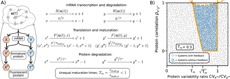
Figure 2: Feedback in gene regulation affects the possible covariability of fluorescent protein measurements. A) As before X and Y correspond to co-regulated mRNA, but we now explicitly include the dynamics of immature fluorescent proteins denoted as X’ and Y’, as well as mature fluorescent proteins X” and Y”. Because fluorescent proteins are typically stable and are thus effectively diluted with a common “degradation” time set by the cell-cycle, we focus on gene expression dynamics that is symmetric apart from the maturation step. The asymmetry between the co-regulated genes is then entirely characterized by the ratio of average fluorescent maturation times $T_{\mathrm{m}}:=\tau_{\mathrm{mat},y}/\tau_{\mathrm{mat},x}$. B) Without feedback control (blue dots), fluorescence correlations are constrained to the region between the dashed and solid orange lines, the latter corresponding to the bound of Eq. (3). Allowing for feedback (grey dots), the entire region becomes available. Correlations in fluorescence levels can thus be used to detect causal feedback in gene regulation from static population snapshots. Dots are selected numerical simulations of specific fluorescent reporter systems within this class that illustrate the full accessibility of the region constrained by the analytically proven bounds.

II.3 Experimentally exploiting fluorescent protein correlations to detect feedback

Similar constraints can be derived to interpret gene expression data in which fluorescent fusion proteins are used to quantify gene expression [4]. In this case the experimental read-out involves a fluorescent maturation step in addition to transcription and translation. While this maturation step is often well approximated as exponential [15], its life-time differs significantly between commonly used fluorescent proteins. For example, the maturation half-lifes of mCerulean, mEYFP, mEGFP, and mRFP1 are 6.6 min, 9 min, 14.5 min and 21.9 min respectively [15]. In order to detect gene regulatory feedback from (co)variability data in such an experimental set-up, we extend our previous class of systems to explicitly account for protein translation and maturation events, see Fig. 2A. In this parallel cascade system X^′′ and Y^′′ represent the level of mature fluorescent proteins.

Crucially, open-loop systems in which none of the gene products directly, or indirectly, affect their transcription rate must additionally satisfy

$$\text{max}\left(\frac{T_{m}\mfrac{CV_{y^{\prime\prime}}}{CV_{x^{\prime\prime}}}-\mfrac{CV_{x^{\prime\prime}}}{CV_{y^{\prime\prime}}}}{1-T_{m}},0\right)\leqslant\rho_{x^{\prime\prime}y^{\prime\prime}}\hskip 5.60002pt\text{\&}\hskip 6.02pt\frac{CV_{x^{\prime\prime}}}{CV_{y^{\prime\prime}}}\leqslant 1,$$ (3)

where $T_{\mathrm{m}}:=\tau_{\mathrm{mat},y}/\tau_{\mathrm{mat},x}$ is the ratio of maturation times between the two fluorescent proteins (see Appendix E). The “left boundary” of this region is mathematically identical to the previous bound of Eq. (2), but now applied to the statistics of fluorescence levels X^′′ and Y^′′. The new right-hand bound $CV_{x^{\prime\prime}}\leqslant CV_{y^{\prime\prime}}$ broadens the region accessible to open-loop processes due the additional intrinsic degrees of freedom of this class of systems. Fig. 2B illustrates the tightness of these bounds (solid orange lines) for $T_{m}=0.5$, where dots correspond to simulated systems with (grey) and without feedback (blue).

Moreover, analogously to the mRNA-correlations, all possible fluorescence correlations for open-loop systems are constrained by $\rho_{x^{\prime\prime}y^{\prime\prime}}(1+T_{m})\leqslant T_{m}CV_{x^{\prime\prime}}/CV_{y^{\prime\prime}}+T_{m}CV_{y^{\prime\prime}}/CV_{x^{\prime\prime}}$. Correlations of systems with feedback can break this bound, as shown by the grey dots in Fig. 2B. This is because in the limit of infinitesimally small maturation times and mRNA fluctuations, the system becomes identical to Fig. 1A with $T=1$, which has unbounded correlations as shown in Fig. 1B.

Fluorescent proteins can thus be used to detect whether a given gene regulates its own production as follows. Considering geneZ as the native gene of interest, two recombinant genes, geneZ-GFP and geneZ-RFP (or other spectrally distinguishable pairs) would be engineered into an isogenic cell population under the control of the same (but distinct) promoter as geneZ. The transcripts of geneZ-GFP and geneZ-RFP then correspond to X and Y in Fig. 2A, as they are transcribed with identical rates. The level of mature fusion protein, X^′′ and Y^′′, can be read out at the single-cell level with fluorescence microscopy, and from the observed $CV_{x^{\prime\prime}}$, $CV_{y^{\prime\prime}}$, and $\rho_{x^{\prime\prime}y^{\prime\prime}}$ we can detect violations of the open-loop constraint Eq. (3).

If necessary, the discriminatory power of this approach can be increased by introducing a third fusion protein with a different fluorescent maturation time to eliminate the unknown internal degrees of freedom, and determine how much variability is generated through transcriptional, translational, or maturation events (see Appendix J.3).

In modeling this parallel cascade system, we assumed the gene expression dynamics of the two fusion proteins is identical apart from the fluorescent maturation step. This is motivated by the experimental set-up in which we use the same native protein fused to two different fluorescent proteins. The absence of further asymmetries, e.g., caused by codon usage, translation initiation, or reporter cross talk, would need to be established experimentally. Traditionally, this has been done by comparing the distributions of reporter variability for reporters that are claimed to be identical in their transcriptional and translational dynamics [13, 4, 12, 17]. Note that the class of systems defined in Fig. 2A is in fact a subset of a much larger class of systems in which the key specified part is that there is a final maturation step in a symmetric but otherwise unspecified intrinsic cascade of arbitrary steps (see Appendix D), thus allowing for a cascade of sequential post translational modifications that occur before the maturation step.

So far we considered arbitrary values of $T$ to allow for the experimental reality that reporters are never completely identical. Our next results show that $T\neq 1$ is not just a nuisance but can be exploited to infer the dynamics of the transcription rate of open-loop systems.

III Distinguishing stochastic from deterministic transcription rate variability

[capbesideposition=right,bottom,capbesidewidth=0.42]figure

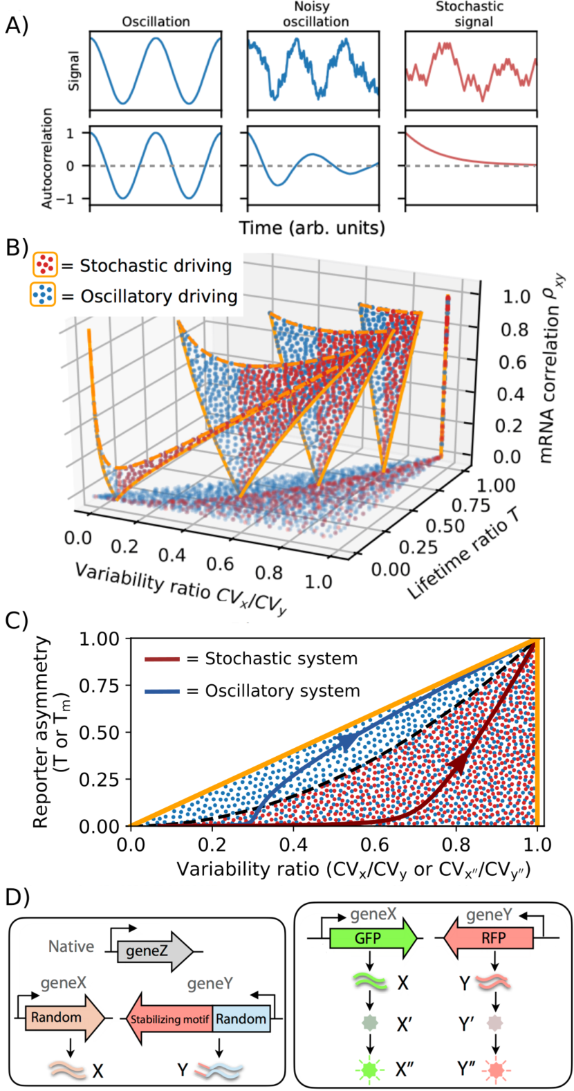
Figure 3: Periodic transcriptional variability can be distinguished from stochastic variability without experimental access to transcription rates and without following individual cells over time. A) In a noisy cellular milieu, the auto-correlation of a periodic signal is not perfectly periodic but decays. We thus operationally define a signal as periodic when its periodicity is strong enough such that its auto-correlation function becomes negative at some point. Conversely, we classify signals with non-negative auto-correlations as stochastic. B) The left-side of the “open-loop” region defined by Eq. (2) is only accessible by mRNA reporters that are driven by oscillatory production rates rather than purely stochastic upstream variability. The boundary (dashed black) line is defined by Eq. (4). C) Sequential measurements of mRNA reporters X and Y, or fluorescent proteins X” and Y”, can be used to discriminate between stochastic and oscillatory transcription rates if a system violates the respective bounds of Eq. (4) or Eq. (5) (indicated by dashed black line). Selected numerical simulation (dots) illustrate the achievability of the constrained regions, and the arrowed curves indicate how specific models (Appendix G) behave as the downstream response becomes slower. For these systems, we find that oscillatory systems cross the black dashed line when $2\pi\sqrt{\tau_{x}\tau_{y}}$ or $2\pi\sqrt{\tau_{\mathrm{mat},x}\tau_{\mathrm{mat},y}}$ become slower than the period of the driving oscillation. To detect oscillations it is thus advantageous to choose slow reporters. D) Periodic transcription rates of a gene of interest geneZ can be experimentally detected either utilizing mRNA reporters, X and Y (left panel), or fluorescent protein reporters, X” and Y” (right panel), driven by the promoter of geneZ. If experimental reporters violate Eq. (4) or (5), they land to the left of the dashed black line (panel C), and geneZ must be driven by a periodically varying transcription rate.

A fundamental issue when interpreting cell-to-cell variability is that we generally do not know whether a component’s variability is due to stochastic upstream noise or whether a component is driven by deterministic variability [21]. Next, we show how we can distinguish the two types of dynamics from static population snapshots of asymmetric gene expression reporters.

III.1 Mathematical correlation constraints for stochastic transcriptional noise

Focusing on the class of systems defined in Eq. (1) in the absence of feedback, we next show how snapshots of dual reporters can be used to infer temporal properties of the unobserved production rates. To discuss periodic driving in cells we consider the stationary state auto-correlation of the transcription rate

$$A(s):=\frac{\langle R(t+s)R(t)\rangle-\langle R(t+s)\rangle\langle R(t)\rangle}{\mathrm{Var}[R(t)]}.$$

We define a production rate as periodic if this auto-correlation $A(s)$ becomes negative for some $s$. In other words, the periodicity of the driving has to be strong enough such that the rate of production is negatively correlated with itself some time later. Conversely, we define upstream variability as stochastic if the auto-correlation of the unobserved transcription rate is non-negative everywhere, see Fig. 3A.

Fourier analysis of the dynamics of X and Y conditioned on the histories of their production rates shows (Appendix C) that not all systems can exhibit fluctuations everywhere within the region defined by Eq. (2). Components that are stochastically driven are additionally constrained by

$$\sqrt{T}\leqslant\frac{CV_{x}}{CV_{y}},$$ (4)

Sequential measurements of $CV_{x}$ and $CV_{y}$ from static snapshots of X and Y can thus discriminate between deterministic and stochastic transcription rates when $CV_{x}<CV_{y}\sqrt{T}$ without access to time-series data or directly measuring the unobserved upstream dynamics. Fig. 3 illustrate this discriminatory power with simulated systems in which genes that are periodically driven (blue dots) can fill the entire region defined by Eq. (2) (solid yellow lines), whereas genes that are driven stochastically (red dots) are further constrained by Eq. (4) (dashed black line).

A pair of asymmetric ($T<1$), co-regulated reporters in an open-loop system can exhibit perfect correlations ($\rho_{xy}=1$) in two distinct regimes, see Fig. 3B. First, when the upstream variability is much slower than both $\tau_{x}$ and $\tau_{y}$, the reporters adjust rapidly to their quasi-stationary states such that $y(t)=Tx(t)$ at all times, and thus $CV_{x}=CV_{y}$. The second regime occurs when production rates oscillates rapidly, such that the upstream signal enslaves the reporters into a transient regime where their different response times simply shift their average dynamics. This second regime is not accessible by reporters that are driven stochastically. Instead, in the limit of infinitely fast stochastic variability, dual reporter systems approach $CV_{x}/CV_{y}\to\sqrt{T}$ corresponding to the bound of Eq. (4). Where on the right-hand side a stochastically driven system falls can be used to infer the time-scale of the upstream fluctuations (Appendix C).

Inferring upstream dynamics from static snapshots is possible because the reporters probe their upstream dynamics on different time-scales. In fact, in the hypothetical limit of an infinite number of reporters responding to an upstream signal on all time-scales, the auto-correlation of the upstream signal is entirely determined by static measurements of its downstream variability. That is because knowing a signal’s downstream variability on all time-scales effectively determines the Laplace transform of its auto-correlation, see Appendix C.

III.2 Experimentally exploiting mRNA correlations to detect periodic transcription rates

The constraint of Eq. (4) can be exploited to detect periodic transcription rates, in experiments in which the promoter of a gene of interest is used to independently drive the expression of two non-native passive gene expression reporters [17, 19]. The details of the two reporter genes are not important as long as their transcripts have unequal life-times, and their products are not involved in any cellular control. Both criteria can be satisfied, e.g., by using a random sequence to encode the first reporter, and combining another random sequence with a mRNA stabilizing motif to encode the second reporter. This motif could be a 5’ stem-loop structure in the case of prokaryotic cells or a carbohydrate recognition domain (CRD) sequence in eukaryotes [22, 23]. Transcript levels of the two reporter genes then correspond to our components X and Y. Fig. 3D (left panel) illustrates this mRNA reporter set-up.

Because sequential measurements of $CV_{x}$ and $CV_{y}$ suffice to detect violations of Eq. (4), the two reporters X and Y do not need to be expressed simultaneously and can be measured independently at the single cell level, e.g., using smFISH [24]. Systems satisfying Eq. (4) can be either driven by stochastic or periodic transcription rates, but any violation strictly implies the existence of periodic upstream variability. To detect oscillations it is advantageous to use sufficiently long-lived mRNA reporters such that $2\pi\sqrt{\tau_{x}\tau_{y}}$ is comparable or larger to the period of the upstream signal. This is demonstrated by the arrowed curves in Fig. 3C corresponding to exemplary oscillating and stochastic systems (defined in Appendix G) for varying $\tau_{y}$ and fixed $\tau_{x}$. This oscillating system crosses into the discriminatory region when $2\pi\sqrt{\tau_{x}\tau_{y}}$ is greater than the period of the upstream oscillation. Furthermore, Fig. 3C suggests an advantageous range for $T$ to detect oscillations: $0.25\leq T\leq 0.5$.

III.3 Experimentally exploiting fluorescent protein correlations to detect periodic transcription rates

To detect transcriptional oscillations using co-regulated fluorescent reporter proteins we consider systems as defined in Fig. 2A in the absence of feedback. Just like transcript levels, we can prove (see Appendix F) that correlations between non-identical fluorescent proteins in the absence of periodic driving are constrained by

$$\sqrt{T_{\mathrm{m}}}\leqslant\frac{CV_{x^{\prime\prime}}}{CV_{y^{\prime\prime}}},$$ (5)

where X^′′ and Y^′′ denote the fluorescence levels of the two reporter protein levels with a ratio of maturation times $T_{\mathrm{m}}:=\tau_{\mathrm{mat},y}/\tau_{\mathrm{mat},x}$. In contrast, systems that are periodically driven can fill the entire region defined by Eq. (3). The constraint of Eq. (5) can be used to detect oscillations in transcription rates from measures fluorescent protein variability analogous to the mRNA method discussed above, see Fig. 3C. The corresponding experimental set-up simply requires two different fluorescent proteins under the same transcriptional control as our gene of interest as illustrated in Fig. 3D (right panel).

IV Applying theoretical bounds to experimental data

The variables in our constraints are experimentally accessible: mRNA dual reporter life-time ratios, CVs, and correlations have been reported [17, 19] with measurements in the range $0.14\leq T\leq 1$, $0.3\leq CV_{x,y}\leq 3$, and $0.056\leq\rho_{xy}\leq 0.89$. CVs from fluorescent protein reporters tend to be smaller, with CVs typically ranging from 0.1 to 1 [13, 4, 12]. Next we discuss real-world challenges when our constraints meet experimental data and analyze recent gene expression data quantifying population variability of constitutively expressed fluorescent proteins in E. coli [15].

IV.1 Unknown life-time ratios

Our constraints depend on the ratio of reporter life-times or maturation times. For many fluorescent proteins, maturation times can be obtained from the literature [15], but mRNA life-times may not be precisely known or might be highly context dependent. This problem can be overcome through the addition of a third reporter: by measuring pairwise correlations between three dual reporter transcripts within the class of Eq. (1), we can determine the ratio of life-times between any pair of three reporters (Appendix J.1). In particular, the ratio $T:=\tau_{y}/\tau_{x}$ is given by

$$T=\frac{\eta_{xx}-\eta_{xw}}{\eta_{yy}-\eta_{yw}},$$ (6)

where $w$ denotes the abundance of a third co-regulated mRNA reporter (with unknown/arbitrary life-time), and $\eta_{fg}:=\text{Cov}(f,g)/(\langle f\rangle\langle g\rangle)$ denote normalized covariances obtained from population snapshots.

Similarly, for fluorescent proteins within the class of Fig. 2A, we can determine the ratio of maturation times $T_{m}$ by measuring the correlations of X^′′ and Y^′′ with two other fluorescent proteins of known maturation time (see Appendix J.1). Utilizing additional reporters to determine unknown asymmetries between X and Y is a successful general strategy because the number of constraints on a system increases faster than the number of parameters when adding additional reporters and observing their (co)variance. For example, next we specify how unknown constants of proportionality in transcription or experimental detection can be inferred from pairwise correlation measurements with additional reporters.

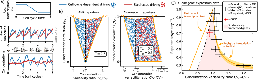
Figure 4: Utilizing bounds to analyze concentrations in growing and dividing cells. A) We want to distinguish stochastically varying transcription rates whose average remains constant throughout the cell-cycle (red line) from transcription rates that change periodically during the cell-cycle (exemplified by blue line). Numbers of molecules oscillate in both types of systems but only systems with cell-cycle dependent driving oscillate in concentrations. Our constraints can identify such periodic gene expression from static snapshots of population variability without access to time-series data. B) Solid orange lines denote open-loop constraints proven for systems in which the reporter concentrations are independent of the cell volume, under the assumption that the cell volume grows exponentially between division events. For mRNA reporters (left panel) concentration correlations are then bounded by the same constraints derived for absolute numbers in the absence of feedback. When transcription rates are periodic, the open-loop constraint of Eq. 2 for absolute numbers does not strictly apply to concentrations. Numerical simulations of example systems (blue dots) suggest that such systems only fall fall marginally outside the orange bounds. For fluorescent reporters (right panel), the feedback bounds (orange lines) for concentrations depend on the additional parameter $T_{m}^{c}:=(1/\tau_{\mathrm{mat},x}+\ln(2)/\tau_{c})/(1/\tau_{\mathrm{mat},y}+\ln(2)/\tau_{c})$ where $\tau_{c}$ is the average cell-cycle time, see Eq. (7). However, for both mRNA and fluorescence levels, Eqs. (4) and (5) (dashed black lines) can be used to detect cell cycle dependent genes from asynchronous static snapshots of dual reporter concentrations. C) Previously reported gene expression variability data for constitutively expressed fluorescent proteins that exhibit first order maturation dynamics in E. coli [15]. Plotted are variability ratios and reporter asymmetries with respect to the observed dynamics of mEYFP. As expected for constitutively expressed fluorescent proteins, the experimental data is consistent with the class of gene expression models that do not exhibit feedback and are not periodically driven (pink region) bounded by Eq.(5) and Eq.(8). With the exception of the indicated mEGFP outlier, all data fall along the right hand boundary that is only accessible for systems whose fluorescence variability is dominated by a translation, maturation, or machine read-out step. The yellow corridor indicates the estimated uncertainty in reported cell-cycle time $\tau_{c}=(28.5\pm 2)$ min and the reference mEYFP maturation half-life $\tau_{mat,y}\ln(2)=(9.0\pm 0.7)$ min. Variability ratios with respect to all other reference fluorescence proteins confirm the above picture with the exception of the observed mEGFP variability which violates the expected behaviour, see Appendix L.

IV.2 Proportional transcription rates

So far we considered co-regulated genes that have identical (though probabilistic) transcription rates. This is motivated by experimental synthetic reporter systems in which two fluorescent proteins are expressed under two identical copies of a known transcriptional promoter. Additionally, the above results can be extended to co-regulated genes in which the transcription rates are not identical but proportional to each other, i.e., $R_{y}=\alpha R_{x}$ for some $\alpha$. Similar bounds hold for this new class of systems (see Appendix I) but they depend on the proportionality factor $\alpha$ which is potentially unknown. For the class of systems defined in Eq. (1) this issue can be resolved by introducing an additional reporter to determine the constant of proportionality between the transcription rates. If the life-time ratio $T$ is not known a priori, then four reporters would be needed in order to determine all unknowns. Additionally, for synthetic fluorescent protein reporters, the constant of proportionality in transcription can be inferred from absolute numbers of molecules. If measurements only report relative numbers, $\alpha$ can be inferred through additional reporter correlations or sequential single-color experiments in which the same fluorescent protein is expressed under the two different promoters (see Appendix J.2).

IV.3 Systematic undercounting

Experimental data in cell biology might not reflect absolute abundances. For example, mRNA molecules are often counted using fluorescence in situ hybridization (FISH), a method that can lead to a systematic undercounting of the copy number due to probabilistic binding between mRNA molecules and the fluorescent probes. Similarly, sequencing methods rely on probabilistic amplification steps to detect transcripts. However, as long as each type molecule is experimentally detected with the same probability, the above bounds and accessible regions are strictly unaffected by the detection probabilities (Appendix H). This can be intuitively understood because undercounting corresponds to a binomial read-out step which de-correlates measurements just like the already accounted for stochastic reaction steps. While reported averages, variances, and correlations strongly depend on detection probabilities, their accessible region is bounded by the same inequalities described above.

If different reporters have a different probability of being detected we can generalize the above constraints to account for that and infer the missing parameter from pairwise correlations between three reporters (see Appendix J.2).

IV.4 Concentration measurements instead of absolute numbers

Growing and dividing cells exhibit a natural cycle in which, on average, cell-division “eliminates” half the molecules of a cell while also reducing the cell volume by a factor of two. Instead of considering absolute numbers, many experiments thus report concentrations of molecules which (on average) are unaffected by cell-division. In the preceding discussion, the specified reactions describe the birth and death of molecules, but exactly the same constraints of Eqs. (4) and (5) can be used to analyze concentration measures of growing and dividing cells. When using concentrations to determine CVs, violations of Eqs. (4) and (5) can then detect genes whose transcription rate varies periodically during the cell-cycle, see Fig. 4. In this analysis of concentrations we allow for binomial splitting noise, division time fluctuations, and asymmetric divisions, and we assume that cellular volume grows exponentially between divisions (Appendix K).

When reporter concentrations are independent of cell volume, open-loop constraints for concentrations similar to the ones derived for absolute numbers can be analytically proven (Appendix K). For co-regulated mRNA this constraint is exactly identical to Eq. (2), but for fluorescent proteins the equivalent of Eq. (3) changes because concentrations are subject to an additional degradation rate from dilution governed by the average cell-cycle time $\tau_{c}$. In the absence of feedback, CVs in fluorescence concentrations that are volume independent are constrained by

$$\text{max}\left(\frac{T_{m}^{c}\frac{CV_{y^{\prime\prime}}}{CV_{x^{\prime\prime}}}-\frac{CV_{x^{\prime\prime}}}{CV_{y^{\prime\prime}}}}{1-T_{m}^{c}},0\right)\leqslant\rho_{x^{\prime\prime}y^{\prime\prime}}\leqslant\frac{\frac{T_{m}^{c}}{T_{m}}\frac{CV_{y^{\prime\prime}}}{CV_{x^{\prime\prime}}}-\frac{CV_{x^{\prime\prime}}}{CV_{y^{\prime\prime}}}}{\frac{T_{m}^{c}}{T_{m}}-1}$$ (7)

where $T_{m}^{c}=(1/\tau_{mat,x}+\ln(2)/\tau_{c})/(1/\tau_{mat,y}+\ln(2)/\tau_{c})$, and these bounds are indicated by the solid orange lines in Fig. 4B (right panel).

Systems in which the reporter concentrations are not independent of the volume are not bound by the above constraints. However, numerical simulations suggest that CVs in concentrations violate inequalities Eqs. (2), (7) only marginally, see blue dots in Fig. 4B. An exact bound can be derived to strictly constrain this class of systems if we have experimental access to a third reporter (see Appendix K.3).

IV.5 Data from constitutively expressed fluorescent proteins fall within the expected bounds

Ultimate proof that our constraints can be used to identify periodically expressed genes will consist of experimentally observing CVs of cell-cycle dependent promoters that violate Eq. (4) or Eq. (5) in physiologically relevant regimes. However, even in the absence of such direct verification, the applicability of our method can be supported through a self-consistency check, i.e., whether data for fluorescent proteins expressed through a constitutive promoter fall into the expected region of gene expression dynamics that is stochastically driven and not subject to feedback control. Such data exists in E. coli for fluorescent proteins with precisely determined maturation dynamics [15]. Here, we analyze this cell-to-cell variability data for fluorescent reporters that exhibited clear first-order maturation dynamics by determining the CV in protein concentration after subtracting volume variability of growing and dividing cells (Appendix L).

In the absence of simultaneous fluorescence measurements, sequential CV measurements in concentrations are constrained by

$$T_{m}^{c}\leqslant\frac{CV_{x^{\prime\prime}}}{CV_{y^{\prime\prime}}}\leqslant\sqrt{\frac{T_{m}^{c}}{T_{m}}},$$ (8)

which corresponds to the bounds of Eq. (7) when allowing for any value of the correlation coefficient (unobserved for sequential variability measurements). As discussed in the previous section, the no-oscillation constraint of Eq. (5) still applies directly even when we analyze concentrations rather than absolute numbers.

In Fig. 4C we present experimentally determined variability data [15] for fluorescent proteins under control of the constitutive promoter proC in E. coli with mEYFP variability and maturation dynamics as a reference point. As expected for constitutively expressed fluorescent proteins, the data for these biologically “boring” systems is consistent with the class of gene expression models that do not exhibit feedback and are not periodically driven (pink region), bounded by Eq.(5) and Eq.(8). Error bars for $T_{m}^{c}$ in Fig. 4C are taken from [15] with error propagation, and error bars in CVs and their ratios are the standard error of the mean from three independent cell cultures with error propagation respectively. Furthermore, all data (with the exception of mEGFP) follow the right boundary of the allowed region. The observed variability of mEGFP is confirmed as an outlier when using the mEGFP measurements as a reference point for which the observed CV-ratios violate our predicted bounds (see Appendix L). One possible explanation of this outlier would be that mEGFP cells grew more slowly than the experimentally reported 28.5 min cell-division times for all strains.

Data that falls on the right hand boundary is consistent with negligible biological noise upstream of translation or with variability that is dominated by technical measurement noise whose normalized variance decreases with the inverse of the mean population signal (see Appendix L).

IV.6 Measurement noise & technological limitations

Theoretical constraints can be experimentally exploited as long as measurement uncertainties are sufficiently small. When considering the sampling error of cell-to-cell variability, 95% confidence intervals for CVs have been reported to be around 5-10% of the respective CV value [12, 19]. Similarly, experiments have shown high biological reproducibility, e.g., three repeats of identical flow-cytometry experiments exhibited a standard error of the CVs of around 10% [15]. However, a significant limitation remains for current experimental high-throughput methods like flow-cytometry or single-cell sequencing: the measurements techniques themselves introduce significant noise, especially when used with bacteria [25, 26], which means that technical variability can introduce a systematic error in estimates of biological variability. In such cases, one can attempt to deconvolve true biological variability from measurement noise using experimental and analytical techniques, e.g., by using calibration beads [25] or by using noise models [26]. Alternatively, one can opt for methods of lower throughput but greater precision, for example, mRNA measurements by single-molecule FISH (smFISH) are well-suited for validation of our method given its accuracy and high sensitivity [27]. Rapid improvements in high throughput quantification tools such as sequential FISH (seqFISH) will provide exciting opportunities for future applications of our work [28].

V Discussion

While our results are motivated by the analysis of gene expression dynamics, utilizing correlation constraints to characterize the dynamics within complex processes may prove useful in other areas of science in which systems involve many interacting components whose dynamics is difficult or impossible to track completely. Our results show that it is possible to rigorously analyze correlations within classes of incompletely specified physical models without resorting to statistical inference methods. Crucially, our approach does not require time-resolved data, which is often unavailable for complex systems. For example, following individual cells over time is much more challenging, and thus less common, than taking static population snapshots of cellular abundances.

Our correlation constraints provide a framework to detect the presence of feedback strictly from observations of a small subset of components within a much larger cellular process. This could, e.g., be utilized to pinpoint molecular components that are involved in feedback regulation of a gene by observing how our proposed signature of feedback is affected in knock-out experiments. Additionally, our results highlight that using unequal reporters can reveal dynamic properties of regulation even in the absence of temporal data. These constraints are fundamentally due to the dynamics of interactions and are not apparent in previous work that considered asymmetric dual reporters as static random variables [29]. For example, we show that theoretically cell-cycle dependent transcription rates can be detected from static population measurements of asymmetric downstream products of gene expression. Additionally, we explicitly show that our mathematical framework can be utilized even when experimental techniques detect individual molecules only probabilistically or when key parameters are unknown. Finally, we report an experimental “negative control” in which we confirm that the measured variability of constitutively expressed fluorescence proteins falls into the expected region of gene expression variability for genes that are not subject to feedback regulation or periodic driving.

Appendix

Here we detail the mathematical derivations and illustrate some of the results in greater depth. Throughout the appendix we denote the normalized (co)variance as $\eta_{fg}:=\text{Cov}(f,g)/(\langle f\rangle\langle g\rangle)$, where the statistical measures are stationary population averages.

First we go over the mathematical framework in which we model reaction networks in cells. The state of an intracellular biochemical network at a given moment in time is given by the integer numbers $\{x_{i}\}$ of the chemical species $\{X_{i}\}$, which we can write as $\mathbf{x}=(x_{1},\dots,x_{n})$. This system is dynamic, and so this state $\mathbf{x}$ will undergo discreet changes over time as reactions occur. If there are $m$ possible reactions in the system, we can write them as

$$\mathbf{x}\xrightarrow[]{\quad r_{k}(\mathbf{x})\quad}\mathbf{x}+\mathbf{d}_{k}\qquad k=1,\dots,m$$

where the rate $r_{k}(\mathbf{x})$ corresponds to the probability per unit time of the $k$-th reaction occurring, and the step size $\mathbf{d}_{k}=(d_{1k},\dots,d_{nk})$ corresponds to the change in the chemical species numbers $\mathbf{x}$ from the $k$-th reaction (the $d_{ik}$ are positive or negative integers). It then follows that the system probability distribution $P(\mathbf{x},t)$ evolves according to the chemical master equation [30, 31]:

$$\frac{d}{dt}P(\mathbf{x},t)=\sum_{k}\left[r_{k}(\mathbf{x}-\mathbf{d}_{k})P(\mathbf{x}-\mathbf{d}_{k},t)-r_{k}(\mathbf{x})P(\mathbf{x},t)\right].$$

Time evolution equations for the moments $\langle x_{i}^{k}\rangle$ of each component $X_{i}$ follow directly from the chemical master equation [31].

Appendix A Fluctuation balance relations for systems as defined in Eq. (1)

Previous work established general relations that constrain fluctuations of components within incompletely specified reaction networks [18]. In particular, any two components Z₁ and Z₂ in an arbitrarily complex network that reach wide-sense stationarity, must satisfy the following flux balance relations

$$\langle R_{1}^{+}\rangle=\langle R_{2}^{-}\rangle,$$ (9)

as well as the following fluctuation balance relations

$$\text{Cov}(z_{1},R_{2}^{-}-R_{2}^{+})+\text{Cov}(z_{2},R_{1}^{-}-R_{1}^{+})=\sum_{k}d_{1k}d_{2k}\langle r_{k}\rangle,$$ (10)

where $R_{i}^{+}$ and $R_{i}^{-}$ are the net birth and death fluxes of component Z_i, and the summation is over all reactions in the network, with $r_{k}$ the rate of the $k$-th reaction, and $d_{ik}$ the step-size of Z_i of the $k$-th reaction. For the class of systems in Eq. (1), Eqs. (9) and (10) imply

$$\langle R\rangle=\langle x\rangle/\tau_{x}\quad\text{\&}\quad\langle R\rangle=\langle y\rangle/\tau_{y},$$ (11)

and

$$\begin{split}&\eta_{xx}=\frac{1}{\langle x\rangle}+\eta_{xR},\quad\eta_{yy}=\frac{1}{\langle y\rangle}+\eta_{yR},\\ &\eta_{xy}=\frac{1}{1+T}\eta_{xR}+\frac{T}{1+T}\eta_{yR}.\end{split}$$ (12)

These relations must be satisfied by all systems in the class, regardless of the unspecified details. This allows us to set general constraints that hold for the entire class of systems. For example, the above relations lead to

$$\eta_{xy} =\frac{1}{1+T}\left(\eta_{xx}-\frac{1}{\langle x\rangle}\right)+\frac{T}{1+T}\left(\eta_{yy}-\frac{1}{\langle y\rangle}\right)$$

$$\leq\frac{1}{1+T}\eta_{xx}+\frac{T}{1+T}\eta_{yy},$$

where in the 2nd step we used fact that the averages are positive. Dividing this bound by $\sqrt{\eta_{xx}\eta_{yy}}$ leads to $\rho_{xy}(1+T)\leqslant\frac{CV_{x}}{CV_{y}}+T\frac{CV_{y}}{CV_{x}}$, which is the bound indicated by the dashed orange line in Fig. 1B. The inequality becomes an equality when $\frac{1}{\langle x\rangle},\frac{1}{\langle y\rangle}\to 0$, which corresponds to systems where $X$ and $Y$ exhibit no intrinsic stochasticity and follow the upstream signal deterministically.

Appendix B Constraints on open-loop systems for systems as define in Eq. (1)

B.1 Derivation of the open-loop constraint Eq. (2)

We consider a hypothetical ensemble of systems from the class of Eq. (1) that all share the same upstream history $\mathbf{u}[-\infty,t]$. We can then consider the average stochastic dual reporters conditioned on the history of their upstream influences [32, 33], which corresponds to the averages at a moment in time in this hypothetical ensemble

$$\bar{x}(t)=\mathrm{E}\big{[}X_{t}|\mathbf{u}[-\infty,t]\big{]}\quad\text{\&}\quad\bar{y}(t)=\mathrm{E}\big{[}Y_{t}|\mathbf{u}[-\infty,t]\big{]}.$$

These are time-dependent variables that depend on the upstream history $\mathbf{u}[-\infty,t]$. We can take averages $\langle\bar{x}\rangle$ and (co)variances $\eta_{\bar{x}\bar{x}}$ over the distribution of all possible histories.

This conditional system is not stationary because of the synchronised rate $R(t)=R(\mathbf{u}(t))$, and so the time-evolution of the averages will follow the following differential equations [32]

$$\begin{split}\frac{d\Delta\bar{x}}{dt}=\Delta R(t)-\Delta\bar{x}(t)/\tau_{x},\\ \frac{d\Delta\bar{y}}{dt}=\Delta R(t)-\Delta\bar{y}(t)/\tau_{y},\end{split}$$ (13)

where $\Delta\bar{x}=\bar{x}-\langle x\rangle$, $\Delta\bar{y}=\bar{y}-\langle y\rangle$, and $\Delta R(t)=R(t)-\langle R\rangle$. These differential equations correspond to a linear response problem in which $X$ and $Y$ both respond to $R(t)$ on different timescales. To relate the results to the actual ensemble we multiply the left differential equation by $\bar{x}$ and take the expectation over all histories $\mathbf{u}[-\infty,t]$ to get

$$\mathrm{E}\left[\frac{1}{2}\frac{d\Delta\bar{x}^{2}}{dt}\right]=\mathrm{E}\big{[}\Delta\bar{x}R(t)\big{]}-\mathrm{E}\big{[}\Delta\bar{x}^{2}\big{]}/\tau_{x}.$$

Note that $\mathrm{E}\left[\frac{d\Delta\bar{x}^{2}}{dt}\right]=\frac{d}{dt}\mathrm{E}\big{[}\Delta\bar{x}^{2}\big{]}=\frac{d}{dt}\text{Var}(\bar{x})$, which equals zero at wide-sense stationarity. We thus have

$$\text{Cov}(\bar{x},\Delta R(t))=\text{Var}(\bar{x})/\tau_{x}.$$

Moreover, we have

$$\text{Cov}(\bar{x},R(t))=\mathrm{E}\big{[}\bar{x}R(t)\big{]}-\mathrm{E}\big{[}\bar{x}\big{]}\cdot\mathrm{E}\big{[}R(t)\big{]}$$

$$=\mathrm{E}\big{[}\mathrm{E}[X_{t}|\mathbf{u}[-\infty,t]]\cdot R(t)\big{]}-\langle x\rangle\langle R\rangle$$

$$=\mathrm{E}\big{[}\mathrm{E}[X_{t}R(\mathbf{u}(t))|\mathbf{u}[-\infty,t]]\big{]}-\langle x\rangle\langle R\rangle$$

$$=\langle xR\rangle-\langle x\rangle\langle R\rangle=\text{Cov}(X,R).$$

Putting these results together and normalizing we find

$$\eta_{\bar{x}\bar{x}}=\eta_{xR}\quad\text{\&}\quad\eta_{\bar{y}\bar{y}}=\eta_{yR},$$ (14)

where the flux-balance relations Eq. (11) were used and the expression on the right follows by symmetry. Similarly, it has been shown [32] that $\eta_{\bar{x}\bar{y}}=\eta_{xy}$. Comparing with the fluctuation-balance relations Eq. (12), we find

$$\begin{split}&\eta_{xx}=\frac{1}{\langle x\rangle}+\eta_{\bar{x}\bar{x}},\quad\eta_{yy}=\frac{1}{\langle y\rangle}+\eta_{\bar{y}\bar{y}},\\ &\eta_{\bar{x}\bar{y}}=\eta_{xy}=\frac{1}{1+T}\eta_{\bar{x}\bar{x}}+\frac{T}{1+T}\eta_{\bar{y}\bar{y}}.\end{split}$$ (15)

These relations allow us to translate results derived from the deterministic dynamics to the stochastic dynamics. We now use Cauchy-Schwarz as follows

$$\left(\frac{1}{1+T}\eta_{\bar{x}\bar{x}}+\frac{T}{1+T}\eta_{\bar{y}\bar{y}}\right)^{2}=\eta_{\bar{x}\bar{y}}^{2}\leq\eta_{\bar{x}\bar{x}}\eta_{\bar{y}\bar{y}}.$$

This inequality leads to a quadratic that can be solved to obtained the following inequality

$$T^{2}\eta_{\bar{y}\bar{y}}\leq\eta_{\bar{x}\bar{x}}\leq\eta_{\bar{y}\bar{y}}.$$ (16)

We need to write this inequality in terms of the measurable (co)variances $\eta_{xx}$, $\eta_{yy}$, and $\eta_{xy}$. To do this, note that the flux-balance equations Eq. (11) and the fluctuation-balance equations Eq. (12) comprise a linear system of 5 equations and 5 unknowns. We can thus solve for $\eta_{xR}$ and $\eta_{yR}$ in terms of the measurable (co)variances

$$\begin{split}\eta_{xR}=\frac{(1+T)\eta_{xy}-T\eta_{yy}+\eta_{xx}}{2},\\ \eta_{yR}=\frac{(1+T)\eta_{xy}+T\eta_{yy}-\eta_{xx}}{2T}.\end{split}$$ (17)

From Eq. (14) we find that $\eta_{\bar{x}\bar{x}}=\eta_{xR}$ and $\eta_{\bar{y}\bar{y}}=\eta_{yR}$, so we substitute Eq. (17) into Eq. (16), which leads to the open-loop constraint of Eq. (2).

B.2 Discriminating types of feedback

The open-loop constraint of Eq. (2) constrains all systems from the class of Eq. (1) in which $X$ and $Y$ are not connected in some kind of feedback loop. Here we derive similar constraints on systems where only one of the components undergoes open-loop regulation, while the other can still be connected in a feedback loop. We will also show how co-regulated reporters can be used to infer whether or not the feedback is negative, and if so, how to measure the noise suppression from this negative feedback using only (co)variance measurements.

First, we consider systems in which there is no feedback in one of the components, say $X$. We can then condition on the history of the upstream variables $\mathbf{u}(t)$ and the history of $Y$ — together they make a larger cloud of components that can affect $X$ but are not affected by $X$. Just like the previous section, we then consider the conditional average $\bar{x}=\mathrm{E}[X_{t}|\mathbf{u}[-\infty,t],y[-\infty,t]]$, from which we have

$$\mathrm{E}[\bar{x}(t)y(t)]-\mathrm{E}[\bar{x}]\mathrm{E}[y(t)]=\dots$$

$$=\mathrm{E}\Big{[}\mathrm{E}\big{[}X_{t}y(t)|\mathbf{u}[-\infty,t],y[-\infty,t]\big{]}\Big{]}-\langle x\rangle\langle y\rangle$$

$$=\mathrm{E}\Big{[}\mathrm{E}\big{[}X_{t}Y_{t}|\mathbf{u}[-\infty,t],y[-\infty,t]\big{]}\Big{]}-\langle x\rangle\langle y\rangle$$

$$=\langle xy\rangle-\langle x\rangle\langle y\rangle\Rightarrow\eta_{\bar{x}y}=\eta_{xy}\quad.$$

We can then use the Cauchy-Schwarz inequality in the following way: $\eta_{xy}^{2}=\eta_{\bar{x}y}^{2}\leq\eta_{\bar{x}\bar{x}}\eta_{yy}$. This inequality bounds systems in which there is no feedback in $X$. We would now like to write it in terms of measurable (co)variances. To do this, we note that the relation $\eta_{\bar{x}\bar{x}}=\eta_{xR}$ from Eq. (14) still holds here as we made no assumptions about $Y$ in that derivation. We can thus use Eq. (17) to write $\eta_{\bar{x}\bar{x}}$ in terms of the measurable (co)variances and subsitute the results in the above inequality. This leads to the following constraint

$$\rho_{xy}^{2}\leq\frac{1}{2}\left((1+T)\rho_{xy}\frac{CV_{y}}{CV_{x}}-T\left(\frac{CV_{y}}{CV_{x}}\right)^{2}+1\right).$$ (18)

Systems that break this constraint must have some kind of feedback in $X$. Similarly, we can derive the analogous constraint on systems with no feedback in $Y$:

$$\rho_{xy}^{2}\leq\frac{1}{2T}\left((1+T)\rho_{xy}\frac{CV_{x}}{CV_{y}}+T-\left(\frac{CV_{x}}{CV_{y}}\right)^{2}\right).$$ (19)

Systems that break this constraint must have some kind of feedback in $Y$. These bounds are plotted in Fig. 5A.

Next, we show how to detect negative feedback. Here we define feedback to be negative when $\eta_{xR}<0$. That is, the birthrate $R$ acts to suppress noise in $X$ below poisson noise. From Eq. (17), $\eta_{xR}$ and $\eta_{yR}$ can be solved for in terms of the measurable (co)variances. (Co)variance measurements between co-regulated mRNA can thus be used to measure $\eta_{xR}$ and $\eta_{yR}$ using Eq. (17), see Fig. 5B. Moreover, we can quantify how strong this negative feedback is through the noise suppression : $\eta_{xx}/(1/\langle x\rangle)=\eta_{xx}/(\eta_{xx}-\eta_{xR})$. As the negative feedback gets stronger, the noise suppression will get smaller and quantifies the strength of the negative feedback.

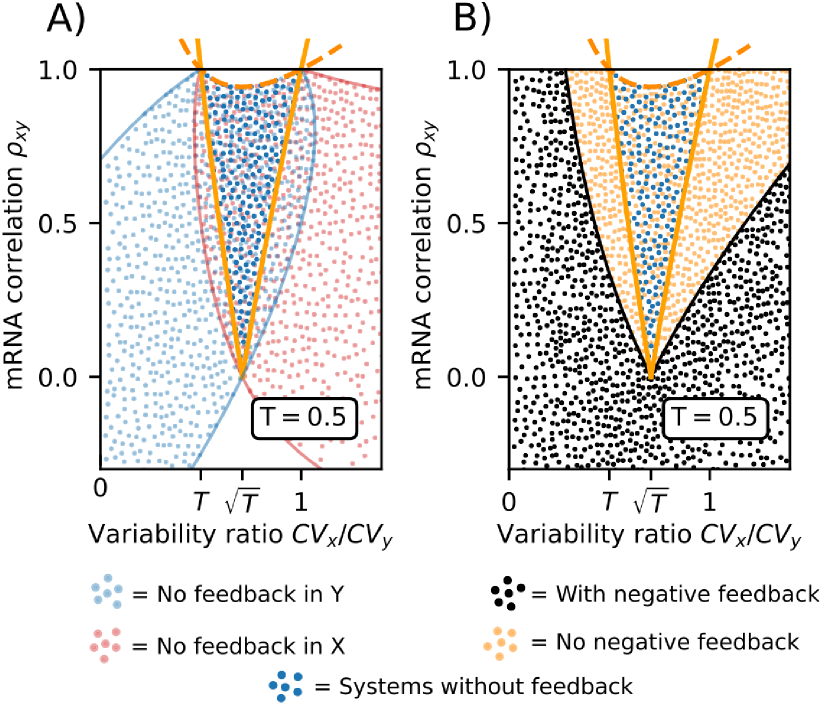
Figure 5: The space of possible covariability between mRNA-levels of co-regulated genes depends on the type of feedback A) Systems that have no feedback in $X$ must lie in the region bounded by the light-red solid lines which corresponds to the region bounded by Eq. (18). Systems that lie outside of this region must have feedback in X. Similarly, systems that have no feedback in $Y$ must lie in the region bounded by the light-blue solid lines which corresponds to the region bounded by Eq. (19). B) Here we define feedback to be negative when the mRNA transcription rate is negatively correlated with the mRNA levels: $\eta_{xR}<0$. This would correspond to highly regulated systems that exhibit noise suppression. Using co-regulated reporters, $\eta_{xR}$ and $\eta_{yR}$ can be measured from static (co)variance measurements of $X$ and $Y$ using Eq. (17).

Appendix C Dynamics from static transcript variability

The stationary solution for the variance of $\bar{x}(t)$ follows from the linear response problem Eq. (13) with

$$\eta_{\bar{x}\bar{x}}=\frac{1}{\tau_{x}}\eta_{RR}\int_{0}^{\infty}A(s)e^{-s/\tau_{x}}\mathrm{d}s,$$ (20)

where $A(s)$ is the auto-correlation of the time-varying transcription rate $R(t)$ (see below for a detailed derivation). For a given input $R(t)$, $\eta_{\bar{x}\bar{x}}$ depends on $\tau_{x}$, and so measuring $\tau_{x}\eta_{\bar{x}\bar{x}}$ as a function of $\tau_{x}$ effectively determines the Laplace Transform of the auto-correlation of $R(t)$ from static variance measurements of downstream reporters. Our results exploit the fact that knowing static downstream variability for just two values of $\tau_{x}$ constrains the possible dynamics of $R(t)$.

In particular, with $\tau_{y}<\tau_{x}$ we have

$$\eta_{\bar{x}\bar{x}}-T\eta_{\bar{y}\bar{y}}=\frac{\eta_{RR}}{\tau_{x}}\int_{0}^{\infty}A(s)\left(e^{-s/\tau_{x}}-e^{-s/\tau_{y}}\right)\mathrm{d}s.$$ (21)

For stochastic upstream signals with $A(s)\geq 0$ the integrand of Eq. (21) is non-negative such that

$$T\eta_{\bar{y}\bar{y}}\leq\eta_{\bar{x}\bar{x}}.$$ (22)

Eq. (22) gives the bound of Eq. (4) after substituting $\eta_{\bar{x}\bar{x}}=\eta_{xx}-1/\langle x\rangle$ and $\eta_{\bar{y}\bar{y}}=\eta_{yy}-1/\langle y\rangle$ together with the flux balance given by Eq. (11).

We can further bound the class of stochastic systems based on the timescale of the upstream fluctuations. If upstream fluctuations are slower than $\tau_{R}$ such that $A(s)\geq e^{-s/\tau_{R}}$, we have

$$\eta_{\bar{x}\bar{x}}-T\eta_{\bar{y}\bar{y}} \geq\frac{\eta_{RR}}{\tau_{x}}\int_{0}^{\infty}e^{-t/\tau_{R}}\left(e^{-t/\tau_{x}}-e^{-t/\tau_{y}}\right)\mathrm{d}t$$

$$=\eta_{RR}\tau_{R}\left(\frac{1}{\tau_{R}+\tau_{x}}-\frac{T}{\tau_{R}+\tau_{y}}\right)$$

$$\geq\eta_{\bar{y}\bar{y}}\tau_{R}\left(\frac{1}{\tau_{R}+\tau_{x}}-\frac{T}{\tau_{R}+\tau_{y}}\right),$$

and analogously to the above derivation of Eq. (4), it follows that

$$\beta(1-T)\rho_{xy}\leqslant\dfrac{CV_{x}}{CV_{y}}-T\dfrac{CV_{y}}{CV_{x}},$$ (23)

where $\beta=(1+T)/\left(2T(1+\frac{\tau_{x}}{\tau_{R}})(1+T\frac{\tau_{x}}{\tau_{R}})+(1-T)\right)$. In the limit where $\tau_{R}\to 0$ we have $\beta\to 0$, and as a result Eq. (23) converges to Eq. (4). Conversely, for slow stochastic upstream fluctuations as $\tau_{R}\to\infty$ we have $\beta\to 1$, and Eq. (23) converges to the right boundary of the open-loop constraint (see Fig. 6). The analytical bound of Eq. (23) is marginally loose. A tight bound can be derived numerically as presented in the Supplemental Material [34].

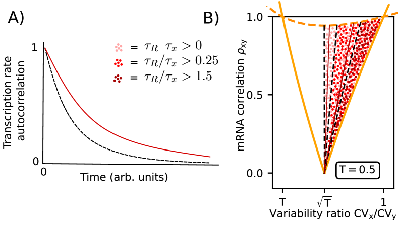
Figure 6: The space of possible correlations between co-regulated reporters depends on the timescale of the upstream fluctuations. A) The timescale of stochastic fluctuations is characterized by how quickly the auto-correlation of the signal (red) decays to zero. By bounding the auto-correlation from below by $e^{-t/\tau_{R}}$ (black dashed curve) we set a lower bound on how quickly the signal auto-correlation can decay to zero. This thus sets a lower bound on the ”speed” of the signal fluctuations. B) Open-loop systems in which the upstream auto-correlation is bounded below by $e^{-t/\tau_{R}}$ are bounded further towards the right. The solid dark red lines correspond to the loose bound given by Eq. (23), whereas the black dashed lines are given by the stricter nuerical bound presented in the supplement [34]. These constraints can be used to gain information on the timescale of upstream fluctuations with only access to static snapshots of dual reporter transcript concentrations obtained, e.g., from single-cell sequencing methods that report snapshots of transcript abundances rather than temporal information.

Derivation of Eq. (20): Taking the Fourier transforms of Eq. (13) and using the Wiener-Khinchin theorem [35] which states that the spectral density of a random signal is equal to the Fourier transform of its autocorrelation, we find

$$\mathcal{F}[\mathcal{R}_{\bar{x}}]=\frac{\mathcal{F}[\mathcal{R}_{R}]}{(1+\omega^{2})}\quad\text{\&}\quad\mathcal{F}[\mathcal{R}_{\bar{y}}]=\frac{\mathcal{F}[\mathcal{R}_{R}]/T^{2}}{(1/T^{2}+\omega^{2})},$$

where $\mathcal{R}_{R}$ is the autocovariance of $R$. Since $\mathcal{R}_{R}(t=0)=\text{Var}(R)$, the variances can be found by taking the inverse Fourier transforms at $t=0$

$$\begin{split}&\text{Var}(\bar{x})=\frac{1}{2\pi}\int_{-\infty}^{\infty}\frac{\mathcal{F}[\mathcal{R}_{R}]}{(1+\omega^{2})}d\omega,\\ &\text{Var}(\bar{y})=\frac{1}{2\pi}\int_{-\infty}^{\infty}\frac{\mathcal{F}[\mathcal{R}_{R}]}{(1/T^{2}+\omega^{2})}d\omega.\end{split}$$ (24)

We thus have

$$\begin{split}&\text{Var}(\bar{y})=\dots\\ &=\frac{1}{2\pi}\int_{-\infty}^{\infty}\mathcal{F}[\mathcal{R}_{R}](\omega)\left(\frac{T^{2}}{1+(\omega T)^{2}}\right)d\omega\\ &=\frac{1}{2\pi}\int_{-\infty}^{\infty}\left[\int_{-\infty}^{\infty}\mathcal{R}_{R}(t)e^{-i\omega t}dt\right]\left(\frac{T^{2}}{1+(\omega T)^{2}}\right)d\omega\\ &=\frac{1}{2\pi}\int_{-\infty}^{\infty}\left[\int_{-\infty}^{\infty}\mathcal{R}_{R}(t)\text{cos}(\omega t)dt\right]\left(\frac{T^{2}}{1+(\omega T)^{2}}\right)d\omega\\ &=\frac{1}{2\pi}\int_{-\infty}^{\infty}\int_{-\infty}^{\infty}\mathcal{R}_{R}(t)\text{cos}(\omega t)\left(\frac{T^{2}}{1+(\omega T)^{2}}\right)dtd\omega\\ &=\frac{1}{2\pi}\int_{-\infty}^{\infty}\mathcal{R}_{R}(t)\left[\int_{-\infty}^{\infty}\text{cos}(\omega t)\left(\frac{T^{2}}{1+(\omega T)^{2}}\right)d\omega\right]dt\\ &=\frac{1}{2}\int_{-\infty}^{\infty}\mathcal{R}_{R}(t)Te^{-|t|/T}dt\\ &=\int_{0}^{\infty}\mathcal{R}_{R}(t)Te^{-t/T}dt,\end{split}$$

where in the third step we use the fact that $\mathcal{R}_{R}(t)$ is real and symmetric, and in the last step we use the fact that the integrand is symmetric in $t$. Normalizing by the averages, we have Eq. (20). Note that this expression can also be derived by writing down the general solution of $\Delta\bar{y}(t)$ from the differential equation Eq. (13), squaring the solution to get $\Delta\bar{y}(t)^{2}$, and taking the ensemble average over all histories, where ergodicity is not assumed.

Setting bounds on the spectral density of upstream influences using co-regulated reporters

Numerical simulations of sinusoidal driving indicate that slow oscillations lie along the right hand side of the open-loop region in Fig. 1B, and move towards the left as the frequency of oscillation increases. Here we derive approximate conditions for how large an oscillation frequency needs to be to break the constraint given by Eq. (4) of the main text. In particular, systems in which the spectral density of the upstream signal $|\mathcal{F}[R]|^{2}(\omega)$ is zero for all $\omega\geq\omega_{u}$ are bounded by the following inequality

$$\begin{split}\left(T\frac{CV_{y}}{CV_{x}}-\frac{CV_{x}}{CV_{y}}\right)\frac{(1+T)}{(\gamma+T)}\geq(T-\gamma)\rho_{xy}\\ \text{where}\quad\gamma=\left(\frac{1+\omega_{u}^{2}\tau_{y}^{2}}{1+\omega_{u}^{2}\tau_{x}^{2}}\right).\end{split}$$ (25)

Systems that break the above inequality cannot satisfy the requirement that $|\mathcal{F}[R]|^{2}(\omega)=0$ for all $\omega\geq\omega_{u}$. Similarly, systems in which the spectral density of the upstream signal $|\mathcal{F}[R]|^{2}(\omega)$ is zero for all $\omega\leq\omega_{u}$ are bounded by the following inequality

$$\begin{split}(T-\gamma)\rho_{xy}\leq\left(T\frac{CV_{y}}{CV_{x}}-\frac{CV_{x}}{CV_{y}}\right)\frac{(1+T)}{(\gamma+T)}\\ \text{where}\quad\gamma=\left(\frac{1+\omega_{u}^{2}\tau_{y}^{2}}{1+\omega_{u}^{2}\tau_{x}^{2}}\right).\end{split}$$ (26)

Systems that break the above inequality cannot satisfy the requirement that $|\mathcal{F}[R]|^{2}(\omega)=0$ for all $\omega\leq\omega_{u}$.

Eqs. (25) and (26) bound fast oscillations towards the left and slow oscillations towards the right of the open-loop region in Fig. 1B. As an oscillatory signal will have a peak in its spectral density centered at the angular frequency of the oscillation, Eqs. (25) and (26) provide us with an estimation for how fast an upstream oscillation needs to be relative to the reporter lifetimes in order for the system to cross the no-oscillation line and be fully discriminated from stochastic signals. In particular, setting $\gamma=T$ turns (26) into the ”no-oscillation constraint” given by Eq. (4) of the main text, and turns Eq. (25) into the opposite constraint which constrains systems to be in the region only accessible by oscillations. This $\gamma=T$ is achieved when $\omega_{u}=1/\sqrt{\tau_{x}\tau_{y}}$. We thus have the following approximate requirement for how fast the upstream signal needs to oscillate relative to the reporter lifetimes in order to break the no-oscillation bound

$$\frac{1}{\sqrt{\tau_{x}\tau_{y}}}\lesssim\omega_{R}=2\pi f_{R},$$ (27)

where $f_{R}$ is the frequency of the upstream oscillation.

We will now derive the bounds that were just presented. We normalize Eq. (24) by the averages

$$\begin{split}&\eta_{\bar{x}\bar{x}}=\frac{1}{2\pi\langle x\rangle^{2}}\int_{-\infty}^{\infty}\frac{|\mathcal{F}[R]|^{2}}{1+\omega^{2}}d\omega\\ &\eta_{\bar{y}\bar{y}}=\frac{1}{2\pi\langle x\rangle^{2}}\int_{-\infty}^{\infty}\frac{|\mathcal{F}[R]|^{2}}{1+\omega^{2}T^{2}}d\omega,\end{split}$$ (28)

where without loss of generality we work in units where $\tau_{x}=1$ and $\tau_{y}=T$, and where we use the fact that $\langle y\rangle=T\langle x\rangle$. We thus have

$$\eta_{\bar{x}\bar{x}}-\left(\frac{1+\omega_{u}^{2}T^{2}}{1+\omega_{u}^{2}}\right)\eta_{\bar{y}\bar{y}}=\frac{1}{2\pi\langle x\rangle^{2}}\int_{-\infty}^{\infty}|\mathcal{F}[R]|^{2}\left(\frac{1}{1+\omega^{2}}-\left(\frac{1+\omega_{u}^{2}T^{2}}{1+\omega_{u}^{2}}\right)\frac{1}{1+\omega^{2}T^{2}}\right)d\omega.$$

The expression in square brackets is negative for $\omega>\omega_{u}$ and positive otherwise. Thus, if the spectral density of $R$ is zero for $\omega\geq\omega_{u}$, we have

$$\eta_{\bar{x}\bar{x}}-\left(\frac{1+\omega_{u}^{2}T^{2}}{1+\omega_{u}^{2}}\right)\eta_{\bar{y}\bar{y}}\geq 0.$$

Using Eq. (14) and Eq. (17) to write $\eta_{\bar{x}\bar{x}}$ and $\eta_{\bar{y}\bar{y}}$ in terms of measurable (co)variances, this inequality becomes Eq. (25). Similarly, the same arguments show that systems in which the spectral density of $R$ is zero for all $\omega\leq\omega_{u}$ must satisfy Eq. (26).

Appendix D The general class of co-regulated fluorescent proteins

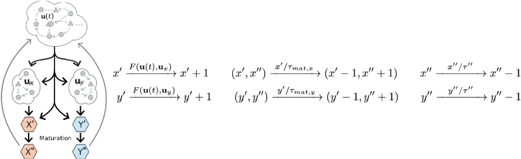
Figure 7: General class of dual reporter systems with co-regulated fluorescent proteins We consider a class of systems identical to Fig. 2A with the exception that we now include multiple unspecified steps in the intrinsic dynamics of gene expression. Here $\mathbf{u}_{x}$ and $\mathbf{u}_{y}$ are identical (though independent) systems of components that are affected by the upstream cloud of components $\mathbf{u}(t)$ in the same way. These two smaller clouds of components model the intrinsic steps in gene expression and allow for a wide range of possible mRNA dynamics and post-translational modifications that occur before the maturation step. They are left unspecified except for the fact that we assume they do not form circuits of components that can create oscillations, so that any oscillatory variability is caused by the shared environment $\mathbf{u}(t)$. We model the dynamics of immature fluorescent proteins denoted as X’ and Y’, as well as mature fluorescent proteins X” and Y”. The birthrate of X’ and Y’ can now depend on the components in $\mathbf{u}_{x}$ and $\mathbf{u}_{y}$ respectively, in an arbitrary way. The asymmetry between the co-regulated genes is characterized by the ratio of average fluorescent maturation times $T_{\mathrm{m}}:=\tau_{\mathrm{mat},y}/\tau_{\mathrm{mat},x}$.

For the class of fluorescent proteins defined in Fig. 2A we can derive similar results. First, however, we will define a more general class of systems from which Fig. 2A is a subset. This class consists of the class of systems in Fig. 2A when we don’t make any assumptions about the mRNA intrinsic system, see Fig. 7. Here, $\mathbf{u}_{x}$ and $\mathbf{u}_{y}$ are systems of variables that model the mRNA dynamics after transcription or any post-translational modifications that occur before the maturation step. Together with $\mathbf{u}(t)$ these form a larger “cloud” of components that affect the proteins $X^{\prime}$ and $Y^{\prime}$. We require that $\mathbf{u}_{x}$ and $\mathbf{u}_{y}$ are identical, though independent (in the sense that they are not equal, as the shared influence of $\mathbf{u}(t)$ will make them statistically dependent). Aside from this they are left almost completely unspecified. We will make one additional requirement on these non-specified intrinsic systems when we prove the open-loop constraint given by Eq. (3) of the main text. In particular, we require that the fluctuations that originate from these intrinsic systems be non-oscillatory, so that any oscillatory variability is caused by variability in the shared upstream environment $\mathbf{u}(t)$. Specifically, the birthrates of X’ and Y’ will not be entirely equal due to random fluctuations that originate from the intrinsic systems. This intrinsic noise can be quantified as the difference between the two translation rates: $F(\mathbf{u}(t),\mathbf{u}_{x})-F(\mathbf{u}(t),\mathbf{u}_{y})$. This difference is a stochastic signal, and here we require that the autocorrelation of this signal be non-negative. This assumption holds for the class in Fig. 2A and in systems where the intrinsic systems consist of an otherwise unspecified cascade of arbitrary steps. The assumption excludes systems in which $\mathbf{u}_{x}$ and $\mathbf{u}_{y}$ form circuits of components that create oscillations.

Similarly to Appendix A, at wide-sense stationarity the following flux-balance relations must hold [18]

$$\begin{split}&\langle x^{\prime\prime}\rangle/\tau^{\prime\prime}=\langle x^{\prime}\rangle/\tau_{max,x}=\langle F_{x}\rangle,\quad\\ &\langle y^{\prime\prime}\rangle/\tau^{\prime\prime}=\langle y^{\prime}\rangle/\tau_{max,y}=\langle F_{y}\rangle,\end{split}$$ (29)

where $F_{x}:=F(\mathbf{u}(t),\mathbf{u}_{x})$ and $F_{y}:=F(\mathbf{u}(t),\mathbf{u}_{y})$. In addition, the following fluctuation-balance relations must hold,

$$\begin{split}\eta_{x^{\prime}x^{\prime}}=\frac{1}{\langle x^{\prime}\rangle}+\eta_{x^{\prime}F_{x}},\quad\eta_{y^{\prime}y^{\prime}}=\frac{1}{\langle y^{\prime}\rangle}+\eta_{y^{\prime}F_{y}},\quad\eta_{x^{\prime}y^{\prime}}=\frac{1}{1+T_{m}}\eta_{x^{\prime}F_{y}}+\frac{T_{m}}{1+T_{m}}\eta_{y^{\prime}F_{x}},\\ \eta_{x^{\prime\prime}x^{\prime\prime}}=\frac{1}{\langle x^{\prime\prime}\rangle}+\eta_{x^{\prime}x^{\prime\prime}},\quad\eta_{y^{\prime\prime}y^{\prime\prime}}=\frac{1}{\langle y^{\prime\prime}\rangle}+\eta_{y^{\prime}y^{\prime\prime}},\quad\eta_{x^{\prime\prime}y^{\prime\prime}}=\frac{1}{2}\eta_{y^{\prime}x^{\prime\prime}}+\frac{1}{2}\eta_{x^{\prime}y^{\prime\prime}},\\ \eta_{x^{\prime}x^{\prime\prime}}=\frac{1}{1+\frac{\tau^{\prime\prime}}{\tau_{mat,x}}}\eta_{x^{\prime}F_{x}}+\frac{\frac{\tau^{\prime\prime}}{\tau_{mat,x}}}{1+\frac{\tau^{\prime\prime}}{\tau_{mat,x}}}\eta_{x^{\prime\prime}F_{x}},\quad\eta_{y^{\prime}y^{\prime\prime}}=\frac{1}{1+\frac{\tau^{\prime\prime}}{\tau_{mat,y}}}\eta_{y^{\prime}F_{y}}+\frac{\frac{\tau^{\prime\prime}}{\tau_{mat,y}}}{1+\frac{\tau^{\prime\prime}}{\tau_{mat,y}}}\eta_{y^{\prime\prime}F_{y}},\\ \eta_{y^{\prime}x^{\prime\prime}}=\frac{1}{1+\frac{\tau^{\prime\prime}}{\tau_{mat,y}}}\eta_{x^{\prime}y^{\prime}}+\frac{\frac{\tau^{\prime\prime}}{\tau_{mat,y}}}{1+\frac{\tau^{\prime\prime}}{\tau_{mat,y}}}\eta_{x^{\prime\prime}F_{y}},\quad\eta_{x^{\prime}y^{\prime\prime}}=\frac{1}{1+\frac{\tau^{\prime\prime}}{\tau_{mat,x}}}\eta_{x^{\prime}y^{\prime}}+\frac{\frac{\tau^{\prime\prime}}{\tau_{mat,x}}}{1+\frac{\tau^{\prime\prime}}{\tau_{mat,x}}}\eta_{y^{\prime\prime}F_{x}}.\end{split}$$ (30)

Appendix E Constraints on open-loop systems for systems as define in Fig. 2A

Here we prove the inequality Eq. (3). The inequality Eq. (3) has three parts, which are represented by the three solid orange lines in Fig. 2B in the paper. We will first prove these three constraints one at a time, followed by the upper bound on correlations illustrated by the dashed orange line in Fig. 2B. Refer back to Fig. 7 for illustration of the system being studied.

Proof of the bottom bound $\rho_{x^{\prime\prime}y^{\prime\prime}}\geq 0$: Just like in the previous sections, we consider the average stochastic dual reporter dynamics conditioned on the history of their upstream influences

$$\bar{x}^{\prime\prime}(t)=\mathrm{E}\big{[}X^{\prime\prime}_{t}|\mathbf{u}[-\infty,t]\big{]}\quad\text{\&}\quad\bar{y}^{\prime\prime}(t)=\mathrm{E}\big{[}Y^{\prime\prime}_{t}|\mathbf{u}[-\infty,t]\big{]}.$$

When the cloud of components $\mathbf{u}(t)$ is not affected by the downstream components we can write the time evolution of the conditional averages using the chemical master equation of the conditional probability space

$$\frac{d\Delta\bar{x}^{\prime}}{dt}=\Delta\bar{F}(t)-\Delta\bar{x}^{\prime}\qquad\frac{d\Delta\bar{y}^{\prime}}{dt}=\Delta\bar{F}(t)-\Delta\bar{y}^{\prime}/T_{m}\quad$$

$$\frac{d\Delta\bar{x}^{\prime\prime}}{dt}=\Delta\bar{x}^{\prime}-\Delta\bar{x}^{\prime\prime}/\tau^{\prime\prime}\qquad\frac{d\Delta\bar{y}^{\prime\prime}}{dt}=\Delta\bar{y}^{\prime}/T_{m}-\Delta\bar{y}^{\prime\prime}/\tau^{\prime\prime}$$

where without loss of generality we work in units where $\tau_{mat,x}=1$ and $\tau_{mat,y}=T_{m}$, and where

$$\bar{F}(t) =\mathrm{E}\big{[}F(\mathbf{u}(t),\mathbf{u}_{x})|\mathbf{u}[-\infty,t]\big{]}$$

$$=\mathrm{E}\big{[}F(\mathbf{u}(t),\mathbf{u}_{y})|\mathbf{u}[-\infty,t]\big{]},$$

is the translation rate after averaging out the mRNA fluctuations. Note that the equality on the right hand side is from the fact that the unspecified intrinsic systems $\mathbf{u}_{x}$ and $\mathbf{u}_{y}$ are identical and thus the conditional averages are the same. Taking the Fourier transform of the above differential equations, and then using the Wiener-Khinchin theorem [35] which states that the spectral density of a random signal is equal to the Fourier transform of its autocorrelation, we find

$$\mathcal{F}[\mathcal{R}_{\bar{x}}]=\frac{\mathcal{F}[\mathcal{R}_{\bar{F}}]}{(1/\tau^{\prime\prime 2}+\omega^{2})(1+\omega^{2})},$$

$$\mathcal{F}[\mathcal{R}_{\bar{y}}]=\frac{\mathcal{F}[\mathcal{R}_{\bar{F}}]}{(1/\tau^{\prime\prime 2}+\omega^{2})(1+\omega^{2}T_{m}^{2})},$$

where $\mathcal{R}_{\bar{F}}$ is the autocovariance of $\bar{F}(t)$. Since $\mathcal{R}_{z}(t=0)=\text{Var}(z)$, the variances can be found by taking the inverse Fourier transforms at $t=0$

$$\begin{split}&\text{Var}(\bar{x}^{\prime\prime})=\frac{1}{2\pi}\int_{-\infty}^{\infty}\frac{\mathcal{F}[\mathcal{R}_{\bar{F}}]}{(1/\tau^{\prime\prime 2}+\omega^{2})(1+\omega^{2})}d\omega\\ &\text{Var}(\bar{y}^{\prime\prime})=\frac{1}{2\pi}\int_{-\infty}^{\infty}\frac{\mathcal{F}[\mathcal{R}_{\bar{F}}]}{(1/\tau^{\prime\prime 2}+\omega^{2})(1+\omega^{2}T_{m}^{2})}d\omega.\end{split}$$ (31)

Moreover, we then use the Wiener-Khinchin theorem [35] which states that the Fourier transform of the cross power spectral density of two signals is equal to the Fourier transform of their cross-correlation to write

$$\mathcal{F}[\mathcal{R}_{\bar{x}^{\prime\prime},\bar{y}^{\prime\prime}}]=\frac{\mathcal{F}[\mathcal{R}_{\bar{F}}](1/T_{m}+\omega^{2}+i\omega(1-1/T_{m}))/T_{m}}{(1/\tau^{\prime\prime 2}+\omega^{2})(1+\omega^{2})(1/T_{m}^{2}+\omega^{2})},$$

where $\mathcal{R}_{\bar{x}^{\prime\prime},\bar{y}^{\prime\prime}}$ is the cross-covariance of $\bar{x}^{\prime\prime}(t)$ and $\bar{y}^{\prime\prime}(t)$. Taking the inverse Fourier transform at $t=0$ gives us the covariance

$$\text{Cov}(\bar{x}^{\prime\prime},\bar{y}^{\prime\prime})=$$

$$\frac{1}{2\pi}\int_{-\infty}^{\infty}\mathcal{F}[\mathcal{R}_{\bar{F}}]\frac{(1/T_{m}+\omega^{2})/T_{m}}{(1/\tau^{\prime 2}+\omega^{2})(1+\omega^{2})(1/T_{m}^{2}+\omega^{2})}d\omega,$$

where the term proportional to $i\omega$ integrated to zero because it was odd in $\omega$ whereas the rest of the integrand is even in $\omega$ through $\mathcal{F}[\mathcal{R}_{\bar{F}}]=|\mathcal{F}[\Delta\bar{F}]|^{2}$. We thus have

$$(1+T_{m})\text{Cov}(\bar{x}^{\prime\prime},\bar{y}^{\prime\prime})=$$

$$= \frac{1}{2\pi}\int_{-\infty}^{\infty}\mathcal{F}[\mathcal{R}_{\bar{F}}]\frac{(1+T_{m})(1/T_{m}+\omega^{2})/T_{m}}{(1/\tau^{\prime 2}+\omega^{2})(1+\omega^{2})(1/T_{m}^{2}+\omega^{2})}d\omega$$

$$= \frac{1}{2\pi}\int_{-\infty}^{\infty}\mathcal{F}[\mathcal{R}_{\bar{F}}]\frac{1}{(1+\omega^{2})(1/\tau^{\prime 2}+\omega^{2})}d\omega$$

$$\quad+\frac{T_{m}}{2\pi}\int_{-\infty}^{\infty}\mathcal{F}[\mathcal{R}_{\bar{F}}]\frac{1}{(1+\omega^{2}T_{m}^{2})(1/\tau^{\prime 2}+\omega^{2})}d\omega$$

$$= \text{Var}(\bar{x}^{\prime\prime})+T_{m}\text{Var}(\bar{y}^{\prime\prime}).$$

Upon normalizing with the averages we have

$$\eta_{\bar{x}^{\prime\prime}\bar{y}^{\prime\prime}}=\frac{1}{1+T_{m}}\eta_{\bar{x}^{\prime\prime}\bar{x}^{\prime\prime}}+\frac{T_{m}}{1+T_{m}}\eta_{\bar{y}^{\prime\prime}\bar{y}^{\prime\prime}}.$$

Moreover,

Cov $$(\bar{x}^{\prime\prime},\bar{y}^{\prime\prime})=\dots$$

$$=\mathrm{E}\big{[}\mathrm{E}[X^{\prime\prime}_{t}|\mathbf{u}[-\infty,t]]\cdot\mathrm{E}[Y^{\prime\prime}_{t}|\mathbf{u}[-\infty,t]]\big{]}$$

$$\qquad-\mathrm{E}\big{[}\mathrm{E}[X^{\prime\prime}_{t}|\mathbf{u}[-\infty,t]]\big{]}\cdot\mathrm{E}\big{[}\mathrm{E}[Y^{\prime\prime}_{t}|\mathbf{u}[-\infty,t]]\big{]}$$

$$=\mathrm{E}\big{[}\mathrm{E}[X^{\prime\prime}_{t}Y^{\prime\prime}_{t}|\mathbf{u}[-\infty,t]]\big{]}-\langle x^{\prime\prime}\rangle\langle y^{\prime\prime}\rangle$$

$$=\langle x^{\prime\prime}y^{\prime\prime}\rangle-\langle x^{\prime\prime}\rangle\langle y^{\prime\prime}\rangle=\text{Cov}(x^{\prime\prime},y^{\prime\prime}),$$

where the 3rd step comes from the fact that $X^{\prime\prime}$ and $Y^{\prime\prime}$ are independent when we condition on the upstream history $\mathbf{u}[-\infty,t]$ [33]. Upon normalizing by the averages we have $\eta_{\bar{x}^{\prime\prime}\bar{y}^{\prime\prime}}=\eta_{x^{\prime\prime}y^{\prime\prime}}$, and so

$$\eta_{x^{\prime\prime}y^{\prime\prime}}=\frac{1}{1+T_{m}}\eta_{\bar{x}^{\prime\prime}\bar{x}^{\prime\prime}}+\frac{T_{m}}{1+T_{m}}\eta_{\bar{y}^{\prime\prime}\bar{y}^{\prime\prime}}\geq 0.$$ (32)

We thus have the lower bound $\rho_{x^{\prime\prime}y^{\prime\prime}}\geq 0$ .

Proof of the right bound $CV_{x^{\prime\prime}}/CV_{y^{\prime\prime}}\leq 1$ : Here we will need to consider the average stochastic dual reporter dynamics conditioned on the history of all their upstream influences

$$\bar{\bar{x}}^{\prime\prime}(t):=\mathrm{E}\big{[}X^{\prime\prime}_{t}|\mathbf{u}[-\infty,t],\mathbf{u}_{x}[-\infty,t]\big{]}\quad$$

$$\bar{\bar{y}}^{\prime\prime}(t):=\mathrm{E}\big{[}Y^{\prime\prime}_{t}|\mathbf{u}[-\infty,t],\mathbf{u}_{y}[-\infty,t]\big{]},$$

where now we also condition on the trajectory of the mRNA dynamics. When the cloud of components $\mathbf{u}(t)$ does not depend on the downstream components we can write down the time evolution of the conditional averages using the chemical master equation of the conditional probability space. The time evolution of the conditional averages $\bar{\bar{y}}^{\prime}$ and $\bar{\bar{y}}^{\prime\prime}$ is given by

$$\frac{d\bar{\bar{y}}^{\prime}}{dt}=F_{y}(t)-\bar{\bar{y}}^{\prime}/T_{m}\quad\text{\&}\quad\frac{d\bar{\bar{y}}^{\prime\prime}}{dt}=\bar{\bar{y}}^{\prime}/T_{m}-\bar{\bar{y}}^{\prime\prime}/\tau^{\prime\prime},$$

where now $F_{y}(t)$ corresponds to a particular translation rate trajectory as we no longer average out the mRNA dynamics, and without loss of generality we let $\tau_{mat,x}=1$ and $\tau_{mat,y}=T_{m}$. In terms of the deviations from the means these differential equations become

$$\begin{split}\frac{d\Delta\bar{\bar{y}}^{\prime}}{dt}&=\Delta F_{y}(t)-\Delta\bar{\bar{y}}^{\prime}/T_{m},\\ \frac{d\Delta\bar{\bar{y}}^{\prime\prime}}{dt}&=\Delta\bar{\bar{y}}^{\prime}/T_{m}-\Delta\bar{\bar{y}}^{\prime\prime}/\tau^{\prime\prime},\end{split}$$ (33)

Multiplying the left and right equations with $\Delta\bar{\bar{y}}^{\prime\prime}$ and $\Delta\bar{\bar{y}}^{\prime}$ respectively, summing the results, and taking ensemble averages of the different upstream histories gives us

$$\mathrm{E}\left[\frac{d}{dt}(\Delta\bar{\bar{y}}^{\prime}\bar{\bar{y}}^{\prime\prime})\right]=$$

$$\mathrm{E}\big{[}\Delta\bar{\bar{y}}^{\prime\prime}\Delta F_{y}\big{]}+\mathrm{E}\big{[}\Delta\bar{\bar{y}}^{\prime 2}\big{]}/T_{m}-\left(\frac{1}{T_{m}}+\frac{1}{\tau^{\prime\prime}}\right)\mathrm{E}\big{[}\Delta\bar{\bar{y}}^{\prime}\Delta\bar{\bar{y}}^{\prime\prime}\big{]}.$$

At stationarity the left hand side is zero, so we have

$$\left(\frac{1}{T_{m}}+\frac{1}{\tau^{\prime\prime}}\right)\mathrm{E}\big{[}\Delta\bar{\bar{y}}^{\prime}\Delta\bar{\bar{y}}^{\prime\prime}\big{]}=\mathrm{E}\big{[}\Delta\bar{\bar{y}}^{\prime\prime}\Delta F_{y}\big{]}+\mathbf{E}\big{[}(\bar{\bar{y}}^{\prime})\big{]}/T_{m}.$$

Similarly, multiplying the first equation in Eq. (33) by $\Delta\bar{\bar{y}}^{\prime}$, taking the ensemble average, and using the fact that the left hand side will be zero at stationarity, we have

$$\mathrm{E}\big{[}\Delta\bar{\bar{y}}^{\prime}\Delta\bar{\bar{y}}^{\prime}\big{]}=T_{m}\mathrm{E}\big{[}\Delta\bar{\bar{y}}^{\prime}\Delta F_{y}\big{]}.$$

Now mutiplying the second equation in Eq. (33) by $\Delta\bar{\bar{y}}^{\prime\prime}$ and following the same steps we have

$$\mathrm{E}\big{[}\bar{\bar{y}}^{\prime\prime}\bar{\bar{y}}^{\prime\prime}\big{]}/\tau^{\prime\prime}=T_{m}\mathrm{E}\big{[}\bar{\bar{y}}^{\prime}\bar{\bar{y}}^{\prime\prime}\big{]}.$$

Combining these expressions gives us

$$\left(\frac{1}{T_{m}}+\frac{1}{\tau^{\prime\prime}}\right)\text{Var}(\bar{\bar{y}}^{\prime\prime})=\text{Cov}(\bar{\bar{y}}^{\prime\prime},F_{y})+\text{Cov}(\bar{\bar{y}}^{\prime},F_{y}).$$

Now note that

$$\text{Cov}(\bar{\bar{y}}^{\prime\prime},F_{y})=\mathrm{E}\big{[}\bar{\bar{y}}^{\prime\prime}\cdot F_{y}(t)\big{]}-\mathrm{E}\big{[}\bar{\bar{y}}^{\prime\prime}\big{]}\cdot\mathrm{E}\big{[}F_{y}\big{]}$$

$$=\mathrm{E}\big{[}\mathrm{E}[Y^{\prime\prime}_{t}|\mathrm{u}[-\infty,t],\mathbf{u}_{y}[-\infty,t]]\cdot F_{y}(t)\big{]}-\mathrm{E}\big{[}\mathrm{E}[Y_{t}|\mathrm{u}[-\infty,t],\mathbf{u}_{y}[-\infty,t]]\big{]}\cdot\mathrm{E}\big{[}\mathrm{E}[F(\mathbf{u}(t),\mathbf{u}_{y}(t)|\mathrm{u}[-\infty,t],\mathbf{u}_{y}[-\infty,t]]\big{]}$$

$$=\mathrm{E}\big{[}\mathrm{E}[Y^{\prime\prime}_{t}\cdot F_{y}(\mathbf{u}(t),\mathbf{u}_{y}(t))|\mathrm{u}[-\infty,t],\mathbf{u}_{y}[-\infty,t]]\big{]}-\langle y^{\prime\prime}\rangle\langle F_{y}\rangle=\text{Cov}(y^{\prime\prime},F_{y}),$$

and similarly $\text{Cov}(\bar{\bar{y}}^{\prime},F_{y})=\text{Cov}(y^{\prime},F_{y})$. Thus, after normalizing with the averages, we have

$$\eta_{\bar{\bar{y}}^{\prime}\bar{\bar{y}}^{\prime}}=\frac{1}{1+\frac{\tau^{\prime\prime}}{T_{m}}}\eta_{y^{\prime}F_{y}}+\frac{\frac{\tau^{\prime\prime}}{T_{m}}}{1+\frac{\tau^{\prime\prime}}{T_{m}}}\eta_{y^{\prime\prime}F_{y}}.$$

This is the expression for $\eta_{y^{\prime}y^{\prime\prime}}$ in the fluctuation-balance equations Eq. (30), and so

$$\eta_{\bar{\bar{x}}^{\prime\prime}\bar{\bar{x}}^{\prime\prime}}=\eta_{x^{\prime\prime}x^{\prime\prime}}-1/\langle x^{\prime\prime}\rangle\quad\text{\&}\quad\eta_{\bar{\bar{y}}^{\prime\prime}\bar{\bar{y}}^{\prime\prime}}=\eta_{y^{\prime\prime}y^{\prime\prime}}-1/\langle y^{\prime\prime}\rangle,$$ (34)

where the $x^{\prime\prime}$ expression follows by symmetry. Moreover, we apply the same analysis that was done in the previous proof to write

$$\begin{split}&\text{Var}(\bar{\bar{x}}^{\prime\prime})=\frac{1}{2\pi}\int_{-\infty}^{\infty}\frac{\mathcal{F}[\mathcal{R}_{F_{x}}]}{(1/\tau^{\prime\prime 2}+\omega^{2})(1+\omega^{2})}d\omega,\\ &\text{Var}(\bar{\bar{y}}^{\prime\prime})=\frac{1}{2\pi}\int_{-\infty}^{\infty}\frac{\mathcal{F}[\mathcal{R}_{F_{y}}]}{(1/\tau^{\prime\prime 2}+\omega^{2})(1+\omega^{2}T_{m}^{2})}d\omega,\end{split}$$ (35)

where $\mathcal{R}_{F_{x}}$ and $\mathcal{R}_{F_{y}}$ are the autocovariances of the translation rates $F(\mathbf{u}(t),\mathbf{u}_{x})$ and $F(\mathbf{u}(t),\mathbf{u}_{y})$. Note that since the two intrinsic systems $\mathbf{u}_{x}$ and $\mathbf{u}_{y}$ are statistically identical, we have $\mathcal{R}_{F_{x}}=\mathcal{R}_{F_{y}}$, and so the $\text{Var}(\bar{\bar{y}}^{\prime\prime})$ expression has a larger integrande for all $\omega$ (recall that $\mathcal{F}[\mathcal{R}_{F_{y}}]=\mathcal{F}[\Delta F_{y}]^{2}$ and so is positive). We thus have $\text{Var}(\bar{\bar{x}}^{\prime\prime})<\text{Var}(\bar{\bar{y}}^{\prime\prime})$, which after normalizing gives us $\eta_{\bar{\bar{x}}^{\prime\prime}\bar{\bar{x}}^{\prime\prime}}\leq\eta_{\bar{\bar{y}}^{\prime\prime}\bar{\bar{y}}^{\prime\prime}}$. From Eq. (29) we have $\langle x^{\prime\prime}\rangle=\langle y^{\prime\prime}\rangle$, and so by using Eq. (34) we find the right bound $CV_{x^{\prime\prime}x^{\prime\prime}}\leq CV_{y^{\prime\prime}y^{\prime\prime}}$.

Proof of the left bound: Recall from the previous two proofs we derived the following equations

$$\begin{split}\eta_{x^{\prime\prime}x^{\prime\prime}}=\frac{1}{\langle x^{\prime\prime}\rangle}+\eta_{\bar{\bar{x}}^{\prime\prime}\bar{\bar{x}}^{\prime\prime}}\quad\quad\eta_{y^{\prime\prime}y^{\prime\prime}}=\frac{1}{\langle y^{\prime\prime}\rangle}+\eta_{\bar{\bar{y}}^{\prime\prime}\bar{\bar{y}}^{\prime\prime}}\\ \eta_{x^{\prime\prime}y^{\prime\prime}}=\eta_{\bar{x}^{\prime\prime}\bar{y}^{\prime\prime}}=\frac{1}{1+T_{m}}\eta_{\bar{x}^{\prime\prime}\bar{x}^{\prime\prime}}+\frac{T_{m}}{1+T_{m}}\eta_{\bar{y}^{\prime\prime}\bar{y}^{\prime\prime}}.\end{split}$$ (36)

We now use the Cauchy-Schwarz inequality with the last expression

$$\left(\frac{1}{1+T_{m}}\eta_{\bar{x}^{\prime\prime}\bar{x}^{\prime\prime}}+\frac{T_{m}}{1+T_{m}}\eta_{\bar{y}^{\prime\prime}\bar{y}^{\prime\prime}}\right)^{2}\leq\eta_{\bar{x}^{\prime\prime}\bar{x}^{\prime\prime}}\eta_{\bar{y}^{\prime\prime}\bar{y}^{\prime\prime}},$$

which leads to

$$T_{m}^{2}\eta_{\bar{y}^{\prime\prime}\bar{y}^{\prime\prime}}\leq\eta_{\bar{x}^{\prime\prime}\bar{x}^{\prime\prime}}\leq\eta_{\bar{y}^{\prime\prime}\bar{y}^{\prime\prime}}.$$ (37)

Unlike the mRNA system of equations, we cannot solve Eq. (36) for $\eta_{\bar{x}^{\prime\prime}\bar{x}^{\prime\prime}}$ and $\eta_{\bar{y}^{\prime\prime}\bar{y}^{\prime\prime}}$ in terms of the measurable (co)variances because the system is underdetermined. This is due to the fact that we have not specified the mRNA intrinsic system. Nevertheless, we can derive an additional bound that will allow us to close the system of equations to write Eq. (37) in terms of the measurable (co)variances.

From Eqs. (31) and  (35) we have

$$\text{Var}(\bar{\bar{x}}^{\prime\prime})-\text{Var}(\bar{x}^{\prime\prime}) =\frac{1}{2\pi}\int_{-\infty}^{\infty}\frac{\mathcal{F}[\mathcal{R}_{F_{x}}-\mathcal{R}_{\bar{F}}]}{(1/\tau^{\prime\prime 2}+\omega^{2})(1+\omega^{2})}d\omega.$$

Now, note that

$$\mathcal{R}_{\bar{F}}(t) =\mathrm{E}\big{[}\mathrm{E}[\Delta F(\mathbf{u}(t^{\prime}),\mathbf{u}_{x})|\mathbf{u}[-\infty,t^{\prime}]]\cdot\mathrm{E}[\Delta F(\mathbf{u}(t^{\prime}+t),\mathbf{u}_{x})|\mathbf{u}[-\infty,t^{\prime}+t]]\big{]}$$

$$=\mathrm{E}\big{[}\mathrm{E}[\Delta F(\mathbf{u}(t^{\prime}),\mathbf{u}_{x})|\mathbf{u}[-\infty,t^{\prime}]]\cdot\mathrm{E}[\Delta F(\mathbf{u}(t^{\prime}+t),\mathbf{u}_{y})|\mathbf{u}[-\infty,t^{\prime}+t]]\big{]}$$

$$=\mathrm{E}\big{[}\mathrm{E}[\Delta F(\mathbf{u}(t^{\prime}),\mathbf{u}_{x})\cdot\Delta F(\mathbf{u}(t^{\prime}+t),\mathbf{u}_{y})|\mathbf{u}[-\infty,t^{\prime}+t]]\big{]}=\text{Cov}(F_{x}(t^{\prime}),F_{y}(t^{\prime}+t))=\mathcal{R}_{F_{x},F_{y}}(t),$$

where the second step comes from the fact that $F_{x}$ and $F_{y}$ are statistically equivalent and the third step comes from the fact that they are independent when we condition on the upstream history $\mathbf{u}[-\infty,t]$. Taking the autocovariance of $F_{x}-F_{y}$ gives us

$$\mathcal{R}_{F_{x}-F_{y}}=2\mathcal{R}_{F_{x}}-2\mathcal{R}_{F_{x},F_{y}}=2(\mathcal{R}_{F_{x}}-\mathcal{R}_{\bar{F}}).$$

Thus the requirement that we make for this class of systems — that the autocorrelation of $F_{x}-F_{y}$ be non-negative — is equivalent to saying that $\mathcal{R}_{F_{x}}-\mathcal{R}_{\bar{F}}$ is non-negative. Thus, we have

$$\text{Var}(\bar{\bar{x}}^{\prime\prime})-\text{Var}(\bar{x}^{\prime\prime})=\frac{1}{2\pi}\int_{-\infty}^{\infty}\frac{\mathcal{F}[\mathcal{R}_{F_{x}}-\mathcal{R}_{\bar{F}}]}{(\frac{1}{\tau^{\prime\prime 2}}+\omega^{2})(1+\omega^{2})}d\omega$$

$$\text{Var}(\bar{\bar{y}}^{\prime\prime})-\text{Var}(\bar{y}^{\prime\prime})=\frac{1}{2\pi}\int_{-\infty}^{\infty}\frac{\mathcal{F}[\mathcal{R}_{F_{y}}-\mathcal{R}_{\bar{F}}]}{(\frac{1}{\tau^{\prime\prime 2}}+\omega^{2})(1+T_{m}^{2}\omega^{2})}d\omega.$$

Since the two intrinsic systems $\mathbf{u}_{x}$ and $\mathbf{u}_{y}$ are identical, we have $\mathcal{R}_{F_{x}}=\mathcal{R}_{F_{y}}$. Defining $f:=\mathcal{R}_{F_{x}}-\mathcal{R}_{\bar{F}}$, we have

$$(\text{Var}(\bar{\bar{x}})-\text{Var}(\bar{x}))-T_{m}(\text{Var}(\bar{\bar{y}})-\text{Var}(\bar{y}))=\dots$$

$$=\frac{1}{2\pi}\int_{-\infty}^{\infty}\mathcal{F}[f]\left\{\frac{1}{(1+\omega^{2})(1/\tau^{\prime\prime 2}+\omega^{2})}-\frac{T_{m}}{(1+(\omega T_{m})^{2})(1/\tau^{\prime\prime 2}+\omega^{2})}\right\}d\omega$$

$$=\frac{1}{2\pi}\int_{-\infty}^{\infty}\int_{-\infty}^{\infty}f(t)\text{cos}(\omega t)\left\{\frac{1}{(1/\tau^{\prime\prime 2}+\omega^{2})(1+\omega^{2})}-\frac{T_{m}}{(1/\tau^{\prime\prime 2}+\omega^{2})(1+(\omega T_{m})^{2})}\right\}dtd\omega$$

$$=\frac{1}{2\pi}\int_{-\infty}^{\infty}f(t)\left(\int_{-\infty}^{\infty}\frac{\text{cos}(\omega t)}{(1/\tau^{\prime\prime 2}+\omega^{2})}\left\{\frac{1}{(1+\omega^{2})}-\frac{T_{m}}{1+(\omega T_{m})^{2}}\right\}d\omega\right)dt$$

$$=\frac{1}{\pi}\int_{0}^{\infty}f(t)\left(\int_{-\infty}^{\infty}\frac{\text{cos}(\omega t)}{(1/\tau^{\prime\prime 2}+\omega^{2})}\left\{\frac{1}{(1+\omega^{2})}-\frac{T_{m}}{1+(\omega T_{m})^{2}}\right\}d\omega\right)dt$$

$$=\int_{0}^{\infty}f(t)\tau^{\prime\prime 2}\left(\frac{(e^{-t}-\tau^{\prime\prime}e^{-t/\tau^{\prime\prime}})}{(1-\tau^{\prime\prime 2})}-\frac{(T_{m}e^{-t/T_{m}}-\tau^{\prime\prime}e^{-t/\tau^{\prime\prime}})}{(T_{m}^{2}-\tau^{\prime\prime 2})}\right)dt,$$

where in the second step we used the fact that $f(t)$ is symmetric which lets us omit the $\text{sin}(\omega t)$ part of the Fourier transform, and in the fourth step we use the fact that the integrand is symmetric in $t$. The expression in parentheses is always positive, and since $f(t)$ is non-negative, this means that $T_{m}\left(\text{Var}(\bar{\bar{y}})-\text{Var}(\bar{y})\right)\leq\left(\text{Var}(\bar{\bar{x}})-\text{Var}(\bar{x})\right)$, which in terms of the normalized variances is $T_{m}(\eta_{\bar{\bar{y}}^{\prime\prime}\bar{\bar{y}}^{\prime\prime}}-\eta_{\bar{y}^{\prime\prime}\bar{y}^{\prime\prime}})\leq(\eta_{\bar{\bar{x}}^{\prime\prime}\bar{\bar{x}}^{\prime\prime}}-\eta_{\bar{x}^{\prime\prime}\bar{x}^{\prime\prime}})$. Similarly, we can show using the same method that $(\eta_{\bar{\bar{x}}^{\prime\prime}\bar{\bar{x}}^{\prime\prime}}-\eta_{\bar{x}^{\prime\prime}\bar{x}^{\prime\prime}})\leq(\eta_{\bar{\bar{y}}^{\prime\prime}\bar{\bar{y}}^{\prime\prime}}-\eta_{\bar{y}^{\prime\prime}\bar{y}^{\prime\prime}})$. Combining these two inequalities, we have

$$T_{m}\leq\frac{\eta_{\bar{\bar{x}}^{\prime\prime}\bar{\bar{x}}^{\prime\prime}}-\eta_{\bar{x}^{\prime\prime}\bar{x}^{\prime\prime}}}{\eta_{\bar{\bar{y}}^{\prime\prime}\bar{\bar{y}}^{\prime\prime}}-\eta_{\bar{y}^{\prime\prime}\bar{y}^{\prime\prime}}}\leq 1.$$ (38)

With this inequality we can “close” the system of equations Eq. (36) to set the limits of $\eta_{\bar{x}^{\prime\prime}\bar{x}^{\prime\prime}}$ and $\eta_{\bar{y}^{\prime\prime}\bar{y}^{\prime\prime}}$ in terms of the measurable (co)variances

$$\begin{split}\frac{\eta_{x^{\prime\prime}y^{\prime\prime}}(1+T_{m})-T_{m}\left(\eta_{y^{\prime\prime}y^{\prime\prime}}-\eta_{x^{\prime\prime}x^{\prime\prime}}\right)}{1+T_{m}}\leq&\eta_{\bar{x}^{\prime\prime}\bar{x}^{\prime\prime}}\leq\frac{(1+T_{m})\eta_{x^{\prime\prime}y^{\prime\prime}}+\eta_{x^{\prime\prime}x^{\prime\prime}}-T_{m}\eta_{y^{\prime\prime}y^{\prime\prime}}}{2}\\ \frac{\eta_{x^{\prime\prime}y^{\prime\prime}}(1+T_{m})-\eta_{x^{\prime\prime}x^{\prime\prime}}+T_{m}\eta_{y^{\prime\prime}y^{\prime\prime}}}{2T_{m}}\leq&\eta_{\bar{y}^{\prime\prime}\bar{y}^{\prime\prime}}\leq\frac{\eta_{x^{\prime\prime}y^{\prime\prime}}\left(1+T_{m}\right)-\eta_{x^{\prime\prime}x^{\prime\prime}}+\eta_{y^{\prime\prime}y^{\prime\prime}}}{1+T_{m}}.\end{split}$$ (39)

We can then substitute these in the open-loop constraint Eq. (37) to obtain the open-loop constraint in terms of the measurable (co)variances. Doing so we obtain the left bound of Fig. 2B.

Proof of the upper correlation bound: We use the law of total variance to write

$$\eta_{x^{\prime\prime}x^{\prime\prime}}=\eta_{int,x^{\prime\prime}}+\eta_{\bar{x}^{\prime\prime}\bar{x}^{\prime\prime}}\quad\text{\&}\quad\eta_{y^{\prime\prime}y^{\prime\prime}}=\eta_{int,y^{\prime\prime}}+\eta_{\bar{y}^{\prime\prime}\bar{y}^{\prime\prime}}$$

where $\eta_{int,x^{\prime\prime}}=\frac{1}{\langle x^{\prime\prime}\rangle^{2}}\mathrm{E}\big{[}\mathrm{Var}\left(X^{\prime\prime}|\mathbf{u}[-\infty,t]\right)\big{]}$ and $\eta_{int,y^{\prime\prime}}=\frac{1}{\langle y^{\prime\prime}\rangle^{2}}\mathrm{E}\big{[}\mathrm{Var}\left(Y^{\prime\prime}|\mathbf{u}[-\infty,t]\right)\big{]}$. Thus we have $\eta_{x^{\prime\prime}x^{\prime\prime}}\geq\eta_{\bar{x}^{\prime\prime}\bar{x}^{\prime\prime}}$ and $\eta_{y^{\prime\prime}y^{\prime\prime}}\geq\eta_{\bar{y}^{\prime\prime}\bar{y}^{\prime\prime}}$. Substituting in Eq. (32) gives

$$\eta_{x^{\prime\prime}y^{\prime\prime}}(1+T_{m})\leq\eta_{x^{\prime\prime}x^{\prime\prime}}+T_{m}\eta_{y^{\prime\prime}y^{\prime\prime}},$$

which after dividing by $\sqrt{\eta_{x^{\prime\prime}x^{\prime\prime}}\eta_{y^{\prime\prime}y^{\prime\prime}}}$ results in the upper correlation bound.

Appendix F Dynamics from static fluorescent protein variability

When there is no feedback, we can write down the time-evolution equations for the averages of the conditional probability space, and from these we can derive Eq. (35)

$$\text{Var}(\bar{\bar{x}}^{\prime\prime})=\frac{1}{2\pi}\int_{-\infty}^{\infty}\frac{\mathcal{F}[\mathcal{R}_{F_{x}}]}{(1/\tau^{\prime\prime 2}+\omega^{2})(1+\omega^{2})}d\omega,$$

$$\text{Var}(\bar{\bar{y}}^{\prime\prime})=\frac{1}{2\pi}\int_{-\infty}^{\infty}\frac{\mathcal{F}[\mathcal{R}_{F_{y}}]}{(1/\tau^{\prime\prime 2}+\omega^{2})(1+\omega^{2}T_{m}^{2})}d\omega.$$

We then have

$$\text{Var}(\bar{\bar{y}}^{\prime\prime}) =\frac{1}{2\pi}\int_{-\infty}^{\infty}\frac{\mathcal{F}[\mathcal{R}_{F_{y}}]}{(1/\tau^{\prime\prime 2}+\omega^{2})(1+\omega^{2}T_{m}^{2})}d\omega$$

$$=\frac{1}{2\pi}\int_{-\infty}^{\infty}\left[\int_{-\infty}^{\infty}\mathcal{R}_{F_{y}}(t)\text{cos}(\omega t)dt\right]\left(\frac{1}{(1/\tau^{\prime\prime 2}+\omega^{2})(1+(\omega T_{m})^{2})}\right)d\omega$$

$$=\frac{1}{2\pi}\int_{-\infty}^{\infty}\mathcal{R}_{F_{y}}(t)\left(\int_{-\infty}^{\infty}\frac{\text{cos}(\omega t)}{(1/\tau^{\prime\prime 2}+\omega^{2})}\left(\frac{1}{1+(\omega T_{m})^{2}}\right)d\omega\right)dt$$

$$=\frac{1}{\pi}\int_{0}^{\infty}\mathcal{R}_{F_{y}}(t)\left(\int_{-\infty}^{\infty}\frac{\text{cos}(\omega t)}{(1/\tau^{\prime\prime 2}+\omega^{2})}\left(\frac{1}{1+(\omega T_{m})^{2}}\right)d\omega\right)dt$$

$$=\int_{0}^{\infty}\mathcal{R}_{F_{y}}(t)\tau^{\prime\prime 2}\left(\frac{T_{m}e^{-t/T_{m}}-\tau^{\prime\prime}e^{-t/\tau^{\prime\prime}}}{T_{m}^{2}-\tau^{\prime\prime 2}}\right)dt,$$

where the second step comes from the fact that $\mathcal{R}_{F_{y}}(t)$ is and symmetric so we can omit the $\text{sin}(\omega t)$ part of the Fourier transform, and the 4th step comes from the fact that the integrand is symmetric in $t$. We thus have, after normalizing with the averages,

$$\eta_{\bar{\bar{x}}^{\prime\prime}\bar{\bar{x}}^{\prime\prime}}=\int_{0}^{\infty}\eta_{FF}A_{F_{x}}(t)\left(\frac{\tau_{mat,x}e^{-\frac{t}{\tau_{mat,x}}}-\tau^{\prime\prime}e^{-\frac{t}{\tau^{\prime\prime}}}}{\tau_{mat,x}^{2}-\tau^{\prime\prime 2}}\right)dt,$$

$$\eta_{\bar{\bar{y}}^{\prime\prime}\bar{\bar{y}}^{\prime\prime}}=\int_{0}^{\infty}\eta_{FF}A_{F_{y}}(t)\left(\frac{\tau_{mat,y}e^{-\frac{t}{\tau_{mat,y}}}-\tau^{\prime\prime}e^{-\frac{t}{\tau^{\prime\prime}}}}{\tau_{mat,y}^{2}-\tau^{\prime\prime 2}}\right)dt.$$

where $A_{F_{x}}(t)=A_{F_{y}}(t)$ is the autocorrelation of the translation rate $F(\mathbf{u}(t),\mathbf{u}_{x})$. When $A_{F_{x}}\geq 0$, we find that the integrands of the above integrals are always non-negative. Upon comparing them we find that

$$T_{m}\eta_{\bar{\bar{y}}^{\prime\prime}\bar{\bar{y}}^{\prime\prime}}\leq\eta_{\bar{\bar{x}}^{\prime\prime}\bar{\bar{x}}^{\prime\prime}}.$$

Using Eq. (34), and the fact that $\langle x^{\prime\prime}\rangle=\langle y^{\prime\prime}\rangle$ from Eq. (29), the above inequality becomes $T_{m}\eta_{y^{\prime\prime}y^{\prime\prime}}\leq\eta_{x^{\prime\prime}x^{\prime\prime}}$, which in terms of the CVs becomes Eq. (5) of the main text. Note, that the exact same analysis can be used to derive

$$T_{m}\eta_{\bar{y}^{\prime\prime}\bar{y}^{\prime\prime}}\leq\eta_{\bar{x}^{\prime\prime}\bar{x}^{\prime\prime}},$$ (40)

which constrains the reporter (co)variances when the autocorrelation of $\bar{F}(t)=\mathrm{E}\big{[}F(\mathbf{u}(t),\mathbf{u}_{x})|\mathbf{u}[-\infty,t]\big{]}$ is stochastic. Note that $\bar{F}(t)$ is the translation rate when we average out all the mRNA intrinsic fluctuations. This latter constraint will be used in the section on stronger constraints on fluorescent reporters using a third reporter.

Appendix G Behaviour of specific example systems

To gain an intuition for where systems fall in the allowable region we present several example systems in the main text. For example, the arrowed curves in Fig. 1B correspond to two toy models subject to an upstream component Z that undergoes Poisson fluctuations

$$\vspace{-.5em}z\xrightarrow{\mathmakebox{\lambda}}z+1\quad \quad z\xrightarrow{\mathmakebox{z/\tau_{z}}}z-1.\vspace{-.5em}$$

The blue curve in Fig. 1B corresponds to the system $R(\mathbf{u}(t))=kz$, with $k=10$, $\tau_{x}=1$, $\tau_{y}=T$, $\langle z\rangle=\tau_{z}\lambda=100$. As we increase the speed of the upstream fluctuations by decreasing $\tau_{z}$, the dual reporter correlations move downwards and left towards the bound of Eq. (4). This makes intuitive sense because in that regime X and Y have little time to adjust to changing Z levels and de-correlate.

In contrast, the grey curve in Fig. 1B corresponds to a system with feedback of Y onto its own production, with $R(\mathbf{u}(t))=kz/(1+\epsilon y)$, with $k=10$, $\tau_{x}=1$, $\tau_{y}=T$, $\tau_{z}=1$, and $\langle z\rangle=100$. For $\epsilon=0$, we have no feedback and the grey line coincides with the previous system (blue curve) with $\langle x\rangle=\langle y\rangle/T=1000$. As we increase the strength of the feedback $\epsilon$, the correlations of this example system moves outside the region constrained by Eq. (2) when $\epsilon>0,0.07,0.01$ for $T=1,0.5,0.1$ respectively. Maximizing the discriminatory power of the approach corresponds to minimizing the area in which systems without feedback could lie. Choosing $T=1$ or $T\ll 1$ would thus be ideal to detect feedback in this system.

In Fig. 3C the red curve corresponds to a system stochastically driven through a Poisson variable Z with $\tau_{z}=1$, $\langle z\rangle=100$ and $R(\mathbf{u}(t))=kz$ with $k=10$ so that $\langle x\rangle=1000$. In contrast, the blue curve corresponds to a system driven by an oscillation with $R(\mathbf{u}(t))=K(\sin(\omega t+\phi)+2)$, where $\phi$ is a random variable that de-synchronizes the ensemble and $K=500$ so that $\langle x\rangle=1000$. We set the oscillation period $2\pi/\omega=2\tau_{x}$ to model an oscillation set by the cell-cycle (for example, the maturation time of mEGFP is roughly half of the E. coli cell-cycle [15]). We analyzed both types of systems for fixed $\tau_{x}=1$ while varying $\tau_{y}=T$ to see which choice of $T$ maximizes the discriminatory power of the constraint. We find that for this particular example, the oscillating system crossed the dashed black curve when $\omega=1/\sqrt{\tau_{x}\tau_{y}}$.

Appendix H The effects of stochastic undercounting on dual reporter correlations

H.1 Undercounting mRNA

First we analyze the effects of undercounting on mRNA-levels of co-regulated genes. We would like to know how the derived bounds change when the reporter abundances $X$ and $Y$ are detected with fixed probabilities $p_{x}$ and $p_{y}$ respectively. This is done by introducing two new variables that correspond to the experimental readouts of the reporter abundances: $X_{r}$ and $Y_{r}$. In particular, $X_{r}$ corresponds to the detected number of $X$ molecules when each molecule is detected with probability $p_{x}$ (and similarly for $Y_{r}$ and $p_{y}$). In terms of these variables, open-loop systems are constrained by the following inequalities

$$\begin{split}-&\left(\eta_{x_{r}x_{r}}-\frac{p_{y}}{p_{x}}T\eta_{y_{r}y_{r}}\right)\leq\eta_{x_{r}y_{r}}\left(\frac{p_{y}}{p_{x}}-T\right),\\ &\left(\eta_{x_{r}x_{r}}-\frac{p_{y}}{p_{x}}T\eta_{y_{r}y_{r}}\right)\leq\eta_{x_{r}y_{r}}\left(1-\frac{p_{y}}{p_{x}}T\right).\end{split}$$ (41)

Systems that break this inequality must be connected in some kind of feedback loop. When the detection probabilities are the same for both reporters $p_{x}=p_{y}$, the constraint reduces to the open-loop constraint given by Eq. (2) of the manuscript. However, when $p_{x}\neq p_{y}$, the no-feedback bound differs from Eq. (2) due to the $p_{y}/p_{x}$ term. As we will see in a later section, this ratio can be measured using a third reporter.

Moreover, open-loop systems that are driven by a stochastic upstream signal must obey the following inequality

$$\frac{p_{y}}{p_{x}}T\eta_{y_{r}y_{r}}+\frac{(1+T)\left(1-\frac{p_{y}}{p_{x}}\right)}{2}\eta_{x_{r}y_{r}}\leq\eta_{x_{r}x_{r}}.$$ (42)

Open-loop systems that break this bound must be driven by some kind of oscillation. Note that when $p_{x}=p_{y}$, the constraint reduces Eq. (4) of the manuscript. However, when $p_{x}\neq p_{y}$, the no-oscillation bound differs from Eq. (4).

Derivation of Eq. (41) and Eq. (42): We consider the following system, which is analogous to the class of systems in Fig. 1A in the paper with the addition of a step which will model a binomial read-out of the components $X$ and $Y$

Arbitrary mRNA dynamics :

$$x\xrightarrow{\mathmakebox{R(\mathbf{u}(t))}}x+1\quad x\xrightarrow{\mathmakebox{x/\tau_{x}}}x-1$$

$$y\xrightarrow{\mathmakebox{R(\mathbf{u}(t))}}y+1\quad y\xrightarrow{\mathmakebox{y/\tau_{y}}}y-1$$

Read-out mock process :

$$x_{r}\xrightarrow{\mathmakebox{\lambda_{x}(x-x_{r})}}x_{r}+1\quad x_{r}\xrightarrow{\mathmakebox{\beta_{x}x_{r}}}x_{r}-1$$

$$y_{r}\xrightarrow{\mathmakebox{\lambda_{y}(y-y_{r})}}y_{r}+1\quad y_{r}\xrightarrow{\mathmakebox{\beta_{y}y_{r}}}y_{r}-1$$

Here $X_{r}$ and $Y_{r}$ correspond to the experimental read-outs of $X$ and $Y$ respectively. For large values of $\lambda_{i}$ and $\beta_{i}$, the components $X_{r}$ and $Y_{r}$ correspond to binomial read-outs of the mRNA reporters $X$ and $Y$, respectively. $X_{r}$ has a counting success rate of $p_{x}=\lambda_{x}/(\lambda_{x}+\beta_{x})$, i.e. each $X$ mRNA molecule has a probability of $p_{x}$ to be detected experimentally (similarly for $Y$ and $p_{y}$). This approach again allows for arbitrary mRNA dynamics and can be solved for relations between (co)variances in exactly the same way as in the previous sections.

In particular, once the first and second moments of this system reach stationarity, general fluctuation balance relations [18] lead to (co)variance relations, which in the limit where $\beta_{x}\gg 1/\tau_{x}$ and $\beta_{y}\gg 1/\tau_{y}$, but where $p_{x}$ and $p_{y}$ are kept constant (this is not an approximation but is satisfied by construction of the mathematical mock system to define $X_{r}$ as a binomial cut of $X$), these (co)variance relations are

$$\begin{split}&\eta_{x_{r}x_{r}}=\frac{1}{\langle x_{r}\rangle}+\eta_{xR},\qquad\eta_{y_{r}y_{r}}=\frac{1}{\langle y_{r}\rangle}+\eta_{yR},\\ &\eta_{x_{r}y_{r}}=\eta_{xy}=\frac{1}{1+T}\eta_{xR}+\frac{T}{1+T}\eta_{yR}.\end{split}$$ (43)

These are identical to the (co)variances relations given by Eq. (12) which are for the variables $X$ and $Y$, with the exception of the averages. Undercounting can only serve to further de-correlate the reporter read-outs, and so we would expect for the upper bound on $\rho_{xy}$ in Fig. 1B to hold for the read-outs. Indeed, from the above equations

$$\eta_{x_{r}y_{r}}=\dots\qquad\qquad$$

$$\frac{1}{1+T}\eta_{x_{r}x_{r}}+\frac{T}{1+T}\eta_{y_{r}y_{r}} -\left(\frac{1}{\langle x_{r}\rangle}+\frac{T}{\langle y_{r}\rangle}\right)\left(\frac{1}{1+T}\right)$$

$$\leq\frac{1}{1+T}\eta_{x_{r}x_{r}}+\frac{T}{1+T}\eta_{y_{r}y_{r}},$$

which corresponds to the bound in Fig. 1B of the paper. Note that the bound holds for all detection probabilities.

Next, we will generalize the open-loop constraints to the system with the binomial read-out step. The constraint on open-loop systems derived for the system without the undercounting steps still holds for the $X$ and $Y$ components, as these don’t depend in anyway on $X_{r}$ and $Y_{r}$. In terms of the conditional averages $\bar{x}$ and $\bar{y}$, this bound is given by Eq. (16). We would now like to write $\eta_{\bar{x}\bar{x}}$ and $\eta_{\bar{y}\bar{y}}$ in terms of the read-out (co)variances to write this inequality in terms of $\eta_{x_{r}x_{r}}$, $\eta_{y_{r}y_{r}}$, and $\eta_{x_{r}y_{r}}$. Recall from Eq. (14) that $\eta_{\bar{x}\bar{x}}=\eta_{xR}$ and $\eta_{\bar{y}\bar{y}}=\eta_{yR}$, so we need to solve for $\eta_{xR}$ and $\eta_{yR}$ in terms of the read-out (co)variances. First note that since $X_{r}$ is a binomial read-out of $X$, we have $\langle x_{r}\rangle=p_{x}\langle x\rangle$, and similarly for $Y$. As a result, the flux-balance relation given be Eq. (11) becomes

$$\frac{\langle y_{r}\rangle}{\langle x_{r}\rangle}=T\frac{p_{y}}{p_{x}}.$$ (44)

We can now solve Eq. (43) and Eq. (44) for $\eta_{xR}$ and $\eta_{yR}$ as we have 4 equations and 4 unknowns

$$\begin{split}&\eta_{xR}=\frac{\left(\eta_{x_{r}y_{r}}(1+T)-T\eta_{y_{r}y_{r}}\right)\frac{p_{y}}{p_{x}}+\eta_{x_{r}x_{r}}}{{\left(1+\frac{p_{y}}{p_{x}}\right)}},\\ &\eta_{yR}=\frac{\eta_{x_{r}y_{r}}(1+T)-\eta_{x_{r}x_{r}}+\frac{p_{y}}{p_{x}}T\eta_{y_{r}y_{r}}}{{T\left(1+\frac{p_{y}}{p_{x}}\right)}}.\end{split}$$ (45)

Note that when the detection probabilities are the same for both reporters, these expressions become identical to those that were derived without the undercounting step in Eq. (17). Recalling that $\eta_{xR}=\eta_{\bar{x}\bar{x}}$ and $\eta_{yR}=\eta_{\bar{y}\bar{y}}$, we substitute Eq. (45) into Eq. (16) which gives us the open-loop constraint given by Eq. (41).

Next, we will generalize the no-oscillation bound to the system with the binomial read-out step. In terms of the conditional averages of $X$ and $Y$ the no-oscillation bound is given by Eq. (22). We then substitute the expressions from Eq. (45) into Eq. (22) and this bound becomes Eq. (42).

H.2 Undercounting fluorescent proteins

Next, we analyze the effects of stochastic undercounting on co-regulated fluorescent proteins. This could model, for example, fluorescent proteins with chromophores that sometimes do not undergo maturation properly and thus are not detected. Here we use the same approach as the previous section by adding two additional variables $X^{\prime\prime}_{r}$ and $Y^{\prime\prime}_{r}$ that correspond to the experimental read-outs of the fluorescent proteins. In particular, $X^{\prime\prime}_{r}$ corresponds to the detected number of $X^{\prime\prime}$ molecules when each molecule is detected with probability $p_{x}$, and similarly for $Y^{\prime\prime}_{r}$ and $p_{y}$. In terms of these variables, open-loop systems are constrained by the following inequalities following constraint

$$\begin{split}T_{m}\left(\text{min}\left(T_{m},\frac{p_{y}}{p_{x}}\right)\eta_{y_{r}^{\prime\prime}y_{r}^{\prime\prime}}-\eta_{x_{r}^{\prime\prime}x_{r}^{\prime\prime}}\right)&\leq\eta_{x_{r}^{\prime\prime}y_{r}^{\prime\prime}}\left(\text{min}\left(T_{m},\frac{p_{y}}{p_{x}}\right)-T_{m}^{2}\right),\\ \eta_{x_{r}^{\prime\prime}x_{r}^{\prime\prime}}-\text{max}\left(\frac{p_{y}}{p_{x}},1\right)\eta_{y_{r}^{\prime\prime}y_{r}^{\prime\prime}}&\leq\left(1-\text{max}\left(\frac{p_{y}}{p_{x}},1\right)\right)\eta_{x_{r}^{\prime\prime}y_{r}^{\prime\prime}},\\ \quad 0&\leq\eta_{x_{r}^{\prime\prime}y_{r}^{\prime\prime}}.\end{split}$$ (46)

Systems that break this inequality must be connected in some kind of feedback loop. When the detection probabilities are the same for both reporters $p_{x}=p_{y}$, the constraint reduces to Eq. (3) of the main text.

Moreover, open-loop systems that are driven by a stochastic upstream signal must obey the following inequality

$$\begin{split}\left(T_{m}-\text{min}\left(T_{m},\frac{p_{y}}{p_{x}}\right)\right)\eta_{x_{r}^{\prime\prime}y_{r}^{\prime\prime}}\\ \leq\eta_{x_{r}^{\prime\prime}x_{r}^{\prime\prime}}-&\text{min}\left(T_{m},\frac{p_{y}}{p_{x}}\right)\eta_{y_{r}^{\prime\prime}y_{r}^{\prime\prime}}.\end{split}$$ (47)

Open-loop systems that break this bound must be driven by some kind of oscillation. When $p_{x}=p_{y}$, the constraint reduces to Eq. (5) of the main text.

Derivation of Eq. (46) and Eq. (47): We consider the following system, which is analogous to the class of systems in Fig. 7 with the addition of a step which will model a binomial read-out of the components $X^{\prime\prime}$ and $Y^{\prime\prime}$

Arbitrary fluorescent protein dynamics:

$$x^{\prime}\xrightarrow{\mathmakebox{F(\mathbf{u}(t),x)}}x^{\prime}+1\quad(x^{\prime},x^{\prime\prime})\xrightarrow{\mathmakebox{x^{\prime}/\tau_{mat,x}}}(x^{\prime}-1,x^{\prime\prime}+1)$$

$$y^{\prime}\xrightarrow{\mathmakebox{F(\mathbf{u}(t),y)}}y^{\prime}+1\quad(y^{\prime},y^{\prime\prime})\xrightarrow{\mathmakebox{y^{\prime}/\tau_{mat,y}}}(y^{\prime}-1,y^{\prime\prime}+1)$$

$$x^{\prime\prime}\xrightarrow{\mathmakebox{x^{\prime\prime}/\tau^{\prime\prime}}}x^{\prime\prime}-1\quad\quad y^{\prime\prime}\xrightarrow{\mathmakebox{y^{\prime\prime}/\tau^{\prime\prime}}}y^{\prime\prime}-1\qquad\quad$$

Read-out mock process:

$$x^{\prime\prime}_{r}\xrightarrow{\mathmakebox{\lambda_{x}(x^{\prime\prime}-x^{\prime\prime}_{r})}}x^{\prime\prime}_{r}+1\quad x^{\prime\prime}_{r}\xrightarrow{\mathmakebox{\beta_{x}x^{\prime\prime}_{r}}}x^{\prime\prime}_{r}-1$$

$$y^{\prime\prime}_{r}\xrightarrow{\mathmakebox{\lambda_{y}(y^{\prime\prime}-y^{\prime\prime}_{r})}}y^{\prime\prime}_{r}+1\quad y^{\prime\prime}_{r}\xrightarrow{\mathmakebox{\beta_{y}y^{\prime\prime}_{r}}}y^{\prime\prime}_{r}-1$$

Just like in the mRNA case, for large values of $\lambda_{i}$ and $\beta_{i}$ the additional read-out steps model a mock process that turn $X^{\prime\prime}_{r}$ and $Y^{\prime\prime}_{r}$ into instantaneous binomial read-outs of the fluorescent protein abundances $X^{\prime\prime}$ and $Y^{\prime\prime}$. Here $X^{\prime\prime}_{r}$ corresponds to the abundance of FPs that are fluorescing, where each $X^{\prime\prime}$ has a probability $p_{x}=\lambda_{x}/(\lambda_{x}+\beta_{x})$ of having matured properly (similarly for $Y^{\prime\prime}_{r}$). Following the same steps as in the previous section, we get the following (co)variance relations

$$\begin{split}&\eta_{x^{\prime\prime}_{r}y^{\prime\prime}_{r}}=\eta_{x^{\prime\prime}y^{\prime\prime}},\\ \eta_{x^{\prime\prime}_{r}x^{\prime\prime}_{r}}=\frac{1}{\langle x^{\prime\prime}_{r}\rangle}+&\eta_{x^{\prime\prime}x^{\prime}},\quad\eta_{y^{\prime\prime}_{r}y^{\prime\prime}_{r}}=\frac{1}{\langle y^{\prime\prime}_{r}\rangle}+\eta_{y^{\prime\prime}y^{\prime}}.\end{split}$$ (48)

Moreover, since $X^{\prime\prime}_{r}$ is a binomial read-out of $X^{\prime\prime}$ we have $\langle x^{\prime\prime}_{r}\rangle=p_{x}\langle x^{\prime\prime}\rangle$, and so from the above and the fluctuation balance equations given by Eq. (12) we have

$$\eta_{x^{\prime\prime}_{r}x^{\prime\prime}_{r}}=\frac{(1-p_{x})}{\langle x^{\prime\prime}_{r}\rangle}+\eta_{x^{\prime\prime}x^{\prime\prime}}\quad\text{\&}\quad\eta_{y^{\prime\prime}_{r}y^{\prime\prime}_{r}}=\frac{(1-p_{y})}{\langle y^{\prime\prime}_{r}\rangle}+\eta_{xx}.$$ (49)

As a result we have

$$\eta_{x^{\prime\prime}_{r}y^{\prime\prime}_{r}}=\eta_{x^{\prime\prime}y^{\prime\prime}} \leq\frac{1}{1+T_{m}}\eta_{x^{\prime\prime}x^{\prime\prime}}+\frac{T_{m}}{1+T_{m}}\eta_{y^{\prime\prime}y^{\prime\prime}}$$

$$\leq\frac{1}{1+T_{m}}\eta_{x^{\prime\prime}_{r}x^{\prime\prime}_{r}}+\frac{T_{m}}{1+T_{m}}\eta_{y_{r}^{\prime\prime}y_{r}^{\prime\prime}},$$

where the second step is from the upper bound in Fig. 2B given by $\eta_{x^{\prime\prime}y^{\prime\prime}}(1+T_{m})\leqslant\eta_{x^{\prime\prime}x^{\prime\prime}}+T_{\mathrm{m}}\eta_{y^{\prime\prime}y^{\prime\prime}}$. In terms of the read-out reporter correlation and CVs the above equations corresponds to the top bound in Fig. 2B of the paper.

Next, we will generalize the open-loop constraints to the system with the binomial read-out step. When there is no feedback we can use Eq. (36) along with Eq. (48) and Eq. (49) to write

$$\begin{split}\eta_{x^{\prime\prime}_{r}y^{\prime\prime}_{r}}=\frac{1}{1+T_{m}}\eta_{\bar{x}^{\prime\prime}\bar{x}^{\prime\prime}}+\frac{T_{m}}{1+T_{m}}\eta_{\bar{y}^{\prime\prime}\bar{y}^{\prime\prime}},\qquad\\ \eta_{x^{\prime\prime}_{r}x^{\prime\prime}_{r}}=\frac{1}{\langle x^{\prime\prime}_{r}\rangle}+\eta_{\bar{\bar{x}}^{\prime\prime}\bar{\bar{x}}^{\prime\prime}},\qquad\eta_{y^{\prime\prime}_{r}y^{\prime\prime}_{r}}=\frac{1}{\langle y^{\prime\prime}_{r}\rangle}+\eta_{\bar{\bar{y}}^{\prime\prime}\bar{\bar{y}}^{\prime\prime}}.\end{split}$$ (50)

Recall that in terms of the conditional averages $\bar{x}^{\prime\prime}$ and $\bar{y}^{\prime\prime}$ the open-loop constraint is given by Eq. (37), which in combination with the first equation on the right in Eq. (50) can be written as

$$T_{m}\eta_{\bar{y}^{\prime\prime}\bar{y}^{\prime\prime}}\leq\eta_{x^{\prime\prime}_{r}y^{\prime\prime}_{r}}\leq\eta_{\bar{y}^{\prime\prime}\bar{y}^{\prime\prime}}.$$ (51)

We generally cannot solve for $\eta_{\bar{x}^{\prime\prime}\bar{x}^{\prime\prime}}$ and $\eta_{\bar{y}^{\prime\prime}\bar{y}^{\prime\prime}}$ in terms of $\eta_{x^{\prime\prime}_{r}x_{r}^{\prime\prime}}$, $\eta_{y_{r}^{\prime\prime}y_{r}^{\prime\prime}}$, and $\eta_{x_{r}^{\prime\prime}y_{r}^{\prime\prime}}$ like we did for the previous case in Eq. (45) because the above system of equations is underdetermined. However, we can derive bounds on these extrinsic contributions using the inequality Eq. (38). Once the reporter averages have reached stationarity, we have $\langle x_{r}^{\prime\prime}\rangle=\frac{p_{y}}{p_{x}}\langle y_{r}^{\prime\prime}\rangle$. This balance relation, together Eq. (38) and Eqs. (50) and (37) lead to the following bounds on the extrinsic contributions

$$\begin{split}\frac{\text{max}(\frac{p_{y}}{p_{x}},1)\eta_{x_{r}^{\prime\prime}y_{r}^{\prime\prime}}(1+T_{m})-T_{m}\left(\text{max}(\frac{p_{y}}{p_{x}},1)\eta_{y_{r}^{\prime\prime}y_{r}^{\prime\prime}}-\eta_{x_{r}^{\prime\prime}x_{r}^{\prime\prime}}\right)}{T_{m}+\text{max}(\frac{p_{y}}{p_{x}},1)}&\leq\eta_{\bar{x}^{\prime\prime}\bar{x}^{\prime\prime}}\\ \eta_{\bar{x}^{\prime\prime}\bar{x}^{\prime\prime}}\leq&\;\eta_{x_{r}^{\prime\prime}y_{r}^{\prime\prime}}+\frac{T_{m}\left(\eta_{x_{r}^{\prime\prime}x_{r}^{\prime\prime}}-\text{min}(T_{m},\frac{p_{y}}{p_{x}})\eta_{y_{r}^{\prime\prime}y_{r}^{\prime\prime}}\right)}{\text{min}(T_{m},\frac{p_{y}}{p_{x}})+T_{m}}\\ \frac{\eta_{x_{r}^{\prime\prime}y_{r}^{\prime\prime}}(1+T_{m})-\eta_{x_{r}^{\prime\prime}x_{r}^{\prime\prime}}+\text{min}\left(T_{m},\frac{p_{y}}{p_{x}}\right)\eta_{y_{r}^{\prime\prime}y_{r}^{\prime\prime}}}{\text{min}\left(T_{m},\frac{p_{y}}{p_{x}}\right)+T_{m}}&\leq\eta_{\bar{y}^{\prime\prime}\bar{y}^{\prime\prime}}\\ \eta_{\bar{y}^{\prime\prime}\bar{y}^{\prime\prime}}\leq&\frac{\eta_{x_{r}^{\prime\prime}y_{r}^{\prime\prime}}\left(1+T_{m}\right)-\eta_{x_{r}^{\prime\prime}x_{r}^{\prime\prime}}+\text{max}\left(\frac{p_{y}}{p_{x}},1\right)\eta_{y_{r}^{\prime\prime}y_{r}^{\prime\prime}}}{\text{max}\left(\frac{p_{y}}{p_{x}},1\right)+T_{m}}.\end{split}$$ (52)

Substituting the last two inequalities into Eq. (51) leads to the constraint given be Eq. (46).

Next, we will generalize the ”no-oscillation” bound to the system with the binomial read-out step. Recall that, in terms of the conditional averages, this bound is given by Eq. (40). Substituting the second and third inequalities from Eq. (52) we obtain the inequality given by Eq. (47).

Appendix I Genes with proportional transcription rates

Here we consider the more general class of systems in which two components are produced with arbitrary production rates that are proportional with some proportionality constant $\alpha$. We find that the system becomes identical to the same system in which $\alpha=1$ but where there is systematic undercounting with unequal detection probabilities (see Sec. H). We will first present the derived bounds for the $\alpha\neq 1$ case followed by the derivations. Note that the results will depend on the proportionality constant $\alpha$, which can be measured using a third reporter as shown Appendix. J.

I.1 mRNA with proportional transcription rates

We consider the following class of systems which is analogous to the class of systems in Fig. 1A in the paper with the exception that now the transcription rates of the two mRNA are not equal but proportional

$$\begin{split}x\xrightarrow{\mathmakebox{R(\mathbf{u}(t))}}x+1\quad&\quad x\xrightarrow{\mathmakebox{x/\tau_{x}}}x-1\\ y\xrightarrow{\mathmakebox{\alpha R(\mathbf{u}(t))}}y+1\quad&\quad y\xrightarrow{\mathmakebox{y/\tau_{y}}}y-1\end{split}$$ (53)

First we will present the analogue of the constraint on open-loop systems given by Eq. (2) in the paper. In particular, systems from the above class of systems in which the components X and Y do not directly, or indirectly, affect their own transcription rate must satisfy the following inequalities

$$\begin{split}-\left(\eta_{xx}-\alpha T\eta_{yy}\right)&\leq\eta_{xy}\left(\alpha-T\right),\\ \left(\eta_{xx}-\alpha T\eta_{yy}\right)&\leq\eta_{xy}\left(1-\alpha T\right).\end{split}$$ (54)

Systems that break these inequalities must be connected in some kind of feedback loop. Note that this equation is identical to Eq. (41) with the replacement $\frac{p_{y}}{p_{x}}\rightarrow\alpha$.

Next we will present the analogue of the constraint on stochastic systems given by Eq. (4) in the main text. Open-loop systems from the above class in which the transcription rate is stochastic must satisfy the following inequality

$$\alpha T\eta_{yy}+\frac{(1+T)\left(1-\alpha\right)}{2}\eta_{xy}\leq\eta_{xx}.$$ (55)

Open-loop systems that break this bound must be driven by some kind of oscillation. Again, note that this equation is identical to Eq. (42) with the replacement $\frac{p_{y}}{p_{x}}\rightarrow\alpha$.

Derivation of Eqs. (54) and (55): Once the averages and the (co)variances of the components X and Y reach stationarity, general fluctuation balance relations [18] lead to the following (co)variance relations

$$\eta_{xx}=\frac{1}{\langle x\rangle}+\eta_{xR},\quad\eta_{yy}=\frac{1}{\langle y\rangle}+\eta_{yR},$$

$$\eta_{xy}=\frac{1}{1+T}\eta_{xR}+\frac{T}{1+T}\eta_{yR}.$$

These are identical to the fluctuation balance equations for the analogous class of system with $\alpha=1$, given by Eq. (12), which is intuitively explained from the fact that we are considering normalized (co)variances which cancel out the proportionality constant. In fact, when the components X and Y do not directly, or indirectly, affect their own transcription rate, we can again condition on the upstream history, in which case $\eta_{\bar{y}\bar{y}}$ is equal to the same value it would take when $\alpha=1$, and so the open-loop constraint of Eq. (16) and the no-oscillation bound of Eq. (22) hold for all $\alpha$. However, the averages will not have the same asymmetry as the $\alpha=1$ case. In particular, once the averages reach stationarity we obtain the following flux balance relations [18]

$$\langle R\rangle=\langle x\rangle/\tau_{x}\quad\text{\&}\quad\alpha\langle R\rangle=\langle y\rangle/\tau_{y}\quad\Rightarrow\quad\frac{\langle y\rangle}{\langle x\rangle}=\alpha T,$$ (56)

which, with the above fluctuation balance relations, is analogous to Eq. (43) and Eq. (44) with the exchange $\frac{p_{y}}{p_{x}}\to\alpha$. The following results thus follow

$$\begin{split}&\eta_{\bar{x}\bar{x}}=\frac{\eta_{xy}(1+T)\alpha+\eta_{xx}-\alpha T\eta_{yy}}{1+\alpha},\\ &\eta_{\bar{y}\bar{y}}=\frac{\eta_{xy}(1+T)-\eta_{xx}+\alpha T\eta_{yy}}{T\left(1+\alpha\right)}.\end{split}$$ (57)

Substituting the above expressions into Eq. (16) gives us Eq. (54), and substituting the above expressions into Eq. (22) gives us Eq. (55).

I.2 Fluorescent proteins with proportional translation rates

We consider the following class of systems

$$\begin{split}x^{\prime}\xrightarrow{\mathmakebox{F(\mathbf{u}(t),\mathbf{u}_{x})}}x^{\prime}+1\quad(x^{\prime},x^{\prime\prime})\xrightarrow{\mathmakebox{x^{\prime}/\tau_{mat,x}}}(x^{\prime}-1,x^{\prime\prime}+1)\\ y^{\prime}\xrightarrow{\mathmakebox{\alpha F(\mathbf{u}(t),\mathbf{u}_{y})}}y^{\prime}+1\quad(y^{\prime},y^{\prime\prime})\xrightarrow{\mathmakebox{y^{\prime}/\tau_{mat,y}}}(y^{\prime}-1,y^{\prime\prime}+1)\\ x^{\prime\prime}\xrightarrow{\mathmakebox{x^{\prime\prime}/\tau^{\prime\prime}}}x^{\prime\prime}-1\quad y^{\prime\prime}\xrightarrow{\mathmakebox{y^{\prime\prime}/\tau^{\prime\prime}}}y^{\prime\prime}-1\qquad\quad\end{split}$$ (58)

which is analogous to the class of systems in Fig. 7 with the exception that now the translation rates of the two fluorescent proteins are not equal but proportional with proportionality constant $\alpha$. First we will present the analogue of the constraint on open-loop systems given by Eq. ((3)) in the paper. In particular, systems from the above class of systems in which the downstream components $\mathbf{u}_{x}$, $\mathbf{u}_{y}$, X’, Y’, X”,Y” do not directly, or indirectly, affect their own transcription and translation rates must satisfy the following inequalities

$$\begin{split}\text{min}\left(T_{m},\alpha\right)\eta_{y^{\prime\prime}y^{\prime\prime}}-\eta_{x^{\prime\prime}x^{\prime\prime}}&\leq\eta_{x^{\prime\prime}y^{\prime\prime}}\left(\frac{\text{min}\left(T_{m},\alpha\right)-T_{m}^{2}}{T_{m}}\right)\\ \eta_{x^{\prime\prime}x^{\prime\prime}}-\text{max}\left(\alpha,1\right)\eta_{y^{\prime\prime}y^{\prime\prime}}&\leq\left(1-\text{max}\left(\alpha,1\right)\right)\eta_{x^{\prime\prime}y^{\prime\prime}}\\ \quad 0&\leq\eta_{x^{\prime\prime}y^{\prime\prime}}.\end{split}$$ (59)

Systems that break these inequality must be connected in some kind of feedback loop. Note that this equation is identical to Eq. (46) with the exchange $\frac{p_{y}}{p_{x}}\to\alpha$.

Next we will present the analogue of the constraint on stochastic systems given by Eq. (5) in the paper. In particular, systems from the above class without feedback in which the translation rate is stochastic must satisfy the following inequality

$$\left(T_{m}-\text{min}\left(T_{m},\alpha\right)\right)\eta_{x^{\prime\prime}y^{\prime\prime}}\leq\eta_{x^{\prime\prime}x^{\prime\prime}}-\text{min}\left(T_{m},\alpha\right)\eta_{y^{\prime\prime}y^{\prime\prime}}.$$ (60)

Open-loop systems that break this bound must be driven by some kind of oscillation. Again, note that this equation is identical to Eq. (47) with the exchange $\frac{p_{y}}{p_{x}}\to\alpha$.

Derivation of Eqs. (59) and (60): Following the same analysis that was done in Sec. E, we can derive the exact same equations as Eq. (36), (37), and (38), only now they apply to (co)variances of the class of systems with $\alpha\neq 1$. These equations don’t change when $\alpha\neq 1$ because we are considering normalized (co)variances which cancel out the proportionality constant. The flux balance relation given by Eq. (29) will be different, however, as now one of the averages will be scaled up or down by the factor $\alpha$. In particular, at stationarity we have the following flux balance relations [32]

$$\langle x^{\prime\prime}\rangle/\tau^{\prime\prime}=\langle x^{\prime}\rangle/\tau_{max,x}=\langle F\rangle,$$

$$\langle y^{\prime\prime}\rangle/\tau^{\prime\prime}=\langle y^{\prime}\rangle/\tau_{max,y}=\alpha\langle F\rangle\quad\Rightarrow\quad\langle y^{\prime\prime}\rangle/\langle x^{\prime\prime}\rangle=\alpha.$$

The system of equations becomes mathematically identical to the system of equations we used to derive the bounds in Sec. H.2 with the exchanges $\frac{p_{y}}{p_{x}}\to\alpha$. Eqs. (59) and (60) thus follow from the derivations in that section where we exchange $\frac{p_{y}}{p_{x}}\to\alpha$.

I.3 Systematic undercounting of systems with proportional transcription rates

We found in the previous sections that the equations from which we derive our bounds when $\alpha\neq 1$ are mathematically identical to the analogous equations when $\alpha=1$ but where each reporter is detected with a fixed probability such that $\alpha=\frac{p_{y}}{p_{x}}$. This is because in both these cases the fluctuation-balance relations between the reporter (co)variances remain unchanged compared to the original class of systems, but the averages will change according to Eq. (44) and Eq. (56). Therefor, when $\alpha\neq 1$ and there is systematic undercounting such that $p_{y}\neq p_{x}$, the only difference in our equations would be that the averages scale differently. In fact, the equations become analogous to those where there is no systematic undercounting but where the transcription rates are proportional with proportionality factor $\tilde{\alpha}=\alpha\frac{p_{y}}{p_{x}}$. All the bounds presented in Sec. I thus hold but with the exchange $\alpha\to\tilde{\alpha}$. This “proportionality constant” will often be unknown, and so in the next section we show how it can be measured using a third reporter.

Appendix J Additional reporters

J.1 Measuring unknown life-time ratios

First, we will show how to measure the mRNA life-time ratio $T$ using a third reporter. Recall, for the class of systems shown in Eq. (1) of the main text, the following fluctuation balance relations given by Eq. (12) must hold. We now allow for an additional reporter $Z$ in the system, where $Z$ has a life-time of $\tau_{z}$, is produced with the same probabilistic birthrate $R(\mathbf{u}(t))$, and is allowed to feedback and affect the cloud of components $\mathbf{u}(t)$. In such a case, any pair of components in $X$, $Y$, $Z$ will have a fluctuation balance relations like Eq. (12). In particular, we have

$$\begin{split}\eta_{xx}=\frac{1}{\langle x\rangle}+\eta_{xR}\quad\quad\eta_{yy}=\frac{1}{\langle y\rangle}+&\eta_{yR}\quad\quad\eta_{zz}=\frac{1}{\langle z\rangle}+\eta_{zR}\\ \eta_{xy}=\frac{1}{1+T_{yx}}\eta_{xR}+\frac{T_{yx}}{1+T_{yx}}\eta_{yR}\quad\quad\eta_{yz}=\frac{1}{1+T_{zy}}\eta_{yR}+&\frac{T_{zy}}{1+T_{zy}}\eta_{zR}\quad\quad\eta_{xz}=\frac{1}{1+T_{zx}}\eta_{xR}+\frac{T_{zx}}{1+T_{zx}}\eta_{zR},\end{split}$$

where $T_{ij}=\tau_{i}/\tau_{j}$. Recall that the averages are related here by a flux balance $\langle i\rangle/\langle j\rangle=T_{ij}$, which gives us 3 more equations. If all we can measure are the reporter (co)variances, we are left with 9 unknowns: the three $\eta_{iR}$, the three averages $\langle i\rangle$, and the three life-time ratios $T_{ij}$. This is a system of 9 linear equations, so we can solve for all unknowns. In particular, we find

$$T_{ij}=\frac{\eta_{jj}-\eta_{jk}}{\eta_{ii}-\eta_{ik}}\quad\text{ for }\quad i,j,k\in\{x,y,z\}.$$ (61)

Note that the above expression depends only on the reporter variances and the covariances. Three seperate dual reporter experiments can thus be done to measure all the $\eta_{ij}$ and infer all the life-time ratios. If only one life-time ratio is being measured, then only two experiments are needed as the above expression only involve the covariance between two reporters and their normalized variances.

Next, we would like to derive a similar result for ratios of fluorescent protein maturation times. This can be done by using fluorescent reporters that all share the same (though distinct) promoter. Since such reporters are not involved in their regulation, we can use equation Eq. (32) which holds for pairs $X^{\prime\prime}$, $Y^{\prime\prime}$ of co-regulated fluorescent reporters without feedback

$$\eta_{x^{\prime\prime}y^{\prime\prime}}=\frac{1}{1+T_{m}}\eta_{\bar{x}^{\prime\prime}\bar{x}^{\prime\prime}}+\frac{T_{m}}{1+T_{m}}\eta_{\bar{y}^{\prime\prime}\bar{y}^{\prime\prime}}.$$

As we increase the number of reporters, the number of such equations increases faster than the number of unknowns, and eventually we are able to solve for all the unknowns in terms of the reporter (co)variances. Unlike the mRNA case we cannot use the other fluctuation balance equations of the form $\eta_{x^{\prime\prime}x^{\prime\prime}}=1/\langle x^{\prime\prime}\rangle+\eta_{\bar{\bar{x}}^{\prime\prime}\bar{\bar{x}^{\prime\prime}}}$ because each of these equations adds an additional unknown $\eta_{\bar{\bar{x}}^{\prime\prime}\bar{\bar{x}^{\prime\prime}}}$ to the system of equations. With three reporters we thus do not have enough equations to solve for all the unknowns. With 4 reporters, however, we are able to solve for all maturation life-times given that we have one of the life-time ratios, and with 5 reporters we are able to solve for all life-time ratios.

J.2 Measuring birthrate proportionality constants and reporter detection probabilities

In Sec. H we have shown how systematic undercounting affects the derived results, and in Sec. I we have shown how proportional production rates affect the derived results. We found that both cases have the same effect and can be treated together in full generality, see Sec. I.3. That is, when both are treated together we found that the constraints presented in the paper change where now they also depend on the factor $\tilde{\alpha}=\alpha\frac{p_{y}}{p_{x}}$, where $\alpha$ is the proportionality constant between the two production rates and $\frac{p_{y}}{p_{x}}$ is the ratio of detection probabilities. Here we will show how this $\tilde{\alpha}$ can be measured using three dual reporter experiments. The derived bounds from the previous sections can then be used with asymmetrical systematic undercounting and with naturally occurring proportional transcription rates.

Like the previous subsection, we allow for an additional reporter $Z$ in the system, where the production rate of each reporter is $\alpha_{i}R$ for $i\in\{x,y,z\}$. Moreover, we allow for stochastic undercounting where each reporter is detected with fixed probability $p_{i}$ for $i\in\{x,y,z\}$. The reporter read-outs will have the following fluctuation balance relations (see Sec. H and Sec. I)

$$\begin{split}\eta_{x_{r}x_{r}}=\frac{1}{\langle x_{r}\rangle}+\eta_{xR}\quad\quad\eta_{y_{r}y_{r}}=\frac{1}{\langle y_{r}\rangle}+&\eta_{yR}\quad\quad\eta_{z_{r}z_{r}}=\frac{1}{\langle z_{r}\rangle}+\eta_{zR}\\ \eta_{x_{r}y_{r}}=\frac{1}{1+T_{yx}}\eta_{xR}+\frac{T_{yx}}{1+T_{yx}}\eta_{yR}\quad\quad\eta_{y_{r}z_{r}}=\frac{1}{1+T_{zy}}\eta_{yR}+&\frac{T_{zy}}{1+T_{zy}}\eta_{zR}\quad\quad\eta_{x_{r}z_{r}}=\frac{1}{1+T_{zx}}\eta_{xR}+\frac{T_{zx}}{1+T_{zx}}\eta_{zR},\end{split}$$

where $T_{ij}=\tau_{i}/\tau_{j}$. As explained in Sec. I.3 these are the exact same fluctuation balance equations as Eq. (12), but now the averages will be related by $\langle i_{r}\rangle/\langle j_{r}\rangle=T_{ij}\frac{\tilde{\alpha}_{i}}{\tilde{\alpha}_{j}}$, where $\tilde{\alpha}_{i}=\alpha_{i}p_{i}$ . When the life-time ratios $T_{ij}$ are known, this gives us 9 equations and 9 unknowns (3 $\eta_{iR}$, 3 averages $\langle i_{r}\rangle$, and 3 $\tilde{\alpha_{i}}$ ratios) and so we can solve for all the $\tilde{\alpha}_{i}$ ratios. In particular, we find

$$\frac{\tilde{\alpha}_{i}}{\tilde{\alpha}_{j}}=T_{ji}\left(\frac{T_{ik}+T_{jk}T_{ij}}{T_{jk}+T_{ik}T_{ji}}\right)\left(\frac{(T_{ik}+T_{jk}T_{ij})\eta_{i_{r}i_{r}}-T_{ik}(1+T_{ij})\eta_{ij}-(1+T_{ik})\eta_{ik}+(1+T_{ik})\eta_{jk}}{(T_{jk}+T_{ik}T_{ji})\eta_{j_{r}j_{r}}-T_{jk}(1+T_{ji})\eta_{ji}-(1+T_{jk})\eta_{jk}+(1+T_{jk})\eta_{ik}}\right),$$ (62)

for $i,j,k\in\{x,y,z\}$. If the life-time ratios $T_{ij}$ are not known, then we have 3 additional unknowns and we have more unknowns than equations. However, including a fourth reporter gives us 4 new unknowns 4 additional unknowns ($\langle u\rangle$, $\tilde{\alpha}_{u}$, $\tau_{u}$ and $\eta_{uR}$ for a fourth reporter $U$) and 7 additional equations analogous to the ones above, which means we can solve the system of equations for four reporters for all the life-time ratios $T_{ij}$ and the proportionality constants $\tilde{\alpha}_{i}$. Note that only (co)variance measurements are needed, and so 4 separate experiments involving two co-regulated reporters can be done to infer the $\tilde{\alpha}_{i}$.

For fluorescent proteins we cannot solve for the $\tilde{\alpha}$ this way because the system of equations will always be underdetermined. However, once the averages reach stationarity, flux balance leads to $\langle x^{\prime\prime}\rangle/\langle y^{\prime\prime}\rangle=\alpha$, where the translation rate of $y^{\prime}$ is $\alpha F$ and that of $x^{\prime}$ is $F$. If the experiments report absolute numbers of molecules or concentrations, and the averages can be measured, then $\alpha$ can be measured. However, averages are often not known because fluorescence measurements involve an unknown scaling factor between the numbers/concentrations and the light intensity. To get by this, one could do two single reporter experiments, where the same fluorescent reporter is used for the two genes. The ratio of the two averages would then cancel out this unknown scaling factor and would result in the actual ratio of components $\langle x^{\prime\prime}_{1}\rangle/\langle x^{\prime\prime}_{2}\rangle=\tilde{\alpha}$, from which $\tilde{\alpha}$ can be inferred.

J.3 Stronger constraints on fluorescent reporters using a third reporter

The open-loop constraint for fluorescent proteins given by Eq. (3) in the main text encompasses a larger region in the $\rho_{xy}$ and $CV_{x}/CV_{y}$ plane than the equivalent constraint for mRNA reporters given by Eq. (2). This is due to the fact that there are unspecified degrees of freedom in the class of fluorescent protein systems that are unknown given the variability of two downstream reporters. Specifically, the fluctuation-balance relations for open-loop mRNA reporters are given by Eq. (15)

$$\begin{split}\eta_{xx}=\eta_{x,int}+\eta_{\bar{x}\bar{x}},\qquad\eta_{yy}=\eta_{y,int}+\eta_{\bar{y}\bar{y}},\\ \eta_{xy}=\frac{1}{1+T}\eta_{\bar{x}\bar{x}}+\frac{T}{1+T}\eta_{\bar{y}\bar{y}},\qquad\end{split}$$ (63)

whereas the equivalent relations for fluorescent proteins are given by

$$\begin{split}\eta_{x^{\prime\prime}x^{\prime\prime}}=\eta_{x^{\prime\prime},int}+\eta_{\bar{x}^{\prime\prime}\bar{x}^{\prime\prime}},\qquad\eta_{y^{\prime\prime}y^{\prime\prime}}=\eta_{y^{\prime\prime},int}+\eta_{\bar{y}^{\prime\prime}\bar{y}^{\prime\prime}},\\ \eta_{x^{\prime\prime}y^{\prime\prime}}=\frac{1}{1+T_{m}}\eta_{\bar{x}^{\prime\prime}\bar{x}^{\prime\prime}}+\frac{T_{m}}{1+T_{m}}\eta_{\bar{y}^{\prime\prime}\bar{y}^{\prime\prime}}.\qquad\end{split}$$ (64)

In both systems, the open-loop constraint on the conditional averages is identical, see Eqs (16) and (37),

$$T^{2}\eta_{\bar{x}\bar{x}}\leq\eta_{\bar{x}\bar{x}}\leq\eta_{\bar{x}\bar{x}}\quad\text{\&}\quad T_{m}^{2}\eta_{\bar{x}^{\prime\prime}\bar{x}^{\prime\prime}}\leq\eta_{\bar{x}^{\prime\prime}\bar{x}^{\prime\prime}}\leq\eta_{\bar{x}^{\prime\prime}\bar{x}^{\prime\prime}}.$$ (65)

The difference lies in the fact that the intrinsic system for the mRNA reporters is specified as there is only one step downstream from the shared birthrate. Specifically, $\eta_{x,int}=1/\langle x\rangle$ and $\eta_{y,int}=1/\langle y\rangle$, and so $\eta_{x,int}=T\eta_{y,int}$. This last equation allows us to solve Eq. (63) for $\eta_{\bar{x}\bar{x}}$ and $\eta_{\bar{y}\bar{y}}$ in terms of the measurable (co)variances which allows us to take full advantage of the open-loop constraint given by Eq. (65). For fluorescent proteins this is not the case because the mRNA intrinsic systems are not specified (for example, the half-lives of the mRNA are not specified). As a result, we cannot close the system of equations to solve for $\eta_{\bar{x}^{\prime\prime}\bar{x}^{\prime\prime}}$ and $\eta_{\bar{y}^{\prime\prime}\bar{y}^{\prime\prime}}$ in terms of measurable (co)variances. We can, however, bound the intrinsic noise terms using Eq. (38), which in addition to the open-loop constraint of Eq. (65) leads to the broader constrained region shown in the paper. We can visualize this difference by comparing the regions bounded by the open-loop constraints in Fig. 1B and Fig. 2B of the paper. Systems that lie on the $\rho=0$ line are dominated by intrinsic variability. For the mRNA region in Fig. 1B, these systems must lie at the point $CV_{x}/CV_{y}=\sqrt{T}$, whereas for the FP region in Fig. 2B they can lie anywhere within $[\sqrt{T},1]$. If the mRNA intrinsic systems were specified, the relation between $\eta_{x^{\prime\prime},int}$ and $\eta_{y^{\prime\prime},int}$ would be specified and systems on the $\rho=0$ line would have to be located at some point like in the mRNA class of systems. Here we show how probing the system with a third fluorescent reporter allows us to account for this missing degree of freedom. In particular, we will show how with three reporters we can measure $\eta_{\bar{x}^{\prime\prime}\bar{x}^{\prime\prime}}$ and $\eta_{\bar{y}^{\prime\prime}\bar{y}^{\prime\prime}}$ so that we can fully take advantage of the open-loop constraint.

We allow for a third fluorescent protein reporter Z^′′ that shares the same transcription rate and an identical mRNA intrinsic system as $X^{\prime\prime}$ and $Y^{\prime\prime}$. We let the maturation time of Z^′′ be $\tau_{mat,z}$, and we let $T_{m,ij}:=\tau_{mat,i}/\tau_{mat,j}$ for $i,j\in\{x,y,z\}$. When each reporter does not affect it’s own transcription or translation rates, the right-most fluctuation balance relation given by Eq. (64) holds for each pair of reporters:

$$\begin{split}&\eta_{x^{\prime\prime}y^{\prime\prime}}=\frac{\eta_{\bar{x}^{\prime\prime}\bar{x}^{\prime\prime}}}{1+T_{m,yx}}+\frac{T_{m,yx}\eta_{\bar{y}^{\prime\prime}\bar{y}^{\prime\prime}}}{1+T_{m,yx}},\\ &\eta_{y^{\prime\prime}z^{\prime\prime}}=\frac{\eta_{\bar{y}^{\prime\prime}\bar{y}^{\prime\prime}}}{1+T_{m,zy}}+\frac{T_{m,zy}\eta_{\bar{z}^{\prime\prime}\bar{z}^{\prime\prime}}}{1+T_{m,zy}},\\ &\eta_{x^{\prime\prime}z^{\prime\prime}}=\frac{\eta_{\bar{x}^{\prime\prime}\bar{x}^{\prime\prime}}}{1+T_{m,zx}}+\frac{T_{m,zx}\eta_{\bar{z}^{\prime\prime}\bar{z}^{\prime\prime}}}{1+T_{m,zx}}.\end{split}$$ (66)

With three separate dual reporter experiments, the three reporter covariances $\eta_{x^{\prime\prime}y^{\prime\prime}}$, $\eta_{x^{\prime\prime}z^{\prime\prime}}$ and $\eta_{y^{\prime\prime}z^{\prime\prime}}$ can be measured. If the maturation time ratios $T_{m,ij}$ are known, we have three equations and three unknowns, and so we can fully solve for $\eta_{\bar{x}^{\prime\prime}\bar{x}^{\prime\prime}}$, $\eta_{\bar{y}^{\prime\prime}\bar{y}^{\prime\prime}}$ and $\eta_{\bar{z}^{\prime\prime}\bar{z}^{\prime\prime}}$,

$$\eta_{\bar{i}^{\prime\prime}\bar{i}^{\prime\prime}}=\frac{T_{m,ik}(1+T_{m,ij})\eta_{ij}+(1+T_{m,ik})\eta_{ik}-(1+T_{m,jk})\eta_{jk}}{T_{m,ik}+T_{m,jk}T_{m,ik}}\quad\quad\text{where}\quad i,j,k\in\{x,y,z\},$$ (67)

and so we can fully take advantage of the open-loop constraint given by Eq. (65).

This is also the case for the constraint on stochastic systems given by Eq. (5) in the paper. In terms of the conditional averages, the strongest form of this constraint is given by Eq. (40)

$$T_{m}\eta_{\bar{y}^{\prime\prime}\bar{y}^{\prime\prime}}\leq\eta_{\bar{x}^{\prime\prime}\bar{x}^{\prime\prime}}.$$ (68)

Using the above approach we can do three separate dual reporter experiments involving 3 pairs of fluorescent reporters to solve for $\eta_{\bar{x}^{\prime\prime}\bar{x}^{\prime\prime}}$ and $\eta_{\bar{y}^{\prime\prime}\bar{y}^{\prime\prime}}$ and fully take advantage of the constraint given by Eq. (68).

Note that $\eta_{\bar{x}^{\prime\prime}\bar{x}^{\prime\prime}}$ is the variability in $X^{\prime\prime}$ that originates from the shared cloud of components $\mathbf{u}(t)$, so $\eta_{x^{\prime\prime}x^{\prime\prime}}-\eta_{\bar{x}^{\prime\prime}\bar{x}^{\prime\prime}}$ is the intrinsic noise that originates from the random nature of the transcription, translation, and maturation steps. The variance can also be decomposed as $\eta_{x^{\prime\prime}x^{\prime\prime}}=\frac{1}{\langle x^{\prime\prime}\rangle}+\eta_{\bar{\bar{x}}^{\prime\prime}\bar{\bar{x}}}$, where $\frac{1}{\langle x^{\prime\prime}\rangle}$ is the intrinsic noise that originates from the translation and maturation step, and $\eta_{\bar{\bar{x}}^{\prime\prime}\bar{\bar{x}}}$ is the variability originating from the intrinsic mRNA fluctuations as well as from the cloud of components $\mathbf{u}(t)$. If the protein abundances can be measured, along with $\eta_{\bar{x}^{\prime\prime}\bar{x}^{\prime\prime}}$ according to the above, then we can determine how much variability is generated through the different steps of gene expression.

Appendix K Concentrations of growing and dividing cells

K.1 Derivation of Eq. (2) and Eq. (4) for mRNA concentrations

In growing and dividing cells, the molecular abundances still follow the same production and degradation reactions during the “cell-cycle” but are now affected by cell-division. In particular, considering systems as defined in Eq. (1), X and Y share an unspecified birthrate $R(\mathbf{u}(t),V)$ which can now depend on the cell volume $V$ and the abundances of the components $\mathbf{u}(t)$. Furthermore, they are assumed to undergo first order degradation with life-times $\tau_{x}$ and $\tau_{y}$ respectively.

However, now the cell volume increases and undergoes cell division at times $\{t_{i}\}$, which can vary over the cell ensemble. At these moments the volume is reduced by a factor $V\to a_{i}V$ at $t_{i}$, as we follow one of the daughter cells. For perfect symmetric division, for example, we have $a=1/2$. To allow for stochastic division errors in cell volume, we let the $a_{i}$ vary over the ensemble and the division times through an unspecified distribution — all we specify is that on average we have $\langle a_{i}\rangle=1/2$. At the division times the cell content splits between the two daughter cells, and we assume that the mRNA numbers are split according to a binomial distribution with probability $a_{i}$. This is summarized as

$$\big{(}\;V,\;x,\;y\;\big{)}\xrightarrow{\text{At time }t_{i}}\big{(}\;a_{i}V,\;B(x,a_{i}),\; B(y,a_{i})\;\big{)}$$

$$\text{for }t_{1},\>t_{2},\>t_{3}\dots$$

We first consider systems in which the cellular components $X$ and $Y$ are affected by, but do not affect, the otherwise unspecified environmental variables $\mathbf{u}(t)$ and $V$. In this scenario, we can analyze the average stochastic dual reporter dynamics conditioned on the history of their upstream influences [33]: $\bar{x}(t)=\mathrm{E}\big{[}X_{t}|\mathbf{u}[-\infty,t],V[-\infty,t]\big{]}$ and $\bar{y}(t)=\mathrm{E}\big{[}Y_{t}|\mathbf{u}[-\infty,t],V[-\infty,t]\big{]}$. Since all these systems have the same volume history, they will all undergo division at the same times $\{t_{i}\}$ with the same splitting factors $\{a_{i}\}$. When the systems are not at one of these division points, the time evolution is specified completely by the reactions in Eq. (1). In particular, for $t_{i}<t<t_{i+1}$, the time evolution of the conditional averages is given by

$$\frac{d\bar{x}}{dt}=R(t)-\bar{x}/\tau_{x}\quad\text{\&}\quad\frac{d\bar{y}}{dt}= R(t)-\bar{y}/\tau_{y}$$ (69)

$$\text{when}\quad t_{i}<t<t_{i+1},$$

where $R(t)=R(\mathbf{u}(t))$. At $t=t_{i+1}$ we have $V(t_{i+1})\to a_{i+1}V(t_{i+1})$, $\bar{x}(t_{i+1})\to a_{i+1}\bar{x}(t_{i+1})$, and $\bar{y}(t_{i+1})\to a_{i+1}\bar{y}(t_{i+1})$. This gives us the boundary conditions for the above differential equation.

Now we consider the stochastic concentrations, defined as $X_{c}:=X/V$ and $Y_{c}:=Y/V$. Conditioned on the history of the upstream influences and the volume, we have

$$\bar{x}_{c}(t) =\mathrm{E}\Big{[}\frac{X_{t}}{V_{t}}\Big{|}\mathbf{u}[-\infty,t],V[-\infty,t]\Big{]}$$

$$=\frac{1}{V(t)}\mathrm{E}\big{[}X_{t}|\mathbf{u}[-\infty,t],V[-\infty,t]\big{]}=\frac{\bar{x}}{V(t)},$$

where we can pull out the $V(t)$ from the expectation brackets because it is specified by the conditioning and becomes equivalent to a constant at time $t$. In $t_{i}<t<t_{i+1}$, we use Eq. (69) and the product rule to find

$$\frac{d\bar{x}_{c}}{dt}=\frac{d}{dt}\left(\frac{\bar{x}}{V(t)}\right)=R_{c}(t)-x_{c}/\tau_{x}-\bar{x}_{c}\frac{V^{\prime}(t)}{V(t)},$$ (70)

where $R_{c}:=R/V$ is interpreted as the production rate of the concentration $X_{c}$. At division time $t_{i+1}$ we have $\bar{x}_{c}\to\frac{a_{i+1}\bar{x}}{a_{i+1}V}=\bar{x}_{c}$. Thus $\bar{x}_{c}$ is unchanged at the division times and is continuous, meaning Eq. (70) holds for all $t$.

Eq. (70) holds for any volume dynamics. Here we assume that cellular volume grows exponentially, i.e., $V^{\prime}(t)=V(t)\cdot\ln(2)/\tau_{c}$, where $\tau_{c}$ is the average cell cycle time of a cell. When this is the case Eq. (70) becomes

$$\frac{d\bar{x}_{c}}{dt}=R_{c}(t)-x_{c}/\tau_{x_{c}}\quad\text{\&}\quad\frac{d\bar{y}_{c}}{dt}=R_{c}(t)-y_{c}/\tau_{y_{c}},$$ (71)

where $\tau_{x_{c}}:=\left(\frac{1}{\tau_{x}}+\frac{\ln(2)}{\tau_{c}}\right)^{-1}$ is the “life-time” of the concentration $X_{c}$, and the right equation follows by symmetry with similarly defined $\tau_{y_{c}}$.

Eq. (71) can be understood as a dilution approximation, which is exact for the conditional ensemble average. Because it is mathematically identical to Eq. (13) the same bounds on the average dynamics follow. To relate the results to the stochastic dynamics of $X_{c}$ and $Y_{c}$, we use the law of total variance and Eq. (71) to derive the (co)variance relations

$$\eta_{x_{c}x_{c}}=\frac{\left\langle x_{c}/V\right\rangle}{\langle x_{c}\rangle^{2}}+\eta_{\bar{x}_{c}\bar{x}_{c}},\;\;\;\;\eta_{y_{c}y_{c}}=\frac{\left\langle y_{c}/V\right\rangle}{\langle y_{c}\rangle^{2}}+\eta_{\bar{y}_{c}\bar{y}_{c}},$$

$$\eta_{x_{c}y_{c}}=\frac{1}{1+T_{c}}\eta_{\bar{x}_{c}\bar{x}_{c}}+\frac{T_{c}}{1+T_{c}}\eta_{\bar{y}_{c}\bar{y}_{c}},$$ (72)

and the flux balance relation

$$\langle y_{c}\rangle=T_{c}\langle x_{c}\rangle,$$ (73)

where $T_{c}:=\tau_{y_{c}}/\tau_{x_{c}}$ (see below for detailed derivation of Eqs. (72) and (73)). For systems where $R_{c}(t)$ does not vary periodically as a function of the cell-cycle, $X_{c}$ and $Y_{c}$ are independent of $V(t)$ and Eqs. (72) and (73) become mathematically identical to Eqs. (12) and (11) from which the constraints derived for $\bar{x}$ and $\bar{y}$ are translated to X and Y. Following the same steps as in Appendix B and C thus gives the same constraints, which concludes the proof that bounds derived for molecular abundances of stochastically driven systems in class Eq. (1) also apply to their cellular concentrations.

When the average dynamics of $X_{c}$ and $Y_{c}$ is not independent of $V$, i.e., when $R_{c}(t)$ is cell-cycle dependent, we cannot close the system of equations given by Eqs. (72) and (73). However, with a third reporter we are able to close the system of equations to derive bounds similar to the ones presented in the main text for molecular abundances as discussed in Appendix K.3.

Derivation of Eqs. (72) and (73): Taking the ensemble average of Eq. (71) over all possible histories, we get

$$\mathrm{E}\left[\frac{d\bar{x}_{c}}{dt}\right]=\mathrm{E}[R_{c}(t)]-\mathrm{E}[\bar{x}_{c}]/\tau_{x_{c}}=\langle R_{c}\rangle+\langle x_{c}\rangle/\tau_{x_{c}}.$$

Note that $\mathrm{E}\left[\frac{d\bar{x}_{c}}{dt}\right]=\frac{d}{dt}\mathrm{E}[\bar{x}_{c}]=\frac{d}{dt}\langle x_{c}\rangle$, so once the averages reach stationarity the left hand side goes to zero and we are left with the following flux-balance relations

$$\langle R_{c}\rangle=\langle x_{c}\rangle/\tau_{x_{c}}\quad\text{\&}\quad\langle R_{c}\rangle=\langle y_{c}\rangle/\tau_{y_{c}},$$ (74)

from which Eq. (73) follows. Moreover, Eq. (71) is identical to analogous equations derived for the molecular numbers Eq. (13), and so we can follow the same analysis to derive the following expression

$$\eta_{x_{c}y_{c}}=\frac{1}{1+T_{c}}\eta_{\bar{x}_{c}\bar{x}_{c}}+\frac{T_{c}}{1+T_{c}}\eta_{\bar{y}_{c}\bar{y}_{c}}.$$

We now use the law of total variance to decompose $\eta_{x_{c}x_{c}}$ and $\eta_{y_{c}y_{c}}$ into two terms as follows:

$$\eta_{x_{c}x_{c}}= \frac{\mathrm{E}\big{[}\text{Var}(X_{c}|\mathrm{u}[-\infty,t],V[-\infty,t])\big{]}}{\langle x_{c}\rangle^{2}}$$

$$+\frac{\text{Var}\left(\mathrm{E}\big{[}X_{c}|\mathrm{u}[-\infty,t],V[-\infty,t]\big{]}\right)}{\langle x_{c}\rangle^{2}}$$

$$= \eta_{x_{c},int}+\eta_{\bar{x}_{c}\bar{x}_{c}},$$

where we call the first term of the expansion $\eta_{x_{c},int}$. We thus have the following

$$\eta_{x_{c}x_{c}}=\eta_{x_{c},int}+\eta_{\bar{x}_{c}\bar{x}_{c}},\quad\eta_{y_{c}y_{c}}=\eta_{y_{c},int}+\eta_{\bar{y}_{c}\bar{y}_{c}},$$

$$\eta_{x_{c}y_{c}}=\frac{1}{1+T_{c}}\eta_{\bar{x}_{c}\bar{x}_{c}}+\frac{T_{c}}{1+T_{c}}\eta_{\bar{y}_{c}\bar{y}_{c}}.\quad$$ (75)

The intrinsic variance is given by $\mathrm{E}\left[\text{Var}(X_{c}|\mathbf{u}[-\infty,t],V[-\infty,t])\right]$. That is, it’s the ensemble average of the conditional variance. Consider the conditional variance

$$\text{Var}(X_{c}|\mathbf{u}[-\infty,t], V[-\infty,t])$$

$$=\text{Var}\left(\frac{X}{V}\Big{|}\mathbf{u}[-\infty,t],V[-\infty,t]\right)$$

$$=\frac{1}{V(t)^{2}}\text{Var}\left(X|\mathbf{u}[-\infty,t],V[-\infty,t]\right),$$

We can thus find the conditional variance of $X$, divide the result by $V(t)$, and then take the ensemble average to get the intrinsic variance. To find the conditional variance of $X$, we consider an ensemble of $N$ cells with the same histories $\mathbf{u}[-\infty,t]$ and $V[-\infty,t]$. The variance of one of the cells, say $X_{1}$, will give us $\text{Var}(X|\mathbf{u}[-\infty,t],V[-\infty,t])$. To find this variance, we start by considering the total number of molecules in the hypothetical ensemble $X_{T}^{(N)}=X_{1}+X_{2}+\dots+X_{N}$. We now use the law of total variance conditioned on $X_{T}^{(N)}$

$$\text{Var}(X_{1})=\mathrm{E}[\text{Var}(X_{1}|X_{T}^{(N)})]+\text{Var}(\mathrm{E}[X_{1}|X_{T}^{(N)}]).$$ (76)

Note that the expectations and variances here are over the hypothetical ensemble of cells with the same history. The trick here is to notice that the death rate of each $X_{i}$ is $x_{i}/\tau_{x}$, and so the death rate of $X_{T}$ is $x_{T}/\tau_{x}$. This is equivalent to saying that each molecule has a probability per unit time of degrading given by $1/\tau_{x}$, and this probability is independent of all other molecules comprising $X_{T}$ or any of the $X_{i}$. Similarly, each cell in this hypothetical ensemble has the same synchronized birthrate $R(t)$, so the probability of some molecule in $X_{T}$ to have been born in any of the cells is the same and independent of how many $X$ molecules are in each cell. Lastly, the process by which a molecule is “degraded” due to cell division is also independent of all other molecules in each cell, as we model cell division by a binomial spit where each molecule has an equal and independent probability of remaining in the cell. All this to say, each molecule has a probability $1/N$ of being in $X_{1}$, and this is independent of how many molecules of $X_{T}$ we know are in $X_{1}$. This is a binomial distribution $P(X_{1}|X_{T}^{(N)})=B(X_{T}^{(N)},1/N)$, therefor $\mathrm{E}[X_{1}|X_{T}^{(N)}]=X_{T}^{(N)}/N$ and $\text{Var}(X_{1}|X_{T}^{(N)})=\mathrm{E}[X_{1}|X_{T}^{(N)}](1-1/N)$. Eq. (76) becomes

$$\text{Var}(X_{1})= (1-1/N)\langle X_{1}\rangle+\text{Var}\left(\frac{X_{T}^{(N)}}{N}\right).$$ (77)

The $X_{i}$ are independent and identically distributed random variables. They thus obey the weak law of large numbers, so the second term in Eq. (77) goes to zero as $N\to\infty$. Thus $\text{Var}(X_{1})=\langle X_{1}\rangle=\mathrm{E}[X|\mathbf{u}[-\infty],V[-\infty,t]]$, and so

$$\text{Var}(X_{c}|\mathbf{u}[-\infty,t], V[-\infty,t])$$

$$=\frac{1}{V(t)^{2}}\mathrm{E}[X|\mathbf{u}[-\infty],V[-\infty,t]]$$

$$=\mathrm{E}\left[\frac{X}{V^{2}}\Big{|}\mathbf{u}[-\infty],V[-\infty,t]\right]$$

$$=\mathrm{E}\left[\frac{X_{c}}{V}\Big{|}\mathbf{u}[-\infty],V[-\infty,t]\right].$$

We can now calculate the intrinsic variance of the real ensemble which we write in terms of the normalized variances

$$\eta_{x_{c},int}=\left\langle\frac{X_{c}}{V}\right\rangle\frac{1}{\langle x_{c}\rangle^{2}}\quad\text{\&}\quad\eta_{y_{c},int}=\left\langle\frac{Y_{c}}{V}\right\rangle\frac{1}{\langle y_{c}\rangle^{2}},$$ (78)

which together with Eq. (75) leads to Eq. (72). When the reporter concentrations are independent of the cell volume, $X_{c}$ will be independent of $V$, and so $\langle X_{c}/V\rangle=\langle x_{c}\rangle\langle\frac{1}{V}\rangle$, and similarly for $y$, which gives us

$$\eta_{x_{c},int}=\left\langle\frac{1}{V}\right\rangle\frac{1}{\langle x_{c}\rangle}\quad\text{\&}\quad\eta_{y_{c},int}=\left\langle\frac{1}{V}\right\rangle\frac{1}{\langle y_{c}\rangle}.$$ (79)

This equation, along with Eq. (71) and Eq. (75), comprise the exact same equations as Eqs. (11), (13), and (15), from which the bounds for the class of systems in Eq.(1) of the main text were derived. The only difference is that now the (co)variances will be for the molecular concentrations, and the life-times $\tau_{x_{c}}$ and $\tau_{y_{c}}$ are for the concentrations as they include a contribution due to dilution from the growing volume. Note that if $R_{c}$ is stochastic (non-oscillatory), then it must be independent of the cell volume $V$, and so the bound on stochastic systems given by Eq. (4) holds in general for concentrations.

K.2 Derivation of Eq. (5) and Eq. (7) for volume independent fluorescent protein concentrations

Next, we consider the analogue of the class of systems in Fig. 7. The fluorescent protein numbers are still described by the reactions in Fig. 7, with the addition that the mRNA and proteins are also each “degraded” by cell division

$$(V,z)\xrightarrow{\text{At time }t_{i}} (a_{i}V,B(z,a_{i})),$$

$$\text{for }t_{1},t_{2},\dots,\text{ with }z\in\{x^{\prime},y^{\prime},x^{\prime\prime},y^{\prime\prime}\}.$$

When the fluorescent protein components $X^{\prime}$, $X^{\prime\prime}$, $Y^{\prime}$, $Y^{\prime\prime}$ do not affect the environmental variables $\mathbf{u}(t)$ and $V$, we can analyze the average stochastic dual reporter dynamics conditioned on the history of their upstream influences

$$\bar{x}^{\prime}(t) =\mathrm{E}\big{[}X^{\prime}_{t}|\mathbf{u}[-\infty,t],V[-\infty,t]\big{]},$$

$$\bar{y}^{\prime}(t) =\mathrm{E}\big{[}Y^{\prime}_{t}|\mathbf{u}[-\infty,t],V[-\infty,t]\big{]},$$

$$\bar{\bar{x}}^{\prime}(t) =\mathrm{E}\big{[}X^{\prime}_{t}|\mathbf{u}[-\infty,t],V[-\infty,t],\mathbf{u}_{x}[-\infty,t]\big{]},$$

$$\bar{\bar{y}}^{\prime}(t) =\mathrm{E}\big{[}Y^{\prime}_{t}|\mathbf{u}[-\infty,t],V[-\infty,t],\mathbf{u}_{y}[-\infty,t]\big{]}.$$

We follow the same analysis as was done in the previous section to derive the following differential equations

$$\begin{split}\frac{d\bar{x}^{\prime}_{c}}{dt}=F_{c}(t)-\bar{x}^{\prime}_{c}/\tau_{x^{\prime}_{c}}\quad&\quad\frac{d\bar{y}^{\prime}_{c}}{dt}=F_{c}(t)-\bar{y}^{\prime}_{c}/\tau_{y^{\prime}_{c}}\\ \frac{d\bar{x}^{\prime\prime}_{c}}{dt}=\bar{x}^{\prime}_{c}/\tau_{mat,x}-\bar{x}^{\prime\prime}_{c}/\tau^{\prime\prime}_{c}\quad&\quad\frac{d\bar{y}^{\prime\prime}_{c}}{dt}=\bar{y}^{\prime}_{c}/\tau_{mat,y}-\bar{y}^{\prime\prime}_{c}/\tau^{\prime\prime}_{c}\end{split}$$ (80)

$$\begin{split}\frac{d\bar{\bar{x}}^{\prime}_{c}}{dt}=F_{x,c}(t)-\bar{\bar{x}}^{\prime}_{c}/\tau_{x^{\prime}_{c}}\quad&\quad\frac{d\bar{\bar{y}}^{\prime}_{c}}{dt}=F_{y,c}(t)-\bar{\bar{y}}^{\prime}_{c}/\tau_{y^{\prime}_{c}}\\ \frac{d\bar{\bar{x}}^{\prime\prime}_{c}}{dt}=\bar{\bar{x}}^{\prime}_{c}/\tau_{mat,x}-\bar{x}^{\prime\prime}_{c}/\tau^{\prime\prime}_{c}\quad&\quad\frac{d\bar{\bar{y}}^{\prime\prime}_{c}}{dt}=\bar{\bar{y}}^{\prime}_{c}/\tau_{mat,y}-\bar{y}^{\prime\prime}_{c}/\tau^{\prime\prime}_{c}\end{split}$$ (81)

where $\tau_{x^{\prime}_{c}}=(\frac{1}{\tau_{mat,x}}+\frac{\ln(2)}{\tau_{c}})^{-1}$, $\tau^{\prime\prime}_{c}=\left(\frac{1}{\tau^{\prime\prime}}+\frac{\ln(2)}{\tau_{c}}\right)^{-1}$, $F_{c}(t)=\frac{1}{V(t)}\mathrm{E}[F(\mathbf{u}(t),\mathbf{u}_{x})|\mathbf{u}[-\infty,t],V[-\infty,t]]$ and $F_{x,c}=\frac{1}{V(t)}F(\mathbf{u}(t),\mathbf{u}_{x}(t))$. We take the ensemble average of Eq. (80) over the different histories, which once the first moments reach stationarity, leads to the following flux balance relations

$$\langle x^{\prime\prime}_{c}\rangle/\tau^{\prime\prime}_{c}=\frac{\tau_{x^{\prime}_{c}}}{\tau_{mat,x}}\langle F_{c}\rangle\quad\text{\&}\quad\langle y^{\prime\prime}_{c}\rangle/\tau^{\prime\prime}_{c}=\frac{\tau_{y^{\prime}_{c}}}{\tau_{mat,y}}\langle F_{c}\rangle.$$ (82)

Eqs. (80) and (81) are identical to the analogous differential equations derived in the molecular number system, with the exception that the degradation time of $\bar{x}^{\prime}_{c}$ is given by $\tau_{x^{\prime}_{c}}$ instead of $\tau_{mat,x}$ due to the added degradation that comes from dilution from the growing volume. Nevertheless, we can follow the same analysis to derive the following expression

$$\eta_{x^{\prime\prime}_{c}y^{\prime\prime}_{c}}=\eta_{\bar{x}^{\prime\prime}_{c}\bar{y}^{\prime\prime}_{c}}=\frac{1}{1+T_{m}^{c}}\eta_{\bar{x}^{\prime\prime}_{c}\bar{x}^{\prime\prime}_{c}}+\frac{T_{m}^{c}}{1+T_{m}^{c}}\eta_{\bar{y}^{\prime\prime}_{c}\bar{y}^{\prime\prime}_{c}},$$ (83)

where $T_{m}^{c}:=\tau_{y^{\prime}_{c}}/\tau_{x^{\prime}_{c}}$. The last four equations are mathematically identical to the analogous equations derived for co-regulated fluorescent proteins without feedback, from which, along with Eq. (34), we derived the bounds in the fluorescent protein system. We thus need to show that an equation identical to Eq. (34) holds for the reporter concentrations. From there the constraints follow from our previous proofs. To do this, we can use the law of total variance to decompose the variance of $X_{c}$ by conditioning on the history of $\mathbf{u}$, $V$, and $\mathbf{u}_{x}$, which gives us

$$\text{Var}(X^{\prime\prime}_{c})$$

$$=\mathrm{E}\left[\text{Var}(X^{\prime\prime}_{c}|\mathbf{u}_{x}[-\infty,t],\mathbf{u}[-\infty,t],V[-\infty,t])\right]+\text{Var}(\bar{\bar{x}}^{\prime\prime}_{c}).$$

We would now like to apply the same analysis as was done for the mRNA concentration system in order to derive an expression for the first term on the right. We thus look at an ensemble of $N$ cells with the same histories $\mathbf{u}[-\infty,t]$, $V[-\infty,t]$, and $\mathbf{u}_{x}[-\infty,t]$, which corresponds to each cell having the same synchronized translation rate $F(t)$. In such a case, we use the same trick as was done for the mRNA system in the previous section to show

$$\mathrm{E}\left[\text{Var}(X^{\prime\prime}_{c}|\mathbf{u}_{x}[-\infty,t],\mathbf{u}[-\infty,t],V[-\infty,t])\right]=\left\langle\frac{X^{\prime\prime}_{c}}{V}\right\rangle.$$

When the reporter concentrations are independent of the cell volume, we have $\left\langle\frac{X_{c}}{V}\right\rangle=\left\langle\frac{1}{V}\right\rangle\langle x^{\prime\prime}_{c}\rangle$, and so in terms of the normalized variances we have

$$\begin{split}&\eta_{x^{\prime\prime}_{c}x^{\prime\prime}_{c}}=\left\langle\frac{1}{V}\right\rangle\frac{1}{\langle x^{\prime\prime}_{c}\rangle}+\eta_{\bar{\bar{x}}_{c}^{\prime\prime}\bar{\bar{x}}_{c}^{\prime\prime}}\\ &\eta_{y^{\prime\prime}_{c}y^{\prime\prime}_{c}}=\left\langle\frac{1}{V}\right\rangle\frac{1}{\langle y^{\prime\prime}_{c}\rangle}+\eta_{\bar{\bar{y}}_{c}^{\prime\prime}\bar{\bar{y}}_{c}^{\prime\prime}}.\end{split}$$ (84)

This is the equation that we were seeking as it is mathematically analogous to Eq. (34). The factor on front of the average terms does not change the analysis as it is only the ratio of these terms that came into our derivations. This ratio is different than in the molecular numbers system due to the added degradation that comes from dilution from the growing volume. In particular

$$\frac{\eta_{x^{\prime\prime}_{c}x^{\prime\prime}_{c}}-\eta_{\bar{\bar{x}}_{c}^{\prime\prime}\bar{\bar{x}}_{c}^{\prime\prime}}}{\eta_{y^{\prime\prime}_{c}y^{\prime\prime}_{c}}-\eta_{\bar{\bar{y}}_{c}^{\prime\prime}\bar{\bar{y}}_{c}^{\prime\prime}}}=\frac{T_{m}^{c}}{T_{m}}.$$ (85)

We can follow the exact same steps as was done for the fluorescent protein number system to derive the analogous constraints in terms of the reporter concentrations. The only difference would be in the right-most open loop bound which shifts as a result of this added ”dilution degradation” of the immature protein concentrations.

K.3 Volume dependent genes — exact constraints using a third reporter

We were unable to formally prove the open-loop constraint for volume dependent genes. Mathematically, the problem lies in the fact that when the reporter concentrations are volume dependent, the intrinsic terms $\eta_{x_{c},int}$ and $\eta_{y_{c},int}$ are given by Eq. (78) and not by Eq. (79). These introduce two new unknowns to the system of equations, namely $\left\langle\frac{X_{c}}{V}\right\rangle\frac{1}{\langle x_{c}\rangle^{2}}$, and $\left\langle\frac{Y_{c}}{V}\right\rangle\frac{1}{\langle y_{c}\rangle^{2}}$, which makes the system of equations under-determined. When the concentrations are volume independent, Eq. (74) and Eq. (79) imply that the ratio of intrinsic noise terms are given by $\eta_{x_{c},int}/\eta_{y_{c},int}=T_{c}$, which allows us to close the system of equations and solve for $\eta_{\bar{x}_{c}\bar{x}_{c}}$ and $\eta_{\bar{y}_{c}\bar{y}_{c}}$ in terms of the measurable (co)variances which are bounded by the sought after constraints. Note that $\sqrt{\eta_{x_{c},int}/\eta_{y_{c},int}}$ sets the point along the $\rho_{x_{c}y_{c}}$ line in Fig. 4B (left panel) where the orange lines converge. For volume dependent concentrations, numerical simulations show that $\sqrt{\eta_{x_{c},int}/\eta_{y_{c},int}}\neq\sqrt{T_{c}}$, but it holds to good approximation with a divergence of up to around 6% for the specific models that we simulated.

Though we cannot prove the open-loop constraint using two reporters, we can infer the missing degree of freedom by introducing an additional reporter into the system and derive an open-loop constraint on volume dependent genes. In particular, Eq. (16) and Eq. (22) still hold in terms of concentrations of growing and dividing cells (similarly for the fluorescent reporters), even when the reporter concentrations are cell volume dependent. It’s only because the $\eta_{x_{c},int}$ and $\eta_{y_{c},int}$ terms become more complicated for volume dependent systems that we cannot close the system of equations and solve for $\eta_{\bar{x}_{c}\bar{x}_{c}}$ and $\eta_{\bar{y}_{c}\bar{y}_{c}}$ in terms of the measurable (co)variances. Thus, if we can measure $\eta_{\bar{x}_{c}\bar{x}_{c}}$ and $\eta_{\bar{y}_{c}\bar{y}_{c}}$ then we can take full advantage of the constraints. With a third reporter we are able to solve for $\eta_{\bar{x}_{c}\bar{x}_{c}}$ and $\eta_{\bar{y}_{c}\bar{y}_{c}}$ in terms of the measurable (co)variances as explained in Sec. J.3. In that section we showed how to measure $\eta_{\bar{x}^{\prime\prime}\bar{x}^{\prime\prime}}$ and $\eta_{\bar{y}^{\prime\prime}\bar{y^{\prime\prime}}}$ using three separate dual reporter experiments involving three dual reporter pairs, but the exact same reasoning can be used to measure $\eta_{\bar{x}_{c}\bar{x}_{c}}$ and $\eta_{\bar{y}_{c}\bar{y}_{c}}$ (or the fluorescent protein equivalents), as the same covariance equations used in that section hold exactly for the reporter concentrations. Thus even if we are unable to formally prove the open-loop constraint for volume dependent systems with two reporters, with a third reporter we are able to measure the missing degree of freedom to prove the constraint.

Appendix L Experimental data analysis

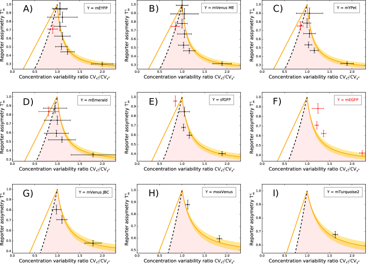
Figure 8: Utilizing constraints on flow-cytometry data from constitutively expressed fluorescent proteins. Here we plot all of the possible pairs from Table 1 in the Supplemental Material [34]. We plot 9 separate plots instead of combining the data into a single plot because for a given $T_{m}^{c}$ the right bound given by Eq. (8) is only determined if we specify one of the maturation times. Thus for fixed Y reporter, the right bound is well defined for any given X reporter, with the yellow corridor indicating the estimated uncertainty in $\tau_{c}$ and $\tau_{mat,y}$. Because all fluorescent proteins were constitutively expressed and were not fused to cellular proteins we expect the experimental data to be consistent with the class of gene expression models that do not exhibit feedback and are not periodically driven (pink region). All variability ratios with respect to all reference fluorescence proteins confirm the above picture with the exception for mEGFP (with ratios indicated in red) for which the data violate the expected behaviour. With the exception of the indicated mEGFP outlier all data fall along the right hand boundary.

Balleza et al. quantified the maturation dynamics of 50 different fluorescent proteins (FPs) in E. coli using time-lapse microscopy [15]. Their data show that the maturation step of roughly a third of the tested FPs are well described by first-order kinetics as assumed in our class of gene expression models. Additionally, the authors quantified heterogeneity in fluorescence levels when the respective FPs were expressed under the constitutive promoter proC. These data were obtained from flow-cytometry measurements of clonal E. coli MG1655 (CGSC 6300) populations in M9-rich media at 37^∘C. From their publicly available raw cell-to-cell heterogeneity data [36], we selected the ten FPs that were best modelled by first-order maturation kinetics (see Supplemental material [34]).

FP abundance CVs were obtained from the reported flow-cytometry fluorescence distributions. Under the assumption that reporter concentrations are cell-volume independent, i.e., transcription rates are cell-cycle independent, then the concentration CVs are related to the CVs in abundances and the CV in cell volume $CV_{V}$ [25]

$$CV_{\text{concentration}}^{2}=\frac{CV_{\text{abundance}}^{2}}{1+CV_{V}^{2}}-\frac{CV_{V}^{2}}{1+CV_{V}^{2}}.$$ (86)

We estimated $CV_{V}$ using separate time-lapse microscopy data that quantifies E. coli growth dynamics [37]. From the publicly available time-traces of E. coli length we computed an average volume variability of E. coli MG1655 (CGSC 6300) grown in LB media of $CV_{V}=0.261\pm 0.005$. The resulting concentration variability data are presented in Fig. 4C and a complete list of concentration CVs obtained this way along with the chosen FPs and their maturation times are presented in Table 1 in the Supplemental Material [34].

As shown in Fig. 8, all fluorescent protein pairs fall within the region expected for constitutively expressed genes, with the exception of mEGFP. The data fall along the right orange bound given by the right inequality in Eq. (8). According to Eq. (82), systems that lie along this boundary satisfy $CV_{x^{\prime\prime}_{c}}/CV_{y^{\prime\prime}_{c}}=\sqrt{\langle y^{\prime\prime}_{c}\rangle/\langle x^{\prime\prime}_{c}\rangle}$ where $x_{c}^{\prime\prime}$ and $y_{c}^{\prime\prime}$ denote the concentrations of the fluorescent proteins. Systems that lie along this bound thus have CVs that scale inversely with the square root of the averages. According to Eq. (84), the concentration CVs are given by

$$\begin{split}&CV_{x_{c}^{\prime\prime}}^{2}=\left\langle\frac{1}{V}\right\rangle\frac{1}{\langle x^{\prime\prime}_{c}\rangle}\\ &+\int_{0}^{\infty}\eta_{FF}A_{F_{x_{c}}}(t)\left(\frac{\tau_{mat,x}e^{-t/\tau_{mat,x}}-\tau_{c}^{\prime\prime}e^{-t/\tau_{c}^{\prime\prime}}}{\tau_{mat,x}^{2}-\tau_{c}^{\prime\prime 2}}\right)dt,\end{split}$$ (87)

where $F_{x_{c}}$ is the production rate of the immature protein concentrations. The first term on the right, which scales inversely to the average, corresponds to noise that originates at the translation step, the maturation step, fluctuations in protein degradation, and binomial splitting of proteins at cell division. The term on the right corresponds to noise that originates from transcription as well as mRNA and translation rate fluctuations. Therefor, data that lie along the right orange boundary in Fig. 8 corresponds to variability with negligible transcription noise contributions.

In order to confirm this observation and also analyze the mEGFP discrepancy, we plot in Fig. 8 the fluorescent protein concentration CVs as a function of their maturation times. In the regime where the the second term on the right of Eq. (87) is negligible, and where we assume that the fluorescent protein concentrations are degraded solely by dilution from the growing and dividing cells, we can use Eq. (82) to write

$$CV_{x_{c}^{\prime\prime}}=A\sqrt{\frac{\ln(2)}{\tau_{c}}\left(1+\text{ln}(2)\frac{\tau_{mat,x}}{\tau_{c}}\right)},$$ (88)

where $A=\sqrt{\left\langle\frac{1}{V}\right\rangle\frac{1}{\langle F\rangle}}$ is an unknown parameter. From this equation we see that as the maturation time gets larger, so does the CV. This is because as the maturation time gets larger, the fraction of matured proteins is reduced, which results in larger intrinsic fluctuations that originate from the maturation step and from cell partitioning of matured proteins. On the other hand, we can look at the regime in which there is negligible translation noise (where the second term on the right of Eq. (87) dominates). We model the autocorrelation of the protein concentration translation rate as a decaying exponential $A_{F_{x_{c}}}(t)=e^{-t/\tau_{F}}$, and we assume that the protein concentrations are degraded solely from dilution, in which case we have

$$CV_{x_{c}^{\prime\prime}}=B\sqrt{\frac{\tau_{F}(\tau_{c}^{\prime\prime}\tau_{x_{c}^{\prime}}+\tau_{F}(\tau_{c}^{\prime\prime}+\tau_{x_{c}^{\prime}}))}{(\tau_{F}+\tau_{c}^{\prime\prime})(\tau_{F}+\tau_{x_{c}^{\prime}})(\tau_{c}^{\prime\prime}+\tau_{x_{c}^{\prime}})}},$$ (89)

where $\tau_{c}^{\prime\prime}=\tau_{c}/\ln(2)$, $\tau_{x_{c}^{\prime}}=\left(1/\tau_{mat,x}+\ln(2)/\tau_{c}\right)^{-1}$, and $B=\sqrt{\eta_{FF}}$ is an unknown parameter. In Fig. 9 we plot Eq. (88) and Eq. (89) with $A=1.3$, $B=1.2$, $\tau_{F}=\tau_{c}/10$, and $\tau_{c}=28.5\pm 2$ min (as reported in [15]). We find that the computed CVs from the flow cytometry data sets are well described by Eq. (88), except for the mEGFP point which displays a CV smaller than the others. The only parameter left in this model to vary is the division time of the cells $\tau_{c}$. When this parameter is changed to $35.6$ min, the model captures the mEGFP data point as shown by the dashed curve in Fig. 9. The discrepancy between mEGFP and the other 9 fluorescent proteins could thus be explained by a slightly slower growth rate in the cell cultures used for the mEGFP data sets. The blue curve, on the other hand, corresponds to the negligible translation noise model given by Eq. (89). We find that as the maturation time gets larger, the CV gets smaller, which is expected as fluorescent proteins with large maturation times have less time to adjust to varying upstream fluctuations and inherit less variability.

The previous analysis indicates that the variability is dominated by noise originating from the translation step, maturation step, fluctuations in protein degradation, and noise originating from binomial splitting of protein numbers at cell divisions, which are all described by the first term on the right in Eq. (87). However, it is possible that measurement noise which scales inversely with the average is contributing to the measured variability. For example, in [25] it is shown that flow cytometry measurements contain a significant amount of measurement noise when used with bacteria due to their small size. This measurement noise is shown to scale inversely with the average of the fluorescence signal, meaning it could mask itself as biological variability contributing to the first term on the right of Eq. (87). In [25] a rigorous method is developed to measure the true CVs using flow cytometry on bacteria, separating measurement noise and autofluorescence contributions using commonly used calibration beads.

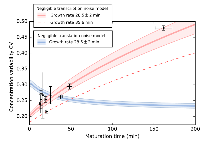
Figure 9: The data is best described by a model with negligible transcription noise. Plotted are the concentration CVs from Table 1 of the Supplemental Material [34] as a function of their respective fluorescent protein maturation times. The pink curve corresponds to the model given by Eq. (88) with $A=1.3$ and $\tau_{c}$ as reported in [15]: $28.5\pm 2$ min. The pink corridor indicates the result of the uncertainty in $\tau_{c}$. The blue curve corresponds to the model given by Eq. (89) in which translation noise is negligible, with $B=1.2$, $\tau_{F}=28.5/10$ min, and $\tau_{c}=28.5\pm 2$ min. We find that the data follows the pink curve and is thus best described by the negligible transcription noise model. The data point with the smallest CV corresponds to mEGFP, and the dashed red curve corresponds to the same model as the pink curve but with $\tau_{c}$ increased by a factor of 1.25. A possible explanation for this relatively low CV observed for mEGFP is that the cell cultures expressing mEGFP had slightly slower growth rates.

References

• Thattai and van Oudenaarden [2001] M. Thattai and A. van Oudenaarden, Intrinsic noise in gene regulatory networks, Proc. Natl. Acad. Sci. U. S. A. 98, 8614 (2001).
• Ozbudak et al. [2002] E. M. Ozbudak, M. Thattai, I. Kurtser, A. D. Grossman, and A. van Oudenaarden, Regulation of noise in the expression of a single gene, Nat. Genet. 31, 69 (2002).
• Blake et al. [2003] W. J. Blake, M. Kærn, C. R. Cantor, and J. J. Collins, Noise in eukaryotic gene expression, Nature 422, 633 (2003).
• Bar-Even et al. [2006] A. Bar-Even, J. Paulsson, N. Maheshri, M. Carmi, E. O’Shea, Y. Pilpel, and N. Barkai, Noise in protein expression scales with natural protein abundance, Nat. Genet. 38, 636 (2006).
• Newman et al. [2006] J. R. Newman, S. Ghaemmaghami, J. Ihmels, D. K. Breslow, M. Noble, J. L. DeRisi, and J. S. Weissman, Single-cell proteomic analysis of S. cerevisiae reveals the architecture of biological noise, Nature 441, 840 (2006).
• Eldar and Elowitz [2010] A. Eldar and M. B. Elowitz, Functional roles for noise in genetic circuits, Nature 467, 167 (2010).
• Jones and Elf [2018] D. Jones and J. Elf, Bursting onto the scene? Exploring stochastic mRNA production in bacteria, Current Opinion in Microbiology 45, 124 (2018).
• Kærn et al. [2005] M. Kærn, T. C. Elston, W. J. Blake, and J. J. Collins, Stochasticity in gene expression: from theories to phenotypes, Nature Reviews Genetics 6, 451 (2005).
• Hilfinger et al. [2016a] A. Hilfinger, T. M. Norman, and J. Paulsson, Exploiting natural fluctuations to identify kinetic mechanisms in sparsely characterized systems, Cell Systems 2, 251 (2016a).
• Taniguchi et al. [2010] Y. Taniguchi, P. J. Choi, G.-W. Li, H. Chen, M. Babu, J. Hearn, A. Emili, and X. S. Xie, Quantifying E. coli proteome and transcriptome with single-molecule sensitivity in single cells., Science 329, 533 (2010).
• Lubeck et al. [2014] E. Lubeck, A. F. Coskun, T. Zhiyentayev, M. Ahmad, and L. Cai, Single-cell in situ RNA profiling by sequential hybridization, Nat Meth 11, 360 (2014).
• Elowitz et al. [2002] M. B. Elowitz, A. J. Levine, E. D. Siggia, and P. S. Swain, Stochastic gene expression in a single cell, Science 297, 1183 (2002).
• Raser and O’Shea [2004] J. M. Raser and E. K. O’Shea, Control of stochasticity in eukaryotic gene expression, Science 304, 1811 (2004).
• Maamar et al. [2007] H. Maamar, A. Raj, and D. Dubnau, Noise in gene expression determines cell fate in Bacillus subtilis, Science 317, 526 (2007).
• Balleza et al. [2018] E. Balleza, J. Mark Kim, and P. Cluzel, Systematic characterization of maturation time of fluorescent proteins in living cells, Nature Methods 15, 47 (2018).
• Shen-Orr et al. [2002] S. S. Shen-Orr, R. Milo, S. Mangan, and U. Alon, Network motifs in the transcriptional regulation network of Escherichia coli, Nature genetics 31, 64 (2002).
• Baudrimont et al. [2019] A. Baudrimont, V. Jaquet, S. Wallerich, S. Voegeli, and A. Becskei, Contribution of RNA degradation to intrinsic and extrinsic noise in gene expression, Cell reports 26, 3752 (2019).
• Hilfinger et al. [2016b] A. Hilfinger, T. M. Norman, G. Vinnicombe, and J. Paulsson, Constraints on fluctuations in sparsely characterized biological systems, Phys. Rev. Lett. 116, 058101 (2016b).
• Raj et al. [2006] A. Raj, C. S. Peskin, D. Tranchina, D. Y. Vargas, and S. Tyagi, Stochastic mRNA synthesis in mammalian cells, PLoS Biol 4, e309 (2006).
• Skinner et al. [2013] S. O. Skinner, L. A. Sepúlveda, H. Xu, and I. Golding, Measuring mRNA copy number in individual Escherichia coli cells using single-molecule fluorescent in situ hybridization, Nature protocols 8, 1100 (2013).
• Eling et al. [2019] N. Eling, M. D. Morgan, and J. C. Marioni, Challenges in measuring and understanding biological noise, Nature Reviews Genetics 20, 536 (2019).
• Emory et al. [1992] S. A. Emory, P. Bouvet, and J. G. Belasco, A 5’-terminal stem-loop structure can stabilize mRNA in Escherichia coli, Genes & development 6, 135 (1992).
• Cheneval et al. [2010] D. Cheneval, T. Kastelic, P. Fuerst, and C. N. Parker, A review of methods to monitor the modulation of mRNA stability: a novel approach to drug discovery and therapeutic intervention, Journal of Biomolecular screening 15, 609 (2010).
• Shaffer et al. [2013] S. M. Shaffer, M.-T. Wu, M. J. Levesque, and A. Raj, Turbo FISH: a method for rapid single molecule RNA FISH, PLoS One 8, e75120 (2013).
• Galbusera et al. [2020] L. Galbusera, G. Bellement-Theroue, A. Urchueguia, T. Julou, and E. van Nimwegen, Using fluorescence flow cytometry data for single-cell gene expression analysis in bacteria, PloS One 15, e0240233 (2020).
• Grün et al. [2014] D. Grün, L. Kester, and A. Van Oudenaarden, Validation of noise models for single-cell transcriptomics, Nature methods 11, 637 (2014).
• Raj et al. [2008] A. Raj, P. Van Den Bogaard, S. A. Rifkin, A. Van Oudenaarden, and S. Tyagi, Imaging individual mRNA molecules using multiple singly labeled probes, Nature methods 5, 877 (2008).
• Eng et al. [2019] C.-H. L. Eng, M. Lawson, Q. Zhu, R. Dries, N. Koulena, Y. Takei, J. Yun, C. Cronin, C. Karp, G.-C. Yuan, et al., Transcriptome-scale super-resolved imaging in tissues by RNA seqFISH+, Nature 568, 235 (2019).
• Rhee et al. [2014] A. Rhee, R. Cheong, and A. Levchenko, Noise decomposition of intracellular biochemical signaling networks using nonequivalent reporters, Proceedings of the National Academy of Sciences 111, 17330 (2014).
• Van Kampen [1992] N. G. Van Kampen, Stochastic processes in physics and chemistry, Vol. 1 (Elsevier, 1992).
• Lestas et al. [2008] I. Lestas, J. Paulsson, N. E. Ross, and G. Vinnicombe, Noise in gene regulatory networks, IEEE Trans. Automat. Contr. 53, 189 (2008).
• Hilfinger and Paulsson [2011] A. Hilfinger and J. Paulsson, Separating intrinsic from extrinsic fluctuations in dynamic biological systems, Proc. Natl. Acad. Sci. U. S. A. 108, 12167 (2011).
• Hilfinger et al. [2012] A. Hilfinger, M. Chen, and J. Paulsson, Using temporal correlations and full distributions to separate intrinsic and extrinsic fluctuations in biological systems, Phys. Rev. Lett. 109, 248104 (2012).
• [34] See supplemental material attached to the end of the manuscript.
• Davenport et al. [1958] W. B. Davenport, W. L. Root, et al.An introduction to the theory of random signals and noise, Vol. 159 (McGraw-Hill New York, 1958).
• Balleza [2017] E. Balleza, Flow Cytometry Data, Harvard Dataverse https://doi.org/10.7910/DVN/T4VSGH (2017).
• Wang et al. [2010] P. Wang, L. Robert, J. Pelletier, W. L. Dang, F. Taddei, A. Wright, and S. Jun, Robust growth of escherichia coli, Current biology 20, 1099 (2010).