Constraining the Cosmic Baryon Distribution with Fast Radio Burst Foreground Mapping

Abstract

The dispersion measures (DM) of fast radio bursts (FRBs) encode the integrated electron density along the line-of-sight, which is typically dominated by the intergalactic medium (IGM) contribution in the case of extragalactic FRBs. In this paper, we show that incorporating wide-field spectroscopic galaxy survey data in the foreground of localized FRBs can significantly improve constraints on the partition of diffuse cosmic baryons. Using mock DMs and realistic lightcone galaxy catalogs derived from the Millennium simulation, we define spectroscopic surveys that can be carried out with 4m and 8m-class wide field spectroscopic facilities. On these simulated surveys, we carry out Bayesian density reconstructions in order to estimate the foreground matter density field. In comparison with the ‘true’ matter density field, we show that these can help reduce the uncertainties in the foreground structures by $\sim 2-3\times$ compared to cosmic variance. We calculate the Fisher matrix to forecast that $N=30\>(96)$ localized FRBs should be able to constrain the diffuse cosmic baryon fraction to $\sim 10\%\>(\sim 5\%)$, and parameters governing the size and baryon fraction of galaxy circumgalactic halos to within $\sim 20-25\%\>(\sim 8-12\%)$. From the Fisher analysis, we show that the foreground data increases the sensitivity of localized FRBs toward our parameters of interest by $\sim 25\times$. We briefly introduce FLIMFLAM, an ongoing galaxy redshift survey that aims to obtain foreground data on $\sim 30$ localized FRB fields.

1 Introduction

The “missing baryon problem” has been, since the turn of the millennium, one of the major unsolved problems in astrophysics (see, e.g., Fukugita & Peebles 2004; Cen & Ostriker 2006; Bregman 2007). Despite strong constraints on $\Omega_{\mathrm{b}}$, the cosmic baryon fraction, from Big Bang nucleosynthesis and cosmic microwave background experiments (Planck Collaboration et al., 2020), observations of the low-redshift Universe ($z\lesssim 1$) have persistently failed to account for the same amount of baryonic matter. Stars, interstellar medium (ISM) gas in galaxies, and hot X-ray-emitting gas in galaxy clusters only account for $\sim 10\%$ of the primordial baryon fraction (e.g., Persic & Salucci, 1992; Fukugita et al., 1998), indicating the rest must reside in the intergalactic medium (IGM) or circum-galactic medium (CGM).

The baryons in the CGM and IGM at $z\gtrsim 2$ are largely accounted for in the observed population of H I Lyman-$\alpha$ absorbers, thanks to the relatively simple astrophysics of photoionization equilibrium embedded in quasi-linear structure formation. However, the IGM at $z<1$ is strongly affected by gravitational shock-heating and feedback from galaxy formation. This leads to a complex multi-phase medium at low redshifts (Cen & Ostriker, 2006; Smith et al., 2011), much of which evade easy detection by either X-ray emission or absorption line tracers. Heroic efforts in recent years have uncovered part of the missing baryon budget via a plethora of techniques, ranging from H I Lyman-$\alpha$ absorption (Danforth & Shull, 2008); high-ionization metal absorption (Prochaska et al., 2011; Nicastro et al., 2018), stacked X-ray emission in filaments (Tanimura et al., 2020), to the Sunyaev-Zel’dovich effect (Tanimura et al., 2019a, b; Lim et al., 2020). Nevertheless, as of 2020, as much as $\sim 20\%$ of the cosmic baryons remained unaccounted for, and it was also the case that no single method could account for more than $\sim 20-30\%$ of the baryon budget.

The burgeoning field of fast radio burst (FRB) research over the past decade has opened a promising new avenue towards addressing the missing baryon problem. Detected as millisecond transient radio pulses (see Cordes & Chatterjee 2019 for a comprehensive review of the FRB phenomenon), FRB signals exhibit a time arrival difference between photons of different frequencies — usually termed the ‘dispersion measure’ (DM) — caused by free electrons along the line-of-sight to the FRB, $\mathrm{DM}=\int n_{\mathrm{e}}/(1+z)\,\mathrm{d}s$, where $s$ is the proper line element. The overall DM signal from an FRB at redshift $z_{\mathrm{frb}}$ is thought to arise from several contributions:

$$\mathrm{DM}_{\mathrm{FRB}}=\mathrm{DM}_{\mathrm{MW}}+\mathrm{DM}_{\mathrm{igm}}+\mathrm{DM}_{\mathrm{halos}}+\frac{\mathrm{DM}_{\mathrm{host}}}{1+z_{\mathrm{frb}}},$$ (1)

where $\mathrm{DM}_{\mathrm{MW}}$ is the contribution from the Milky Way’s interstellar medium and halo gas, $\mathrm{DM}_{\mathrm{igm}}$ arises from the diffuse intergalactic medium gas tracing the cosmic large-scale structure on $\geq$Mpc-scales, $\mathrm{DM}_{\mathrm{halos}}$ is from the aggregate intervening galaxy halo gas within several arcmin (tens of transverse kpc) of the sightline, and $\mathrm{DM}_{\mathrm{host}}$ is from the host galaxy and progenitor source.

The large DM values observed in FRBs compared to galactic pulsars (Manchester et al., 2005) were a key piece of evidence pointing at their extragalactic origin, as the requisite integrated electron contributions are likely only to arise from a long extragalactic path through an ionized medium (Lorimer et al., 2007). With the reasonable approximation that all intergalactic and circumgalactic gas is ionized, the extragalactic DM is thus a probe of all the cosmic baryons, regardless of the exact phase of the gas (McQuinn, 2014).

Even though $>600$ FRBs have now been detected at the time of writing (e.g., Petroff et al., 2016; The CHIME/FRB Collaboration et al., 2021), there are several uncertainties that need to be overcome in order to use FRBs to probe the cosmic baryon distribution. While there should exist, on average, a monotonic relationship between the extragalactic DM contribution and the redshift of the FRB (Ioka, 2003; Inoue, 2004; McQuinn, 2014; Pol et al., 2019), the redshift of the FRB needs to be measured in order to anchor constraints that relate models of the cosmic baryon distribution to the resulting DM. In practice, this requires first measuring the position of the FRB to sufficient accuracy ($\sim$ arcsecond) in order to associate it with a host galaxy, and then measuring the host galaxy’s spectroscopic redshift. With the first generation of FRB surveys conducted primarily using large single-dish radio telescopes such as Parkes (also known as Murriyang), Arecibo, or the Green Bank Telescope, FRB positions could only be measured to within several arcminutes — error circles within which hundreds of galaxies could be the FRB host.

The discovery of repeating FRBs (Spitler et al., 2016) enabled the first localizations of FRBs to specific host galaxies thanks to follow-up observations with interferometric arrays. However, repeating FRBs appear to comprise only a small fraction of all observed FRBs (CHIME/FRB Collaboration et al., 2019; James et al., 2020), possibly representing a different source population (e.g., Hashimoto et al., 2020; Heintz et al., 2020), and by nature are time-consuming to confirm and follow-up. The numbers of repeating FRBs that can be accurately localized to host galaxies therefore are low, and will take time to build up significant samples that can be used for studies of the cosmic baryons.

Instead, wide-field interferometric arrays such as the Australian Square Kilometre Array Pathfinder (ASKAP; McConnell et al., 2016; Shannon et al., 2018) and the Deep Synoptic Array (DSA; Kocz et al., 2019) are starting to detect FRBs with sufficient resolution ($\sim 0.1-1\arcsec$) to match a plausible host galaxy within the error circle of the localization (e.g., Bannister et al., 2019; Bhandari et al., 2020; Ravi et al., 2019). Using a sample of six FRBs that had been localized with ASKAP and subsequent redshift measurements of the host galaxies, Macquart et al. (2020) demonstrated that the extragalactic DMs of these FRBs follow a DM-$z$ relationship that is consistent with the cosmic baryon fraction, $\Omega_{\mathrm{b}}$, expected from the standard $\Lambda$CDM cosmology — the so-called “Macquart Relation”.

While the cosmic baryons are no longer “missing” thanks to the Macquart et al. (2020) result (complemented by techniques probing denser gas, e.g. Werk et al., 2014; Nicastro et al., 2018) many questions remain regarding their distribution in the Universe. For example, the partition between the diffuse cosmic web baryons and circumgalactic halo gas is currently unknown, as well as the spatial extent of CGM gas beyond their host galaxies. This question is reflected by the scatter in the Macquart Relation, in which the extragalactic DM at fixed FRB redshift exhibits a variance from the diversity of possible paths through over- and under-densities in the intergalactic medium, as well as the possibility of intersecting foreground galaxy or cluster halos. This scatter causes significant uncertainty in efforts to determine, for example, the fraction of cosmic baryons in the diffuse cosmic web as opposed to the CGM.

Walters et al. (2019) forecasted constraints on $f_{\mathrm{igm}}$, the fraction of cosmic baryons residing in the diffuse cosmic web, from observational samples of localized FRBs, and concluded that samples of $N\sim[100,1000]$ would be required to place $\sigma\sim[5\%,2\%]$ constraints in combination with existing cosmological probes. More observational information would allow tighter constraints on the cosmic baryon distribution: Ravi (2019) argued that spectroscopic observations of foreground galaxies near FRB sightlines would allow $\sim 2\%$ constraints on $f_{\mathrm{igm}}$ with samples of $\sim 50$ localized FRBs. However, we note that both Walters et al. (2019) and Ravi (2019) appear to have underestimated the scatter arising from the diffuse cosmic web by adopting $\sigma_{\mathrm{igm}}\approx 10\,\mathrm{pc}\,\mathrm{cm}^{-3}$. This is a factor of $\sim 3-10\times$ smaller than the corresponding quantity seen in hydrodynamical simulations (e.g., Jaroszynski, 2019; Takahashi et al., 2020), which make the forecasts in Walters et al. (2019) and Ravi (2019) too optimistic; this despite the fact that they already call for large numbers of localized FRBs, a number unlikely to be achieved in the next 5 years. In other words, even with large samples of localized FRBs, large-scale variance caused by the density fluctuations in the FRB foreground causes significant uncertainty in the cosmic baryon census that can be achieved using FRB lines-of-sight.

In this paper, we will argue that wide-field galaxy redshift surveys (covering several square degrees) targeted at the foreground of localized FRBs will allow us to address this sightline variance and make precision constraints on the cosmic baryon distribution. Simha et al. (2020) has carried out a preliminary implementation of this idea using spectroscopic data from the Sloan Digital Sky Survey (SDSS; Blanton et al., 2005; Abazajian et al., 2009) in front of the $z=0.1167$ FRB190608 (Chittidi et al., 2020), although their analysis was very limited by the statistical power offered by just one FRB. Assuming that expanded data sets consisting of dozens of localized FRBs and their foreground data will become available over the next few years, we will demonstrate an approach that can be used to make precise constraints on the cosmic baryon distribution. We will aim, in particular, to outline the numbers of galaxies and apparent magnitudes that would be needed to map out each FRB foreground field at various redshifts, in order to demonstrate that the technique is viable with existing and upcoming multiplexed spectroscopic facilities.

This paper is organized as follows: Section 2 will describe the simulations that we will use as a basis for our forecasts; Section 3 will describe how we set up the mock observations that we will subsequently analyze; Section 4 will describe the reconstruction algorithm used to estimate the density field from the foreground data, which will then feed into the parameter estimation and forecasts in Section 5. Finally, in Section 6 we will give a preliminary description of FLIMFLAM, a newly-initiated spectroscopic survey that aims to implement the techniques introduced in this paper.

2 Simulations

In this paper, we perform mock analyses on redshift catalogs and density fields derived from numerical simulations in order to forecast the constraints on the cosmic baryon distribution in front of localized FRBs. Specifically, we use the Millennium N-body simulations (Springel, 2005) and the associated semi-analytic lightcone catalogs from Henriques et al. (2015), referred to hereafter H15.

Briefly, the H15 lightcone catalog is based the Millennium N-body simulation (Springel, 2005) which was run with $2160^{3}$ particles within a box size of $L=500\,h^{-1}\,\mathrm{Mpc}$ per side, using the smoothed particle hydrodynamics code GADGET-2 (Springel et al., 2005). To rescale the original simulation to be more consistent with the Planck13 cosmology (Planck Collaboration et al., 2014), H15 applied the technique of Angulo & Hilbert (2015) which modified the effective box size from $L=500\,h^{-1}\,\mathrm{Mpc}$ to $L=480.279\,h^{-1}\,\mathrm{Mpc}$ and relabeled several of the snapshot redshifts in order to better match the evolution of structure as expected from the Planck13 cosmology.

On the rescaled Millennium N-body data, H15 implemented an updated version of the “Munich” semi-analytic galaxy formation model (Guo et al. 2011). This involved changes to the modelling of various phenomena such as the star-formation thresholds, wind re-accretion, radio-mode feedback, stellar populations and models. The 17 free parameters in the semi-analytic model were then tuned to match a set of observational data out to $z\sim 3$, in particular the abundances and passive fractions of galaxies in the stellar mass range $8.0\leq\log M_{\star}/M_{\odot}\leq 12.0$. They then calculated the galaxy rest-frame spectral energy distributions assuming two different stellar population synthesis models; in this paper, we use the H15 catalogs generated with the Maraston (2005) models.

Lightcone catalogs were then generated using a method first introduced by Blaizot et al. (2005), namely by calculating the coordinates and multi-wavelength apparent photometry of the galaxies as ‘observed’ from several cartesian origin points and random viewing angles in the simulation grid. They also used a method introduced by Kitzbichler & White (2007) to chose the line-of-sight direction in order to minimize repetitions of the same object within the lightcone as it periodically wraps through different simulation snapshots. There were 24 separate lightcones each with a $\pi\,\mathrm{deg}^{2}\simeq 3.14\,\mathrm{deg}^{2}$ field-of-view reaching to $z\sim 4$, as well as two “all-sky” lightcones that cover $4\pi$ steradian around the chosen origins but are limited to galaxies with apparent magnitudes of $i<21$. In this work, we will primarily use six of the $\pi$-square degree lightcones that share the same simulation coordinate origins as the “all-sky” catalogs in order to simultaneously simulate wide-surveys like 6dF or SDSS in conjunction with deeper dedicated spectroscopic observations. For each of the narrow $\pi$-square degree lightcones, we downloaded the galaxy catalogs for $z<1.2$ objects down to a limiting halo mass of $M_{\mathrm{vir}}\geq 3\times 10^{11}\,M_{\odot}$, while for the all-sky lightcones we downloaded the full $i<21$ catalog.

Following H15, we will use the Planck13 cosmology throughout this paper: $\sigma_{8}=0.829$, $H_{0}=67.3\,\mathrm{km}\,\mathrm{s}^{-1}\mathrm{Mpc}^{-1}$, $h=H_{0}/(100\,\mathrm{km}\,\mathrm{s}^{-1}\mathrm{Mpc}^{-1})=0.673$, $\Omega_{\Lambda}=0.685$, $\Omega_{m}=0.315$, $\Omega_{b}=0.0487$, and $n=0.96$ (Planck Collaboration et al., 2014). These cosmological parameters are no longer up-to-date, but for the purposes of our mock analyses this is not an issue so long as we remain internally consistent.

3 Mock Observables

There are two overall components to the mock observations that we generate from the H15 lightcone and density field. The first is the cosmic dispersion measure traced along a given sightline of the lightcone, which would be directly measured as part the initial FRB observation. The second component we consider is the spectroscopic galaxy samples that need to be obtained as part of a dedicated observational program on optical telescopes (although some partial data might already exist from prior wide-field surveys).

First, we select an ‘FRB’ at the desired redshift $z_{\mathrm{frb}}$ by randomly choosing a halo with the correct redshift from one of the H15 lightcone catalogs, that has a central halo virial mass of $M_{\mathrm{vir}}>3\times 10^{10}\,M_{\odot}$ or apparent magnitude of $i<23$. This is a somewhat arbitrary cut, but goes to sufficiently low masses and luminosities to reflect the fact that FRB host galaxies seem to span a wide range in properties (e.g. Heintz et al., 2020). We also ensure that each FRB position is at least 3 arcmin from any other FRB sightline selected within the same lightcone, in order to minimize correlations between adjacent lines-of-sight.

Secondly, we will define the mock spectroscopic samples of the foreground galaxies observed in front of each FRB. These need to be at different depths and areal densities in order to probe different redshifts, and we will also describe the observational requirements needed to achieve these samples.

3.1 FRB Dispersion Measures

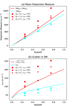
Figure 1: Cosmic dispersion measure statistics compared between our models (symbols) against those from the Illustris hydrodynamical simulations analyzed by J19 (solid curves). Red curves and symbols indicate the combined IGM and halo quantities, while cyan is for the IGM only. In the top panel (a), changes in our model parameters do not significantly modify the mean DM values, which are generally consistent with J19. At bottom (panel (b)), the scatter in the IGM contribution is affected by the Gaussian smoothing length, $R_{sm}$, applied to the matter field in our model. We will adopt the $R_{sm}$ value which best matches the $\sigma_{\mathrm{igm}}$ in J19. In this figure, $f_{\mathrm{igm}}=0.85$ is assumed in our models, while $R_{sm}$ and $r_{\mathrm{max}}$ in the legends are quoted in units of $h^{-1}\,\mathrm{Mpc}$ and $r_{200}$, respectively.

The first mock observable we need to define is the dispersion measure that is measured as part of the initial FRB detection in the radio.

We will separately calculate $\mathrm{DM}_{\mathrm{igm}}$, $\mathrm{DM}_{\mathrm{halos}}$, and $\mathrm{DM}_{\mathrm{host}}$ contributions that would be observed for a simulated FRB sightline within the simulation. First, we will define as the primary observable for our analysis, the extragalactic DM component:

$$\mathrm{DM}_{\mathrm{eg}}=\mathrm{DM}_{\mathrm{FRB}}-\mathrm{DM}_{\mathrm{MW}},$$ (2)

which represents all the DM contributions from beyond the Milky Way and its halo. $\mathrm{DM}_{\mathrm{eg}}$ will therefore constitute one of the key observables in our subsequent forecast:

$$\mathrm{DM}_{\mathrm{eg}}=\mathrm{DM}_{\mathrm{igm}}+\mathrm{DM}_{\mathrm{halos}}+\frac{\mathrm{DM}_{\mathrm{host}}}{1+z_{\mathrm{frb}}}+\delta_{N},$$ (3)

where a random deviate arising from noise and Milky Way subtraction, $\delta_{N}$, has also been added.

To compute the $\mathrm{DM}_{\mathrm{igm}}$ component arising from large-scale IGM, we use the gridded $256^{3}$ Millennium density field snapshots with a side length of $L=480.279\,h^{-1}\,\mathrm{Mpc}$, that we smoothed with a Gaussian kernel with size $R_{sm}$. First, we computed the path between the FRB coordinate and lightcone origin, keeping track of the exact path length $l_{s}$ traced by the sightline through each grid cell $s$ as well as the redshift $z_{i}$ at to the simulation snapshot corresponding to the line-of-sight comoving distance from the origin for the traversed cell. We calculate a discretized version of $\mathrm{DM}_{\mathrm{igm}}=\int n_{e}^{\mathrm{igm}}/(1+z)\,\mathrm{d}s$ as follows:

$$\mathrm{DM}_{\mathrm{igm}}=\bar{n}_{e}^{\mathrm{igm}}(z_{i})\sum\limits_{s}(1+\delta^{sm}_{m,s})\,l_{s}(1+z_{s})^{-1},$$ (4)

where is $\delta^{sm}_{m,s}$ and $l_{s}$ are the smoothed matter overdensity and path length through the grid cell $s$, respectively; $z_{s}$ is the redshift of the grid cell calculated from the distance-redshift relation, and $\bar{n}_{e}^{\mathrm{igm}}$ is the mean cosmic electron density at the redshift of the snapshot $z_{i}$, defined as:

$$\bar{n}_{e}^{\mathrm{igm}}(z_{i})=f_{\mathrm{igm}}\Omega_{\mathrm{b}}\bar{\rho_{c}}(z_{i})\left[\frac{m_{\mathrm{He}}(1-Y)+2Ym_{\mathrm{H}}}{m_{\mathrm{H}}m_{\mathrm{He}}}\right],$$ (5)

where $m_{\mathrm{H}}$ and $m_{\mathrm{He}}$ are the atomic masses of hydrogen and helium, respectively; $Y=0.243$ is the cosmic mass fraction in helium (assumed to be double-ionized); $\Omega_{\mathrm{b}}=0.044$ is the fraction of the cosmic critical density in baryons, $\bar{\rho}_{c}(z_{i})$ is the critical density of the universe at the redshift $z_{i}$, and $f_{\mathrm{igm}}$ is the fraction of cosmic baryons residing in the diffuse IGM. The summation carried out in Equation 4 traverses different density snapshots of the Millennium simulation according to the snapshot redshift $z_{s}$ which is closest to the cell redshift $z_{i}$: for example, a sightline originating at $z_{\mathrm{frb}}=0.5$ would pass through 14 different redshift snapshots.

Next, we calculate the $\mathrm{DM}_{\mathrm{halos}}$ contribution from intervening galaxy halos close to the FRB line-of-sight, assuming that the halo gas is described by a modified Navarro-Frank-White (mNFW) profile as elucidated in Prochaska & Zheng (2019). The baryon density as a function of radius is given by:

$$\rho_{\mathrm{b}}=\frac{\rho^{0}_{\mathrm{b}}}{y^{1-\alpha}(y_{0}+y)^{2+\alpha}},$$ (6)

where $\rho^{0}_{\mathrm{b}}$ is the central density, $y$ is a rescaled radius (see Mathews & Prochaska 2017 for the full definitions), and we fix the profile parameters $\alpha=2$ and $y_{0}=2$. This choice of parameters is designed to produce halo gas profiles similar to those derived by Maller & Bullock (2004) for multi-phase circumgalactic media. For a halo with mass $M_{\mathrm{halo}}$, the total mass in baryons is:

$$M_{\mathrm{halo}}^{b}\equiv f_{\mathrm{hot}}(\Omega_{b}/\Omega_{m})M_{\mathrm{halo}},$$ (7)

where $f_{\mathrm{hot}}$ represents the fraction of the halo baryons that are in a hot gas phase tracing the mNFW profile out to 1 virial radius. We truncate the mNFW profile at a given radius $r_{\mathrm{max}}$, which is usually of comparable magnitude to the virial radius $r_{200}$, and so we will usually quote $r_{\mathrm{max}}$ in units of $r_{200}$. Simha et al. (2020) showed that varying the assumed $r_{\mathrm{max}}$ for the foreground galaxies of FRB190608 from $r_{200}$ to $2\times r_{200}$ more than doubled the $\mathrm{DM}_{\mathrm{halos}}$ contribution, so this will be one of the free parameters that we will consider in our mock analysis.

To speed up the computation we only calculate the $\mathrm{DM}_{\mathrm{halos}}$ contribution for foreground galaxies within $10^{\prime}$ of each simulated FRB sightline. This corresponds approximately to the transverse separation at $r_{200}$ of a $10^{13}\,M_{\odot}$ halo at $z=0.05$ — for lower-mass or higher redshift halos, the transverse extent $r_{200}$ will be correspondingly smaller. Since we are defining our mock observables at this point, there is no possibility of halos outside of this separation biasing our forecast so long as we remain internally consistent. In a real observation, we would have to carefully consider the possible contributions of more massive, cluster-sized, halos that might contribute at larger transverse separations if they are low redshift. In this regime, $\mathrm{DM}_{\mathrm{halos}}$ and $\mathrm{DM}_{\mathrm{igm}}$ will begin to overlap as group- and cluster-sized halos will also represent clear overdensities on $\sim$Mpc-scales. When analyzing real observations, we will need to carefully keep track of these massive halos to avoid double-counting their DM contributions, but in our mock analysis the separation is clear. This is because both mock ‘observations’ and fitting functions are derived from exactly the same model as described in this section.

In addition to computing the $\mathrm{DM}_{\mathrm{halos}}$ for each sightline, we also output a catalog listing the redshift, separation, halo mass, and DM contribution of all galaxies at $<10\arcmin$ within each sightline. This will be used in the subsequent Fisher matrix parameter forecast.

Now that we have defined $\mathrm{DM}_{\mathrm{igm}}$ and $\mathrm{DM}_{\mathrm{halos}}$, we will remark on the effect of the Gaussian smoothing length, $R_{sm}$, applied to the N-body density field before calculating $\mathrm{DM}_{\mathrm{igm}}$ from Equation 4. In principle, at fixed cosmology and for a given cosmic baryon distribution, there is no effect from varying $R_{sm}$ on $\langle\mathrm{DM}_{\mathrm{igm}}+\mathrm{DM}_{\mathrm{halos}}\rangle(z)$ (i.e. the IGM and halo dispersions averaged over the Universe at fixed FRB redshift). However, the scatter in $\mathrm{DM}_{\mathrm{igm}}$, which we refer to as $\sigma_{\mathrm{igm}}$, will vary as a function of $R_{sm}$ — with large $R_{sm}$ the variance in $\mathrm{DM}_{\mathrm{igm}}$ between different sightlines will get washed out. As a comparison, we use the results of Jaroszynski (2019), hereafter J19, who studied the statistics of the $\mathrm{DM}_{\mathrm{igm}}$ distribution in the Illustris cosmological hydrodynamical simulations (see also Takahashi et al. 2020; Zhu & Feng 2020; Zhang et al. 2021, Batten et al. 2021b). We calculated $\langle\mathrm{DM}_{\mathrm{igm}}\rangle(z)$ at several redshifts using our model (Equation 4), for a few different values of $R_{sm}$. In each case, we averaged over 750 sightlines drawn from the 24 separate H15 lightcones, and set $f_{\mathrm{igm}}=0.85$ to match the average $z<1$ value found by J19. The $\langle\mathrm{DM}_{\mathrm{igm}}\rangle(z)$ from our models are shown as cyan symbols in Figure 1a, in comparison with the J19 $\mathrm{DM}_{\mathrm{igm}}$ curve shown as a cyan line.

Our model — derived from the density field of the non-hydrodynamical Millennium simulation — has a reasonable agreement with J19, and as expected varying $R_{sm}$ does not significantly modify $\langle\mathrm{DM}_{\mathrm{igm}}\rangle(z)$.

We also computed $\langle\mathrm{DM}_{\mathrm{igm}}+\mathrm{DM}_{\mathrm{halos}}\rangle(z)$ (red symbols in Figure 1a) for a range of $[r_{\mathrm{max}},R_{sm}]$, which does exhibit significant changes with respect to parameter choice. Since $\langle\mathrm{DM}_{\mathrm{igm}}(z)\rangle$ alone shows little variation respect to $R_{sm}$, this variation in $\langle\mathrm{DM}_{\mathrm{igm}}+\mathrm{DM}_{\mathrm{halos}}\rangle(z)$ must come from the response of $\mathrm{DM}_{\mathrm{halos}}$ with respect to $r_{\mathrm{max}}$. For some of the larger values of $r_{\mathrm{max}}$, the overall $\langle\mathrm{DM}_{\mathrm{igm}}+\mathrm{DM}_{\mathrm{halos}}\rangle(z)$ becomes large enough that it exceeds the total baryon budget of the Universe. However, in this paper we will treat $r_{\mathrm{max}}$ as a free parameter for our forecast, therefore we will not seek to match $r_{\mathrm{max}}$ with J19 or any other hydrodynamical simulation. However, we note in passing that this comparison with J19 implies that the halo CGM in the Illustris simulation has characteristic scales of comparable to the halo virial radius.

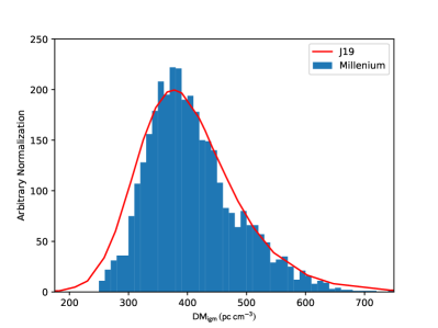
Figure 2: Distribution of $\mathrm{DM}_{\mathrm{igm}}$ at $z=0.5$, shown for both our model with $R_{sm}=0.7\,h^{-1}\,\mathrm{Mpc}$ (histogram) as well as that from J19 (red curve). Our model provides a reasonable match with that from the hydrodynamical simulation. The mean and scatter for our model distribution shown here is $\langle\mathrm{DM}_{\mathrm{igm}}=412\,\mathrm{pc}\,\mathrm{cm}^{-3}$ and $\sigma_{\mathrm{igm}}=79\,\mathrm{pc}\,\mathrm{cm}^{-3}$.

The scatter of the $\mathrm{DM}_{\mathrm{igm}}$ distribution (Figure 1b), however, shows considerably more variation with respect to the choice of parameters in our model, especially with respect to $R_{sm}$. Given the cell size of $1.875\,h^{-1}\,\mathrm{Mpc}$ in the Millennium binned density field, we find that Gaussian smoothing by $R_{sm}=0.7\,h^{-1}\,\mathrm{Mpc}$ provides an adequate match for $\sigma_{\mathrm{igm}}$ in our model in comparison with J19. In Figure 2, we show the probability distribution of $\mathrm{DM}_{\mathrm{igm}}$ only computed at $z=0.5$ both for our model, and that from the Illustris hydrodynamical simulation by J19. We have set $R_{sm}=0.7\,h^{-1}\,\mathrm{Mpc}$ and $f_{\mathrm{igm}}=0.85$ to get the best match with J19. The two distributions are similar, with a long non-Gaussian tail toward high $\mathrm{DM}_{\mathrm{igm}}$, although the J19 distribution extends toward lower $\mathrm{DM}_{\mathrm{igm}}$ compared with ours.

Note that these $\sigma_{\mathrm{igm}}$ values, in both our model and J19, are higher at all redshifts than the $\sigma_{\mathrm{igm}}=10\,\mathrm{pc}\,\mathrm{cm}^{-3}$ adopted by Walters et al. (2019) and Ravi (2019). Considering the variance in both $\mathrm{DM}_{\mathrm{igm}}$ and $\mathrm{DM}_{\mathrm{halos}}$, our model slightly overestimates the overall scatter of $(\mathrm{DM}_{\mathrm{igm}}+\mathrm{DM}_{\mathrm{halos}})$ relative to the hydrodynamical model. Since the parameters governing $\mathrm{DM}_{\mathrm{halos}}$ will be adopted as free parameters in our framework, we do not consider it necessary for our model to perfectly reproduce the overall $(\mathrm{DM}_{\mathrm{igm}}+\mathrm{DM}_{\mathrm{halos}})$ scatter of J19, but deem the statistical properties in our $\mathrm{DM}_{\mathrm{igm}}$ model accurate enough for realistic parameter forecasts.

The final free parameter in our forecast framework is the FRB host contribution to the DM signal, $\mathrm{DM}_{\mathrm{host}}$, which in principle is the sum of dispersions caused by electrons surrounding the progenitor object as well as the host galaxy. This is likely the most uncertain component of our model given our lack of knowledge on FRB progenitors, In this paper, we assume that the $\mathrm{DM}_{\mathrm{host}}$ of the FRBs is drawn from a Gaussian distribution with a mean of $\overline{\mathrm{DM}}_{\mathrm{host}}=200\,\mathrm{pc}\,\mathrm{cm}^{-3}$ and r.m.s. scatter of $\sigma_{\mathrm{host}}=50\,\mathrm{pc}\,\mathrm{cm}^{-3}$ in the FRB restframe. This is a distribution that is consistent with the emerging consensus for the general population of FRBs (James et al., 2021; Cordes et al., 2021), although for the purpose of our forecast it is not crucial that we come up with an accurate model for the $\mathrm{DM}_{\mathrm{host}}$ distribution. When this paper was in an advanced stage of preparation, new results emerged of FRBs with extremely high DMs given their host redshift (Niu et al. 2021 and other as-yet unpublished results), implying $\mathrm{DM}_{\mathrm{host}}\sim 500-1000\,\mathrm{pc}\,\mathrm{cm}^{-3}$ that is much larger than the ‘normal’ population of FRBs with $\mathrm{DM}_{\mathrm{host}}\sim 100-200\,\mathrm{pc}\,\mathrm{cm}^{-3}$. However, these high-$\mathrm{DM}_{\mathrm{host}}$ FRBs exhibit properties that would likely allow them to be excluded from the kind of cosmic baryon analysis that we develop in this paper — we will discuss this aspect more in the Conclusions.

Finally, we assume that the Milky Way contribution, $\mathrm{DM}_{\mathrm{MW}}$, can be modeled with reasonable accuracy and subtracted from the overall signal, leaving only the IGM, halo, and host contributions. We therefore do not explicitly model $\mathrm{DM}_{\mathrm{MW}}$ but assume that its subtraction introduces an uncertainty of $\sigma_{\mathrm{MW}}=15\;\mathrm{pc}\,\mathrm{cm}^{-3}$ in the measurement of the extragalactic FRB DM, which we add as a random Gaussian deviate, $\delta_{N}$, with standard deviation $\sigma_{\mathrm{MW}}$ to the $\mathrm{DM}_{\mathrm{eg}}$ (Equation 3). In reality, $\mathrm{DM}_{\mathrm{MW}}$ varies across the sky and $\sigma_{\mathrm{MW}}$ for each sightline would vary as a proportional uncertainty on $\mathrm{DM}_{\mathrm{MW}}$. Our framework can easily incorporate individual sightline errors on $\sigma_{\mathrm{MW}}$, but for convenience we simply pick the same value for $\sigma_{\mathrm{MW}}$ for all of the mock sightlines.

3.2 Wide-Field Mock Samples

Table 1: Mock Large-Scale Catalogs used for FRB Foreground Reconstruction

Catalog	Redshift	Limiting $r$-mag	No. of Galaxies	Area (deg2)	Area Density (deg-2)
2m-z01	$z\leq 0.1$	16.4	8400	700	12
4m-z03	$0.1<z<0.35$	19.8	2400	3.1	770
8m-z10	$0.35<z<1.0$	22.75	7500	1.25	6000

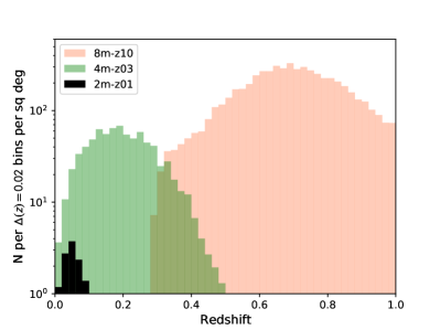
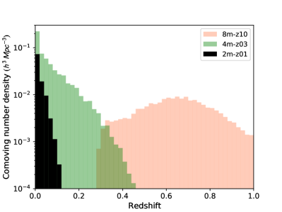
Figure 3: The area density (top) and comoving number density (bottom) of galaxies of the various mock galaxy redshift catalogs used as input for FRB foreground density reconstructions analyzed in this paper. The catalogs will be combined to build up foreground galaxy samples to cover a given FRB redshift. Note that even though the 2m-z01 catalog appears to provide a negligible contribution, its large footprint on the sky enables accurate reconstruction of very low-redshift structures that are otherwise ill-sampled by the narrow high-redshift catalogs.

As seen in the previous section, the IGM component is typically the dominant component of the extragalactic FRB dispersion mesure (see Equation 3 and Figure 1) in both the mean value and scatter. The scatter, $\sigma_{\mathrm{igm}}$, is driven primarily by fluctuations in the underlying large-scale ($\gtrsim$Mpc) cosmic web traversed by the FRB sightlines. We therefore hypothesize that spectroscopic galaxy surveys in the FRB foreground will allow us to significantly reduce $\sigma_{\mathrm{igm}}$ and improve our ability to constrain the parameters governing the CGM and IGM. The H15 lightcone catalog includes synthetic source magnitudes calculated for a variety of photometric filters. Therefore, it is straightforward to select samples of galaxies that simulate various spectroscopic surveys and then study the foreground DM contribution in front of hypothetical FRBs.

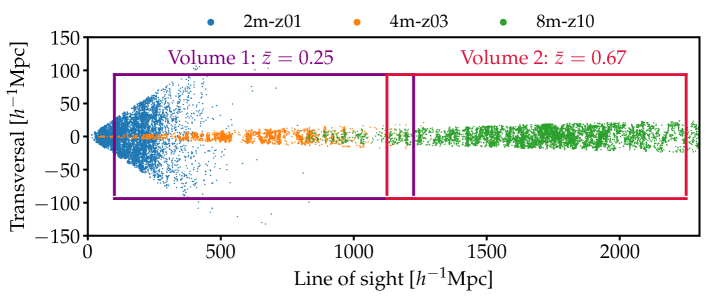
Figure 4: Galaxy positions of the 3 different surveys 2m-z01; 4m-z03; and 8m-z10; used for reconstructions for one mock lightcone. We perform the reconstructions in 2 rectangular boxes consecutively placed along line of sight, dubbed as Volume 1 and Volume 2, leaving a $100\,h^{-1}\rm Mpc$ overlap region. The mean redshifts of the 2 volumes are $\bar{z}_{1}=0.25$ and $\bar{z}_{2}=0.67$, respectively. Note that the aspect ratio is different between the abscissa and ordinate axes in this figure.

We defined several mock spectroscopic catalogs up to $z_{\mathrm{frb}}\leq 0.8$, utilizing multiplexed wide-field spectrographs on a range of telescope sizes. These are described in detail in Appendix A and summarized in Table 1, while Figure 4 provides a visual impression of the various surveys’ coverage for a single lightcone. Depending on the $z_{\mathrm{frb}}$, we will assume a combination of surveys to build up to the desired redshift: for example, for a simulated $z_{\mathrm{frb}}=0.3$ sightline we will assume the availability of the 2m-z01 and 4m-z03 data in the foreground. These mock surveys are coarse-grained in terms of the redshift ranges they cover. Thus, for the mock analysis on a $z_{\mathrm{frb}}=0.6$ FRB there might be many superfluous background galaxies at $z_{\mathrm{gal}}>0.6$ because 8m-z10 observations will cover up to $z=0.8$ (see below). In real observations, the target selection will be fine-tuned individually for the specific $z_{\mathrm{frb}}$ fields that are being targeted in order to maximize the telescope efficiency. Nevertheless, these mock catalogs have been invaluable in helping to design the observational strategy for the FLIMFLAM Survey, which we briefly describe in Section 6.

The area densities and comoving number densities of the different surveys are shown in Figure 3, in which we have averaged all the 24 available H15 lightcones from the Millennium database in order to obtain a smooth redshift distribution — the distributions in the individual 3.1 deg² lightcones are much more uneven due to variations in large-scale structure. While it may appear from Figure 3 as if the 2m-z01 catalog contributes only negligibly to the foreground sampling, the wide-field coverage over hundreds of square degrees is crucial for accurately recovering transverse structures at very low redshifts. Similar data sets to 2m-z01 already exist for much of the extragalactic sky thanks to all-sky spectroscopic surveys such as SDSS (Abazajian et al., 2009) and 6dF (Jones et al., 2009).

For the density reconstructions in the rest of this paper, we used mock catalogs from only 6 of the 24 lightcones released by H15, which were the subsets in which the all-sky catalogs were available — the other 18 lightcones had no data beyond the central 3.1$\,\mathrm{deg}^{2}$ footprints.

3.3 Intervening Galaxy Catalogs

In addition to the wide-field survey redshift data defined above, for each mock FRB sightline we also output an ‘observational’ list of all galaxies within $<10\arcmin$ and $M_{\mathrm{halo}}\geq 3\times 10^{11}\,\mathrm{M}_{\odot}$, listing their redshift, angular separation from the sightline, and estimated halo mass. To mimic a realistic observational scenario, we include all galaxies with the aforementioned criteria whether or not they actually contribute to the sightline $\mathrm{DM}_{\mathrm{halos}}$ given our fiducial parameters. Also, since there are significant uncertainties in estimating galaxy halo masses, we introduce random errors of $\sigma(\log_{10}M_{\mathrm{halo}}/M_{\odot})=0.3$ to the listed halo masses. Separately from the ‘observational’ intervening galaxy list, we also kept track of the true halo masses and $\mathrm{DM}_{\mathrm{halos}}$ contributions for each sightline to calculate the ‘true’ values.

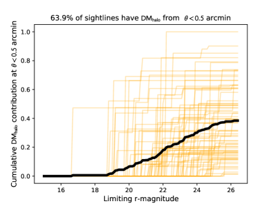
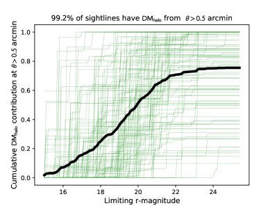
Figure 5: Colored lines indicate cumulative contributions to $\mathrm{DM}_{\mathrm{halos}}$ from mock sightlines extracted from our H15 catalogs, showing the contribution from (top) angular separations of $\theta<0.5\arcmin$, and (bottom) separations of $0.5\arcmin<\theta<5\arcmin$. In each panel, the black curve indicates the average cumulative contribution from all sightlines.

We now comment on the observations required to account for these intervening galaxies, which would be expected to be fainter than the large-scale tracer galaxies described in the previous Section and thus need to be observed with larger telescopes. We analyze an ensemble of 120 random sightlines with $z_{\mathrm{frb}}\leq 0.5$ in Figure 5 to characterize the typical separations and galaxy magnitudes at which intervening halos are likely to contribute to the sightline DM budget. In the top panel of Figure 5, we see that $64\%$ of the mock sightlines have $\mathrm{DM}_{\mathrm{halos}}$ contributions from angular separations of $\theta<0.5\arcmin$, of which on average $\sim 40\%$ of the total $\mathrm{DM}_{\mathrm{halos}}$ contribution is from these small separations. But these closely-intervening galaxies can reach down to relatively faint magnitudes of $r>24$, with about $\sim 10\%$ of the $\mathrm{DM}_{\mathrm{halos}}$ contribution missing from these sightlines if $r>24$ galaxies are unaccounted for.

At slightly larger separations of $0.5\arcmin<\theta<5\arcmin$, we see in the bottom panel of Figure 5 that nearly all (99%) sightlines have contributions from larger angular distances from FRB sightlines. At these larger separations, however, the contributions come from galaxies with typical magnitudes of $r<23$. Indeed, an observational limit of $r<22.5$ would only miss out on a few percent of the overall $\mathrm{DM}_{\mathrm{halos}}$ contribution on these larger separations. We find that on average, there are $\sim 4$ galaxies (up to a maximum of $\sim 12$) with $r<22.5$ that would contribute to each sightline. However, within a radius of $\theta<5\arcmin$ there are likely to be $\sim 100-200$ galaxies at this magnitude limit. Photometric redshifts would therefore be invaluable to pre-select $\sim 20-30$ candidate foreground galaxies that could then be observed with a typical imaging spectrograph on an 8-10m class telescope, to confirm their redshifts.

These results are consistent with the estimates of Ravi (2019) who found that observing galaxies down to $r<24$ would detect $>90\%$ of the $\mathrm{DM}_{\mathrm{halos}}$ contribution, but our findings motivate a tiered observing strategy to target intervening galaxies. First, one desires an integral field unit (IFU) spectrograph observations with 8-10m class telescope (e.g., VLT/MUSE or Keck-II/KCWI) within $\theta\lesssim 0.5\arcmin$ with several-hour integration to reach depths of $r>24$. For larger radii, ($0.5\lesssim\theta\lesssim 5\arcmin$), multiple short pointings ($<1$ hr) with spectrographs on 8-10m class telescopes such as Keck-I/LRIS, VLT/FORS2, or Gemini/GMOS would confirm any intervening galaxies. Note that it is possible for halos to contribute at larger separations of $\theta>5\arcmin$, but these tend to be galaxy group-sized halos or larger ($M\gtrsim 10^{13}\,M_{\odot}$), for which the central galaxies are typically massive and bright enough to be identified through the wide-area surveys described in Section 3.

4 Density Reconstructions

In this section we describe the method used to reconstruct the matter density field given the distribution of the mock galaxy redshifts extracted from H15 as described in the previous section. This reconstructed matter density will be used to place constraints on the possible range of $\mathrm{DM}_{\mathrm{igm}}$ that arises from large-scale diffuse gas in the foreground of individual sightlines.

We will use the most recent version of the ARGO Code (Ata et al., 2015, 2017), which is based on Kitaura & Enßlin (2008); Jasche & Kitaura (2010); Kitaura et al. (2010). First, we describe the reconstruction algorithm ARGO, presenting the necessary formulae and modifications to the algorithm. Then, we describe how the input mock galaxies have been organized and the reconstructions have been performed.

As described in Section 3.2, the different mock catalogs are biased tracers of the same underlying density field. In order to jointly reconstruct the density field from these distinct mock surveys, a multi-survey approach is required. We follow the multi-tracer/multi-survey approach introduced by Ata et al. (2021), which was implemented in the COSMIC BIRTH algorithm (Kitaura et al., 2021). With this approach we can combine separate survey footprints, radial selection functions, galaxy biases and number densities.

4.1 Bayesian Inference Model

The goal of Bayesian inference using Monte Carlo Markov Chains (MCMC) is to draw samples of a posterior probability density $\mathcal{P}(\hbox{\boldmath{$\Theta$}}|\hbox{\boldmath{$d$}})$, representing a set of parameters $\Theta$ given a data vector $d$. The posterior consists of a prior $\pi$ and a likelihood function $\mathcal{L}$

$$\cal P(\hbox{\boldmath{$\Theta$}}|\hbox{\boldmath{$d$}})\propto\pi(\hbox{\boldmath{$\Theta$}})\times\cal L(\hbox{\boldmath{$d$}}|\hbox{\boldmath{$\Theta$}})\,.$$ (8)

In our framework the variable of interest is the linearized matter density $\hbox{\boldmath{$\Theta$}}=\hbox{\boldmath{$\delta$}}_{\rm L}$, that we infer on a rectangular grid with $N_{\rm C}$ cells. The transformation between the physical density contrast $\hbox{\boldmath{$\delta$}}=\hbox{\boldmath{$\varrho$}}/\bar{\hbox{\boldmath{$\varrho$}}}-1$ (matter density $\varrho$ ) and the linearized density $\hbox{\boldmath{$\delta$}}_{\rm L}$ (Coles & Jones, 1991) is

$$\hbox{\boldmath{$\delta$}}_{\rm L}=\log(1+\hbox{\boldmath{$\delta$}})-\hbox{\boldmath{$\mu$}}\,,$$ (9)

where the mean field $\mu$ (Kitaura & Angulo, 2012) ensures $\langle\hbox{\boldmath{$\delta$}}_{\rm L}\rangle=0$. As prior distribution for $\hbox{\boldmath{$\delta$}}_{\rm L}$ we utilize a multivariate Gaussian

$$\pi(\hbox{\boldmath{$\delta$}}_{\rm L})=\frac{1}{\sqrt{(2\pi)^{N_{c}}\det(\rm\bf C_{\rm L})}}\exp\left(-\frac{1}{2}\hbox{\boldmath{$\delta$}}^{\rm T}_{\rm L}\rm\bf C_{\rm L}^{-1}\hbox{\boldmath{$\delta$}}_{\rm L}\right)$$ (10)

where $\rm\bf C_{\rm L}=\langle\hbox{\boldmath{$\delta$}}^{\rm T}_{\rm L}\hbox{\boldmath{$\delta$}}_{\rm L}\rangle$ is the co-variance matrix of the linearized density.

The information content of the data is encoded in the likelihood function that depends on the expected number of galaxies $\lambda$ given the underlying matter field $\delta$ and the observed number of galaxies $\hbox{\boldmath{$N$}}_{\rm G}$. We model the expectation number per cell $i$ as

$$\lambda_{i}=f_{N}w_{i}(1+G_{i}\delta_{i})^{b_{i}}\,,$$ (11)

with the normalization $f_{N}$ ensuring correct number density $\bar{N}$, $w_{i}$ the completeness at cell $i$, and $b_{i}$ the galaxy bias parameter, accounting for the different clustering of galaxies as compared to the total matter. $G_{i}$ is the growth factor ratio between a reference redshift $z_{\rm ref}$ , and an arbitrary redshift $z_{i}$

$$G(z_{\rm ref},z_{i})=D(z_{i})/D(z_{\rm ref})\,,$$ (12)

where

$$D(z_{i})=\frac{H(z_{i})}{H_{0}}\int\limits_{z_{i}}^{\infty}{\rm d}z\frac{1+z}{H^{3}(z)}\bigg{/}\int\limits_{0}^{\infty}{\rm d}z\frac{1+z}{H^{3}(z)}\,.$$ (13)

The factor $G_{i}$ is necessary to account for the redshift dependent clustering evolution if the density field is reconstructed from galaxy positions on a light cone (Ata et al., 2017) when compared to a reference redshift. We will explain this important point in the next section.

We can now write the Poisson likelihood expression for a single survey as

$$\mathcal{L}(\hbox{\boldmath{$N$}}_{{\rm G}}|\hbox{\boldmath{$\lambda$}})=\prod_{i}\frac{\lambda_{i}^{{N}_{{\rm G}i}}{\rm e}^{-\lambda_{i}}}{{N}_{{\rm G}i}!}\,.$$ (14)

As stated above, in this paper we seek a reconstruction given multiple surveys. Thus we formulate a multi-survey likelihood with $k$ surveys as

$$\mathcal{L}^{\rm multi}=\prod_{k}\mathcal{L}^{(k)}(\hbox{\boldmath{$N$}}^{(k)}_{\rm G}|\hbox{\boldmath{$\lambda$}}^{(k)})$$ (15)

This likelihood is then sampled using a Hybrid Monte-Carlo technique (HMC, Duane et al., 1987; Neal, 2011), in which artificial momentum variables are introduced to avoid inefficient random walks in our high-dimensional space of matter density grid cells. Our method is based on that first introduced in Ata et al. (2015), but with a generalization for the multi-survey likelihood. Due to its technical nature, we will describe it in Appendix B.

4.2 Velocity Reconstructions

Another important aspect of the density reconstructions is the iterative correction of so-called redshift space distortions (Kaiser, 1987; Hamilton, 1997), where galaxy positions are displaced along line of sight due to their peculiar motions.

Let us denote the apparent line-of-sight position of a galaxy with $s$, which is the real space position $r$ biased by the radial component of the galaxies’ peculiar motion

$$\hbox{\boldmath{$s$}}=\hbox{\boldmath{$r$}}+\frac{\hbox{\boldmath{$v$}}_{\rm r}}{H(a)\,a}\,,$$ (16)

with

$$\hbox{\boldmath{$v$}}_{\rm r}=(\hbox{\boldmath{$v$}}\cdot\hbox{\boldmath{$r$}})\hbox{\boldmath{$e$}}_{r}\,,$$ (17)

where $\hbox{\boldmath{$e$}}_{r}$ is the radial unit vector.

Solving Equation 16 for $r$ demands the knowledge of $v$, which we can compute from the density contrast using linear perturbation theory as

$$\hbox{\boldmath{$v$}}=-fH(a)\,a\hbox{\boldmath{$\nabla$}}\nabla^{-2}\delta\,,$$ (18)

with $f={\rm d}(\log D)/{\rm d}(\log a)$ being the logarithmic derivative of the growth factor, called growth rate. We solve Equation 16 iteratively in a Gibbs sampling scheme for the real space positions given the inferred density contrast of the previous iteration (see Kitaura et al. 2016).

4.3 Data Preparation & Reconstruction Setup

The mock galaxy positions are given on the sky with right ascension $\alpha$ and declination $\delta$, and observed redshift $z^{\rm obs}$. We map them to comoving Cartesian coordinates as

$$x = d_{\rm com}\cos{\alpha}\cos{\delta}\,,$$

$$y = d_{\rm com}\sin{\alpha}\cos{\delta}\,,$$

$$z = d_{\rm com}\sin{\delta}\,,$$ (19)

where the comoving distance $d_{\rm com}$ is given by

$$d_{\rm com}=\frac{c}{H_{0}}\int\limits_{0}^{z^{\rm obs}}\frac{{\rm d}z}{\sqrt{\Omega_{\rm M}(1+z)^{3}+\Omega_{\Lambda}}}\,.$$ (20)

We organize the reconstructions with two consecutive rectangular volumes (dubbed as Volume 1 and Volume 2), each with $N_{\rm C}=600\times 100\times 100$ cells. With a cell resolution of $d_{\rm Cell}=1.875\,h^{-1}\rm Mpc$ (to match the H15 density field; see Section 2), this leads to a line-of-sight comoving length of $d_{\rm LOS}=1125\,h^{-1}\rm Mpc$, while in transverse dimension it is $d_{\rm Trans}=187.5\,h^{-1}\rm Mpc$. In preliminary tests, we found an unsatisfactory performance for the reconstructions at nearby comoving distances of $d_{\mathrm{com}}\lesssim 100\,h^{-1}\,\mathrm{Mpc}$, which we suspect is caused by the 700$\,\mathrm{deg}^{2}$ footprints of the 2m-z01 samples being insufficiently wide. In a real reconstruction, we expect to be able to use all-sky reconstructions of the Local Universe to cover $d_{\mathrm{com}}\lesssim 100\,h^{-1}\,\mathrm{Mpc}$ (e.g., Erdoǧdu et al., 2006), so we begin our reconstructions at $d_{\mathrm{com}}=100\,h^{-1}\,\mathrm{Mpc}$. Volume 1 thus spans a line of sight range of $L_{\rm LOS}=[100-1225]\,h^{-1}\rm Mpc$, while Volume 2 covers $L_{\rm LOS}=[1125-2250]\,h^{-1}\rm Mpc$. There is an overlap of $100\,h^{-1}\rm Mpc$ between the two volumes for consistency. The coverage of the two reconstruction volumes on one of our mock lightcones is illustrated in Figure 4. We reconstruct the individual volumes at their mean redshifts (see Equation 11), which are $\bar{z}_{1}=0.25$ for Volume 1 and $\bar{z}_{2}=0.67$ for Volume 2.

For Volume 1 we combine the data of the 3 surveys 2m-z01, 4m-z03, and 8m-z10, whereas for Volume 2 we only use 8m-z10 data, as shown in Figure 4.

4.4 Survey Completeness

We model the angular and radial selection function of each mock survey which we then combine to the survey completeness (see Equation 11). In this paper we consider the angular footprint to not have any selection effect, i.e. we assume the angular footprints to be entirely uniform across their entire area as summarized in Table 1. The radial selection function, on the other hand, is more challenging to model. A natural way to model the expected galaxy numbers in radial direction can be done using the Schechter luminosity function (e.g. Erdoǧdu et al. 2004). This is accurate if averaged over the whole sky. In our case, dealing with footprints of $\mathcal{O}(1{\,\rm deg}^{2})$, we are prone to fluctuations in the large-scale structure. Therefore, we average the radial galaxy distribution from the 6 mock lightcones extracted from H15 and calculate the radial selection function from it, see Figure 6.

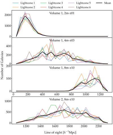
Figure 6: Radial distribution of the different mock surveys. The colors indicate the 6 different lightcones extracted from H15, the black solid line is the mean over the lightcones. The 3 upper panels panels show the contributions of the individual surveys for Volume 1, the bottom panel for Volume 2.

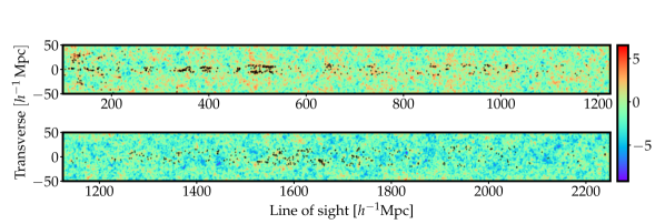
Figure 7: Slice plots of the inferred real space density field $\log(1+\hbox{\boldmath{$\delta$}})$ from ARGO, with “observed” galaxy positions overplotted as black dots. Top panel shows Volume 1, bottom panel Volume 2. As expected, the density field is consistent with the galaxy distribution.

4.5 Galaxy Bias Fits

We seek a single bias fitting function to obtain unbiased density fields for all lightcones extracted from H15. For an initial estimate we use linear bias measurements from completed galaxy surveys, in particular the bias values measured from SDSS (Tegmark et al., 2004) for the low redshift contribution and VIPERS measurements (Di Porto et al., 2016) for the high redshift contribution.

We find that a moderate increase of the galaxy bias with redshift $z$ fits the data sufficiently well, yielding nearly unbiased density fields with respect to the H15 simulations.

$$b(z)=b(z=0.33)+0.22\,z\,$$ (21)

where $b(z=0.33)=1.24$.

However, when we compute the integrated line-of-sight density, we still find a small bias in the resulting values in comparison with the ‘truth’. Due to the time-consuming computational requirements to carry out the reconstructions, it is prohibitive to iterate over different bias models to find a more accurate bias model. Instead, we will correct for the residual bias as a post-processing step which we describe in the following sub-section.

4.6 Reconstruction Results

Examples of the resulting reconstructed real-space matter density fields are shown in Figure 7. The Volume 1 and Volume 2 maps are shown on the top and the bottom panel, respectively. On top of the density slices we plot the inferred real space positions of the galaxies. For each reconstruction, we run the HMC sampler for up to 10,000 iterations. However the posterior samples are found to have correlation lengths of $\sim 100-150$, thus we extract 50 iterations of each density field for analysis with the selected samples separated by at least 150 iterations on the chain. This allows us to not only estimate the integrated line-of-sight dispersion measure, but also its uncertainty.

ARGO reconstructs the real-space matter density field based on input catalogs of galaxy positions and redshifts, but for a given localized FRB with known redshift, we do not have a priori information regarding its real-space position along the line-of-sight. We therefore have to convert the FRB redshift into a line-of-sight comoving distance using the Hubble Law in order to determine its coordinate within the reconstruction box. In other words, we are forced to ignore the line-of-sight peculiar velocity of the FRB host galaxy when computing its integrated line-of-sight dispersion measure. This, however, is typically of order several hundred kilometers per second, corresponding to an error of up to several comoving Mpc along the line-of-sight. For FRBs at cosmological distances, the error from ignoring the peculiar velocity contribution is negligible in comparison with the overall line-of-sight paths of hundreds or thousands of megaparsecs.

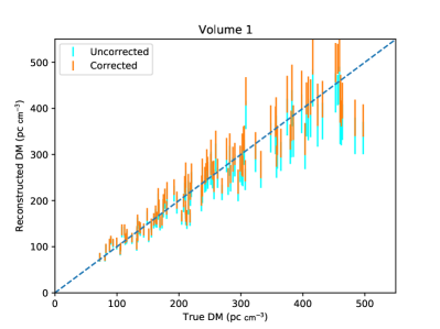
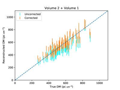
Figure 8: The reconstructed $\mathrm{DM}_{\mathrm{igm}}$ values from the ARGO reconstructions compared with the ‘true’ values in the Millennium simulation, shown in cyan. The top panel shows the results from an ensemble of random sightlines at $0.1<z<0.4$ that are entirely contained within reconstruction Volume 1, while the bottom panel shows the same for $0.45<z<0.8$ sightlines that span both Volumes 2 and 1. The error bars indicate the standard deviation of the reconstructed $\mathrm{DM}_{\mathrm{igm}}$ evaluated over 50 ARGO realizations. The orange bars show the results after correcting the reconstructed $\mathrm{DM}_{\mathrm{igm}}$.

We first smooth the reconstructed density field by $R_{sm}=0.7\,h^{-1}\,\mathrm{Mpc}$ to match the smoothing scale we adopt for the Millennium density field. Next, we calculate $\mathrm{DM_{argo}}$, a version of the discretized line-of-sight integral in Equation 4 in which the smoothed matter density $\delta^{sm}_{m}$ is evaluated on the reconstructed matter density grid from ARGO rather than the ‘true’ Millennium density field as in Equation 4. For the purposes of the analysis in this Section only, we will adopt $f_{\mathrm{igm}}=1$ for simplicity, although it will be considered a free model parameter in our forecasts of Section 5. As noted earlier, our reconstructions skip the first $100\,h^{-1}\,\mathrm{Mpc}$ of the line-of-sight from the observer towards the FRB, so we simply add in a fixed contribution of $\mathrm{DM}_{\mathrm{igm}}(d_{\mathrm{com}}<100\,h^{-1}\,\mathrm{Mpc}\,|\,f_{\mathrm{igm}}=1)=33\,\mathrm{pc}\,\mathrm{cm}^{-3}$ to all the derived $\mathrm{DM}_{\mathrm{igm}}$ values.

Since we know the ‘true’ $\mathrm{DM}_{\mathrm{igm}}$ values for each mock FRB sightline from the H15 Millennium simulations, we can directly assess the accuracy and precision of the $\mathrm{DM_{argo}}$ relative to the true $\mathrm{DM}_{\mathrm{igm}}$. These are shown in Figure 8, where the dispersion measures are evaluated for an ensemble of random ‘FRB’ sightlines at $0.1<z<0.8$ with random angular positions within 12 arcmin of the lightcone field centers. We see that the reconstructed $\mathrm{DM}_{\mathrm{igm}}$ deviate slightly from an exact one-to-one relationship with the true $\mathrm{DM}_{\mathrm{igm}}$, while also having some scatter. We therefore fitted a quadratic offset as a function of the median reconstructed $\mathrm{DM}_{\mathrm{igm}}$ of each sightline to correct this small bias — this was done separately for sightlines contained within Volume 1, and for the combined $\mathrm{DM}_{\mathrm{igm}}$ of Volume 1 and 2 in the case of sightlines that originate in Volume 2. The orange points in Figure 8 show the reconstructed $\mathrm{DM}_{\mathrm{igm}}$ after implementing this correction. In real observations, similar corrections can also be carried out if realistic simulations and mock catalogs that reflect the observational data are available.

Since it is the goal of this paper to carry out Fisher parameter forecasts, it is necessary to check whether the distribution of the reconstructed $\mathrm{DM}_{\mathrm{igm}}$ from the ARGO realizations reflect the uncertainty of the line-of-sight integrated density. To do this, we compute the “pull” distribution, $(\mathrm{DM_{igm,argo}}-\mathrm{DM_{igm,true}})/\sigma_{\mathrm{argo}}$. If the scatter of the ARGO realizations accurately reflects the true error in our estimate of $\mathrm{DM}_{\mathrm{igm}}$, then the pull should be distributed as a Gaussian with a standard deviation of 1. We find the pull distributions of $\mathrm{DM_{igm,argo}}$ to be approximately Gaussian, but with standard deviations of 1.63 and 1.55 for Volume 1 and Volume 1+2, respectively. There is a small skew to the pull distributions, with slightly more outliers at negative values where $\mathrm{DM_{igm,argo}}$ is underestimated relative to $\mathrm{DM_{igm,true}}$. This suggests that the ARGO reconstructions do not currently recover the full amplitude in some of the density peaks. In an actual likelihood analysis on real data, this would need to be corrected to avoid biasing the results. For the purpose of our subsequent Fisher forecast, however, we will treat the pull distribution as Gaussian but broaden the $\mathrm{DM_{igm,argo}}$ distributions of each sightline around its median by the aforementioned factors of 1.63 and 1.35. This rescales the scatter in each sightline as to be more accurate representations of the uncertainty in the $\mathrm{DM}_{\mathrm{igm}}$ measurement from the foreground galaxy redshift measurement.

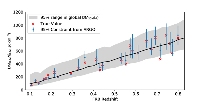
Figure 9: Solid line and gray regions show the mean and central 95% range of the the global $\mathrm{DM}_{\mathrm{igm}}$ distribution within the Millennium simulation as a function of redshift, assuming $f_{\mathrm{igm}}=1$. Red crosses show the $\mathrm{DM}_{\mathrm{igm}}$ toward randomly-selected sightlines within the H15 lightcone catalogs, the blue error bars show the $\mathrm{DM}_{\mathrm{igm}}$ constraint from the ARGO matter density reconstructions of the same catalogs.

We illustrate the efficacy of the ARGO reconstructions in Figure 9, which shows the global $\langle\mathrm{DM}_{\mathrm{igm}}\rangle$ as well as its central 95% distribution (i.e. the range between the 2.5th and 97.5th percentiles of the distribution), as a function of FRB redshift. We also show as crosses the $\mathrm{DM}_{\mathrm{igm}}$ corresponding to some randomly selected sightlines at $0.1<z<0.8$ selected from the lightcones. The error bars show the corresponding constraints on those sightlines obtained by applying ARGO on the foreground spectroscopic surveys described in Section 3.2. The ARGO reconstructions are effective in bracketing the true $\mathrm{DM}_{\mathrm{igm}}$ to within an uncertainty that is $\sim 2-3\times$ smaller than that from cosmic variance. The efficacy does appear to degrade somewhat toward the higher-redshift end ($z\gtrsim 0.7$), with broader errors as well as catastrophic failures where the reconstructed range falls outside the true value. There is ongoing work to improve the performance of ARGO, but in the meantime we will proceed with assuming this performance for our Fisher forecasts.

In all sightlines, the ARGO reconstructions allow us to constrain $\mathrm{DM}_{\mathrm{igm}}$, assuming a fixed $f_{\mathrm{igm}}=1$, with better precision than if the global $\mathrm{DM}_{\mathrm{igm}}$ distribution were to be assumed. Conversely, if $f_{\mathrm{igm}}$ was an unknown parameter, the density fluctuations estimated by ARGO would then be used to fit for the most likely $f_{\mathrm{igm}}$ that leads to the observed $\mathrm{DM}_{\mathrm{igm}}$. This is the scenario that will be adopted in the Fisher forecasts of the following section.

5 Fisher matrix forecast

To predict how accurately we can infer the model parameters from future datasets, we perform a Fisher matrix analysis. Given our four model parameters $p=\{f_{\rm igm},r_{\rm max},f_{\rm hot},\overline{\mathrm{DM}}_{\mathrm{host}}\}$, and the observable $f_{m}\left(p\right)\equiv{\rm DM^{model}_{eg}}$, where the subscript ‘eg’ denotes ‘extragalactic’, and the elements of the Fisher matrix are given by the sum over $m$ FRBs:

$$\mathcal{F}_{i,j}=\sum_{m}\frac{1}{\sigma_{m}^{2}}\frac{\partial f_{m}}{\partial p_{i}}~{}\frac{\partial f_{m}}{\partial p_{j}}.$$ (22)

The model DM, $f_{m}\equiv{\rm DM}^{\mathrm{model}}_{\mathrm{eg,m}}$, is calculated for each individual FRB sightline $m$ in our mock sample:

$${\rm DM}^{\mathrm{model}}_{\mathrm{eg},m}= \langle{\rm DM}_{\mathrm{argo},m}(f_{\mathrm{igm}})\rangle$$

$$+\mathrm{DM}_{\mathrm{halos},m}(r_{\mathrm{max}},f_{\mathrm{hot}})$$

$$+\mathrm{DM_{host}}(1+z_{m})^{-1},$$ (23)

where $\langle{\rm DM}_{\mathrm{argo},m}(f_{\mathrm{igm}})\rangle$ is the median $\mathrm{DM}_{\mathrm{igm}}$ value computed based on the ARGO density reconstruction for sightline $m$, $\mathrm{DM}_{\mathrm{halos},m}(r_{\mathrm{max}},f_{\mathrm{hot}})$ is the $\mathrm{DM}_{\mathrm{halos}}$ computed given the list of intervening halos in sightline $m$ (including 0.3 dex halo mass error), while $z_{m}$ is the redshift of the FRB (Compare with Equation 3). In the model calculation we also make the approximation $\mathrm{DM}_{\mathrm{host}}=\overline{\mathrm{DM}}_{\mathrm{host}}$, i.e. the host contribution is represented by its population mean.

The uncertainty $\sigma_{m}$ on each observable $f_{m}$ is calculated by adding up in quadrature: $\sigma_{\mathrm{MW}}$, the observational uncertainty on the extragalactic dispersion measure after subtraction of the Milky Way component; $\sigma_{\mathrm{igm}}$, uncertainty on the intergalactic contribution from the ARGO reconstructions; $\sigma_{\mathrm{host}}$, the intrinsic scatter in the distribution of rest-frame $\mathrm{DM}_{\mathrm{host}}$; and $\sigma_{\mathrm{halos}}$, the error induced by the uncertain halo mass of the intervening ($\sim$ arcmin-separation) galaxies in the line-of-sight of each mock FRB:

$$\sigma_{m}=\sqrt{\sigma_{\mathrm{MW}}^{2}+\sigma_{\mathrm{igm}}^{2}+\sigma_{\mathrm{halos}}^{2}+\sigma_{\mathrm{host}}^{2}}.$$ (24)

For all FRBs in each mock sample, we assume $\sigma_{\mathrm{MW}}=15\,\mathrm{pc}\,\mathrm{cm}^{-3}$ ensues from subtraction of the Milky Way component as discussed in Section 3.1. The $\sigma_{\mathrm{igm}}$ component is given by the standard deviation of DM_igm,argo along individual sightlines based on the Monte Carlo realizations of the ARGO density reconstructions. This is subsequently corrected to be unbiased and have accurate error properties (Section 4.6). The $\sigma_{\mathrm{halos}}$ component, on the other hand, arises primarily from the halo mass uncertainty which goes into our modified NFW halo gas model (Equations 6 and 7) for intervening galaxies within 10′ of each sightline. We assume that the halo masses can be estimated to within $\pm$0.3 dex, which incorporates uncertainties in estimating galaxy stellar masses and subsequent conversion to halo mass using the stellar mass-halo mass relationship (see, e.g., Wechsler & Tinker, 2018). Therefore, for the $<10\arcmin{}$ intervening galaxy catalog of each sightline, we generated 100 Monte Carlo realizations of the $\mathrm{DM}_{\mathrm{halos}}$ where we randomly drew combinations of different halo masses for the same set of intervening galaxies with $\sigma(\log_{10}M_{\mathrm{halo}}/M_{\odot})=0.3$. The standard deviation of the resulting Monte Carlo realizations of $\mathrm{DM}_{\mathrm{halos}}$ is then adopted as $\sigma_{\mathrm{halos}}$ for that sightline. Finally, we adopt a fixed scatter of $\sigma_{\mathrm{host}}=50\,\mathrm{pc}\,\mathrm{cm}^{-3}$ for the host contribution, which is a guess based on the currently-known sample of localized FRBs (Cordes et al., 2021). In future analyses of real data, we might aim to treat this scatter as a free or unknown parameter.

While the true distributions of the errors above may be non-Gaussian (especially $\sigma_{\rm halo}$), for simplicity we take the standard deviations. To improve the flow of this text, we divert the description on the partial derivatives $\partial f_{m}/\partial p_{i}$ in Equation 22 to the Appendix C. We assume that all cosmological parameters, including $\Omega_{\mathrm{b}}\,h^{2}$, are fixed. The covariance matrix of parameter constraints from a given set of FRBs and their associated foreground data is then given by the inverse of the Fisher matrix, $\mathcal{F}_{i,j}^{-1}$.

Table 2: 68.3% Limits From Fisher Forecast

Parameter	Fiducial Value	$N=30$	$N=96$
$f_{\mathrm{igm}}$	0.8	$\pm 0.11$	$\pm 0.06$
$r_{\mathrm{max}}$/$r_{200}$	1.4	$\pm 0.35$	$\pm 0.15$
$f_{\mathrm{hot}}$	0.75	$\pm 0.15$	$\pm 0.09$
$\mathrm{DM}_{\mathrm{host}}$ ($\mathrm{pc}\,\mathrm{cm}^{-3}$)	100	$\pm 29.21$	$\pm 18.36$

A Fisher forecast yields only the estimated errors from an experiment, i.e. it is not a mock MCMC likelihood analysis which would actually estimate the parameters from a simulated data set. However, many of the partial derivatives in the Fisher matrix (Equation 22), and hence the forecasted errors, do have a dependence on the assumed parameters in the calculation (Appendix C) We therefore adopt the fiducial set of parameters in Table 2, and also impose flat priors such that $0\leq f_{\mathrm{igm}}\leq 1$, $0\leq r_{\mathrm{max}}/r_{200}\leq 5$, $0\leq f_{\mathrm{hot}}\leq 1$, and $0\,\mathrm{pc}\,\mathrm{cm}^{-3}\leq\overline{\mathrm{DM}}_{\mathrm{host}}\leq 1000\,\mathrm{pc}\,\mathrm{cm}^{-3}$.

5.1 Foreground Mapping Constraints

We will make specific forecasts for two hypothetical FRB samples: (i) $N_{\mathrm{frb}}=30$ spanning $0.1<z<0.5$, and (ii) $N_{\mathrm{frb}}=96$ over $0.1<z<0.8$. The $N_{\mathrm{frb}}=30$ sample approximately reflects the goals for the ongoing FLIMFLAM survey as described in Section 6, while foreground data sets covering $N_{\mathrm{frb}}=96$ should be achievable with the advent of 8m-class massively-multiplexed spectrographs.

Early samples of localized FRBs show a roughly uniform redshift distribution (e.g., Heintz et al., 2020). However, the number of known localized FRBs is increasing rapidly and will soon outstrip the number that can be targeted for foreground mapping. At that point, the redshift distribution of FRBs to be targeted for foreground mapping will become a deliberate choice. We therefore choose to adopt a uniform redshift distribution for our mock samples, which is a tradeoff between more expensive observational requirements of higher-redshift FRBs and better constraints on $\overline{\mathrm{DM}}_{\mathrm{host}}$ offered by a wider redshift range. In the longer term ($\gtrsim 2-3$ years) as samples of localized FRBs increase into the hundreds or thousands, the true underlying FRB redshift distribution might turn out not to be uniform with redshift.

From the resulting Fisher matrices, we compute the 68% and 95% error ellipses using standard techniques (usefully summarized in Coe 2009). Figure 10a shows the forecasted confidence intervals for the $N_{\mathrm{frb}}=30$ sample. With foreground spectroscopy from both wide-field surveys (described in Section 3.2) as well as deeper but narrow-field observations of intervening galaxies, we find that the 68.3% confidence constraints are $f_{\mathrm{igm}}=0.80\pm 0.11$, $r_{\mathrm{max}}/r_{200}=1.40\pm 0.35$, $f_{\mathrm{hot}}=0.75\pm 0.15$, and $\overline{\mathrm{DM}}_{\mathrm{host}}=100.0\pm 29.21\;\mathrm{pc}\,\mathrm{cm}^{-3}$.

\begin{overpic}[width=182.1196pt]{n30_fg.pdf} \put(16.0,98.0){{(a) $N_{\mathrm{frb}}=30$ with Foreground Mapping}} \end{overpic}

\begin{overpic}[width=182.1196pt]{n96_fg.pdf} \put(16.0,98.0){{(b) $N_{\mathrm{frb}}=96$ with Foreground Mapping}} \end{overpic}

Figure 10: Fisher matrix forecast on the parameter constraints given by (a) $N_{\mathrm{frb}}=30$ FRB sightlines at $0.1<z<0.5$; and (b) $N_{\mathrm{frb}}=96$ FRB sightlines at $0.1<z<0.8$. The light-blue contours show the $68\%$ confidence intervals, while the dark blue indicates the $95\%$ intervals.

We also experimented with drawing several different random mock samples with the same number of sightlines spanning the same redshift range, and find that there is some heterogeneity in the forecast between the different mock samples with $N_{\mathrm{frb}}=30$. This is caused by the variance in the number of intervening halos in the mock sightlines: ‘clean’ sightlines with few intervening halos tend to be more useful for constraining $f_{\mathrm{igm}}$ and $\mathrm{DM}_{\mathrm{host}}$, whereas sightlines with more intervening galaxies are better for constraining $r_{\mathrm{max}}$ and $f_{\mathrm{hot}}$. This is reflected in the Fisher terms contributed by the individual sightlines (c.f. Equation 22 and Appendix C), where we find that sightlines with more intervening halos have larger values of $\partial\mathrm{DM}_{\mathrm{halos}}/\partial r_{\mathrm{max}}$ and $\partial\mathrm{DM}_{\mathrm{halos}}/\partial f_{\mathrm{hot}}$ than those without. We also note, from experimenting with the redshift range of the sightline distribution, that a broader redshift distribution helps break the degeneracy between $f_{\mathrm{igm}}$ and $\mathrm{DM}_{\mathrm{host}}$ thanks to the $(1+z_{\mathrm{host}})$ denominator associated with $\mathrm{DM}_{\mathrm{host}}$ (Equation 3). As expected, lower redshift FRBs have greater sensitivity toward $\mathrm{DM}_{\mathrm{host}}$. These trends should help guide the choice of FRB sightlines to follow-up with foreground spectroscopy once upcoming surveys start delivering large numbers of localized FRBs.

With $N_{\mathrm{frb}}=96$ sightlines over $0.1<z<0.8$ (Figure 10b), we forecast 68% constraints of $f_{\mathrm{igm}}=0.80\pm 0.06$, $r_{\mathrm{max}}/r_{200}=1.40\pm 0.15$, $f_{\mathrm{hot}}=0.75\pm 0.09$, and $\overline{\mathrm{DM}}_{\mathrm{host}}=100.0\pm 18.36\;\mathrm{pc}\,\mathrm{cm}^{-3}$, i.e. all the IGM and CGM parameters are constrained to within $\sim 10\%$. This shows the high precision that should, in principle, be achievable once the next generation of massive-multiplexed spectroscopic facilities become available.

5.2 Constraints without Foreground Maps

We can also make Fisher forecasts of constraints on the same set of parameters assuming only the redshift and $\mathrm{DM_{eg}}$ from the FRBs, i.e. without any knowledge of the foreground structures or galaxies. In practical terms, this is equivalent to trying to fit a theoretical Macquart relation to the extragalactic dispersion measures and host galaxy redshifts from an observed sample of localized FRBs. The parametric model we need to differentiate for the Fisher matrix then becomes:

$$f_{m}\left(p\right)\equiv{\rm DM}^{\mathrm{model}}_{\mathrm{eg},m}= \langle{\rm DM}_{\mathrm{igm}}(f_{\mathrm{igm}})\rangle(z_{m})$$

$$+\langle\mathrm{DM}_{\mathrm{halos}}(r_{\mathrm{max}},f_{\mathrm{hot}})\rangle(z_{m})$$

$$+\overline{\mathrm{DM}}_{\mathrm{host}}(1+z_{m})^{-1}.$$ (25)

Instead of the per-sightline model calculations that are feasible with foreground spectroscopic data, we are now forced to use the global $\langle\mathrm{DM}_{\mathrm{igm}}\rangle(z)$ and $\langle\mathrm{DM}_{\mathrm{halos}}\rangle(z)$ (i.e. Figure 1a), evaluated at the redshift of each FRB (see Appendix C for the partial derivatives). Similarly, for the $\sigma_{m}$ calculation (Equation 24) we insert the global scatter for $\sigma_{\mathrm{igm}}$ and $\sigma_{\mathrm{halos}}$ (see Figure 1b) instead of bespoke calculations based on the foreground data from each sightline. The forecasted parameters for the same mock sample of $N_{\mathrm{frb}}=96$ — but without any foreground information — is shown in Figure 11. The constraining power clearly is much weakened in the absence of foreground data, with confidence intervals $\sim 2-5\times$ broader in all the parameters. In addition, the degeneracy between $r_{\mathrm{max}}$ and $\mathrm{DM}_{\mathrm{host}}$ appears to have increased when foreground data is unavailable.

How much information does the foreground data bring to cosmic baryon census, in addition to that offered by the localized FRBs and their measured $\mathrm{DM_{eg}}$ values alone? We can attempt to quantify this by rescaling the elements of the no-foreground Fisher matrix (which yields the forecast in Figure 11) until the resulting constraints are roughly the same as if foreground data is available (Figure 10b) for the same sightlines. This is equivalent to increasing the number of sightlines available for analysis by that factor. We find that to approximately match the constraints of $N_{\mathrm{frb}}=96$ in Figure 10b, we had to rescale the no-foreground Fisher matrix elements by $\sim 25\times$. In other words, the foreground data improves the Fisher information content such that every localized sightline that has a foreground map is equivalent to $\sim 25$ localized FRBs where only their redshift and total DM is known. Without foreground data, samples of $N_{\mathrm{frb}}\gtrsim 2000$ localized FRBs with known redshifts would be required to achieve similar constraints as $N_{\mathrm{frb}}\sim 100$ localized FRBs with foreground data. This is qualitatively consistent with the recent analysis of Batten et al. (2021a), who found that $\sim 10^{3}$ localized FRBs are needed to distinguish between their no-feedback simulations and those with feedback (i.e. in effect, detect the existence of the CGM); whereas $\sim 10^{4}$ localized FRBs would be needed to distinguish between galaxy feedback models which lead to different CGM properties.

\begin{overpic}[width=182.1196pt]{figures/n96_no_fg.pdf} \put(18.0,98.0){{$N_{\mathrm{frb}}=96$ without Foreground Data}} \end{overpic}

Figure 11: Parameter forecast in the case of $N_{\mathrm{frb}}=96$ localized FRB sightlines, for which no foreground data is available. The constraints are clearly considerably weakened from the lack of foreground data (c.f. Figure 10).

5.3 Comparison with Previous Forecasts

Our forecasts are, on the surface, more pessimistic than previous efforts in the literature. Walters et al. (2019), for example, carried out a MCMC likelihood forecast and argued that $N_{\mathrm{frb}}=100$ localized FRB sightlines without any foreground data should be able to constrain total diffuse baryon fraction (i.e. combined IGM and CGM components) $f_{d}$ to within a few percent at 95% confidence level. Meanwhile, Ravi (2019) assumed the spectroscopic observations would be available for intervening galaxies within several arcminutes of each FRB sightline, and argued that $f_{\mathrm{igm}}$ could be constrained to within $\sim 2-5\%$ at 95% confidence with $N_{\mathrm{frb}}=100$. Both of these previous forecasts were built on analytic models. In particular, they both assumed that the uncertainty in the DM contribution of the cosmic web or diffuse IGM is given by a standard deviation of $\sigma_{\mathrm{igm}}=10\,\mathrm{pc}\,\mathrm{cm}^{-3}$. This value, which was taken from analytic estimates by Shull & Danforth (2018), is a significant underestimate of the $\sigma_{\mathrm{igm}}$ compared with simulation results by a factor of $>5$ (see Figure 1, and see also Batten et al. 2021b). Such a small $\sigma_{\mathrm{igm}}$ is indeed even tighter than our ARGO constraints on individual line-of-sight dispersion measures as seen in Figure 9. Apart from this discrepancy, it is hard to make direct comparison with the earlier works since we have also adopted simultaneous constraints on galaxy halo parameters as well as the host DM contribution. Both Walters et al. (2019) and Ravi (2019) assumed a fixed $\mathrm{DM}_{\mathrm{host}}$ with some uncertainty, while Ravi (2019) assumed fixed halo parameters for the intervening foreground galaxies. We therefore argue that our forecasts are a more realistic determination of the precision that can be achieved with upcoming FRB samples.

6 FRB Foreground Mapping on the AAT

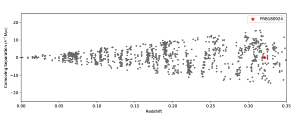
Figure 12: Positions of galaxies in the foreground of FRB180924, based on a preliminary reduction of our 2dF-AAOmega data. The grey dots show comoving coordinates of galaxies within a $10\,h^{-1}\,\mathrm{Mpc}$ slice along the plane of real ascension, with the position of the FRB host galaxy indicated by the red star.

As part of an effort to actualize the technique of FRB foreground mapping introduced in this paper, we have recently commenced the FRB Line-of-sight Ionization Measurement From Lightcone AAOmega Mapping (FLIMFLAM) Survey. This is a nominally $\sim$40-night observational survey on the 2dF-AAOmega fiber spectrograph on the 3.9m Anglo-Australian Telescope (AAT; Lewis et al. 2002, Sharp et al. 2006) to map out the large-scale cosmic web in front of FRBs. Due to the preliminary stage of our data collection and analysis, we simply give a brief introduction to the project in this section and defer a more detailed description to future papers.

The nominal goal of FLIMFLAM is to spectroscopically map the foreground of $N_{\mathrm{frb}}\sim 30$ localized FRBs over the redshift range $0.1<z<0.5$ in order to achieve $\sim 15-20\%$ constraints on $f_{\mathrm{igm}}$ as forecasted in the previous section. The lower redshift limit is because $z\lesssim 0.1$ foreground galaxies are typically covered by publicly-available redshift surveys like 2MASS, 6dF, and SDSS that cover large fractions of the extragalactic sky, while the upper limit of $z<0.5$ was deemed the highest practical redshift for which we can obtain reasonable samples of foreground galaxies within $\sim$ 2-3 nights of observing time per field. Given the location of the AAT in Siding Spring, Australia, it is well-situated to follow up the increasing numbers of localized Southern Hemisphere FRBs being discovered predominately by the Commensal Real-Time ASKAP Fast Transient (CRAFT, Shannon et al., 2018) survey located also in Australia, with subsequent host galaxy follow-up being conducted by the F⁴ collaboration. This collaboration is, at the time of writing, the largest single source of localized FRBs. We are in close collaboration with both CRAFT and F⁴ teams which allows rapid access to FRB coordinates and redshifts as they are identified and localized, although we will also target FRBs from other sources that have publicly available localizations and redshifts.

For each FRB field, we will typically observe multiple plate configurations over a single pointing of 2dF-AAOmega’s $3.1\;\mathrm{deg}^{2}$ field-of-view. Our target selection for a fiducial $z=0.3$ FRB field is similar to the “4m-z03” mock sample described in Section 3.2, namely a nominally complete targeting of $r_{\mathrm{AB}}<19.8$ galaxies. Given the $\sim 350$ science fibers, it therefore takes seven repeated visits on 2dF-AAOmega to target all $\sim 2400$ galaxies with this selection. Assuming 40 minutes of on-sky integration time and 20 minutes of overhead time (detector readout, calibration exposures etc), it takes 7 hours of AAT time to observe the foreground field for a $z=0.3$ FRB. For FRBs at different redshifts, we adjust the $r$-magnitude limit of the foreground galaxies: for FRBs at $z<0.2$, we will adopt $r_{\mathrm{AB}}<19.2$, while conversely at $z>0.4$ we will target $r_{\mathrm{AB}}<20.6$ galaxies. This leads to roughly 1500 and 4800 foreground galaxies for the $z<0.2$ and $z>0.4$ fields, respectively, while for the fainter galaxies we have to increase on-sky exposures up to 90 minutes per galaxy. We use the 580V grating on the blue camera and 385R grating on the red in conjunction with the $5700\,\mathrm{\AA}$ dichroic in order to achieve a spectral resolution of $R\equiv\lambda/\Delta\lambda\sim 1100-1500$ over $3750\,\mathrm{\AA}<\lambda<8850\,\mathrm{\AA}$ — a well-established setup for measuring galaxy redshifts on 2dF-AAOmega.

Assuming a roughly uniform redshift distribution of FRBs within $0.1<z<0.5$, this leads to an average requirement of $\sim 1$ night of on-sky observations per FRB. For $N_{\mathrm{frb}}=30$, this leads to a total requirement of $\sim$40 nights if we add on a 33% weather overhead. We commenced pilot observations in October 2020 and so far have had a total of 17.5 nights allocated through semester 2021B. We show some preliminary data on the foreground field of FRB180924 in Figure 12, where we had first transformed the celestial coordinates and redshifts of the foreground galaxies into comoving Cartesian coordinates using the transformations described by Equations 4.3 and 20. The foreground galaxies clearly trace out the cosmic web of large-scale structure even by eye, and should allow us to confirm whether the low DM values of FRB180924 is indeed due to an underdense foreground (Simha et al., 2021).

FLIMFLAM observations are not the only piece of the puzzle for successfully carrying out FRB foreground mapping. For FRB fields that do not have pre-existing imaging coverage from publicly-available surveys such as the DES or Pan-STARRS, we are using the Dark Energy Camera to obtain pre-imaging on our targeted FRB fields. In addition, we are also pursuing a coordinated campaign to observe the FLIMFLAM fields with 8-10m class telescopes in order to obtain spectra of intervening galaxies at $\sim 5\arcmin$ separations of the sightline down to limiting magnitudes of $\sim 24$.

7 Conclusion

In this paper, we analyzed the ability of spectroscopic foreground data, including wide-field galaxy surveys, to improve on the ability of localized fast radio bursts to constrain the cosmic baryon distribution. Using semi-analytic models for the cosmic dispersion measure that are consistent with those from hydrodynamical simulations, we created mock data samples of both FRB dispersion measures and foreground galaxy catalogs,. We then applied ARGO, a state-of-the-art Bayesian density reconstruction algorithm, on the foreground galaxy catalogs to reconstruct the matter density field. This allows us to constrain the line-of-sight matter density integrand of $\mathrm{DM}_{\mathrm{igm}}$ to $\sim 2-3\times$ better precision than allowed by cosmic variance. In conjunction with spectroscopic data on the intervening galaxy halos within $<10\arcmin$, we make Fisher forecast of the simultaneous constraints on parameters governing the IGM and CGM baryons that could be attainable with upcoming samples of localized FRBs. We find that the foreground data enhances the constraining power on our parameters of interest by a factor of $\sim 25\times$ over samples of localized FRBs without foreground data.

Based on our analysis, we are now conducting various observations to gather foreground observations on $\sim 30$ FRBs sightlines. This observational campaign includes FLIMFLAM, a spectroscopic galaxy redshift survey on the AAT designed to map out the foreground cosmic web in these fields. In addition to the observations, we are also actively building on the methods presented in this paper to create a parameter estimation framework based on Bayesian Markov Chain Monte Carlo (MCMC).

In this paper, we have assumed a $\mathrm{DM}_{\mathrm{host}}$ distribution in the range of $100\,\mathrm{pc}\,\mathrm{cm}^{-3}\lesssim\mathrm{DM}_{\mathrm{host}}\lesssim 300\,\mathrm{pc}\,\mathrm{cm}^{-3}$ in the FRB restframe. However, recent results (Niu et al., 2021) hint at the existence of FRBs with much larger host dispersions ($\mathrm{DM}_{\mathrm{host}}\sim 1000\,\mathrm{pc}\,\mathrm{cm}^{-3}$). FRBs with such large $\mathrm{DM}_{\mathrm{host}}$ could potentially contaminate a FRB sample intended for cosmic baryon analysis, leading to biased parameter constraints. There are several possible ways to ensure that only ‘normal’ FRBs with $\mathrm{DM}_{\mathrm{host}}\sim 200\,\mathrm{pc}\,\mathrm{cm}^{-3}$ are included in a cosmic baryon analysis sample. Methods are emerging to model the FRB host contribution, including estimating the host galaxy DM using resolved observations of FRB locations within their host galaxy (e.g., Chittidi et al., 2020; Mannings et al., 2020; Marcote et al., 2020), or by modelling the Balmer line in the host galaxy spectra (e.g., Tendulkar et al., 2017; Bassa et al., 2017; Niu et al., 2021). Evidence is also beginning to emerge that FRBs with unusually high $\mathrm{DM}_{\mathrm{host}}$ also exhibit various properties that differ from ‘normal’ FRBs, such as repeatability, scattering, Faraday rotation measure, and others (R. Shannon, private communication). We therefore expect our framework to study cosmic baryons to be largely unaffected by the existence of high-$\mathrm{DM}_{\mathrm{host}}$ sources.

Recently, Cordes et al. (2021) published an analysis of 14 localized FRBs in which they combined the observed DM together with scattering times to assess the reported host redshifts. They found that adopting a value of $f_{\mathrm{igm}}=0.85\pm 0.05$ lead to the most optimal redshift constraints, leading them to question the host galaxy associations of two FRBs in the sample. This suggests that, for a sample of FRBs with high-confidence host galaxy associations and redshifts (e.g. using the PATH method; Aggarwal et al. 2021), the scattering time of the FRB is a valuable piece of information that can in principle be combined with foreground spectroscopic data to further tighten constraints beyond those forecasted in this paper.

By the middle of the 2020s, the number of localized FRBs will almost certainly increase into the hundreds, especially once Northern Hemisphere radio arrays such as the Deep Synoptic Array (DSA; Kocz et al., 2019) and CHIME Fast Radio Burst Project (CHIME/FRB Collaboration et al., 2018) acquire the capability to localize FRBs. By then, next-generation massively-multiplexed 4m-class spectroscopic facilities such as DESI (Levi et al., 2013) and WEAVE (Dalton et al., 2012) will map large numbers of FRB foregrounds more efficiently than FLIMFLAM at $z<0.5$, while 8m-class spectroscopic facilities such as Subaru PFS (Sugai et al., 2015) and MOONS (Cirasuolo et al., 2014) will also be available to push FRB foreground mapping to higher redshifts. It will then become feasible to comprehensively constrain the cosmic partition of baryons in diffuse gas, and indeed potentially push towards the epoch of Helium-II reionization ($z\sim 3$) with sufficient allocations of telescope time.

Appendix A Detailed Description of Wide-Field Spectroscopic Surveys

In this Appendix, we explain how we designed the mock wide-field foreground spectroscopic surveys defined in Section 3.2. Note that the galaxy photometry and number counts selected from the Henriques et al. (2015) catalog are somewhat dependent on the assumptions of the simulation and semi-analytic model, and might depart from reality especially at higher redshifts. Thus, while we make ad hoc photometric cuts on these mock catalogs to select the desired number density of galaxies at specific redshift ranges, we expect real observations to use more realistic and refined selection criteria to achieve comparable galaxy number densities. The observing requirements we outline in here should, however, be approximately correct in terms of exposure times as a function of magnitude, since they are based on the known performance of existing facilities.

       2m-z01

For much of the extra-galactic sky, there already exists good coverage of galaxy redshifts out to $z\lesssim 0.1$ that were obtained by 1-2m diameter class survey telescopes. In the Northern Hemisphere, the Sloan Digital Sky Survey (SDSS) Main Galaxy Survey (Abazajian et al., 2009; Blanton et al., 2005) on the 2.5m SDSS Telescope (Gunn et al., 2006) has provided good spectroscopic coverage out to $z\lesssim 0.2$. Meanwhile, the 6dF Galaxy Redshift Survey (6dFGRS, Jones et al., 2009) has covered the Southern Hemisphere with the 1m UK Schmidt Telescope, albeit with slightly lower redshfit ($z\lesssim 0.1$). The wide-field coverage of these surveys helps mitigate the boundary effects caused by limited field-of-view in more targeted surveys with larger telescopes. For example, at $z=0.03$, two degrees on the sky corresponds to only 3 Mpc in the transverse dimension, which makes it difficult to accurately reconstruct structures or indeed sample any galaxies from said structures. We note that while Simha et al. (2020) used SDSS data to reconstruct the foreground structures in front of the $z_{\mathrm{frb}}=0.1178$ FRB190608, this was in the relatively narrow Stripe 82 equatorial region and thus suffers from narrow-angle effects at the lowest redshifts ($z\lesssim 0.05$) — they did not use 6dFGRS data which has wide-area coverage in the same region. This narrow-angle aliasing introduces additional uncertainty to the density reconstructions unless wide-field data is incorporated at low redshifts. We therefore use the ‘all-sky’ H15 lightcones from the Millennium database to generate this catalog, with an ad hoc magnitude selection of $r<16.4$ to define a sample peaked at $z_{\mathrm{gal}}\sim 0.05$, similar to 6dFGRS (Jones et al., 2009). This yields an area density of $12\,\mathrm{deg}^{-2}$, with which we generated a catalog spanning 700 sq deg in order to ensure wide-area coverage in the Local Universe.

      4m-z03

Out to $z\sim 0.35$, it is straightforward to obtain large numbers of redshifts using both existing and upcoming 4m-class spectroscopic facilities over at least several square degrees. For example, the GAMA survey (Driver et al., 2011; Liske et al., 2015) has covered 286 sq deg at this redshift range using the AAOmega spectrograph on the 4m Anglo-Australian Telescope — conveniently, the individual H15 lightcones have the same field-of-view (3.1 sq deg) as AAOmega. We adopt the same magnitude cut as GAMA ($r<19.8$) to generate this mock sample, which yields $770\,\mathrm{deg}^{-2}$ of galaxies — with the $\sim 320$ useable fibers on AAOmega (Liske et al., 2015), this would require about 4-5hrs on-sky per FRB field assuming 30-45min exposure times per object. In the near future, the Bright Galaxy Survey carried out with the 4m Dark Energy Spectroscopic Instrument (DESI, Levi et al., 2013; DESI Collaboration et al., 2016) will cover the entire Northern Hemisphere to similar depth, redshift range, and number density as GAMA, making it a powerful complement for future Northern radio experiments capable of FRB localization.

      8m-z10

At higher redshifts ($z\gtrsim 0.4$), 8m-class telescopes are required to achieve the necessary depths to obtain redshifts of typical galaxies, while simultaneously having sufficient multiplexing and field-of-view to observe large numbers of galaxies, thus the Prime Focus Spectrograph (PFS, Sugai et al. 2015) on the 8.2m Subaru Telescope is the ideal instrument for this regime. Since the Subaru Telescope is in the Northern Hemisphere, we assume that both SDSS and DESI Bright Galaxy Survey data will be available to cover lower redshifts, and define a target sample to cover $0.3\lesssim z\lesssim 1$. We adopt a photometric color-color selection inspired by that of the VIPERS survey (Guzzo et al., 2014):

$$(r-i)>2\> \mathrm{or} \>(r-i)>0.5\,(u-g),$$

$$i < 22.75,$$

$$r > 22.8,$$

where we have made ad hoc modifications to get the desired redshift range within the H15 lightcones. Also, the transverse comoving distance increases with redshift fixed angular separation (e.g. at $z=0.7$, one angular degree on the sky subtends 44 cMpc in the transverse dimension), it is possible to decrease the assumed field-of-view at reduced loss to our ability to recover transverse structures. We therefore reduce the footprint of the 8m-z10 mock catalog from 3.1 sq deg in the lower-redshift samples, in order to match the 1.25 sq deg of Subaru PFS. These selections lead to a target density of $5700\;\mathrm{deg}^{-2}$, implying that Subaru PFS should be able to observe each $z_{\mathrm{frb}}\sim 1$ field within approximately 3hrs, assuming 45min exposure times per galaxy like VIPERS which was also a 8.2m-class instrument. For FRBs at intermediate redshifts such as $z\sim 0.5$, it is possible to define target selections to cover those redshifts at a depth that is accessible to 4m-class facilities like AAT/2dF-AAOmega, albeit with deeper integrations than defined in 4m-z03 above. However, due to the computational expense of running the density reconstructions, in the mock analysis for this paper we will use the reconstruction volumes using 8m-z10 catalog even for sightlines at $z\sim 0.5$.

Appendix B Hamiltonian Monte-Carlo for Multi-Surveys

In this Appendix, we will generalize the Hamiltonian Monte-Carlo formalism from Ata et al. (2015) to sample the multi-survey likelihood defined in Equation 14.

Firstly, we define the Hamiltonian $\mathcal{H}(\hbox{\boldmath{$q$}},\hbox{\boldmath{$p$}})$, a function of the canonical coordinates of position $q$ and momentum $p$. Introducing the potential energy $\mathcal{U}(\hbox{\boldmath{$q$}})$ and the kinetic energy $\mathcal{K}(\hbox{\boldmath{$p$}})$, we write

$$\mathcal{H}(\hbox{\boldmath{$q$}},\hbox{\boldmath{$p$}})=\mathcal{U}(\hbox{\boldmath{$q$}})+\mathcal{K}(\hbox{\boldmath{$p$}})\,,$$ (B1)

with the kinetic term

$$\mathcal{K}(\hbox{\boldmath{$p$}})=\frac{1}{2}\hbox{\boldmath{$p$}}^{\rm T}\rm\bf M^{-1}\hbox{\boldmath{$p$}}\,,$$ (B2)

where $\rm\bf M$ is the positive definite mass matrix, representing the co-variance of the momenta $\rm\bf M=\langle\hbox{\boldmath{$p$}}^{\rm T}\hbox{\boldmath{$p$}}\rangle$.

The posterior probability density then written as

$$\mathcal{P}(\hbox{\boldmath{$q$}},\hbox{\boldmath{$p$}})=\frac{1}{Z}\,{\rm e}^{-\mathcal{H}(\hbox{\boldmath{$q$}},\hbox{\boldmath{$p$}})}\,,$$ (B3)

where $Z$ acts as normalization of the posterior. Plugging in Equation B1 into Equation B3, we get

$$\mathcal{P}(\hbox{\boldmath{$q$}},\hbox{\boldmath{$p$}})=\frac{1}{Z}\,\mathcal{P}(\hbox{\boldmath{$q$}})\mathcal{P}(\hbox{\boldmath{$p$}})=\frac{1}{Z}\,{\rm e}^{-\mathcal{U}(\hbox{\boldmath{$q$}})}\,{\rm e}^{-\mathcal{K}(\hbox{\boldmath{$p$}})}\,.$$ (B4)

We can see that the posterior now factorized into two separated probabilities depending solely on the potential energy: $\mathcal{P}(\hbox{\boldmath{$q$}})$, and the kinetic energy: $\mathcal{P}(\hbox{\boldmath{$p$}})$. Considering only the potential term of Equation B4 , we get:

$$\mathcal{U}(\hbox{\boldmath{$q$}})=-\ln\mathcal{P}(\hbox{\boldmath{$q$}})\,,$$ (B5)

and finally for the kinetic term $K(\hbox{\boldmath{$p$}})$:

$$\mathcal{P}(\hbox{\boldmath{$p$}})\propto{\rm e}^{-\mathcal{K}}={\rm e}^{-\frac{1}{2}\hbox{\boldmath{$p$}}^{\rm T}\rm\bf M^{-1}\hbox{\boldmath{$p$}}}\,,$$ (B6)

which resembles a multivariate Gaussian distribution.

Now, in HMC the spatial positions are identified as parameters that we want to sample $\hbox{\boldmath{$q$}}=\hbox{\boldmath{$\delta$}}_{\rm L}$, in our case the linearized density per cell. In contrast, the momentum variables, $p$, are artificially introduced in each sampling step so that the HMC algorithm avoids ineffective random walks to move through the phase space. We use the Hamiltonian equations of motion to evolve the system in (pseudo-)time $t$. The partial derivatives of the Hamiltonian determine how $q$ and $p$ change with time, $t$, according to Hamilton’s equations of motion

$$\frac{\rm d\hbox{\boldmath{$q$}}}{\rm dt} = \frac{\partial{\mathcal{H}}(\hbox{\boldmath{$q$}},\hbox{\boldmath{$p$}})}{\partial\hbox{\boldmath{$p$}}}=\rm\bf M^{-1}\hbox{\boldmath{$p$}}\,,$$ (B7)

$$\frac{\rm d\hbox{\boldmath{$p$}}}{\rm dt} = -\frac{\partial{\mathcal{H}}(\hbox{\boldmath{$q$}},\hbox{\boldmath{$p$}})}{\partial\hbox{\boldmath{$q$}}}=-\frac{\partial\mathcal{U}(\hbox{\boldmath{$q$}})}{\partial\hbox{\boldmath{$q$}}}\,.$$ (B8)

We use the leap-frog discretization scheme, which preserves phase space volume and is time reversible. For a single iteration we calculate the positions and momenta from $t$ to $t+\epsilon$ as follows

$$\hbox{\boldmath{$p$}}\left(t+\frac{\epsilon}{2}\right) = \hbox{\boldmath{$p$}}(t)-\frac{\epsilon}{2}\frac{\partial\mathcal{U}}{\partial\hbox{\boldmath{$q$}}}(\hbox{\boldmath{$q$}}(t))$$ (B9)

$$\hbox{\boldmath{$q$}}(t+\epsilon) = \hbox{\boldmath{$q$}}(t)+\epsilon\,\rm\bf M^{-1}\,\hbox{\boldmath{$p$}}\left(t+\frac{\epsilon}{2}\right)$$ (B10)

$$\hbox{\boldmath{$p$}}(t+\epsilon) = \hbox{\boldmath{$p$}}\left(t+\frac{\epsilon}{2}\right)-\frac{\epsilon}{2}\frac{\partial\mathcal{U}}{\partial\hbox{\boldmath{$q$}}}(\hbox{\boldmath{$q$}}(t+\epsilon))\,.$$ (B11)

The leap-frog scheme introduces numerical errors of order $\mathcal{O}(\epsilon^{3})$ so that one has to introduce a Metropolis-Hastings rejection step. The new state obtained after $N_{\epsilon}$ steps forward with step size $\epsilon$ will be accepted with a probability of

$${\cal P}_{\rm acceptance}=\min\left[1,{\rm e}^{-\Delta\mathcal{H}(\hbox{\boldmath{$q$}},\hbox{\boldmath{$p$}})}\right]\,,$$ (B12)

where $\Delta\mathcal{H}(\hbox{\boldmath{$q$}},\hbox{\boldmath{$p$}})=\mathcal{H}(\hbox{\boldmath{$q$}}^{\prime},\hbox{\boldmath{$p$}}^{\prime})-\mathcal{H}(\hbox{\boldmath{$q$}},\hbox{\boldmath{$p$}})$ is the difference in the Hamiltonian between the old $(\hbox{\boldmath{$q$}},\hbox{\boldmath{$p$}})$ and new $(\hbox{\boldmath{$q$}}^{\prime},\hbox{\boldmath{$p$}}^{\prime})$ state.

According to Equations B5 and B7 we need the negative natural logarithm of the posterior of Equation 8 and its gradient with respect to the linearized density $\hbox{\boldmath{$\delta$}}_{\rm L}$:

$$-\ln\mathcal{P}=-\ln\pi-\ln\mathcal{L}^{\rm multi}\,,$$ (B13)

where

$$-\ln\mathcal{L}^{\rm multi}=\sum_{k}-\ln\mathcal{L}^{(k)}\,.$$ (B14)

Thus, we write for the prior of Equation 10

$$-\ln\pi(\delta_{\rm L})=\frac{1}{2}\hbox{\boldmath{$\delta$}}^{\rm T}_{\rm L}\rm\bf C_{\rm L}^{-1}\hbox{\boldmath{$\delta$}}_{\rm L}+\rm const\,,$$ (B15)

where $\rm const$ does not depend on $\hbox{\boldmath{$\delta$}}_{\rm L}$.

For the likelihood defined in Equation 14, we get

$$-\ln\mathcal{L}^{\rm multi}(\hbox{\boldmath{$N$}}_{{\rm G}}|\hbox{\boldmath{$\lambda$}})=\sum_{k}\sum_{i}\lambda^{(k)}_{i}-{N}^{(k)}_{{\rm G}i}\ln\lambda^{(k)}_{i}+\rm const\,,$$ (B16)

where $\rm const$ is a constant that does not depend on $\hbox{\boldmath{$\delta$}}_{\rm L}$. After defining the logarithms, we write the gradients as

$$-\frac{\partial\ln\pi}{\partial\hbox{\boldmath{$\delta$}}_{\rm L}}=\rm\bf C_{\rm L}^{-1}\hbox{\boldmath{$\delta$}}_{\rm L}\,,$$ (B17)

and for the individual $k$ survey likelihoods at cell $i$

$$-\frac{\partial\ln\mathcal{L}^{(k)}}{\partial\delta_{{\rm L}i}}=b\left(\lambda^{(k)}_{i}-{N}^{(k)}_{{\rm G}i}\right)\,.$$ (B18)

Appendix C Fisher Matrix Partial Derivatives and Priors

In this Appendix, we derive the partial derivatives of the our model relative to the free parameters $\{p_{1},p_{2},p_{3},p_{4}\}\equiv\{f_{\rm igm},{\rm DM_{host}},r_{\rm max},f_{\rm hot}\}$, $\partial f_{m}/\partial p_{i}$, which we use in the Fisher matrix calculations (see Equation 22) to forecast the precision on the parameter estimate.

C.1 Case of available foreground data

First, we calculate the partial derivatives in our default case, where we have information on the foreground matter distribution and intervening galaxies. In this case, the observable $f_{m}\left(p\right)$ for each individual FRB in the sample is given by the model of the total extragalactic DM component

$$f_{m}\left(p\right)={\rm DM}_{\rm igm}\left(f_{\rm igm}\right)+{\rm DM}_{\rm halo}\left(r_{\rm max},f_{\rm hot}\right)+{\rm DM_{host}}\times\left(1+z\right)^{-1},$$ (C1)

For the first parameter $f_{\rm igm}$, we find

$$\frac{\partial f_{m}}{\partial p_{1}}=\frac{\partial~{}{\rm DM}_{\rm igm}\left(f_{\rm igm}\right)}{\partial f_{\rm igm}}=\frac{\langle{\rm DM_{argo}}\rangle}{f_{\mathrm{igm}}}$$ (C2)

where $\langle{\rm DM_{argo}}\rangle$ is the mean of ${\rm DM_{igm}}$ values calculated from the $N=50$ ARGO reconstructed density realizations. Since $\langle\mathrm{DM_{argo}}\rangle$ is linear in $f_{\mathrm{igm}}$, taking its derivative is equivalent to setting $f_{\rm igm}=1$.

Next, the partial derivative for ${\rm DM_{host}}$ is given by

$$\frac{\partial f_{m}}{\partial p_{2}}=\frac{\partial\left({\rm DM_{host}}\times\left(1+z_{m}\right)^{-1}\right)}{\partial~{}{\rm DM_{host}}}=\left(1+z_{m}\right)^{-1},$$ (C3)

where $z_{m}$ is the redshift of the FRB.

In order to find partial derivative for $r_{\rm max}$,

$$\frac{\partial f_{m}}{\partial p_{3}}=\frac{\partial{\rm DM_{\rm halos}}\left(r_{\rm max},f_{\rm hot}\right)}{\partial r_{\rm max}},$$ (C4)

where we numerically differentiate the modified NFW profiles (see Section 3.1) of each mock foreground galaxy in the line-of-sight of the FRB in question with respect to $r_{\rm max}$.

Lastly, for $f_{\rm hot}$ the final partial derivative is given by

$$\frac{\partial f_{m}}{\partial p_{4}}=\frac{\partial{\rm DM_{\rm halos}}\left(r_{\rm max},f_{\rm hot}\right)}{\partial f_{\rm hot}}=\frac{{\rm DM_{halos}}(r_{\rm max})}{f_{\rm hot}},$$ (C5)

computed at the fiducial value of $r_{\rm max}=1.40$ for all the halos within the sightline. Similar to the relation between $f_{\rm igm}$ and ${\rm DM_{igm}}$, ${\rm DM_{halos}}$ is linear with respect to $f_{\rm hot}$ and, therefore, this is equivalent to setting $f_{\rm hot}=1$.

C.2 Case of no foreground data

When no information on the foreground IGM structure and distribution of galaxies along the sightline is available, we have to rely on global estimates $\langle\mathrm{DM}_{\mathrm{igm}}\rangle(z)$ and $\langle\mathrm{DM}_{\mathrm{halos}}\rangle(z)$, evaluated at the redshift of each FRB (see Section 5 for details). In this case, the model $f_{m}\left(p\right)$ is given by

$$f_{m}\left(p\right)=\langle{\rm DM}_{\mathrm{igm}}(f_{\mathrm{igm}})\rangle(z_{m})+\langle\mathrm{DM}_{\mathrm{halos}}(r_{\mathrm{max}},f_{\mathrm{hot}})\rangle(z_{m})+\mathrm{DM_{host}}(1+z_{m})^{-1}.$$

Consequently, we find that the partial derivatives of $f_{m}$ with respect to each model parameter are as follows.

For $f_{\rm igm}$, the partial derivative becomes

$$\frac{\partial f_{m}}{\partial p_{1}}=\frac{\partial\langle{\rm DM}_{\rm igm}\left(f_{\rm igm}\right)\rangle(z_{m})}{\partial f_{\rm igm}}=\frac{\langle{\rm DM}_{\rm igm}\rangle(z_{m})}{f_{\mathrm{igm}}}$$ (C6)

which again is equivalent to setting the global IGM contribution to a value of $f_{\rm igm}=1$ (see Figure 1) since $\langle\mathrm{DM}_{\mathrm{igm}}\rangle$ linear with respect to $f_{\mathrm{igm}}$.

The partial derivative over ${\rm DM_{host}}$ does not change with respect to our default case (Equation C3), i.e., $\partial f_{m}/\partial p_{2}=\left(1+z_{m}\right)^{-1}$.

Finally, in order to calculate the partial derivatives over parameters $r_{\rm max}$ and $f_{\rm hot}$, we estimate the global contribution of the foreground galaxies along the FRB sightline as a function of FRB redshift, $\langle{\rm DM_{halos}}\left(r_{\rm max},f_{\rm hot}\right)\rangle(z_{m})$ (see discussion of global DM contributions in Section 3.1).

Firstly, we estimate $\langle{\rm DM_{halos}}\left(r_{\rm max},f_{\rm hot}\right)\rangle(z_{m})$ at 3 values of $r_{\rm max}=\{1.38,1.40,1.42\}$, and compute the partial derivative with respect to $r_{\rm max}$, $\partial f_{m}/\partial r_{\rm max}$, using the finite differences method. We evaluated this numerically at a grid of redshifts separated by $\Delta(z)=0.1$ then fit the result as a with a linear function to find

$$\frac{\partial f_{m}}{\partial p_{3}}=\frac{\partial\langle{\rm DM_{halos}}\left(r_{\rm max},f_{\rm hot}\right)\rangle(z_{m})}{\partial r_{\rm max}}=371.25\cdot z_{m}-30.88$$ (C7)

Secondly, since parameter $f_{\rm hot}$ enters Equation 7 as a multiplicative constant, the partial derivative over the parameter $f_{\rm hot}$ is given by

$$\frac{\partial f_{m}}{\partial p_{4}}=\frac{\partial\langle{\rm DM_{halos}}\left(r_{\rm max},f_{\rm hot}\right)\rangle(z_{m})}{\partial f_{\rm hot}}=\frac{\langle{\rm DM_{halos}}\left(r_{\rm max},f_{\mathrm{hot}}\right)\rangle(z_{m})}{f_{\mathrm{hot}}}$$ (C8)

where $\langle{\rm DM_{halos}}\left(r_{\rm max}\right)\rangle(z_{m})$ is the global estimate of the ${\rm DM}_{\rm halos}$ calculated as a function of FRB redshift. Given our fiducial value $r_{\rm max}=1.40$, we average over large numbers of mock sightlines at a redshift grid of $\Delta(z)=0.1$ to a find a reasonable fitting function of:

$$\frac{\partial f_{m}}{\partial p_{4}}\equiv\frac{\langle{\rm DM_{halos}}\left(r_{\rm max}\right)\rangle(z_{m})}{f_{\rm hot}}=150.21\cdot z_{m}^{2}+520.07\cdot z_{m}-1.21$$ (C9)

C.3 Prior information on the model parameters

We also include priors on each of the parameters into the Fisher matrix calculations described in Section 5. In order to do that, we simply add the corresponding variances $\sigma^{2}_{{\rm prior},p}$ of the parameter $p$ estimated from its prior distribution, to the corresponding diagonal elements of the $4\times 4$ Fisher matrix given by Equation 22. Because the free parameters that we use in our model have not been previously well constrained, we adopt flat uniform priors on each of them within the following limits

$$0\leq f_{\rm igm}\leq 1$$

$$0\leq{\rm DM_{host}}\leq 500\ \left({\rm pc\ cm^{-3}}\right)$$

$$0\leq r_{\rm max}/r_{200}\leq 5$$

$$0\leq f_{\rm hot}\leq 1.$$

The corresponding variance $\sigma^{2}_{{\rm prior},p}$ for each parameter $p$ is then given by

$$\sigma^{2}_{{\rm prior},p}=\frac{1}{12}\left(p_{\rm max}-p_{\rm min}\right)^{2}$$ (C10)

where $p_{\rm min}$ and $p_{\rm max}$ are the lower and upper bounds of the uniformly distributed priors for a given parameter $p$.

Software

In this work we used NumPy (Harris et al., 2020), Scipy (Virtanen et al., 2020), Astropy (Astropy Collaboration et al., 2013, 2018), Matplotlib (Hunter, 2007), emcee (Foreman-Mackey et al., 2019), and corner (Foreman-Mackey, 2016).

References

- Abazajian et al. (2009) Abazajian, K. N., Adelman-McCarthy, J. K., Agüeros, M. A., et al. 2009, ApJS, 182, 543, doi: 10.1088/0067-0049/182/2/543
- Aggarwal et al. (2021) Aggarwal, K., Budavári, T., Deller, A. T., et al. 2021, ApJ, 911, 95, doi: 10.3847/1538-4357/abe8d2
- Angulo & Hilbert (2015) Angulo, R. E., & Hilbert, S. 2015, MNRAS, 448, 364, doi: 10.1093/mnras/stv050
- Astropy Collaboration et al. (2013) Astropy Collaboration, Robitaille, T. P., Tollerud, E. J., et al. 2013, A&A, 558, A33, doi: 10.1051/0004-6361/201322068
- Astropy Collaboration et al. (2018) Astropy Collaboration, Price-Whelan, A. M., Sipőcz, B. M., et al. 2018, AJ, 156, 123, doi: 10.3847/1538-3881/aabc4f
- Ata et al. (2021) Ata, M., Kitaura, F.-S., Lee, K.-G., et al. 2021, MNRAS, 500, 3194, doi: 10.1093/mnras/staa3318
- Ata et al. (2015) Ata, M., Kitaura, F.-S., & Müller, V. 2015, MNRAS, 446, 4250, doi: 10.1093/mnras/stu2347
- Ata et al. (2017) Ata, M., Kitaura, F.-S., Chuang, C.-H., et al. 2017, MNRAS, 467, 3993, doi: 10.1093/mnras/stx178
- Bannister et al. (2019) Bannister, K. W., Deller, A. T., Phillips, C., et al. 2019, Science, 365, 565, doi: 10.1126/science.aaw5903
- Bassa et al. (2017) Bassa, C. G., Tendulkar, S. P., Adams, E. A. K., et al. 2017, ApJ, 843, L8, doi: 10.3847/2041-8213/aa7a0c
- Batten et al. (2021a) Batten, A. J., Duffy, A. R., Flynn, C., et al. 2021a, arXiv e-prints, arXiv:2109.13472. https://arxiv.org/abs/2109.13472
- Batten et al. (2021b) Batten, A. J., Duffy, A. R., Wijers, N. A., et al. 2021b, MNRAS, 505, 5356, doi: 10.1093/mnras/stab1528
- Bhandari et al. (2020) Bhandari, S., Sadler, E. M., Prochaska, J. X., et al. 2020, ApJ, 895, L37, doi: 10.3847/2041-8213/ab672e
- Blaizot et al. (2005) Blaizot, J., Wadadekar, Y., Guiderdoni, B., et al. 2005, MNRAS, 360, 159, doi: 10.1111/j.1365-2966.2005.09019.x
- Blanton et al. (2005) Blanton, M. R., Schlegel, D. J., Strauss, M. A., et al. 2005, AJ, 129, 2562, doi: 10.1086/429803
- Bregman (2007) Bregman, J. N. 2007, ARA&A, 45, 221, doi: 10.1146/annurev.astro.45.051806.110619
- Cen & Ostriker (2006) Cen, R., & Ostriker, J. P. 2006, ApJ, 650, 560, doi: 10.1086/506505
- CHIME/FRB Collaboration et al. (2018) CHIME/FRB Collaboration, Amiri, M., Bandura, K., et al. 2018, ApJ, 863, 48, doi: 10.3847/1538-4357/aad188
- CHIME/FRB Collaboration et al. (2019) CHIME/FRB Collaboration, Andersen, B. C., Bandura, K., et al. 2019, ApJ, 885, L24, doi: 10.3847/2041-8213/ab4a80
- Chittidi et al. (2020) Chittidi, J. S., Simha, S., Mannings, A., et al. 2020, arXiv e-prints, arXiv:2005.13158. https://arxiv.org/abs/2005.13158
- Cirasuolo et al. (2014) Cirasuolo, M., Afonso, J., Carollo, M., et al. 2014, in Society of Photo-Optical Instrumentation Engineers (SPIE) Conference Series, Vol. 9147, Ground-based and Airborne Instrumentation for Astronomy V, ed. S. K. Ramsay, I. S. McLean, & H. Takami, 91470N, doi: 10.1117/12.2056012
- Coe (2009) Coe, D. 2009, arXiv e-prints, arXiv:0906.4123. https://arxiv.org/abs/0906.4123
- Coles & Jones (1991) Coles, P., & Jones, B. 1991, MNRAS, 248, 1, doi: 10.1093/mnras/248.1.1
- Cordes & Chatterjee (2019) Cordes, J. M., & Chatterjee, S. 2019, ARA&A, 57, 417, doi: 10.1146/annurev-astro-091918-104501
- Cordes et al. (2021) Cordes, J. M., Ocker, S. K., & Chatterjee, S. 2021, arXiv e-prints, arXiv:2108.01172. https://arxiv.org/abs/2108.01172
- Dalton et al. (2012) Dalton, G., Trager, S. C., Abrams, D. C., et al. 2012, in Society of Photo-Optical Instrumentation Engineers (SPIE) Conference Series, Vol. 8446, Ground-based and Airborne Instrumentation for Astronomy IV, ed. I. S. McLean, S. K. Ramsay, & H. Takami, 84460P, doi: 10.1117/12.925950
- Danforth & Shull (2008) Danforth, C. W., & Shull, J. M. 2008, ApJ, 679, 194, doi: 10.1086/587127
- DESI Collaboration et al. (2016) DESI Collaboration, Aghamousa, A., Aguilar, J., et al. 2016, arXiv e-prints, arXiv:1611.00036. https://arxiv.org/abs/1611.00036
- Di Porto et al. (2016) Di Porto, C., Branchini, E., Bel, J., et al. 2016, A&A, 594, A62, doi: 10.1051/0004-6361/201424448
- Driver et al. (2011) Driver, S. P., Hill, D. T., Kelvin, L. S., et al. 2011, MNRAS, 413, 971, doi: 10.1111/j.1365-2966.2010.18188.x
- Duane et al. (1987) Duane, S., Kennedy, A. D., Pendleton, B. J., & Roweth, D. 1987, Physics Letters B, 195, 216, doi: 10.1016/0370-2693(87)91197-X
- Erdoǧdu et al. (2004) Erdoǧdu, P., Lahav, O., Zaroubi, S., et al. 2004, MNRAS, 352, 939, doi: 10.1111/j.1365-2966.2004.07984.x
- Erdoǧdu et al. (2006) Erdoǧdu, P., Lahav, O., Huchra, J. P., et al. 2006, MNRAS, 373, 45, doi: 10.1111/j.1365-2966.2006.11049.x
- Foreman-Mackey (2016) Foreman-Mackey, D. 2016, The Journal of Open Source Software, 1, 24, doi: 10.21105/joss.00024
- Foreman-Mackey et al. (2019) Foreman-Mackey, D., Farr, W., Sinha, M., et al. 2019, The Journal of Open Source Software, 4, 1864, doi: 10.21105/joss.01864
- Fukugita et al. (1998) Fukugita, M., Hogan, C. J., & Peebles, P. J. E. 1998, ApJ, 503, 518, doi: 10.1086/306025
- Fukugita & Peebles (2004) Fukugita, M., & Peebles, P. J. E. 2004, ApJ, 616, 643, doi: 10.1086/425155
- Gunn et al. (2006) Gunn, J. E., Siegmund, W. A., Mannery, E. J., et al. 2006, AJ, 131, 2332, doi: 10.1086/500975
- Guo et al. (2011) Guo, Q., White, S., Boylan-Kolchin, M., et al. 2011, MNRAS, 413, 101, doi: 10.1111/j.1365-2966.2010.18114.x
- Guzzo et al. (2014) Guzzo, L., Scodeggio, M., Garilli, B., et al. 2014, A&A, 566, A108, doi: 10.1051/0004-6361/201321489
- Hamilton (1997) Hamilton, A. J. S. 1997, MNRAS, 289, 285, doi: 10.1093/mnras/289.2.285
- Harris et al. (2020) Harris, C. R., Millman, K. J., van der Walt, S. J., et al. 2020, Nature, 585, 357, doi: 10.1038/s41586-020-2649-2
- Hashimoto et al. (2020) Hashimoto, T., Goto, T., Wang, T.-W., et al. 2020, MNRAS, 494, 2886, doi: 10.1093/mnras/staa895
- Heintz et al. (2020) Heintz, K. E., Prochaska, J. X., Simha, S., et al. 2020, ApJ, 903, 152, doi: 10.3847/1538-4357/abb6fb
- Henriques et al. (2015) Henriques, B. M. B., White, S. D. M., Thomas, P. A., et al. 2015, MNRAS, 451, 2663, doi: 10.1093/mnras/stv705
- Hunter (2007) Hunter, J. D. 2007, Computing in Science & Engineering, 9, 90, doi: 10.1109/MCSE.2007.55
- Inoue (2004) Inoue, S. 2004, MNRAS, 348, 999, doi: 10.1111/j.1365-2966.2004.07359.x
- Ioka (2003) Ioka, K. 2003, ApJ, 598, L79, doi: 10.1086/380598
- James et al. (2021) James, C. W., Prochaska, J. X., Macquart, J. P., et al. 2021, MNRAS, doi: 10.1093/mnrasl/slab117
- James et al. (2020) James, C. W., Osłowski, S., Flynn, C., et al. 2020, MNRAS, 495, 2416, doi: 10.1093/mnras/staa1361
- Jaroszynski (2019) Jaroszynski, M. 2019, MNRAS, 484, 1637, doi: 10.1093/mnras/sty3529
- Jasche & Kitaura (2010) Jasche, J., & Kitaura, F. S. 2010, MNRAS, 407, 29, doi: 10.1111/j.1365-2966.2010.16897.x
- Jones et al. (2009) Jones, D. H., Read, M. A., Saunders, W., et al. 2009, MNRAS, 399, 683, doi: 10.1111/j.1365-2966.2009.15338.x
- Kaiser (1987) Kaiser, N. 1987, MNRAS, 227, 1, doi: 10.1093/mnras/227.1.1
- Kitaura & Angulo (2012) Kitaura, F.-S., & Angulo, R. E. 2012, MNRAS, 425, 2443, doi: 10.1111/j.1365-2966.2012.21614.x
- Kitaura et al. (2016) Kitaura, F.-S., Ata, M., Angulo, R. E., et al. 2016, MNRAS, 457, L113, doi: 10.1093/mnrasl/slw009
- Kitaura et al. (2021) Kitaura, F.-S., Ata, M., Rodríguez-Torres, S. A., et al. 2021, MNRAS, 502, 3456, doi: 10.1093/mnras/staa3774
- Kitaura & Enßlin (2008) Kitaura, F. S., & Enßlin, T. A. 2008, MNRAS, 389, 497, doi: 10.1111/j.1365-2966.2008.13341.x
- Kitaura et al. (2010) Kitaura, F.-S., Jasche, J., & Metcalf, R. B. 2010, MNRAS, 403, 589, doi: 10.1111/j.1365-2966.2009.16163.x
- Kitzbichler & White (2007) Kitzbichler, M. G., & White, S. D. M. 2007, MNRAS, 376, 2, doi: 10.1111/j.1365-2966.2007.11458.x
- Kocz et al. (2019) Kocz, J., Ravi, V., Catha, M., et al. 2019, MNRAS, 489, 919, doi: 10.1093/mnras/stz2219
- Levi et al. (2013) Levi, M., Bebek, C., Beers, T., et al. 2013, ArXiv e-prints. https://arxiv.org/abs/1308.0847
- Lewis et al. (2002) Lewis, I., Balogh, M., De Propris, R., et al. 2002, MNRAS, 334, 673, doi: 10.1046/j.1365-8711.2002.05558.x
- Lim et al. (2020) Lim, S. H., Mo, H. J., Wang, H., & Yang, X. 2020, ApJ, 889, 48, doi: 10.3847/1538-4357/ab63df
- Liske et al. (2015) Liske, J., Baldry, I. K., Driver, S. P., et al. 2015, MNRAS, 452, 2087, doi: 10.1093/mnras/stv1436
- Lorimer et al. (2007) Lorimer, D. R., Bailes, M., McLaughlin, M. A., Narkevic, D. J., & Crawford, F. 2007, Science, 318, 777, doi: 10.1126/science.1147532
- Macquart et al. (2020) Macquart, J. P., Prochaska, J. X., McQuinn, M., et al. 2020, Nature, 581, 391, doi: 10.1038/s41586-020-2300-2
- Maller & Bullock (2004) Maller, A. H., & Bullock, J. S. 2004, MNRAS, 355, 694, doi: 10.1111/j.1365-2966.2004.08349.x
- Manchester et al. (2005) Manchester, R. N., Hobbs, G. B., Teoh, A., & Hobbs, M. 2005, AJ, 129, 1993, doi: 10.1086/428488
- Mannings et al. (2020) Mannings, A. G., Fong, W.-f., Simha, S., et al. 2020, arXiv e-prints, arXiv:2012.11617. https://arxiv.org/abs/2012.11617
- Maraston (2005) Maraston, C. 2005, MNRAS, 362, 799, doi: 10.1111/j.1365-2966.2005.09270.x
- Marcote et al. (2020) Marcote, B., Nimmo, K., Hessels, J. W. T., et al. 2020, Nature, 577, 190, doi: 10.1038/s41586-019-1866-z
- Mathews & Prochaska (2017) Mathews, W. G., & Prochaska, J. X. 2017, ApJ, 846, L24, doi: 10.3847/2041-8213/aa8861
- McConnell et al. (2016) McConnell, D., Allison, J. R., Bannister, K., et al. 2016, PASA, 33, e042, doi: 10.1017/pasa.2016.37
- McQuinn (2014) McQuinn, M. 2014, ApJ, 780, L33, doi: 10.1088/2041-8205/780/2/L33
- Neal (2011) Neal, R. 2011, in Handbook of Markov Chain Monte Carlo, 113–162, doi: 10.1201/b10905
- Nicastro et al. (2018) Nicastro, F., Kaastra, J., Krongold, Y., et al. 2018, Nature, 558, 406, doi: 10.1038/s41586-018-0204-1
- Niu et al. (2021) Niu, C. H., Aggarwal, K., Li, D., et al. 2021, arXiv e-prints, arXiv:2110.07418. https://arxiv.org/abs/2110.07418
- Persic & Salucci (1992) Persic, M., & Salucci, P. 1992, MNRAS, 258, 14P, doi: 10.1093/mnras/258.1.14P
- Petroff et al. (2016) Petroff, E., Barr, E. D., Jameson, A., et al. 2016, PASA, 33, e045, doi: 10.1017/pasa.2016.35
- Planck Collaboration et al. (2014) Planck Collaboration, Ade, P. A. R., Aghanim, N., et al. 2014, A&A, 571, A16, doi: 10.1051/0004-6361/201321591
- Planck Collaboration et al. (2020) Planck Collaboration, Aghanim, N., Akrami, Y., et al. 2020, A&A, 641, A6, doi: 10.1051/0004-6361/201833910
- Pol et al. (2019) Pol, N., Lam, M. T., McLaughlin, M. A., Lazio, T. J. W., & Cordes, J. M. 2019, ApJ, 886, 135, doi: 10.3847/1538-4357/ab4c2f
- Prochaska et al. (2011) Prochaska, J. X., Weiner, B., Chen, H. W., Mulchaey, J., & Cooksey, K. 2011, ApJ, 740, 91, doi: 10.1088/0004-637X/740/2/91
- Prochaska & Zheng (2019) Prochaska, J. X., & Zheng, Y. 2019, MNRAS, 485, 648, doi: 10.1093/mnras/stz261
- Ravi (2019) Ravi, V. 2019, ApJ, 872, 88, doi: 10.3847/1538-4357/aafb30
- Ravi et al. (2019) Ravi, V., Catha, M., D’Addario, L., et al. 2019, Nature, 572, 352, doi: 10.1038/s41586-019-1389-7
- Shannon et al. (2018) Shannon, R. M., Macquart, J. P., Bannister, K. W., et al. 2018, Nature, 562, 386, doi: 10.1038/s41586-018-0588-y
- Sharp et al. (2006) Sharp, R., Saunders, W., Smith, G., et al. 2006, in Proc. SPIE, Vol. 6269, Society of Photo-Optical Instrumentation Engineers (SPIE) Conference Series, 62690G, doi: 10.1117/12.671022
- Shull & Danforth (2018) Shull, J. M., & Danforth, C. W. 2018, ApJ, 852, L11, doi: 10.3847/2041-8213/aaa2fa
- Simha et al. (2020) Simha, S., Burchett, J. N., Prochaska, J. X., et al. 2020, ApJ, 901, 134, doi: 10.3847/1538-4357/abafc3
- Simha et al. (2021) Simha, S., Tejos, N., Prochaska, J. X., et al. 2021, arXiv e-prints, arXiv:2108.09881. https://arxiv.org/abs/2108.09881
- Smith et al. (2011) Smith, B. D., Hallman, E. J., Shull, J. M., & O’Shea, B. W. 2011, ApJ, 731, 6, doi: 10.1088/0004-637X/731/1/6
- Spitler et al. (2016) Spitler, L. G., Scholz, P., Hessels, J. W. T., et al. 2016, Nature, 531, 202, doi: 10.1038/nature17168
- Springel (2005) Springel, V. 2005, MNRAS, 364, 1105, doi: 10.1111/j.1365-2966.2005.09655.x
- Springel et al. (2005) Springel, V., White, S. D. M., Jenkins, A., et al. 2005, Nature, 435, 629, doi: 10.1038/nature03597
- Sugai et al. (2015) Sugai, H., Tamura, N., Karoji, H., et al. 2015, Journal of Astronomical Telescopes, Instruments, and Systems, 1, 035001, doi: 10.1117/1.JATIS.1.3.035001
- Takahashi et al. (2020) Takahashi, R., Ioka, K., Mori, A., & Funahashi, K. 2020, arXiv e-prints, arXiv:2010.01560. https://arxiv.org/abs/2010.01560
- Tanimura et al. (2019a) Tanimura, H., Aghanim, N., Douspis, M., Beelen, A., & Bonjean, V. 2019a, A&A, 625, A67, doi: 10.1051/0004-6361/201833413
- Tanimura et al. (2020) Tanimura, H., Aghanim, N., Kolodzig, A., Douspis, M., & Malavasi, N. 2020, A&A, 643, L2, doi: 10.1051/0004-6361/202038521
- Tanimura et al. (2019b) Tanimura, H., Hinshaw, G., McCarthy, I. G., et al. 2019b, MNRAS, 483, 223, doi: 10.1093/mnras/sty3118
- Tegmark et al. (2004) Tegmark, M., Blanton, M. R., Strauss, M. A., et al. 2004, ApJ, 606, 702, doi: 10.1086/382125
- Tendulkar et al. (2017) Tendulkar, S. P., Bassa, C. G., Cordes, J. M., et al. 2017, ApJ, 834, L7, doi: 10.3847/2041-8213/834/2/L7
- The CHIME/FRB Collaboration et al. (2021) The CHIME/FRB Collaboration, :, Amiri, M., et al. 2021, arXiv e-prints, arXiv:2106.04352. https://arxiv.org/abs/2106.04352
- Virtanen et al. (2020) Virtanen, P., Gommers, R., Oliphant, T. E., et al. 2020, Nature Methods, 17, 261, doi: 10.1038/s41592-019-0686-2
- Walters et al. (2019) Walters, A., Ma, Y.-Z., Sievers, J., & Weltman, A. 2019, Phys. Rev. D, 100, 103519, doi: 10.1103/PhysRevD.100.103519
- Wechsler & Tinker (2018) Wechsler, R. H., & Tinker, J. L. 2018, ARA&A, 56, 435, doi: 10.1146/annurev-astro-081817-051756
- Werk et al. (2014) Werk, J. K., Prochaska, J. X., Tumlinson, J., et al. 2014, ApJ, 792, 8, doi: 10.1088/0004-637X/792/1/8
- Zhang et al. (2021) Zhang, Z. J., Yan, K., Li, C. M., Zhang, G. Q., & Wang, F. Y. 2021, ApJ, 906, 49, doi: 10.3847/1538-4357/abceb9
- Zhu & Feng (2020) Zhu, W., & Feng, L.-L. 2020, arXiv e-prints, arXiv:2011.08519. https://arxiv.org/abs/2011.08519