Analytic natural gradient updates for Cholesky factor in Gaussian variational approximation

Abstract

Stochastic gradient methods have enabled variational inference for high-dimensional models. However, the steepest ascent direction in the parameter space of a statistical model is actually given by the natural gradient which premultiplies the widely used Euclidean gradient by the inverse Fisher information. Use of natural gradients can improve convergence, but inverting the Fisher information matrix is daunting in high-dimensions. In Gaussian variational approximation, natural gradient updates of the mean and precision of the normal distribution can be derived analytically, but do not ensure that the precision matrix remains positive definite. To tackle this issue, we consider Cholesky decomposition of the covariance or precision matrix, and derive analytic natural gradient updates of the Cholesky factor, which depend on either the first or second derivative of the log posterior density. Efficient natural gradient updates of the Cholesky factor are also derived under sparsity constraints representing different posterior correlation structures. As Adam’s adaptive learning rate does not work well with natural gradients, we propose stochastic normalized natural gradient ascent with momentum. The efficiency of proposed methods are demonstrated using logistic regression and generalized linear mixed models.

1 Introduction

Variational inference is fast and provides an attractive alternative to Markov chain Monte Carlo (MCMC) methods for approximating intractable posterior distributions in the Bayesian framework. Stochastic gradient methods (Robbins and Monro, 1951) have further enabled variational inference for high-dimensional models and large data sets (Hoffman et al., 2013; Salimans and Knowles, 2013). While Euclidean gradients are commonly used in optimizing the variational objective function, the direction of steepest ascent in the parameter space of statistical models, where distance between probability distributions is measured using the Kullback-Leibler (KL) divergence, is actually given by the natural gradient (Amari, 1998). Stochastic optimization based on natural gradients has been found to be more robust with the ability to avoid or escape plateaus, resulting in faster convergence (Rattray et al., 1998). Martens (2020) shows that natural gradient descent can be seen as a second order optimization method, with the Fisher information taking the place of the Hessian and having more favorable properties.

The natural gradient is obtained by premultiplying the Euclidean gradient with the inverse Fisher information, whose computation can be complex. However, sometimes natural gradient updates can be simpler than Euclidean ones, such as for conjugate exponential family models (Hoffman et al., 2013). If the variational density is in the minimal exponential family (Wainwright and Jordan, 2008), then the natural gradient of the objective function with respect to the natural parameter is just the Euclidean gradient with respect to the mean of the sufficient statistics (Khan and Lin, 2017). In Gaussian variational approximation (Opper and Archambeau, 2009), the true posterior is approximated by a normal density lying in the minimal exponential family. Hence, natural gradient update of the natural parameter can be derived analytically. Combined with the theorems of Bonnet (1964) and Price (1958), stochastic natural gradient updates of the mean and precision, which depend respectively on the first and second derivatives of the log posterior density (Khan et al., 2018) are obtained. However, the update for the precision matrix does not ensure that it remains positive definite.

Various approaches have been proposed to handle the positive definite constraint. Khan and Lin (2017) use a back-tracking line search, which can lead to slow convergence. Ong et al. (2018) parametrize the Gaussian in terms of the mean and Cholesky factor of the precision and derive the Fisher information analytically, but compute the natural gradients by solving a linear system numerically. Using chain rule, Salimbeni et al. (2018) show that the inverse Fisher information in parametrizations which are one-one transformations of the natural parameter can be computed as a Jacobian-vector product via automatic differentiation. Tran et al. (2020) consider a factor structure for the covariance and compute natural gradients using a conjugate gradient linear solver based on a block diagonal approximation of the Fisher information. Lin et al. (2020) use Riemannian gradient descent with a retraction map (derived using a second-order approximation of the geodesic) to obtain an update of the precision that includes an additional term to ensure positive definiteness. Tran et al. (2020) optimize on the manifold of symmetric positive definite matrices and derive an update for the covariance based on an approximation of the natural gradient and a popular retraction for the manifold.

We consider Cholesky decompositions of the covariance or precision and derive the inverse Fisher information in closed form. Analytic natural gradient updates for the Cholesky factor are then obtained in terms of either the first or second order derivative of the log posterior via Stein’s Lemma (Stein, 1981). A powerful tool in statistics, Stein’s Lemma relates the mean of the function of a normally distributed random variate with the mean of its derivative. Lin et al. (2019) showed how Stein’s Lemma can be used to derive the identities in Bonnet’s and Price’s theorems, and reparametrizable gradient identities for exponential family mixture distributions. Extending the results of Lin et al. (2019), we use Stein’s Lemma to derive unbiased first or second order gradient estimates of the variational objective with respect to the Cholesky factor of the covariance or precision. Close to the mode, when the log posterior can be approximated quadratically, second order gradient estimates have smaller variance than first order estimates, that is almost negligible. Hence second order gradient estimates can improve convergence, although first order estimates are more efficient computationally and storage wise. Compared with updates of the mean and Cholesky factor based on Euclidean gradients (Titsias and Lázaro-Gredilla, 2014), natural gradient updates require additional computation, but can potentially improve the convergence rate significantly.

Gaussian variational approximation has been widely applied in many contexts such as likelihood-free inference using synthetic likelihood (Ong et al., 2018), Bayesian neural networks in deep learning (Khan et al., 2018), exponential random graph models for network modeling (Tan and Friel, 2020) and factor copula models (Nguyen et al., 2020). To accommodate constrained, skewed or heavy-tailed variables, a Gaussian variational approximation can be specified for variables which have first undergone independent parametric transformations, resulting in a Gaussian copula variational approximation. Han et al. (2016) use a Bernstein polynomial transformation while Smith et al. (2020) employ the transformation of Yeo and Johnson (2000) and the Tukey g-and-h distribution (Yan and Genton, 2019) to improve the normality and symmetry of original variables. Our natural gradient updates can also be used in these contexts.

In high-dimensional models, sparsity constraints can be imposed on the covariance matrix by assuming a (block) diagonal structure according to the variational Bayes restriction (Attias, 1999). Alternatively, the precision matrix can be assumed to adopt a structure reflecting conditional independence in the true posterior. The automatic differentiation variational inference algorithm in Stan (Kucukelbir et al., 2017) allows the user to fit Gaussian variational approximations with a diagonal or full covariance matrix and provides a library of transformations to convert constrained variables onto the real line. However, it does not permit other sparsity structures and uses Euclidean gradients to update the Cholesky factor in stochastic gradient ascent. While sparsity constraints can be easily imposed on Euclidean gradients by setting relevant entries to zero, the same may not apply to natural gradients due to premultiplication by the Fisher information. We further derive efficient natural gradient updates in two cases, (i) the covariance matrix has a block diagonal structure corresponding to the product density assumption in variational Bayes and (ii) the precision matrix has a sparse structure mirroring the posterior conditional independence in a hierarchical model where local variables are independent conditional on global variables (Tan and Nott, 2018).

Finally, we demonstrate that adaptive learning rate computed using Adam (Kingma and Ba, 2015), which has achieved widespread success in deep learning, is incompatible with natural gradients. This is because Adam, which can be interpreted as a sign-based approach with per dimension variance adaptation (Balles and Hennig, 2018), neglects largely the scale information contained in natural gradients. As an alternative, we propose stochastic normalized natural gradient ascent coupled with heavy-ball momentum (Polyak, 1964). The same stepsize is used for all variables so that scaling information in the natural gradients is preserved, and the stepsize increases automatically as the algorithm converges to a local mode due to reduction in norm of the gradients. Hazan et al. (2015) showed that stochastic normalized gradient descent is suited to non-convex optimization problems as it is able to overcome plateaus and cliffs in the objective function. While Cutkosky and Mehta (2020) also considers normalized stochastic gradient descent with momentum, our approach differs in the consideration of natural rather than Euclidean gradients and normalization of the natural gradient instead of the momentum. The proposed algorithm is shown to converge if the objective function is $L$-Lipschitz smooth with bounded gradients. We investigate the performance of natural gradient updates using logistic regression and generalized linear mixed models.

Section 2 introduces the notation and Section 3 describes stochastic variational inference. We introduce the natural gradient in Section 4 and Section 5 presents natural gradient updates of the mean and covariance/precision matrix in Gaussian variational approximation. Section 6 derives natural gradient updates in terms of the mean and Cholesky factor of the covariance/precision matrix, while Section 7 consider various sparsity constraints. The normalized stochastic natural gradient ascent algorithm with momentum is described in Section 8, and Section 9 presents the experimental results. We conclude with a discussion in Section 10.

2 Notation

For a square matrix $A$, let $\bar{A}$ and ${\text{dg}}(A)$ be the lower triangular and diagonal matrix derived from $A$ respectively by replacing all supradiagonal and non-diagonal elements by zero. We define

$$\bar{\bar{A}}=\bar{A}-{\text{dg}}(A)/2.$$

Let $\text{vec}(A)$ denote the vector obtained by stacking the columns of $A$ in order from left to right, and $K$ be the commutation matrix such that $K\text{vec}(A)=\text{vec}(A^{T})$. Let $\text{vech}(A)$ be the vector obtained from $\text{vec}(A)$ by omitting supradiagonal elements. If $A$ is symmetric, then $D\text{vech}(A)=\text{vec}(A)$, where $D$ is the duplication matrix, and $D^{+}\text{vec}(A)=\text{vech}(A)$ where $D^{+}=(D^{T}D)^{-1}D^{T}$ is the Moore-Penrose inverse of $D$. Let $L$ be the elimination matrix such that $L\text{vec}(A)=\text{vech}(A)$. If $A$ is lower triangular, then $L^{T}\text{vech}(A)=\text{vec}(A)$. More details can be found in Magnus and Neudecker (1980, 2019).

3 Stochastic variational inference

Let $p(y|\theta)$ denote the likelihood of unknown variables $\theta\in\mathbb{R}^{d}$ given observed data $y$. Suppose $p(\theta)$ is a prior for $\theta$ and the posterior distribution $p(\theta|y)=p(y|\theta)p(\theta)/p(y)$ is intractable. In variational inference, $p(\theta|y)$ is approximated by a more tractable density $q_{\lambda}(\theta)$ with parameter $\lambda$, that is chosen to minimize the KL divergence between $q_{\lambda}(\theta)$ and $p(\theta|y)$. As

$$\log p(y)=\underbrace{\int q_{\lambda}(\theta)\log\frac{q_{\lambda}(\theta)}{p(\theta|y)}{\text{d}}\theta}_{\text{KL divergence}}+\underbrace{\int q_{\lambda}(\theta)\log\frac{p(y,\theta)}{q_{\lambda}(\theta)}{\text{d}}\theta}_{\text{Evidence lower bound}},$$

minimizing the KL divergence is equivalent to maximizing the lower bound on the log marginal likelihood, ${\mathcal{L}}(\lambda)={\text{E}}_{q}[h(\theta)]$, with respect to $\lambda$, where $h(\theta)=\log p(y,\theta)-\log q_{\lambda}(\theta)$. When ${\mathcal{L}}$ is intractable, stochastic gradient ascent can be used for optimization. Starting with an initial estimate of $\lambda$, an update

$$\lambda\leftarrow\lambda+\rho_{t}\,\widehat{\nabla}_{\lambda}{\mathcal{L}},$$

is performed at iteration $t$, where $\widehat{\nabla}_{\lambda}{\mathcal{L}}$ is an unbiased estimate of the Euclidean gradient $\nabla_{\lambda}{\mathcal{L}}$. Applying chain rule, the Euclidean gradient is $\nabla_{\lambda}{\mathcal{L}}=\int\{\nabla_{\lambda}q_{\lambda}(\theta)\}h(\theta){\text{d}}\theta$, since ${\text{E}}_{q}[\nabla_{\lambda}\log q_{\lambda}(\theta)]=0$. Under regularity conditions, the algorithm will converge to a local maximum of ${\mathcal{L}}$ if the stepsize $\rho_{t}$ satisfies $\sum_{t=1}^{\infty}\rho_{t}=\infty$ and $\sum_{t=1}^{\infty}\rho_{t}^{2}<\infty$ (Spall, 2003).

4 Natural gradient

Our search for the optimal $\lambda$ is performed in the parameter space of $q_{\lambda}(\theta)$, which is not flat but has its own curvature, and the Euclidean metric may not be appropriate for measuring the distance between densities indexed by different $\lambda$s. For instance, although N(0, 1000.1) and N(0, 1000.2) are similar, while N(0, 0.1) and N(0, 0.2) are vastly different, both pairs have the same Euclidean distance (Salimbeni et al., 2018). Amari (2016) defines the distance between $\lambda$ and $\lambda+d\lambda$ as $2\text{KL}(q_{\lambda}\|q_{\lambda+d\lambda})$ instead for a small $d\lambda$. Using a second order Taylor series expansion, this is approximately equal to

$$2{\text{E}}_{q}\left[\log q_{\lambda}(\theta)-\{\log q_{\lambda}(\theta)+d\lambda^{T}\nabla_{\lambda}\log q_{\lambda}(\theta)+\tfrac{1}{2}d\lambda^{T}\nabla_{\lambda}^{2}\log q_{\lambda}(\theta)d\lambda\}\right]=d\lambda^{T}F_{\lambda}d\lambda,$$

where $F_{\lambda}=-{\text{E}}_{q}[\nabla_{\lambda}^{2}\log q_{\lambda}(\theta)]$ is the Fisher information of $q_{\lambda}(\theta)$. Thus, the distance between $\lambda$ and $\lambda+d\lambda$ is not $d\lambda^{T}d\lambda$ as in a Euclidean space, but $d\lambda^{T}F_{\lambda}d\lambda$. The set of all distributions $q_{\lambda}(\theta)$ is a manifold and the KL divergence provides the manifold with a Riemannian structure, with norm $\|d\lambda\|_{F_{\lambda}}=\sqrt{d\lambda^{T}F_{\lambda}d\lambda}$ if $F_{\lambda}$ is positive definite.

The steepest ascent direction of ${\mathcal{L}}$ at $\lambda$ is defined as the vector $a$ that maximizes ${\mathcal{L}}(\lambda+a)$, where $\|a\|_{F_{\lambda}}$ is equal to a small constant $\epsilon$ (Amari, 1998). Using Lagrange multipliers, let

$$\mathfrak{L} ={\mathcal{L}}(\lambda+a)-\alpha(\|a\|^{2}_{F_{\lambda}}-\epsilon^{2})\approx{\mathcal{L}}(\lambda)+a^{T}\nabla_{\lambda}{\mathcal{L}}-\alpha(a^{T}F_{\lambda}a-\epsilon^{2}).$$

Setting $\nabla_{a}\mathfrak{L}\approx\nabla_{\lambda}{\mathcal{L}}-2\alpha F_{\lambda}a$ to zero, we obtain $a=\epsilon(\widetilde{\nabla}_{\lambda}{\mathcal{L}})/\|\widetilde{\nabla}_{\lambda}{\mathcal{L}}\|_{F_{\lambda}}$, and thus the steepest ascent direction in the parameter space is given by the natural gradient,

$$\widetilde{\nabla}_{\lambda}{\mathcal{L}}=F_{\lambda}^{-1}\nabla_{\lambda}{\mathcal{L}}.$$

Replacing the unbiased Euclidean gradient estimate with that of the natural gradient results in the stochastic natural gradient update,

$$\lambda\leftarrow\lambda+\rho_{t}\,F_{\lambda}^{-1}\,\widehat{\nabla}_{\lambda}{\mathcal{L}}.$$

Another motivation for the use of natural gradient is that, provided $q_{\lambda}(\theta)$ is a good approximation to $p(\theta|y)$, then close to the mode,

$$\nabla^{2}_{\lambda}{\mathcal{L}}=\int\nabla_{\lambda}^{2}q_{\lambda}(\theta)\left\{\log p(y,\theta)-\log q_{\lambda}(\theta)\right\}{\text{d}}\theta-F_{\lambda}\approx-F_{\lambda}.$$

since the first term is approximately zero. Thus the natural gradient update resembles Newton-Raphson, a second-order optimization method, where $\lambda\leftarrow\lambda-(\nabla_{\lambda}^{2}{\mathcal{L}})^{-1}\nabla_{\lambda}{\mathcal{L}}$. Finally, if $\xi\equiv\xi(\lambda)$ is a smooth invertible reparametrization of $q_{\lambda}(\theta)$, then

$$\widetilde{\nabla}_{\xi}{\mathcal{L}}=F_{\xi}^{-1}\nabla_{\xi}{\mathcal{L}}=(JF_{\lambda}J^{T})^{-1}J\nabla_{\lambda}{\mathcal{L}}=(\nabla_{\lambda}\xi)^{T}\widetilde{\nabla}_{\lambda}{\mathcal{L}},$$ (1)

where $J=\nabla_{\xi}\lambda$ (Lehmann and Casella, 1998).

5 Gaussian variational approximation

A popular option for $q_{\lambda}(\theta)$ is the multivariate Gaussian ${\text{N}}(\mu,\Sigma)$, which is a member of the exponential family, and can be written as

$$q_{\lambda}(\theta)=\exp\left\{s(\theta)^{T}\lambda-A(\lambda)\right\},$$ (2)

where $s(\theta)=(\theta^{T},\text{vech}(\theta\theta^{T})^{T})^{T}$ is the sufficient statistic, $\lambda=(\mu^{T}\Sigma^{-1},-\frac{1}{2}\text{vec}(\Sigma^{-1})^{T}D)^{T}$ is the natural parameter and $A(\lambda)=\tfrac{1}{2}\mu^{T}\Sigma^{-1}\mu+\tfrac{1}{2}\log|\Sigma|+\frac{d}{2}\log(2\pi)$ is the log-partition function. For a density in (2), $m={\text{E}}[s(\theta)]=\nabla_{\lambda}A(\lambda)$ and ${\text{Var}}[s(\theta)]=\nabla_{\lambda}^{2}A(\lambda)=\nabla_{\lambda}m=F_{\lambda}$. Khan and Lin (2017) showed that by applying chain rule, $\nabla_{\lambda}{\mathcal{L}}=\nabla_{\lambda}m\nabla_{m}{\mathcal{L}}=F_{\lambda}\nabla_{m}{\mathcal{L}}$, which implies that the natural gradient with respect to the natural parameter,

$$\widetilde{\nabla}_{\lambda}{\mathcal{L}}=\nabla_{m}{\mathcal{L}}=\begin{bmatrix}\nabla_{\mu}{\mathcal{L}}-2(\nabla_{\Sigma}{\mathcal{L}})\mu\\ D^{T}\text{vec}(\nabla_{\Sigma}{\mathcal{L}})\end{bmatrix},$$

where $\text{vec}(\nabla_{\Sigma}{\mathcal{L}})=\nabla_{\text{vec}(\Sigma)}{\mathcal{L}}$. Thus $\widetilde{\nabla}_{\lambda}{\mathcal{L}}$ can be obtained without finding the inverse Fisher information explicitly. Derivation details are given in the supplement S1 and the natural gradient update for $\lambda$ is shown in Table 1. Note that $\Sigma$ must be updated first as the subsequent update of $\mu$ depends on the updated $\Sigma$.

Table 1: Euclidean and natural gradient updates of $\mu$ and $\Sigma$ for different parametrizations.

Euclidean Natural gradient update for gradient update $\kappa$ $\xi$ $\lambda$ (natural parameter) $\mu\leftarrow\mu+\rho_{t}\nabla_{\mu}{\mathcal{L}}$ $\mu\leftarrow\mu+\rho_{t}\Sigma\nabla_{\mu}{\mathcal{L}}$ $\mu\leftarrow\mu+\rho_{t}\Sigma\nabla_{\mu}{\mathcal{L}}$ $\Sigma^{-1}\leftarrow\Sigma^{-1}-2\rho_{t}\nabla_{\Sigma}{\mathcal{L}}$ $\Sigma\leftarrow\Sigma+\rho_{t}\nabla_{\Sigma}{\mathcal{L}}$ $\Sigma\leftarrow\Sigma+2\rho_{t}\Sigma\nabla_{\Sigma}{\mathcal{L}}\Sigma$ $\Sigma^{-1}\leftarrow\Sigma^{-1}-2\rho_{t}\nabla_{\Sigma}{\mathcal{L}}$ $\mu\leftarrow\mu+\rho_{t}\Sigma\nabla_{\mu}{\mathcal{L}}$

This update of $\Sigma$ is not guaranteed to be positive definite but it performs well in practice, if the starting point is sufficiently close to the optimum and ${\mathcal{L}}$, or more specifically, ${\text{E}}_{q}[\log p(y,\theta)]$, can be computed in closed form or estimated using quadrature. In fact, the stepsize can be as large as one. In nonconjugate variational message passing (Knowles and Minka, 2011), the variational density is of the form in (2) and $\nabla_{\lambda}{\mathcal{L}}=\nabla_{\lambda}{\text{E}}_{q}[\log p(y,\theta)]-F_{\lambda}\lambda$, is set to zero to derive the update, $\lambda\leftarrow F_{\lambda}^{-1}{\text{E}}_{q}[\log p(y,\theta)]$. When $q_{\lambda}(\theta)$ is Gaussian, this fixed point iteration update is identical to the natural gradient update with stepsize one (Tan and Nott, 2013; Wand, 2014).

Suppose we consider some other parametrizations, $\kappa=(\mu^{T},\text{vech}(\Sigma)^{T})^{T}$ and $\xi=(\mu^{T},\text{vech}(\Sigma^{-1})^{T})^{T}$, which are one-one transformations of $\lambda$. The natural gradients $\widetilde{\nabla}_{\kappa}{\mathcal{L}}$ and $\widetilde{\nabla}_{\xi}{\mathcal{L}}$ are derived using (1) in the supplement S1, and corresponding updates for $\kappa$ and $\xi$ are shown in Table 1. The update for $\xi$ is almost identical to $\lambda$, except that the updates of $\mu$ and $\Sigma$ for $\xi$ are independent and can be performed simultaneously, while the update of $\mu$ for $\lambda$ relies on the updated $\Sigma$. The Fisher information of $\kappa$ and $\xi$ are block diagonal matrices, which imply that $\kappa$ and $\xi$ are the (usually desired) orthogonal parametrizations. However, it is only through the non-orthogonal parametrization $\lambda$, that we discover that the updated $\Sigma$ can be used to improve the update of $\mu$, due to the correlation between $\Sigma^{-1}\mu$ and $\Sigma^{-1}$.

5.1 An illustration using Poisson loglinear model

To gain insights on how the updates in Table 1 compare in performance, we consider the loglinear model for counts. Suppose $y_{i}\sim\text{Poisson}(\delta_{i})$ for $i=1,\dots,n$, and $\log\delta_{i}=x_{i}^{T}\theta$, where $x_{i}$ and $\theta$ are $d\times 1$ vectors of covariates and regression coefficients respectively. Consider a prior, $\theta\sim{\text{N}}(0,\sigma_{0}^{2}I)$, and a Gaussian approximation ${\text{N}}(\mu,\Sigma)$ of the true posterior of $\theta$. The lower bound ${\mathcal{L}}$ is tractable and hence its curvature can be studied easily. Expressions of ${\mathcal{L}}$, $\nabla_{\mu}{\mathcal{L}}$ and $\nabla_{\Sigma}{\mathcal{L}}$ are given in the supplement S2.

To visualize the gradient vector field, we consider intercept-only models and write $\Sigma$ as $\sigma^{2}$. Variational parameters $(\mu,\sigma^{2})$ are estimated using gradient ascent and the largest possible stepsize $\rho_{t}\in\{1,0.1,0.01,...\}$ is used in each iteration, provided that the update of $\sigma^{2}$ is positive and ${\mathcal{L}}$ is increasing. We use as observations the number of satellites (Sa) of 173 female horseshoe crabs given in Table 3.2 of Agresti (2018) and set $\sigma_{0}^{2}=100$. For each approach, Figure 1 shows the gradient vector field and gradient ascent trajectories from three starting points marked by squares. ${\mathcal{L}}$ is maximized at $(\mu,\sigma^{2})=(1.07,0.002)$, which is marked by a circle. The number of iterations to converge and the smallest value of $\rho_{t}$ used are reported in Table 2.

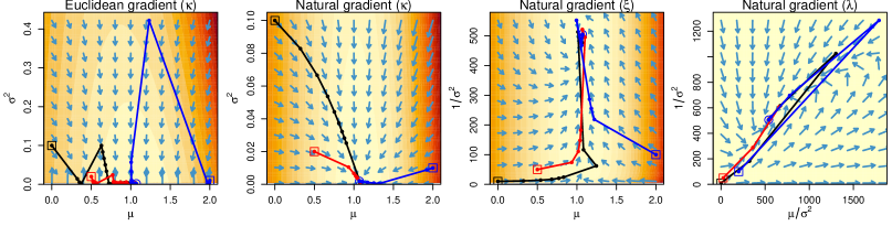
Figure 1: Gradient vector field and trajectories for gradient ascent from three starting points.

Table 2: Number of iterations in gradient ascent and smallest $\rho_{t}$ used.

Starting point Euclidean ($\kappa$) Natural ($\kappa$) Natural ($\xi$) Natural ($\lambda$) (0, 0.1) 141 (1e-05) 15 (0.01) 11 (0.01) 6 (1) (0.5, 0.02) 107 (1e-06) 12 (0.1) 8 (0.1) 5 (1) (2, 0.01) 115 (1e-06) 9 (0.01) 8 (0.1) 5 (1)

The first two plots show the contrast between Euclidean and natural gradient vector fields for the $(\mu,\sigma^{2})$ parametrization, particularly when $\sigma^{2}$ is close to zero. While natural gradients are collectively directed at the mode, Euclidean gradients have much stronger vertical components, causing zigzag trajectories that result in longer routes. The number of iterations required for Euclidean gradient ascent is an order of magnitude larger than natural gradient ascent, and a much smaller stepsize has to be used (at some point) to avoid a negative $\sigma^{2}$ update or ${\mathcal{L}}$ decreasing. Natural gradient ascent for $\lambda$ is most efficient, where a stepsize as large as 1 can be used from all starting points, indicating that reversing the order of $\mu$ and $\sigma^{2}$ updates leads to significant improvement.

6 Natural gradient updates for mean and Cholesky factor

In many applications, the lower bound cannot be computed analytically and stochastic gradient ascent based on updating the mean and Cholesky factor of the covariance/precision matrix is performed, as this allows optimization without positive definite constraints, more flexibility in choice of stepsize and reduction in computation/storage costs. However, existing updates for Cholesky factors are based on Euclidean gradients (Titsias and Lázaro-Gredilla, 2014; Tan and Nott, 2018), and we seek to derive the natural gradient counterparts. We consider two parametrizations based on Cholesky decomposition of the covariance or precision matrix. The first is $\lambda=(\mu^{T},\text{vech}(C)^{T})^{T}$ where $\Sigma=CC^{T}$ and the second is $\lambda=(\mu^{T},\text{vech}(T)^{T})^{T}$ where $\Sigma^{-1}=TT^{T}$, and $C$ and $T$ are lower triangular matrices. In these cases, $\lambda$ is not the natural parameter and we need to find the inverse Fisher information explicitly to get the natural gradient. The Fisher information for both parametrizations are block diagonal matrices with the same form. Hence the inverse can be found using a common result in (ii) of Lemma 1, while (iii) is useful in simplifying the natural gradient $F_{\lambda}^{-1}\nabla_{\lambda}{\mathcal{L}}$. The inverse Fisher information and natural gradient for these two parametrizations are presented in Theorem 1.

Lemma 1

Let $\Lambda$ be a $d\times d$ lower triangular matrix and

$$\mathfrak{I}(\Lambda)=L\{(\Lambda^{-1}\otimes\Lambda^{-T})K+I_{d}\otimes\Lambda^{-T}\Lambda^{-1}\}L^{T}.$$

If $N=(K+I_{d^{2}})/2$, then

1. $\mathfrak{I}(\Lambda)=2L(I_{d}\otimes\Lambda^{-T})N(I_{d}\otimes\Lambda^{-1})L^{T}$,

2. $\mathfrak{I}(\Lambda)^{-1}=\tfrac{1}{2}L(I_{d}\otimes\Lambda)L^{T}(LNL^{T})^{-1}L(I_{d}\otimes\Lambda^{T})L^{T}$ and

3. $\mathfrak{I}(\Lambda)^{-1}\text{vech}(G)=\text{vech}(\Lambda\bar{\bar{H}})$ for any $d\times d$ matrix $G$, where $H=\Lambda^{T}\bar{G}$.

Theorem 1

Let $\nabla_{\text{vech}(\Lambda)}{\mathcal{L}}=\text{vech}(G)$ and $H=\Lambda^{T}\bar{G}$, where $\Lambda=C$ for $\lambda=(\mu^{T},\text{vech}(C)^{T})^{T}$ and $\Lambda=T$ for $\lambda=(\mu^{T},\text{vech}(T)^{T})^{T}$. Then

$$F_{\lambda}=\begin{bmatrix}\Sigma^{-1}&0\\ 0&\mathfrak{I}(\Lambda)\end{bmatrix},\quad F_{\lambda}^{-1}=\begin{bmatrix}\Sigma&0\\ 0&\mathfrak{I}(\Lambda)^{-1}\end{bmatrix}\quad\text{and}\quad\widetilde{\nabla}_{\lambda}{\mathcal{L}}=\begin{bmatrix}\Sigma\nabla_{\mu}{\mathcal{L}}\\ \text{vech}(\Lambda\bar{\bar{H}})\end{bmatrix}.$$

Hence, the natural gradient update at iteration $t$ is

$$\Lambda^{(t+1)}=\Lambda^{(t)}+\rho_{t}\Lambda^{(t)}\bar{\bar{H}}^{(t)},\quad\mu^{(t+1)}=\mu^{(t)}+\rho_{t}\Sigma^{(t)}\nabla_{\mu}{\mathcal{L}}^{(t)}.$$

Inspired by the superior performance the natural parameter has compared to other orthogonal parametrizations in Section 5.1, we consider a one-one transformation of $\lambda=(\mu^{T},\text{vech}(T)^{T})^{T}$ in Corollary 1 akin to the natural parameter. It reveals that instead of updating $\mu$ and $T$ independently as in Theorem 1, the updated $T$ can be used to update $\mu$. Unfortunately, it is not possible to obtain similar improved updates for $C$. Proofs of Lemma 1, Theorem 1 and Corollary 1 are given in the supplement S3.

Corollary 1

Let $\xi=((T^{T}\mu)^{T},\text{vech}(T)^{T})^{T}$, $\nabla_{\text{vech}(T)}{\mathcal{L}}=\text{vech}(G)$ and $H=T^{T}\bar{G}$. Then $\widetilde{\nabla}_{\xi}{\mathcal{L}}=((T^{-1}\nabla_{\mu}{\mathcal{L}}+\bar{\bar{H}}^{T}T^{T}\mu)^{T},\text{vech}(T\bar{\bar{H}})^{T})^{T}$ and the natural gradient update at iteration $t$ is

$$T^{(t+1)}=T^{(t)}+\rho_{t}T^{(t)}\bar{\bar{H}}^{(t)},\quad\mu^{(t+1)}=\mu^{(t)}+\rho_{t}{T^{(t+1)}}^{-T}{T^{(t)}}^{-1}\nabla_{\mu}{\mathcal{L}}^{(t)}.$$

To investigate the difference between updates of $\mu$ and $T$ in Theorem 1 and Corollary 1, we consider the Poisson loglinear model in Section 5.1 again, this time fitting model 1: Sa $\sim$ Width, and model 2: Sa $\sim$ Color + Width. The largest stepsize $\rho_{t}\in\{1,0.1,0.01,...\}$ is used provided ${\mathcal{L}}$ is increasing. Figure 2 shows that updates in Corollary 1 are superior as they converge faster and are more resilient to larger stepsize.

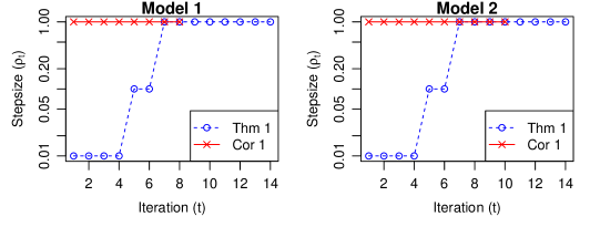
Figure 2: Stepsize $\rho_{t}$ used at each iteration of natural gradient update of $\mu$ and $T$ based on Theorem 1 and Corollary 1.

6.1 Stochastic natural gradient updates

In applications where $\nabla_{\lambda}{\mathcal{L}}$ is not analytic, we can perform stochastic natural gradient ascent using an unbiased estimate. For updates of $\mu$ and $\Sigma$, Khan et al. (2018) invoke the Theorems of Bonnet (1964) and Price (1958) to obtain unbiased estimates of $\nabla_{\mu}{\mathcal{L}}$ and $\nabla_{\Sigma}{\mathcal{L}}$. The theorems below and their proofs are given in Lin et al. (2019), and ACL is an abbreviation for absolute continuity on almost every straight line (Leoni, 2017). The second equality in Bonnet’s Theorem is also known as Stein’s Lemma (Stein, 1981). As ${\mathcal{L}}={\text{E}}_{q}[h(\theta)]$, if $\theta$ is a sample generated from $q_{\lambda}(\theta)$ at iteration $t$, then the stochastic natural gradient update of the natural parameter $\lambda$ is

$$\Sigma^{-1}\leftarrow\Sigma^{-1}-\rho_{t}\nabla^{2}_{\theta}h(\theta),\quad\mu\leftarrow\mu+\rho_{t}\Sigma\nabla_{\theta}h(\theta).$$

Bonnet’s Theorem (Stein’s Lemma)

If $\theta\sim N(\mu,\Sigma)$ and $h:\mathbbm{R}^{d}\rightarrow\mathbbm{R}$ is locally ACL and continuous, then $\nabla_{\mu}{\text{E}}_{q}[h(\theta)]={\text{E}}_{q}\left[\Sigma^{-1}(\theta-\mu)h(\theta)\right]={\text{E}}_{q}[\nabla_{\theta}h(\theta)]$.

Price’s Theorem

If $\theta\sim N(\mu,\Sigma)$, $h:\mathbbm{R}^{d}\rightarrow\mathbbm{R}$ is continuously differentiable, $\nabla_{\theta}h(\theta)$ is locally ACL and $E_{q}[h(\theta)]$ is well-defined, then

$$\nabla_{\Sigma}{\text{E}}_{q}[h(\theta)]=\tfrac{1}{2}{\text{E}}_{q}\left[\Sigma^{-1}(\theta-\mu)\nabla_{\theta}h(\theta)^{T}\right]=\tfrac{1}{2}{\text{E}}_{q}\left[\nabla_{\theta}^{2}h(\theta)\right].$$

For updates of Cholesky factors, we cannot apply Price’s Theorem directly but there are several alternatives. The score function method uses $\nabla_{\lambda}q_{\lambda}(\theta)=q_{\lambda}(\theta)\nabla_{\lambda}\log q_{\lambda}(\theta)$ to write $\nabla_{\lambda}{\mathcal{L}}={\text{E}}_{q}[\nabla_{\lambda}\log q_{\lambda}(\theta)h(\theta)]$. While widely applicable, such estimates tend to have high variance leading to slow convergence, and further variance reduction techniques are required (Paisley et al., 2012; Ranganath et al., 2014; Ruiz et al., 2016). The reparametrization trick (Kingma and Welling, 2014) introduces a differentiable transformation $\theta=\mathcal{T}_{\lambda}(z)$ so that the density $\phi(z)$ of $z$ is independent of $\lambda$. Making a variable substitution and applying chain rule, $\nabla_{\lambda}{\mathcal{L}}={\text{E}}_{\phi}[\nabla_{\lambda}\theta\,\nabla_{\theta}h(\theta)]$. Gradients estimated using the reparametrization trick typically have lower variance than the score function method (Xu et al., 2019), but yields unbiased estimates of $\nabla_{\text{vech}(C)}{\mathcal{L}}$ and $\nabla_{\text{vech}(C)}{\mathcal{L}}$ that only make use of the first derivative of $h(\theta)$ unlike Price’s Theorem.

We propose alternative unbiased estimates in terms of the second derivative of $h(\theta)$ in Theorem 2. Our results extend Bonnet’s and Price’s Theorems to gradients with respect to the Cholesky factor of the covariance/precision matrix. Lemma 2 is instrumental in proving Theorem 2 and all proofs are given in the supplement S3.

Lemma 2

If $\theta\sim N(\mu,\Sigma)$ and $h:\mathbbm{R}^{d}\rightarrow\mathbbm{R}$ is locally ACL and continuous, then ${\text{E}}_{q}\left[\{\Sigma^{-1}(\theta-\mu)(\theta-\mu)^{T}-I_{d}\}h(\theta)\right]={\text{E}}_{q}\left[\nabla_{\theta}h(\theta)(\theta-\mu)^{T}\right]$.

Theorem 2

Suppose $\theta\sim N(\mu,\Sigma)$, and $CC^{T}$ and $TT^{T}$ are Cholesky decompositions of $\Sigma$ and $\Sigma^{-1}$ respectively, where $C$ and $T$ are lower triangular matrices. Let $h:\mathbbm{R}^{d}\rightarrow\mathbbm{R}$ be continuously differentiable, and $h$ and $\nabla_{\theta}h(\theta)$ be locally ACL. Then

1. $\nabla_{\text{vech}(C)}{\mathcal{L}}={\text{E}}_{q}\text{vech}({\mathcal{G}}_{1})={\text{E}}_{q}\text{vech}({\mathcal{F}}_{1})$, where ${\mathcal{G}}_{1}=\nabla_{\theta}h(\theta)(\theta-\mu)^{T}C^{-T}$ and ${\mathcal{F}}_{1}=\nabla_{\theta}^{2}h(\theta)C$.

2. $\nabla_{\text{vech}(T)}{\mathcal{L}}={\text{E}}_{q}\text{vech}({\mathcal{G}}_{2})={\text{E}}_{q}\text{vech}({\mathcal{F}}_{2})$, where ${\mathcal{G}}_{2}=-(\theta-\mu)v^{T}$, $v=T^{-1}\nabla_{\theta}h(\theta)$ and ${\mathcal{F}}_{2}=-\Sigma\nabla_{\theta}^{2}h(\theta)T^{-T}$.

Results in Theorem 2 are obtained by first finding $\nabla_{\text{vech}(C)}{\mathcal{L}}$ and $\nabla_{\text{vech}(C)}{\mathcal{L}}$ using the score function method, which yields unbiased estimates in terms of $h(\theta)$. Applying Bonnet’s Theorem (Stein’s Lemma), we get estimates in terms of $\nabla_{\theta}h(\theta)$, which are identical to those obtained from the reparametrization trick. Finally, estimates in terms of $\nabla_{\theta}^{2}h(\theta)$ are obtained using Price’s Theorem. The reparametrization trick is thus connected to the score function method via Stein’s Lemma. Since Price’s Theorem can be derived from Bonnet’s Theorem by applying Stein’s Lemma, we are applying Stein’s Lemma repeatedly to obtain unbiased estimates in terms of even higher derivatives of $h(\theta)$. Second order estimates are undoubtedly more expensive computationally, but they can be advantageous in some situations where $\nabla^{2}_{\theta}h(\theta)$ is not excessively complex, as they are more stable when close to the optimum. Suppose $\ell(\theta)=\log p(y,\theta)$ is well approximated by a second order Taylor expansion about its mode $\hat{\theta}$. Then

$$\begin{gathered}h(\theta)\approx\ell(\hat{\theta})+\tfrac{1}{2}(\theta-\hat{\theta})^{T}\nabla_{\theta}^{2}\ell(\hat{\theta})(\theta-\hat{\theta})+\tfrac{d}{2}\log(2\pi)+\tfrac{1}{2}\log|\Sigma|+\tfrac{1}{2}(\theta-\mu)\Sigma^{-1}(\theta-\mu),\\ \nabla_{\theta}h(\theta)\approx\nabla_{\theta}^{2}\ell(\hat{\theta})(\theta-\hat{\theta})+\Sigma^{-1}(\theta-\mu),\qquad\nabla_{\theta}^{2}h(\theta)\approx\nabla_{\theta}^{2}\ell(\hat{\theta})+\Sigma^{-1},\end{gathered}$$

which leads to the estimators,

$$\begin{gathered}{\mathcal{G}}_{1}\approx\{\nabla_{\theta}^{2}\ell(\hat{\theta})(\theta-\hat{\theta})+\Sigma^{-1}(\theta-\mu)\}(\theta-\mu)^{T}C^{-T},\quad{\mathcal{F}}_{1}\approx\nabla_{\theta}^{2}\ell(\hat{\theta})C+C^{-T},\\ {\mathcal{G}}_{2}\approx-(\theta-\mu)\{(\theta-\hat{\theta})^{T}\nabla_{\theta}^{2}\ell(\hat{\theta})T^{-T}+(\theta-\mu)^{T}T\},\quad{\mathcal{F}}_{2}\approx-\Sigma\nabla_{\theta}^{2}\ell(\hat{\theta})T^{-T}-T^{-T}.\end{gathered}$$

While ${\mathcal{F}}_{1}$ and ${\mathcal{F}}_{2}$ are independent of $\theta$ and hence have (close to) zero variances, ${\mathcal{G}}_{1}$ and ${\mathcal{G}}_{2}$ are subjected to variation arising from simulation of $\theta$ from $q_{\lambda}(\theta)$. Hence ${\mathcal{F}}_{1}$ and ${\mathcal{F}}_{2}$ are more stable close to the optimum where ${\mathcal{L}}$ will be approximately quadratic.

Stochastic variational algorithms obtained using Theorem 2 are outlined in Tables 3 and 4, and we have applied Corollary 1 in the update of $\mu$ in Algorithm 2N. Algorithms based on Euclidean and natural gradients are placed side-by-side for ease of comparison. Those based on natural gradients have an additional step for computing $\bar{\bar{H}}$ and the updates involve some form of scaling, which can help to improve convergence.

Table 3: Stochastic variational algorithms for updating $\mu$ and $C$.

Algorithm 1E (Euclidean gradient) Algorithm 1N (Natural gradient) Initialize $\mu$ and $C$. For $t=1,2,\dots$, 1. Generate $z\sim{\text{N}}(0,I_{d})$ and compute $\theta=Cz+\mu$. 2. Find $\bar{G}$ where $G=\nabla_{\theta}h(\theta)z^{T}$ or $G=\nabla_{\theta}^{2}h(\theta)C$. 3. Update $\mu\leftarrow\mu+\rho_{t}\nabla_{\theta}h(\theta)$. 4. Update $C\leftarrow C+\rho_{t}\bar{G}$. 3. Update $\mu\leftarrow\mu+\rho_{t}CC^{T}\nabla_{\theta}h(\theta)$. 4. Find $\bar{\bar{H}}$ where $H=C^{T}\bar{G}$. 5. Update $C\leftarrow C+\rho_{t}C\bar{\bar{H}}$.

Table 4: Stochastic variational algorithms for updating $\mu$ and $T$.

Algorithm 2E (Euclidean gradient) Algorithm 2N (Natural gradient) Initialize $\mu$ and $T$. For $t=1,2,\dots$, 1. Generate $z\sim{\text{N}}(0,I_{d})$ and compute $\theta=T^{-T}z+\mu$. 2. Find $\bar{G}$ where $G=-T^{-T}zv^{T}$, $v=T^{-1}\nabla_{\theta}h(\theta)$ or $G=-T^{-T}T^{-1}\nabla_{\theta}^{2}h(\theta)T^{-T}$. 3. Update $\mu\leftarrow\mu+\rho_{t}\nabla_{\theta}h(\theta)$. 4. Update $T\leftarrow T+\rho_{t}\bar{G}$. 3. Find $\bar{\bar{H}}$ where $H=T^{T}\bar{G}$. 4. Update $T\leftarrow T+\rho_{t}T\bar{\bar{H}}$. 5. Update $\mu\leftarrow\mu+\rho_{t}T^{-T}v$.

7 Imposing sparsity

For high-dimensional models, it may be useful to impose sparsity on the covariance or precision matrix, and hence on their Cholesky factors to increase efficiency. For Algorithms 1E and 2E, updates of sparse Cholesky factors can be obtained simply by extracting entries in the Euclidean gradients that correspond to nonzero entries in the Cholesky factor, but the same may not apply to natural gradients due to premultiplication by the Fisher information. As illustration, suppose $\lambda=(\lambda_{1}^{T},\lambda_{2}^{T})^{T}$ and the Fisher information, Euclidean gradient and natural gradient for this partitioning are respectively

$$F_{\lambda}=\begin{bmatrix}F_{11}&F_{12}\\ F_{21}&F_{22}\end{bmatrix},\quad g_{\lambda}=\begin{bmatrix}g_{1}\\ g_{2}\end{bmatrix},\quad\widetilde{g}_{\lambda}=F_{\lambda}^{-1}g_{\lambda}=\begin{bmatrix}\widetilde{g}_{1}\\ \widetilde{g}_{2}\end{bmatrix}.$$

By block matrix inversion, $\widetilde{g}_{1}=F_{11}^{-1}g_{1}-F_{11}^{-1}F_{12}\widetilde{g}_{2}$. If we fix $\lambda_{2}=0$ ($\lambda_{2}$ is no longer an unknown parameter), then the natural gradient for updating $\lambda_{1}$ is just $F_{11}^{-1}g_{1}$, which is equal to $\widetilde{g}_{1}+F_{11}^{-1}F_{12}\widetilde{g}_{2}$, not $\widetilde{g}_{1}$. Thus, we cannot update $\lambda_{1}$ simply by extracting $\widetilde{g}_{1}$.

In this section, we derive efficient natural gradient updates of the Cholesky factors in two cases, (i) the covariance matrix has a block diagonal structure corresponding to the product density assumption in variational Bayes and (ii) the precision matrix reflects the posterior conditional independence structure in a hierarchical model where local variables are independent conditional on the global variables.

7.1 Block diagonal covariance structure

Let $q_{\lambda}(\theta)=\prod_{i=1}^{N}q_{\lambda_{i}}(\theta_{i})$ for some partitioning $\theta=(\theta_{1}^{T},\dots,\theta_{N}^{T})^{T}$, where $\theta_{i}\sim{\text{N}}(\mu_{i},\Sigma_{i})$. Then $\Sigma={\text{blockdiag}}(\Sigma_{1},\dots,\Sigma_{N})$ and $\mu=(\mu_{1}^{T},\dots,\mu_{N}^{T})^{T}$. Let $C_{i}C_{i}^{T}$ be the Cholesky decomposition of $\Sigma_{i}$, where $C_{i}$ is a lower triangular matrix for $i=1,\dots,N$, and $C={\text{blockdiag}}(C_{1},\dots,C_{N})$. For the parametrization $\lambda=(\mu^{T},\text{vech}(C_{1})^{T},\dots,\text{vech}(C_{N})^{T})^{T}$, the Fisher information, $F_{\lambda}={\text{blockdiag}}(\Sigma^{-1},\mathfrak{I}(C_{1}),\dots,\mathfrak{I}(C_{N}))$, where $\mathfrak{I}(\cdot)$ is defined in Lemma 1. Let $\nabla_{\text{vech}(C_{i})}{\mathcal{L}}=\text{vech}(G_{i})$ and $H_{i}=C_{i}^{T}\bar{G}_{i}$ for $i=1,\dots,N$. Then it follows from Lemma 1 that the natural gradient,

$$\widetilde{\nabla}_{\lambda}{\mathcal{L}}=F_{\lambda}^{-1}\nabla_{\lambda}{\mathcal{L}}=\begin{bmatrix}\Sigma&0&\dots&0\\ 0&\mathfrak{I}(C_{1})^{-1}&\dots&0\\ \vdots&\vdots&\ddots&\vdots\\ 0&0&\dots&\mathfrak{I}(C_{N})^{-1}\\ \end{bmatrix}\begin{bmatrix}\nabla_{\mu}{\mathcal{L}}\\ \text{vech}(\bar{G}_{1})\\ \vdots\\ \text{vech}(\bar{G}_{N})\end{bmatrix}=\begin{bmatrix}\Sigma\nabla_{\mu}{\mathcal{L}}\\ \text{vech}(C_{1}\bar{\bar{H}}_{1})\\ \vdots\\ \text{vech}(C_{N}\bar{\bar{H}}_{N})\end{bmatrix}.$$

This explicit expression of the natural gradient reveals the sparse structures of matrices that underlie its computation. Let $\bar{G}={\text{blockdiag}}(\bar{G}_{1},\dots,\bar{G}_{N})$, $H={\text{blockdiag}}(H_{1},\dots,H_{N})$ and $\bar{\bar{H}}={\text{blockdiag}}(\bar{\bar{H}}_{1},\dots,\bar{\bar{H}}_{N})$. Then $H=C^{T}\bar{G}$ and $C\bar{\bar{H}}={\text{blockdiag}}(C_{1}\bar{\bar{H}}_{1},\dots,C_{N}\bar{\bar{H}}_{N})$. Thus $C$, $\bar{G}$, $\bar{\bar{H}}$ and $C\bar{\bar{H}}$ have the same sparse block lower triangular structure (see Figure 3), which is useful in improving storage and computational efficiency.

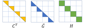
Figure 3: Shaded regions represent nonzero entries in $C^{T}$, $\bar{G}$ and $H=C^{T}\bar{G}$ ($N=4$).

If the Euclidean gradient $\nabla_{\lambda}{\mathcal{L}}$ is intractable, then unbiased estimates of $\nabla_{\text{vech}(C_{i})}{\mathcal{L}}$ can be obtained using Theorem 2 (i). As $C={\text{blockdiag}}(C_{1},\dots,C_{N})$, we only have to extract the entries in ${\mathcal{G}}_{1}$ and ${\mathcal{F}}_{1}$ that correspond to $C_{1},\dots,C_{N}$ on the block diagonal. For $i=1,\dots,N$,

$$\nabla_{\text{vech}(C_{i})}{\mathcal{L}}={\text{E}}_{q}\text{vech}\{\nabla_{\theta_{i}}h(\theta)(\theta_{i}-\mu_{i})^{T}C_{i}^{-T}\}={\text{E}}_{q}\text{vech}(\nabla_{\theta_{i}}^{2}h(\theta)C_{i}).$$

The resulting stochastic variational algorithm 1S is outlined in Table 5.

Table 5: Stochastic natural gradient algorithms incorporating sparsity.

Algorithm 1S (Update $\mu$ and $C$) Algorithm 2S (Update $\mu$ and $T$) Initialize $\mu$ and $C={\text{blockdiag}}(C_{1},\dots,C_{N})$. For $t=1,2,\dots$, 1. Generate $z\sim{\text{N}}(0,I_{d})$ and
compute $\theta=Cz+\mu$. 2. Find $\bar{G}={\text{blockdiag}}(\bar{G}_{1},\dots,\bar{G}_{N})$ where $G_{i}=\nabla_{\theta_{i}}h(\theta)(\theta_{i}-\mu_{i})^{T}C_{i}^{-T}$ or $\nabla_{\theta_{i}}^{2}h(\theta)C_{i}$. 3. Compute $\bar{\bar{H}}$ where $H=C^{T}\bar{G}$. 4. Update $\mu\leftarrow\mu+\rho_{t}CC^{T}\nabla_{\theta}h(\theta)$. 5. Update $C\leftarrow C+\rho_{t}C\bar{\bar{H}}$. Initialize $\mu$ and $T$ in (3). For $t=1,2,\dots$, 1. Generate $z\sim{\text{N}}(0,I_{d})$ and
compute $\theta=T^{-T}z+\mu$. 2. Find $\bar{G}$ where $G$ comprises blocks in $uv^{T}$ or $T_{d}^{-T}T^{-1}\nabla_{\theta}^{2}h(\theta)T^{-T}$ that correspond to nonzero blocks in $T$. 3. Compute $\bar{\bar{H}}$ where $H=T_{d}^{T}\bar{G}$. 4. Update $T\leftarrow T+\rho_{t}T\bar{\bar{H}}$. 5. Update $\mu\leftarrow\mu+\rho_{t}T^{-T}v$.

7.2 Sparse precision matrix

Consider a hierarchical model where the local variables specific to individual observations, $\theta_{1},\dots,\theta_{n}$, are independent of each other conditional on the global variables shared across all observations, $\theta_{g}$. Then the joint density is of the form,

$$p(y,\theta)=p(\theta_{g})\prod_{i=1}^{n}p(y_{i}|\theta_{i},\theta_{g})p(\theta_{i}|\theta_{g}),$$

where $y=(y_{1},\dots,y_{n})^{T}$, $\theta=(\theta_{1}^{T},\dots,\theta_{n}^{T},\theta_{g}^{T})^{T}$ and $p(\theta_{g})$ is a prior density for the global variables. For this model, $\theta_{1},\dots,\theta_{n}$ are conditionally independent given $\theta_{g}$ a posteriori. To mirror this conditional independence structure in the posterior distribution, let the the Cholesky factor of precision matrix $\Sigma^{-1}$ be of the form

$$T=\begin{bmatrix}T_{1}&\dots&0&0\\ \vdots&\ddots&\vdots&\vdots\\ 0&\dots&T_{n}&0\\ T_{g1}&\dots&T_{gn}&T_{g}\end{bmatrix},$$ (3)

where $T_{1},\dots,T_{n},T_{g}$ are lower triangular matrices. Let $\mu=(\mu_{1}^{T},\dots,\mu_{n}^{T},\mu_{g}^{T})^{T}$ be the corresponding partitioning, $\Sigma_{g}^{-1}=T_{g}T_{g}^{T}$ and $\Sigma_{i}^{-1}=T_{i}T_{i}^{T}$ for $i=1,\dots,n$. Then $q_{\lambda}(\theta)=q(\theta_{g})\prod_{i=1}^{n}q(\theta_{i}|\theta_{g})$, where $q(\theta_{g})$ is ${\text{N}}(\mu_{g},\Sigma_{g})$ and $q(\theta_{i}|\theta_{g})$ is ${\text{N}}(\mu_{i}-T_{i}^{-T}T_{gi}^{T}(\theta_{g}-\mu_{g}),\Sigma_{i})$ for $i=1,\dots,n$.

Consider

$$\lambda=(\mu^{T},\text{vech}(T_{1})^{T},\text{vec}(T_{g1})^{T},\dots,\text{vech}(T_{n})^{T},\text{vec}(T_{gn})^{T},\text{vech}(T_{g})^{T})^{T}.$$

For this ordering, the Fisher information has a block diagonal structure and can be inverted easily. By using Lemma 1 and block matrix inversion, we show in the supplement S4 that $F_{\lambda}^{-1}={\text{blockdiag}}(\Sigma,F_{1}^{-1},\dots,F_{n}^{-1},\mathfrak{I}(T_{g})^{-1})$, where

$$F_{i}^{-1}=\begin{bmatrix}\mathfrak{I}(T_{i})^{-1}&\mathfrak{I}(T_{i})^{-1}L(I\otimes T_{i}^{-T}T_{gi}^{T})\\ \cdot&(I\otimes\Sigma_{g}^{-1})+(I\otimes T_{gi}T_{i}^{-1})L^{T}\mathfrak{I}(T_{i})^{-1}L(I\otimes T_{i}^{-T}T_{gi}^{T})\end{bmatrix}.$$

Let $\nabla_{\text{vech}(T_{i})}{\mathcal{L}}=\text{vech}(A_{i})$, $\nabla_{\text{vec}(T_{gi})}{\mathcal{L}}=\text{vec}(G_{gi})$ for $i=1,\dots,n$ and $\nabla_{\text{vech}(T_{g})}{\mathcal{L}}=\text{vech}(G_{g})$. Applying Lemma 1, the natural gradient is

$$\widetilde{\nabla}_{\lambda}{\mathcal{L}}=F_{\lambda}^{-1}\begin{bmatrix}\nabla_{\mu}{\mathcal{L}}\\ \begin{bmatrix}\text{vech}(A_{i})\\ \text{vec}(G_{gi})\\ \end{bmatrix}_{i=1:n}\\ \text{vech}(G_{g})\end{bmatrix}=\begin{bmatrix}\Sigma\nabla_{\mu}{\mathcal{L}}\\ \begin{bmatrix}\text{vech}(T_{i}\bar{\bar{H}}_{i})\\ \text{vec}(T_{gi}\bar{\bar{H}}_{i}+\Sigma_{g}^{-1}G_{gi})\\ \end{bmatrix}_{i=1:n}\\ \text{vech}(T_{g}\bar{\bar{H}}_{g})\end{bmatrix},$$

where $[a_{i}]_{i=1:n}=(a_{1}^{T},\dots,a_{n}^{T})^{T}$, $H_{g}=T_{g}^{T}\bar{G}_{g}$, $G_{i}=A_{i}+T_{i}^{-T}T_{gi}^{T}G_{gi}$ and $H_{i}=T_{i}^{T}\bar{G}_{i}$ for $i=1,\dots,n$. To compute the natural gradient in practice, we can define

$$G=\begin{bmatrix}G_{1}&\dots&0&0\\ \vdots&\ddots&\vdots&\vdots\\ 0&\dots&G_{n}&0\\ G_{g1}&\dots&G_{gn}&G_{g}\end{bmatrix},\quad H=T_{d}^{T}\bar{G}=\begin{bmatrix}H_{1}&\dots&0&0\\ \vdots&\ddots&\vdots&\vdots\\ 0&\dots&H_{n}&0\\ T_{g}^{T}G_{g1}&\dots&T_{g}^{T}G_{gn}&H_{g}\end{bmatrix},$$

where $T_{d}={\text{blockdiag}}(T_{1},\dots,T_{n},T_{g})$ consists only of the diagonal blocks in $T$. Then

$$T\bar{\bar{H}}=\begin{bmatrix}T_{1}\bar{\bar{H}}_{1}&\dots&0&0\\ \vdots&\ddots&\vdots&\vdots\\ 0&\dots&T_{n}\bar{\bar{H}}_{n}&0\\ T_{g1}\bar{\bar{H}}_{1}+T_{g}T_{g}^{T}G_{g1}&\dots&T_{gn}\bar{\bar{H}}_{n}+T_{g}T_{g}^{T}G_{gn}&T_{g}\bar{\bar{H}}_{g}\end{bmatrix},$$

yields all the necessary components in the natural gradient. In addition, $\bar{G}$, $\bar{\bar{H}}$ and $T\bar{\bar{H}}$ all have the same sparse structure as $T$.

7.3 Stochastic natural gradient for sparse precision matrix

If $\nabla_{\lambda}{\mathcal{L}}$ is not analytic, unbiased estimates of $\nabla_{\lambda}{\mathcal{L}}$ can be obtained from Theorem 2 (ii) by extracting entries in ${\mathcal{G}}_{2}$ and ${\mathcal{F}}_{2}$ that correspond to nonzero entries in $T$. As the $\theta_{i}$s are conditionally independent in both $p(y,\theta)$ and $q_{\lambda}(\theta)$, $\nabla_{\theta_{i},\theta_{j}}^{2}h(\theta)=0$ if $i\neq j$ and $\nabla_{\theta}^{2}h(\theta)$ is also sparse. Let $u=(u_{1}^{T},\dots,u_{n}^{T},u_{g}^{T})^{T}=T_{d}^{-T}z$ where $z=T^{T}(\theta-\mu)$, $v=(v_{1}^{T},\dots,v_{n}^{T},v_{g}^{T})^{T}=T^{-1}\nabla_{\theta}h(\theta)$ and

$$U_{gg} =\Sigma_{g}\bigg{(}\nabla_{\theta_{g}}^{2}h(\theta)-\sum_{i=1}^{n}T_{gi}T_{i}^{-1}\nabla_{\theta_{i},\theta_{g}}^{2}h(\theta)\bigg{)}T_{g}^{-T},$$

$$U_{gi} =\Sigma_{g}\{\nabla_{\theta_{g},\theta_{i}}^{2}h(\theta)-T_{gi}T_{i}^{-1}\nabla_{\theta_{i}}^{2}h(\theta)\}T_{i}^{-T}\quad(i=1,\dots,n).$$

In the supplement S4, we show that for $i=1,\dots,n$,

$$\nabla_{\text{vech}(T_{i})}{\mathcal{L}} ={\text{E}}_{q}\text{vech}\{(T_{i}^{-T}T_{gi}u_{g}-u_{i})v_{i}^{T}\}={\text{E}}_{q}\text{vech}(T_{i}^{-T}T_{gi}^{T}U_{gi}-\Sigma_{i}\nabla_{\theta_{i}}^{2}h(\theta)T_{i}^{-T}),$$

$$\nabla_{\text{vec}(T_{gi})}{\mathcal{L}} =-{\text{E}}_{q}\text{vec}(u_{g}v_{i}^{T})=-{\text{E}}_{q}\text{vec}(U_{gi}),$$

$$\nabla_{\text{vech}(T_{g})}{\mathcal{L}} =-{\text{E}}_{q}\text{vech}(u_{g}v_{g}^{T})={\text{E}}_{q}\text{vech}\bigg{(}\sum_{i=1}^{n}U_{gi}T_{gi}^{T}T_{g}^{-T}-U_{gg}\bigg{)}.$$

Using the above results, we can obtain unbiased estimates of the natural gradient in terms of $\nabla_{\theta}h(\theta)$ by setting

$$G_{g}=-u_{g}v_{g}^{T},\;\;G_{gi}=-u_{g}v_{i}^{T},\;\;G_{i}=-u_{i}v_{i}^{T}\quad(i=1,\dots,n).$$

On the other hand, unbiased estimates in terms of $\nabla_{\theta}^{2}h(\theta)$ can be obtained by setting

$$G_{g}=\sum_{i=1}^{n}U_{gi}T_{gi}^{T}T_{g}^{-T}-U_{gg},\;\;G_{gi}=-U_{gi}\;\;G_{i}=-\Sigma_{i}\nabla_{\theta_{i}}^{2}h(\theta)T_{i}^{-T}\quad(i=1,\dots,n).$$

In practice, we can compute $G$ by finding the blocks in $uv^{T}$ or $T_{d}^{-T}T^{-1}\nabla_{\theta}^{2}h(\theta)T^{-T}$ that correspond to nonzero blocks in $T$. The overall procedure is outlined in Algorithm 2S (Table 5). Compared with 2N, the computation of $\bar{G}$ and $\bar{\bar{H}}$ differ in sparsity and some usage of $T_{d}$ instead of $T$. Further derivation details are given in the supplement S4.

8 Stochastic normalized natural gradient ascent with momentum

Next, we discuss the choice of stepsize $\rho_{t}$ in stochastic natural gradient ascent. For high-dimensional models, it is particularly important to use an adaptive stepsize that is robust to noisy gradient information. Some popular approaches include Adagrad (Duchi et al., 2011), Adadelta (Zeiler, 2012) and Adam (Kingma and Ba, 2015), which compute elementwise adaptive learning rates using past gradients. Notably, Adam introduces momentum by computing the exponential moving average of the gradient ($m_{t}$) and elementwise squared gradient ($v_{t}$), and corrects for the bias due to initializing $m_{t}$ and $v_{t}$ at 0 using $\widehat{m}_{t}$ and $\widehat{v}_{t}$ (Table 6). The effective step is $\alpha\widehat{m}_{t}/(\sqrt{\widehat{v}_{t}}+\epsilon)$, where $\epsilon$ is a small constant that is added to avoid division by zero.

Table 6: Adam and Snngm (scalar functions are performed elementwise on vectors).

Adam (Kingma and Ba, 2015) Snngm Default: $\alpha=0.001$, $\beta_{1}=0.9$, $\beta_{2}=0.999$, $\epsilon=10^{-8}$. Initialize $m_{0}=0$, $v_{0}=0$ and $\lambda^{(1)}$. For $t=1,2,\dots$, 1. Compute gradient estimate $\widehat{g}_{t}$. 2. $m_{t}=\beta_{1}m_{t-1}+(1-\beta_{1})g_{t}$. 3. $v_{t}=\beta_{2}v_{t-1}+(1-\beta_{2})g_{t}^{2}$. 4. $\widehat{m}_{t}=m_{t}/(1-\beta_{1}^{t})$ and $\widehat{v}_{t}=v_{t}/(1-\beta_{2}^{t})$. 5. $\lambda^{(t+1)}=\lambda^{(t)}+\alpha\widehat{m}_{t}/(\sqrt{\widehat{v}_{t}}+\epsilon)$. Default: $\alpha=0.001\sqrt{\ell_{\lambda}}$ where $\ell_{\lambda}$ is length of $\lambda$, $\beta=0.9$. Initialize $m_{0}=0$ and $\lambda^{(1)}$. For $t=1,2,\dots$, 1. Compute natural gradient estimate $\widetilde{g}_{t}$. 2. $m_{t}=\beta m_{t-1}+(1-\beta)\widetilde{g}_{t}/\|\widetilde{g}_{t}\|$. 3. $\widehat{m}_{t}=m_{t}/(1-\beta^{t})$. 4. $\lambda^{(t+1)}=\lambda^{(t)}+\alpha\widehat{m}_{t}$.

8.1 Motivation of Snngm and its difference from Adam

Despite Adam’s wide applicability, we observe that use of natural gradients with Adam fails to yield significant improvement in convergence compared to Euclidean gradients. There are several factors that contribute to this phenomenon. Adam can be interpreted as a sign-based variance adapted approach (Balles and Hennig, 2018), since (ignoring $\epsilon$) the update step can be expressed as

$$\alpha\frac{\text{sign}(\widehat{m}_{t})}{\sqrt{\widehat{v}_{t}/\widehat{m}_{t}}}\approx\alpha\frac{\text{sign}(\widehat{m}_{t})}{\sqrt{{\text{E}}(g_{t}^{2})/{\text{E}}(g_{t})^{2}}}=\alpha\frac{\text{sign}(\widehat{m}_{t})}{\sqrt{1+{\text{Var}}(g_{t})/{\text{E}}(g_{t})^{2}}}.$$

The update direction is thus given by the sign of $\widehat{m}_{t}$, while the per dimension magnitude is bounded by $\alpha$ and reduced correspondingly when there is high uncertainty (measured by the relative variance ${\text{Var}}(g_{t})/{\text{E}}(g_{t})^{2}$). Moreover, experiments conducted by Balles and Hennig (2018) indicate that the sign aspect is dominant. If we replace Euclidean gradient estimate $\widehat{g}_{t}$ by natural gradient estimate $\tilde{g}_{t}$, then Adam will update by focusing on the sign information in $\tilde{g}_{t}$ while the scaling obtained via the Fisher information will be neglected to a large extent. Loss of scale information is compounded by variance adaption performed on a per dimension basis.

To overcome these issues, we propose stochastic normalized natural gradient ascent with momentum (Snngm), which is outlined in Table 6. If we exclude momentum by setting $\beta=0$, then the update step is $\alpha\widetilde{g}_{t}/\|\widetilde{g}_{t}\|$, where $\|\cdot\|$ represents the Euclidean norm. The norm of this step is fixed at $\alpha$, while the effective stepsize is $\rho_{t}=\alpha/\|\widetilde{g}_{t}\|$. The same stepsize is used for all parameters to preserve the scaling by the inverse Fisher information. In the initial stage of optimization when $\lambda$ is far from the mode, $\rho_{t}$ will be small as the gradient tends to be large in magnitude. This is important for stability especially if the initialization is far from the mode. As $\lambda$ approaches the optimum, $\rho_{t}$ increases as the gradient tends to zero. Normalized natural gradient ascent is thus able to avoid slow convergence close to the mode and is also effective at evading saddle points (Hazan et al., 2015). As the true natural gradient is unknown, we inject momentum using the exponential moving average for robustness against noisy gradients. In Table 6, we set the default $\alpha=0.001\ell_{\lambda}$ where $\ell_{\lambda}$ is the length of $\lambda$, because $\|\widetilde{g}_{t}\|$ tends to increase with $\ell_{\lambda}$ and scaling up $\alpha$ proportionally prevents the stepsize from becoming too small in high-dimensional problems. Further tuning of $\alpha$ may be desired depending on the problem but 0.001$\ell_{\lambda}$ is a good starting point.

To illustrate the difference in performance between Adam and Snngm, we consider the intercept-only loglinear model in Section 5.1 again. Figure 4 shows the gradient vector fields and trajectories of Adam or Snngm run using default settings in Table 6 from the same starting points. Use of natural gradients did not lead to any improvements in Adam. Instead, more iterations were required and the run starting from (2, 0.01) was terminated due to a negative $\sigma^{2}$ update. The second plot also indicates that Adam does not follow the flow of natural gradients closely unlike Snngm in the third plot. This is likely caused by the loss of scale information in Adam as discussed previously. On the other hand, the number of iterations was reduced by about three times using Snngm.

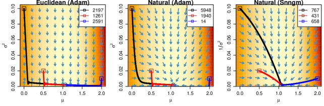
Figure 4: Gradient vector field and trajectories of Adam and Snngm from three starting points. Legend shows the total number of iterations.

8.2 Convergence of Snngm

Next, we analyze the convergence of Snngm under four assumptions, of which the first three are similar to that made by Défossez et al. (2020) in proving the convergence of Adam. Let $g_{t}=\nabla_{\lambda}{\mathcal{L}}(\lambda^{(t)})$ be the Euclidean gradient at $\lambda^{(t)}$ and $\widehat{g}_{t}=\widehat{\nabla}_{\lambda}{\mathcal{L}}(\lambda^{(t)})$ be an unbiased estimate such that ${\text{E}}_{q}(\widehat{g}_{t})=g_{t}$. In addition, let $F_{t}=F_{\lambda}(\lambda^{(t)})$ and $\widetilde{g}_{t}=F_{t}^{-1}\widehat{g}_{t}$ be an unbiased estimate of the natural gradient. The assumptions are as follows.

(A1)

${\mathcal{L}}(\lambda)\leq{\mathcal{L}}^{*}$ $\forall\lambda\in\mathbb{R}^{d}$.

(A2)

$\|\widehat{\nabla}_{\lambda}{\mathcal{L}}(\lambda)\|\leq R$ $\forall\lambda\in\mathbb{R}^{d}$.

(A3)

${\mathcal{L}}(\lambda)$ is $L$-Lipschitz smooth: $\exists$ a constant $L>0$ such that $\|\nabla_{\lambda}{\mathcal{L}}(\lambda^{\prime})-\nabla_{\lambda}{\mathcal{L}}(\lambda)\|\leq L\|\lambda^{\prime}-\lambda\|$ $\forall\;\lambda,\lambda^{\prime}\in\mathbb{R}^{d}$.

(A4)

$0<R_{1}\leq{\text{ev}}(F_{\lambda})\leq R_{2}$ $\forall\lambda\in\mathbb{R}^{d}$, where ${\text{ev}}(F_{\lambda})$ denotes the eigenvalues of $F_{\lambda}$.

Following Défossez et al. (2020), let $\tau$ be a random index such that $\text{P}(\tau=j)\propto 1-\beta^{T-j+1}$ for $j\in\{1,\dots,T\}$. The proportionality constant,

$$C=\sum_{j=1}^{T}(1-\beta^{T-j+1})=T-\frac{\beta(1-\beta^{T})}{1-\beta}\geq T-\frac{\beta}{1-\beta}=\widetilde{T}.$$

For the distribution of $\tau$, almost all values of $j$ are sampled uniformly except that the last few are sampled less often. For instance, Figure 5 shows the value of $1-\beta^{T-j+1}$ for $T=10000$ and $\beta=0.9$. All values are greater than 0.99 except for the last 43 of them.

Figure 5: Value of $1-\beta^{T-j+1}$ for $j=1,\dots,T$ where $T=10000$.

Theorem 3 provides bounds for the expected squared norm of the gradient at iteration $\tau$ in Snngm under assumptions (A1)–(A4). The proof of Theorem 3 is given in the supplement S5. If we assume $T\gg\beta/(1-\beta)$, then $\widetilde{T}\approx T$. Setting $\alpha=1/\sqrt{T}$ then yields an $O(1/\sqrt{T})$ convergence rate.

Theorem 3

In Snngm, under assumptions (A1)–(A4) and for any $T>\beta/(1-\beta)$,

$${\text{E}}\|g_{\tau}\|^{2}\leq\frac{RR_{2}}{R_{1}}\left\{\frac{{\mathcal{L}}^{*}-{\mathcal{L}}(\lambda^{(1)})}{\widetilde{T}\alpha}+\frac{TL\alpha}{\widetilde{T}}\left(\frac{\beta}{1-\beta}+\frac{1}{2}\right)\right\}.$$

9 Applications

We apply proposed methods to logistic regression and generalized linear mixed models (GLMMs). A Gaussian variational approximation with a full or diagonal covariance matrix is considered for logistic regression, while a block diagonal covariance or sparse precision matrix is used for GLMMs. The stepsize is computed using Adam or Snngm, and we compare the efficiency and accuracy of algorithms based on Euclidean versus natural gradient. Parameters for Adam and Snngm are set at default values in Table 6, except that $\alpha$ for Snngm is adjusted to $0.01\sqrt{\ell_{\lambda}}$ for algorithms 2N and 2S that update the Cholesky factor of the precision matrix. This adjustment is required likely due to the difference in scale between covariance and precision matrices. We initialize $\mu=0$ and $C=0.1I$ or equivalently $T=10I$ unless stated otherwise.

At each iteration $t$, we compute an unbiased estimate $\widehat{{\mathcal{L}}}_{t}=h(\theta^{(t)})$ of ${\mathcal{L}}$. To assess convergence, we average these estimates over every 1000 iterations and fit a least square regression line to the past three means (Tan, 2021). The algorithm is terminated once the gradient is less than 0.01. At termination (iteration $T$), we compute an estimate $\hat{{\mathcal{L}}}$ of ${\mathcal{L}}$, as the mean of $h(\theta^{(t)})$ over 1000 simulations of $\theta^{(t)}$ from $q_{\lambda^{(T)}}(\theta)$. Since our goal is to maximize ${\mathcal{L}}$, an algorithm with a higher $\hat{{\mathcal{L}}}$ is regarded as providing a better estimate of $\lambda$. The code is written in Julia (Bezanson et al., 2017) and is available as supplementary material. All experiments are run on an Intel Core i9-9900K CPU @ 3.60GHz.

9.1 Logistic regression

Given a dataset $\{(x_{i},y_{i})|i=1,\dots,n\}$ where $x_{i}\in\mathbb{R}^{d}$ and $y_{i}\in\{0,1\}$, we consider the model, $\text{logit}(p_{i})=x_{i}^{T}\theta$, where $y_{i}\sim\text{Bernoulli}(p_{i})$. It is assumed that $x_{i}$ contains an intercept. The regression coefficient $\theta$ is assigned a prior ${\text{N}}(0,\sigma_{0}^{2}I)$, where $\sigma_{0}=10$, and the posterior density of $\theta$ is approximated by ${\text{N}}(\mu,\Sigma)$. The expression of $\log p(y,\theta)$ and its first and second order derivatives are given in the supplement S6.

Table 7: Logistic regression: Number of iterations ($T$) in thousands, average lower bound $\hat{{\mathcal{L}}}$ at termination and runtime in seconds.

German Heart ICU First order $T$ $\hat{{\mathcal{L}}}$ time $T$ $\hat{{\mathcal{L}}}$ time $T$ $\hat{{\mathcal{L}}}$ time Full Cov Euclidean (Adam) 14 -627.5 6.1 13 -144.1 1.0 17 -115.3 1.4 Natural (Adam) 8 -625.9 5.7 9 -144.1 0.8 10 -115.2 1.0 Natural (Snngm) 5 -625.7 2.9 6 -144.0 0.4 7 -115.2 0.5 Diag Cov Euclidean (Adam) 16 -640.5 2.1 23 -148.6 0.3 22 -123.0 0.3 Natural (Adam) 15 -640.7 2.0 23 -148.6 0.4 22 -123.0 0.4 Natural (Snngm) 14 -639.7 1.9 13 -148.8 0.2 16 -122.9 0.2 Full Prec Euclidean (Adam) 44 -626.0 18.5 21 -144.0 1.6 24 -115.2 1.9 Natural (Adam) 27 -625.6 18.5 22 -144.0 2.2 23 -115.2 2.4 Natural (Snngm) 8 -625.7 4.8 7 -144.1 0.5 6 -115.3 0.4 Second order Full Cov Euclidean (Adam) 13 -625.6 11.5 13 -144.0 1.3 16 -115.2 1.5 Natural (Adam) 8 -625.6 9.9 10 -144.1 1.3 13 -115.2 1.7 Natural (Snngm) 4 -625.6 4.8 4 -144.0 0.4 4 -115.2 0.4 Diag Cov Euclidean (Adam) 15 -640.6 3.9 23 -148.6 0.6 22 -123.0 0.6 Natural (Adam) 15 -640.5 3.7 23 -148.6 0.7 22 -122.9 0.6 Natural (Snngm) 14 -639.9 3.5 13 -148.8 0.3 18 -122.6 0.5 Full Prec Euclidean (Adam) 17 -625.6 16.6 16 -144.0 3.0 21 -115.2 3.9 Natural (Adam) 15 -625.6 20.9 16 -144.0 4.3 16 -115.2 4.3 Natural (Snngm) 4 -625.6 4.9 4 -144.0 0.9 6 -115.3 1.4

We consider three datasets. The German credit ($n=1000$, $d=49$) and Heart ($n=270$, $d=19$) data are from the UCI Machine Learning Repository and have been analyzed by Chopin and Ridgway (2017), while the ICU data ($n=200$, $d=20$) from Hosmer et al. (2013) can be downloaded from the book website. All continuous predictors are rescaled to have mean 0 and standard deviation 1, while categorical predictors are coded using dummy variables. For the ICU data, we further convert the RACE and LOC variables to binary variables. As $d$ is large for these datasets, we consider Cholesky decompositions of the full covariance, full precision or diagonal covariance matrix. It is easy to compute $\nabla_{\theta}^{2}h(\theta)$ for this problem and hence we also compare results obtained using either the first or second order gradient estimates for each algorithm.

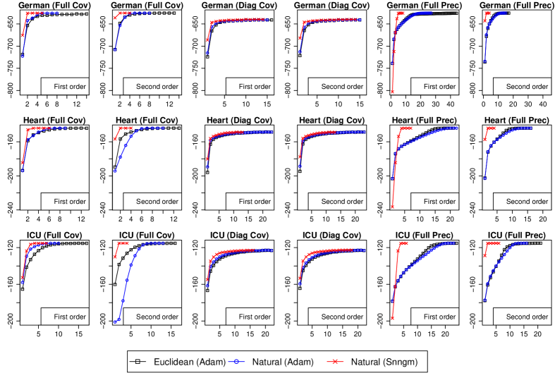
Figure 6: Logistic regression: Average lower bound attained over past 1000 iterations.

The progress of each algorithm is represented in Figure 6 through the average lower bound attained over the past 1000 iterations, while Table 7 shows the total number of iterations required (in thousands), average lower bound $\hat{{\mathcal{L}}}$ attained at termination and runtime in seconds. When the learning rate is computed using Adam, natural gradients provide some improvement relative to Euclidean gradients in terms of a higher lower bound or shorter runtime in about half of the cases. However, such improvements are much more prevalent and pronounced with Snngm. In particular, natural gradient with Snngm is often able to achieve a much higher lower bound within the first few iterations. While using natural gradients requires more computation, the improved convergence makes up for it and overall runtime can be reduced by up to a factor of 3 to 4.

The value of $\hat{{\mathcal{L}}}$ is mostly about the same across different algorithms for the same level of approximation, and $\hat{{\mathcal{L}}}$ is naturally lower for the much more restrictive diagonal covariance case. However, for the German credit data, natural gradient with Snngm is able to achieve a distinctly higher lower bound than other approaches for the full and diagonal covariance cases using first order gradient estimates. Algorithms based on second order gradient estimates often require less number of iterations to converge but the runtime is still longer due more intensive computations per iteration. First order gradient estimates are more efficient computationally, although the use of second order estimates for Algorithms 1E and 2E with Adam led to higher lower bounds than what could be achieved using first order estimates for the German credit data. Finally, while a Cholesky decomposition of the full precision instead of covariance matrix leads to similar results, computation time is increased significantly as the size of the data increases due to the matrix inversion operations that are required.

9.2 Generalized linear mixed models

Let $y_{i}=(y_{i1},\dots,y_{in_{i}})^{T}$ denote the $i$th observation for $i=1,\dots,n$. Each $y_{ij}$ is assumed to follow some distribution in the exponential family and $g({\text{E}}(y_{ij}))=\eta_{ij}$ for some link function $g(\cdot)$, where the linear predictor, $\eta_{ij}=X_{ij}^{T}\beta+Z_{ij}^{T}\theta_{i}$. Here $X_{ij}$ and $Z_{ij}$ denote covariates of length $p$ and $r$ respectively, $\beta$ denotes the fixed effects and $\theta_{i}\sim{\text{N}}(0,B^{-1})$ denote the random effects. We assume the priors, $\beta\sim{\text{N}}(0,\sigma_{\beta}^{2}I_{p})$ and $B\sim\text{W}(\nu,S)$, where $\text{W}(\nu,S)$ represents the Wishart distribution. We set $\sigma_{\beta}=10$ while $\nu$ and $S$ are determined using the default conjugate prior of Kass and Natarajan (2006). To transform all variables onto $\mathbb{R}$, consider the Cholesky decomposition $B=WW^{T}$ where $W$ is lower triangular with positive diagonal entries, and define $W^{*}$ such that $W_{ii}^{*}=\log(W_{ii})$ and $W_{ij}^{*}=W_{ij}$ if $i\neq j$. Then the joint distribution of the GLMM is of the form in Section 7.2, where $\theta_{g}=[\beta^{T},\omega^{T}]^{T}$ and $\omega=\text{vech}(W^{*})$.

We consider two variational approximations. The first is GVA (Tan and Nott, 2018), where conditional independence structure in the posterior distribution is captured using a sparse precision matrix, whose Cholesky factor $T$ is of the form in (3). Thus GVA can be found using Algorithm 2S. The second is reparametrized variational Bayes (RVB, Tan, 2021), where posterior dependence between local and global variables is first minimized by applying an invertible affine transformation on the local variables. Tan (2021) considers two transformations, which lead to the approaches RVB1 and RVB2. RVB1 is more suited to Poisson and binomial GLMMs while RVB2 works better for Bernoulli models. Let $\tilde{\theta}=(\tilde{\theta}_{1}^{T},\dots,\tilde{\theta}_{n}^{T},\theta_{g}^{T})^{T}$, where $\tilde{\theta}_{1},\dots,\tilde{\theta}_{n}$ are the transformed local variables. Variational Bayes is then applied by assuming $q(\tilde{\theta})=q(\theta_{g})\prod_{i=1}^{n}q(\tilde{\theta}_{i})$, and additionally that $q(\theta_{g})$ and each $q(\tilde{\theta}_{i})$ are Gaussian. Thus $q(\tilde{\theta})={\text{N}}(\mu,\Sigma)$ where $\Sigma$ is a block diagonal matrix with $n+1$ blocks. If we consider a Cholesky decomposition $CC^{T}=\Sigma$, then RVB1 and RVB2 can be obtained using Algorithm 1S. In RVB, the local variables are transformed to be approximately Gaussian with mean 0 and variance 1. Hence, we initialize $C$ as a diagonal matrix where diagonal elements corresponding to local variables and global variables are set at 1 and 0.1 respectively.

We study three benchmark datasets analyzed in Tan (2021). The first is the Epilepsy data (Thall and Vail, 1990), where $n=59$ epileptics are randomly assigned a new drug Progabide or a placebo, and $y_{ij}$ is the number of seizures of patient $i$ in the two weeks before clinic visit $j$ for $j=1,\dots,4$. Consider the Poisson random slope model,

$$\log\mu_{ij}=\beta_{1}+\beta_{2}\text{Base}_{i}+\beta_{3}\text{Trt}_{i}+\beta_{4}\text{Base}_{i}\times\text{Trt}_{i}+\beta_{5}\text{Age}_{i}+\beta_{6}\text{Visit}_{ij}+b_{i1}+b_{i2}\text{Visit}_{ij},$$

where the covariates for patient $i$ are $\text{Base}_{i}$ (log(number of baseline seizures/4)), $\text{Trt}_{i}$ (1 for drug and 0 for placebo), $\text{Age}_{i}$ (log(age of patient at baseline) centered at zero) and $\text{Visit}_{ij}$ (coded as $-0.3$, $-0.1$, $0.1$, $0.3$ for $j=1,\dots,4$). For the prior hyperparameters, $\nu=3$, $S_{11}=11.0169$, $S_{12}=-0.1616$ and $S_{22}=0.5516$.

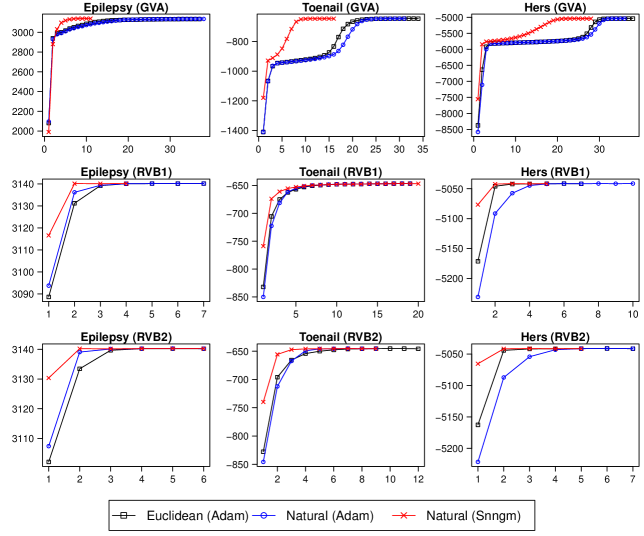
Figure 7: GLMMs: Average lower bound attained over past 1000 iterations.

Table 8: GLMMs: Number of iterations ($T$) in thousands that each algorithm was run, average lower bound $\hat{{\mathcal{L}}}$ attained at termination and runtime in seconds.

Epilepsy Toenail Hers $T$ $\hat{{\mathcal{L}}}$ time $T$ $\hat{{\mathcal{L}}}$ time $T$ $\hat{{\mathcal{L}}}$ time GVA Euclidean (Adam) 37 3135.1 11.0 34 -646.2 17.0 38 -5042.2 130.1 Natural (Adam) 38 3136.0 17.0 31 -646.3 21.2 36 -5042.3 165.5 Natural (Snngm) 11 3139.4 4.4 16 -646.4 9.8 28 -5041.8 118.9 RVB1 Euclidean (Adam) 7 3140.1 2.2 19 -646.7 7.2 7 -5041.3 15.4 Natural (Adam) 7 3140.1 2.5 19 -646.7 8.2 10 -5041.3 26.0 Natural (Snngm) 4 3140.1 1.4 20 -646.7 8.4 5 -5041.3 12.9 RVB2 Euclidean (Adam) 6 3140.2 4.5 12 -645.6 25.5 7 -5041.0 67.5 Natural (Adam) 6 3140.2 4.7 9 -645.6 19.3 7 -5041.0 68.5 Natural (Snngm) 6 3140.2 4.6 9 -645.6 19.7 5 -5041.0 49.3

The second is the Toenail data (De Backer et al., 1998), where two treatments for toenail infection are compared for $n=294$ patients. The binary response $y_{ij}$ of patient $i$ at the $j$th visit is 1 if degree of separation of nail plate from nail bed is moderate or severe and 0 if none or mild. Consider the random intercept model,

$$\text{logit}(p_{ij})=\beta_{1}+\beta_{2}\text{Trt}_{i}+\beta_{3}t_{ij}+\beta_{4}\text{Trt}_{i}\times t_{ij}+\theta_{i},\quad 1\leq j\leq 7,$$

where for the $i$th patient, $\text{Trt}_{i}=1$ if 250mg of terbinafine is taken each day and 0 if 200mg of itraconazole is taken, and $t_{ij}$ is the time in months when the patient is evaluated at the $j$th visit. The prior for $B$ is Gamma(0.5, 0.4962).

The third dataset which is available at www.biostat.ucsf.edu/vgsm/data.html comes from the Heart and Estrogen/Progestin Study (HERS, Hulley et al., 1998). We examine 2031 women whose data for all covariates are available. The binary response $y_{ij}$ of patient $i$ at the $j$th visit indicates whether the systolic blood pressure is above 140. Consider the random intercept model,

$$\text{logit}(p_{ij}) =\beta_{1}+\beta_{2}\text{age}_{i}+\beta_{3}\text{BMI}_{ij}+\beta_{4}\text{HTN}_{ij}+\beta_{5}\text{visit}_{ij}+\theta_{i},\quad 0\leq j\leq 5,$$

where for patient $i$, $\text{age}_{i}$ is the age at baseline, $\text{BMI}_{ij}$ is the body mass index at the $j$th visit, $\text{HTN}_{ij}$ indicates whether high blood pressure medication is taken at the $j$th visit and $\text{visit}_{ij}$ is coded as $-1$, $-0.6$, $-0.2$, 0.2, 0.6, 1 for $j=0,1,\dots,5$ respectively. We normalize BMI and age to have mean 0 and standard deviation 1 and the prior for $B$ is Gamma(0.5, 0.5079).

Figure 7 shows the average lower bounds attained over the past 1000 iterations for each algorithm and dataset, while Table 8 shows the total number of iterations, average lower bound attained and runtime. These results are based on first order gradient estimates as $\nabla_{\theta}^{2}h(\theta)$ is highly complex for GVA and RVB and it is unlikely that second order gradient estimates will be more efficient than first order ones. The use of natural gradients with Adam did not bring about significant improvement in convergence relative to Euclidean gradients. In almost all cases, about the same number of iterations is required. However, natural gradients with Snngm yields much better results and runtime can be improved by up to a factor of 2.5 in the case of GVA for the Epilepsy data (together with a distinctly higher lower bound).

Figure 7 also shows that natural gradients with Snngm seem to be able to escape suboptimal local modes more effectively in the case of GVA for the Toenail and Hers datasets. Generally, GVA takes much more iterations to converge than RVB because the local variables in RVB are transformed so that they are approximately distributed as standard normals a posteriori. Hence, by initializing their mean as 0 and variance as 1, the algorithm is already closer to convergence. While RVB1 is the fastest to converge, RVB2 yields the highest lower bound. All three approaches are able to benefit from the use of natural gradients with Snngm, with GVA seeing the biggest reduction in number of iterations required.

10 Conclusion

Gaussian variational approximation is widely used and natural gradients provide a direct means of improving the convergence in stochastic gradient ascent, which is particularly important when suboptimal local modes are present. However, the natural gradient update of the precision matrix does not ensure positive definiteness. To tackle this issue, we consider Cholesky decomposition of the covariance or precision matrix. We show that the inverse Fisher information can be found analytically and present natural gradient updates of the Cholesky factors in closed form. We also derive unbiased gradient estimates in terms of the first or second derivative of the log posterior when the gradient of the lower bound is not available analytically. While second order gradient estimates are more stable and can lead to more accurate variational approximations, they require intensive computations and first order gradient estimates are still more efficient in most cases. For high-dimensional models, we impose sparsity constraints on the covariance or precision matrix to incorporate assumptions in variational Bayes or conditional independence structure in the posterior, and we show that efficient natural gradient updates can also be derived in these cases. Finally, we observe that Adam does not always perform well with natural gradients and we propose stochastic normalized natural gradient ascent with momentum (Snngm) as an alternative. We prove the convergence of this approach for $L$-Lipschitz smooth functions with bounded gradients and demonstrate its efficiency in logistic regression and GLMMs for several real datasets.

Supplementary material

S1 Natural gradient updates in terms of mean and covariance/precision matrix

First we derive the natural gradient of ${\mathcal{L}}$ with respect to the natural parameter $\lambda$ using $\widetilde{\nabla}_{\lambda}{\mathcal{L}}=\nabla_{m}{\mathcal{L}}$. For the Gaussian, $m={\text{E}}[s(\theta)]=(m_{1}^{T},m_{2}^{T})^{T}$, where $m_{1}=\mu$, $m_{2}=\text{vech}(\Sigma+\mu\mu^{T})$. We introduce $\zeta=(\zeta_{1}^{T},\zeta_{2}^{T})^{T}$, where

$$\zeta_{1}=\mu=m_{1},\quad\zeta_{2}=\text{vech}(\Sigma)=m_{2}-\text{vech}(m_{1}m_{1}^{T}).$$

Then

$$\nabla_{m}\zeta=\begin{bmatrix}I_{d}&-2(I_{d}\otimes\mu^{T}){D^{+}}^{T}\\ 0_{d(d+1)/2\times d}&I_{d(d+1)/2}\end{bmatrix}.$$

Applying chain rule, the natural gradient is

$$\widetilde{\nabla}_{\lambda}{\mathcal{L}} =\nabla_{m}{\mathcal{L}}=\nabla_{m}\zeta\nabla_{\zeta}{\mathcal{L}}$$

$$=\begin{bmatrix}I_{d}&-2(I_{d}\otimes\mu^{T}){D^{+}}^{T}\\ 0_{d(d+1)/2\times d}&I_{d(d+1)/2}\end{bmatrix}\begin{bmatrix}\nabla_{\mu}{\mathcal{L}}\\ \nabla_{\text{vech}(\Sigma)}{\mathcal{L}}\end{bmatrix}$$

$$=\begin{bmatrix}\nabla_{\mu}{\mathcal{L}}-2(I_{d}\otimes\mu^{T})\text{vec}(\nabla_{\Sigma}{\mathcal{L}})\\ D^{T}\text{vec}(\nabla_{\Sigma}{\mathcal{L}})\end{bmatrix}$$

$$=\begin{bmatrix}\nabla_{\mu}{\mathcal{L}}-2(\nabla_{\Sigma}{\mathcal{L}})\mu\\ D^{T}\text{vec}(\nabla_{\Sigma}{\mathcal{L}})\end{bmatrix}.$$

Next, consider the parametrization, $\kappa=(\mu^{T},\text{vech}(\Sigma)^{T})^{T}$. The Fisher information matrix and its inverse are respectively,

$$F_{\kappa}=\begin{bmatrix}\Sigma^{-1}&0\\ 0&\frac{1}{2}D^{T}(\Sigma^{-1}\otimes\Sigma^{-1})D\end{bmatrix},\quad F_{\kappa}^{-1}=\begin{bmatrix}\Sigma&0\\ 0&2D^{+}(\Sigma\otimes\Sigma){D^{+}}^{T}\end{bmatrix}.$$

Hence the natural gradient is

$$\widetilde{\nabla}_{\kappa}{\mathcal{L}}=\begin{bmatrix}\Sigma&0\\ 0&2D^{+}(\Sigma\otimes\Sigma){D^{+}}^{T}\end{bmatrix}\begin{bmatrix}\nabla_{\mu}{\mathcal{L}}\\ \nabla_{\text{vech}(\Sigma)}{\mathcal{L}}\end{bmatrix}=\begin{bmatrix}\Sigma\nabla_{\mu}{\mathcal{L}}\\ 2\text{vech}(\Sigma\nabla_{\Sigma}{\mathcal{L}}\Sigma)\end{bmatrix}.$$

Alternatively, $\widetilde{\nabla}_{\kappa}{\mathcal{L}}=(\nabla_{\lambda}\kappa)^{T}\widetilde{\nabla}_{\lambda}{\mathcal{L}}$, which is equal to

$$\begin{bmatrix}\Sigma&-\Sigma(\mu^{T}\Sigma^{-1}\otimes\Sigma^{-1})DD^{+}(\Sigma\otimes\Sigma){D^{+}}^{T}\\ 0&-D^{+}(\Sigma\otimes\Sigma){D^{+}}^{T}\end{bmatrix}\begin{bmatrix}\nabla_{\mu}{\mathcal{L}}-2(\nabla_{\Sigma}{\mathcal{L}})\mu\\ -2D^{T}\text{vec}(\nabla_{\Sigma}{\mathcal{L}})\end{bmatrix}=\begin{bmatrix}\Sigma\nabla_{\mu}{\mathcal{L}}\\ 2\text{vech}(\Sigma\nabla_{\Sigma}{\mathcal{L}}\Sigma)\end{bmatrix}.$$

For the parametrization $\xi=(\mu^{T},\text{vech}(\Sigma^{-1})^{T})^{T}$, the Fisher information and its inverse are respectively,

$$F_{\xi}=\begin{bmatrix}\Sigma^{-1}&0\\ 0&\frac{1}{2}D^{T}(\Sigma\otimes\Sigma)D\end{bmatrix},\quad F_{\xi}^{-1}=\begin{bmatrix}\Sigma&0\\ 0&2D^{+}(\Sigma^{-1}\otimes\Sigma^{-1}){D^{+}}^{T}\end{bmatrix}.$$

Hence the natural gradient is

$$\widetilde{\nabla}_{\xi}{\mathcal{L}}=\begin{bmatrix}\Sigma&0\\ 0&2D^{+}(\Sigma^{-1}\otimes\Sigma^{-1}){D^{+}}^{T}\end{bmatrix}\begin{bmatrix}\nabla_{\mu}{\mathcal{L}}\\ \nabla_{\text{vech}(\Sigma)}{\mathcal{L}}\end{bmatrix}=\begin{bmatrix}\Sigma\nabla_{\mu}{\mathcal{L}}\\ -2\text{vech}(\nabla_{\Sigma}{\mathcal{L}})\end{bmatrix},$$

Alternatively, $\widetilde{\nabla}_{\xi}{\mathcal{L}}=(\nabla_{\lambda}\xi)^{T}\widetilde{\nabla}_{\lambda}{\mathcal{L}}$, which is equal to

$$=\begin{bmatrix}\Sigma&-\Sigma(\mu^{T}\otimes I){D^{+}}^{T}\\ 0&(D^{T}D)^{-1}\end{bmatrix}\begin{bmatrix}\nabla_{\mu}{\mathcal{L}}-2(\nabla_{\Sigma}{\mathcal{L}})\mu\\ -2D^{T}\text{vec}(\nabla_{\Sigma}{\mathcal{L}})\end{bmatrix}=\begin{bmatrix}\Sigma\nabla_{\mu}{\mathcal{L}}\\ -2\text{vech}(\nabla_{\Sigma}{\mathcal{L}})\end{bmatrix}.$$

S2 Loglinear model for Poisson counts

Let $y=(y_{1},\dots,y_{n})^{T}$ an $X=(x_{1},\dots,x_{n})^{T}$. We have $\log\delta_{i}=x_{i}^{T}\theta$ and $\delta_{i}=\exp(x_{i}^{T}\theta)$ for $i=1,\dots,n$. The lower bound can be evaluated analytically and it is given by

$${\mathcal{L}}(\lambda) ={\text{E}}_{q}\{\log p(y,\theta)-\log q_{\lambda}(\theta)\}$$

$$={\text{E}}_{q}\bigg{[}y^{T}X\theta-\sum_{i=1}^{n}\{\exp(x_{i}^{T}\theta)+\log(y_{i}!)\}-\frac{d}{2}\log(2\pi)-\frac{d}{2}\log(\sigma_{0}^{2})-\frac{\theta^{T}\theta}{2\sigma_{0}^{2}}\bigg{]}$$

$$\quad-{\text{E}}_{q}\bigg{[}-\frac{d}{2}\log(2\pi)-\frac{1}{2}\log|\Sigma|-\frac{1}{2}(\theta-\mu)^{T}\Sigma^{-1}(\theta-\mu)\bigg{]}$$

$$=y^{T}X\mu-\sum_{i=1}^{n}\{w_{i}+\log(y_{i}!)\}-\frac{\mu^{T}\mu+\text{tr}(\Sigma)}{2\sigma_{0}^{2}}+\frac{1}{2}\log|\Sigma|+\frac{d}{2}\{1-\log(\sigma_{0}^{2})\},$$

where $w_{i}=\exp(x_{i}^{T}\mu+\frac{1}{2}x_{i}^{T}\Sigma x_{i})$. Let $w=(w_{1},\dots,w_{n})^{T}$ and $W={\text{diag}}(w)$. Then the Euclidean gradients are given by

$$\nabla_{\mu}{\mathcal{L}} =X^{T}(y-w)-\mu/\sigma_{0}^{2},\quad\nabla_{\text{vec}(\Sigma)}{\mathcal{L}}=\tfrac{1}{2}\text{vec}(\Sigma^{-1}-I/\sigma_{0}^{2}-X^{T}WX)$$

$$\nabla_{\text{vech}(T)} =\text{vech}(\{\Sigma X^{T}WX+\Sigma/\sigma_{0}^{2}-I\}T^{-T}).$$

S3 Natural gradient updates in terms of mean and Cholesky factor

First we present the proof of Lemma 1. As this proof requires several results from Magnus and Neudecker (1980) concerning the elimination matrix $L$, these are collected here in Lemma S1 for ease of reference.

Lemma S1

If $P$ and $Q$ are lower triangular $d\times d$ matrices and $N=(I+K)/2$, then

1. $LL^{T}=I_{d(d+1)/2}$,

2. $(LNL^{T})^{-1}=2I_{d(d+1)/2}-LKL^{T}$,

3. $N=DLN$,

4. $L^{T}L(P^{T}\otimes Q)L^{T}=(P^{T}\otimes Q)L^{T}$ and its transpose, $L(P\otimes Q^{T})L^{T}L=L(P\otimes Q^{T})$,

5. $L(P^{T}\otimes Q)L^{T}=D^{T}(P^{T}\otimes Q)L^{T}$ and its transpose, $L(P\otimes Q^{T})L^{T}=L(P\otimes Q^{T})D$.

Proof S3.4 (Lemma S1).

The proofs can be found in Lemma 3.2 (ii), Lemma 3.4 (ii), Lemma 3.5 (ii) and Lemma 4.2 (i) and (iii) of Magnus and Neudecker (1980) respectively.

S3.1 Proof of Lemma 1

First, we prove (i):

$$\mathfrak{I}(\Lambda) =L\{K(\Lambda^{-T}\otimes\Lambda^{-1})+I_{d}\otimes\Lambda^{-T}\Lambda^{-1}\}L^{T}$$

$$=L\{K(\Lambda^{-T}\otimes I_{d})(I_{d}\otimes\Lambda^{-1})+(I_{d}\otimes\Lambda^{-T})(I_{d}\otimes\Lambda^{-1})\}L^{T}$$

$$=L\{(I_{d}\otimes\Lambda^{-T})K+(I_{d}\otimes\Lambda^{-T})\}(I_{d}\otimes\Lambda^{-1})L^{T}$$

$$=L(I_{d}\otimes\Lambda^{-T})(K+I_{d^{2}})(I_{d}\otimes\Lambda^{-1})L^{T}$$

$$=2L(I_{d}\otimes\Lambda^{-T})N(I_{d}\otimes\Lambda^{-1})L^{T}.$$

Next we prove (ii) and (iii) by using the results in Lemma S1. The roman letters in square brackets on the right indicate which parts of Lemma S1 are used. For (ii),

$$\{2L(I_{d}\otimes\Lambda^{-T})N(I_{d}\otimes\Lambda^{-1})L^{T}\}\left\{\tfrac{1}{2}L(I_{d}\otimes\Lambda)L^{T}(LNL^{T})^{-1}L(I_{d}\otimes\Lambda^{T})L^{T}\right\}$$

$$=L(I_{d}\otimes\Lambda^{-T})(DLN)(I_{d}\otimes\Lambda^{-1})(I_{d}\otimes\Lambda)L^{T}(LNL^{T})^{-1}L(I_{d}\otimes\Lambda^{T})L^{T}$$ [(iii) & (iv)]

$$=L(I_{d}\otimes\Lambda^{-T})L^{T}(LNL^{T})(LNL^{T})^{-1}L(I_{d}\otimes\Lambda^{T})L^{T}$$ [(v)]

$$=L(I_{d}\otimes\Lambda^{-T})L^{T}L(I_{d}\otimes\Lambda^{T})L^{T}$$

$$=L(I_{d}\otimes\Lambda^{-T})(I_{d}\otimes\Lambda^{T})L^{T}$$ [(iv)]

$$=LL^{T}=I_{d(d+1)/2}.$$ [(i)]

For (iii),

$$\mathfrak{I}(\Lambda)^{-1}\text{vech}(G) =\tfrac{1}{2}L(I_{d}\otimes\Lambda)L^{T}(LNL^{T})^{-1}L(I_{d}\otimes\Lambda^{T})L^{T}\text{vech}(\bar{G})$$

$$=\tfrac{1}{2}L(I_{d}\otimes\Lambda)L^{T}(2I_{d(d+1)/2}-LKL^{T})L(I_{d}\otimes\Lambda^{T})\text{vec}(\bar{G})$$ [(ii)]

$$=\tfrac{1}{2}L(I_{d}\otimes\Lambda)(2I_{d^{2}}-L^{T}LK)L^{T}L\text{vec}(\Lambda^{T}\bar{G})$$

$$=\tfrac{1}{2}L(I_{d}\otimes\Lambda)(2I_{d^{2}}-L^{T}LK)L^{T}\text{vech}(\bar{H})$$

$$=\tfrac{1}{2}L(I_{d}\otimes\Lambda)(2I_{d^{2}}-L^{T}LK)\text{vec}(\bar{H})$$

$$=L(I_{d}\otimes\Lambda)\text{vec}(\bar{H})-\tfrac{1}{2}L(I_{d}\otimes\Lambda)L^{T}LK\text{vec}(\bar{H})$$

$$=L\text{vec}(\Lambda\bar{H})-\tfrac{1}{2}L(I_{d}\otimes\Lambda)L^{T}\text{vech}(\bar{H}^{T})$$

$$=\text{vech}(\Lambda\bar{H})-\tfrac{1}{2}L(I_{d}\otimes\Lambda)\text{vec}({\text{dg}}(\bar{H}))$$

$$=\text{vech}(\Lambda\bar{H})-\tfrac{1}{2}\text{vech}(\Lambda{\text{dg}}(\bar{H}))=\text{vech}(\Lambda\bar{\bar{H}}).$$

S3.2 Proof of Theorem 1

First we derive the Fisher information and its inverse for each of the two parametrizations. We have

$$\ell_{q}=\log q_{\lambda}(\theta)=-\tfrac{d}{2}\log(2\pi)-\tfrac{1}{2}\log|\Sigma|-\tfrac{1}{2}(\theta-\mu)^{T}\Sigma^{-1}(\theta-\mu).$$

For the first parametrization, $\lambda=(\mu^{T},\text{vech}(C)^{T})^{T}$, let $z=C^{-1}(\theta-\mu)$ to simplify expressions. The first order derivatives are

$$\nabla_{\mu}\ell_{q}=\Sigma^{-1}(\theta-\mu),\quad\nabla_{\text{vech}(C)}\ell_{q}=\text{vech}(C^{-T}zz^{T}-C^{-T}),$$

and $-\nabla_{\lambda}^{2}\ell_{q}$ is given by

$$\begin{bmatrix}\Sigma^{-1}&\{(C^{-T}\otimes z^{T}C^{-1})+(z^{T}\otimes\Sigma^{-1})\}L^{T}\\ \cdot&L[\{(C^{-1}\otimes C^{-T}zz^{T})+(zz^{T}C^{-1}\otimes C^{-T})-(C^{-1}\otimes C^{-T})\}K+zz^{T}\otimes\Sigma^{-1}]L^{T}\end{bmatrix}.$$

Taking the negative expectation of $\nabla_{\lambda}^{2}\ell_{q}$ and applying the fact that ${\text{E}}(z)=0$ and ${\text{E}}(zz^{T})=I_{d}$, we obtain

$$F_{\lambda}=\begin{bmatrix}\Sigma^{-1}&0\\ 0&L\{(C^{-1}\otimes C^{-T})K+(I_{d}\otimes\Sigma^{-1})\}L^{T}\end{bmatrix}=\begin{bmatrix}\Sigma^{-1}&0\\ 0&\mathfrak{I}(C)\end{bmatrix}.$$

Thus $F_{\lambda}^{-1}={\text{blockdiag}}(\Sigma,\mathfrak{I}(C)^{-1})$.

For the second parametrization, $\lambda=(\mu^{T},\text{vech}(T)^{T})^{T}$, the first order derivative,

$$\nabla_{\text{vech}(T)}\ell_{q}=\text{vech}(T^{-T}-(\theta-\mu)(\theta-\mu)^{T}T)$$

and

$$\nabla_{\lambda}^{2}\ell_{q}=-\begin{bmatrix}\Sigma^{-1}&-\{(\theta-\mu)^{T}T\otimes I_{d}+T\otimes(\theta-\mu)^{T}\}L^{T}\\ \cdot&L\{(T^{-1}\otimes T^{-T})K+I_{d}\otimes(\theta-\mu)(\theta-\mu)^{T}\}L^{T}\end{bmatrix}.$$

Taking the negative expectation of $\nabla_{\lambda}^{2}\ell_{q}$ and applying the fact that ${\text{E}}(\theta)=\mu$ and ${\text{E}}[(\theta-\mu)(\theta-\mu)^{T}]=\Sigma$, we obtain

$$F_{\lambda}=\begin{bmatrix}\Sigma^{-1}&0\\ 0&L\{(T^{-1}\otimes T^{-T})K+I_{d}\otimes\Sigma\}L^{T}\end{bmatrix}=\begin{bmatrix}\Sigma^{-1}&0\\ 0&\mathfrak{I}(T)\end{bmatrix}.$$

Thus $F_{\lambda}^{-1}={\text{blockdiag}}(\Sigma,\mathfrak{I}(T)^{-1})$.

Suppose $\nabla_{\text{vech}(\Lambda)}{\mathcal{L}}=\text{vech}(G)$. Then, for each parametrization, the natural gradient is

$$\widetilde{\nabla}_{\lambda}{\mathcal{L}}=F_{\lambda}^{-1}\nabla_{\lambda}{\mathcal{L}}=\begin{bmatrix}\Sigma&0\\ 0&\mathfrak{I}(\Lambda)^{-1}\end{bmatrix}\begin{bmatrix}\nabla_{\mu}{\mathcal{L}}\\ \text{vech}(G)\end{bmatrix}=\begin{bmatrix}\Sigma\nabla_{\mu}{\mathcal{L}}\\ \text{vech}(\Lambda\bar{\bar{H}})\end{bmatrix},$$

where we have applied Lemma 1 (iii) in the last step.

S3.3 Proof of Corollary 1

If $\xi=((T^{T}\mu)^{T},\text{vech}(T)^{T})^{T}$, then

$$\widetilde{\nabla}_{\xi}{\mathcal{L}}=(\nabla_{\lambda}\xi)^{T}\widetilde{\nabla}_{\lambda}{\mathcal{L}}=\begin{bmatrix}T^{T}&(I\otimes\mu^{T})L^{T}\\ 0&I\end{bmatrix}\begin{bmatrix}\Sigma\nabla_{\mu}{\mathcal{L}}\\ \text{vech}(T\bar{\bar{H}})\end{bmatrix}=\begin{bmatrix}T^{-1}\nabla_{\mu}{\mathcal{L}}+\bar{\bar{H}}^{T}T^{T}\mu\\ \text{vech}(T\bar{\bar{H}})\end{bmatrix}.$$

The natural gradient ascent update is

$$T^{(t+1)T}\mu^{(t+1)} =T^{(t)T}\mu^{(t)}+\rho_{t}\{T^{(t)-1}\nabla_{\mu}{\mathcal{L}}+\bar{\bar{H}}^{(t)T}T^{(t)T}\mu^{(t)}\},$$

$$T^{(t+1)} =T^{(t)}+\rho_{t}T^{(t)}\bar{\bar{H}}^{(t)},$$

The first line simplifies to

$$T^{(t+1)T}\mu^{(t+1)} =\{T^{(t)}+\rho_{t}T^{(t)}\bar{\bar{H}}^{(t)}\}^{T}\mu^{(t)}+\rho_{t}T^{(t)-1}\nabla_{\mu}{\mathcal{L}}$$

$$\implies\mu^{(t+1)} =\mu^{(t)}+\rho_{t}T^{-(t+1)T}T^{(t)-1}\nabla_{\mu}{\mathcal{L}}.$$

S3.4 Proof of Lemma 2

Define $g(\theta)=(\theta-\mu)^{T}e_{j}h(\theta)$ to be a function from $\mathbbm{R}^{d}$ to $\mathbbm{R}$ and $e_{j}$ to be a $d\times 1$ vector with the $j$th element equal to one and zero elsewhere. Then

$$\nabla_{\theta}g(\theta)=h(\theta)e_{j}+(\theta-\mu)^{T}e_{j}\nabla_{\theta}h(\theta).$$

Replacing $f(\theta)$ by $g(\theta)$ in Stein’s Lemma, we obtain

$${\text{E}}_{q}[\Sigma^{-1}(\theta-\mu)(\theta-\mu)^{T}e_{j}h(\theta)]={\text{E}}_{q}[h(\theta)e_{j}+(\theta-\mu)^{T}e_{j}\nabla_{\theta}h(\theta)].$$

This implies that for any $1\leq i,j\leq d$,

$$e_{i}^{T}{\text{E}}_{q}[\{\Sigma^{-1}(\theta-\mu)(\theta-\mu)^{T}-I_{d}\}h(\theta)]e_{j}=e_{i}^{T}{\text{E}}_{q}[\nabla_{\theta}h(\theta)(\theta-\mu)^{T}]e_{j}.$$

Thus ${\text{E}}_{q}[\{\Sigma^{-1}(\theta-\mu)(\theta-\mu)^{T}-I_{d}\}h(\theta)]={\text{E}}_{q}[\nabla_{\theta}h(\theta)(\theta-\mu)^{T}]$ since every $(i,j)$ element of these two matrices agree with each other.

S3.5 Proof of Theorem 2

First we prove (i) of Theorem 2. Post-multiplying the identity in Lemma 2 by $C^{-T}$, we obtain

$${\text{E}}_{q}[\{\Sigma^{-1}(\theta-\mu)(\theta-\mu)^{T}C^{-T}-C^{-T}\}h(\theta)]={\text{E}}_{q}[\nabla_{\theta}h(\theta)(\theta-\mu)^{T}C^{-T}]={\text{E}}_{q}({\mathcal{G}}_{1}).$$

Hence

$$\nabla_{\text{vech}(C)}{\mathcal{L}} =\int\nabla_{\text{vech}(C)}q_{\lambda}(\theta)h(\theta){\text{d}}\theta$$

$$=\int q_{\lambda}(\theta)\text{vech}\left\{\Sigma^{-1}(\theta-\mu)(\theta-\mu)^{T}C^{-T}-C^{-T}\right\}h(\theta){\text{d}}\theta$$

$$={\text{E}}_{q}\left[\text{vech}\{\Sigma^{-1}(\theta-\mu)(\theta-\mu)^{T}C^{-T}-C^{-T}\}h(\theta)\right]={\text{E}}_{q}\text{vech}({\mathcal{G}}_{1}),$$

and the first part of the identity in Theorem 2 (i) is shown. For the second part of the identity, we have ${\text{E}}_{q}[\Sigma^{-1}(\theta-\mu)\nabla_{\theta}h(\theta)^{T}]={\text{E}}_{q}[\nabla_{\theta}^{2}h(\theta)]$ from Price’s Theorem. Taking the transpose and post-multiplying by $C$, we obtain

$${\text{E}}_{q}({\mathcal{G}}_{1})={\text{E}}_{q}[\nabla_{\theta}h(\theta)(\theta-\mu)^{T}C^{-T}]={\text{E}}_{q}[\nabla_{\theta}^{2}h(\theta)C]={\text{E}}_{q}({\mathcal{F}}_{1}).$$

Next, First we prove (ii) of Theorem 2. Taking the transpose of the identity in Lemma 2 and post-multiplying by $T^{-T}$,

$${\text{E}}_{q}[\{(\theta-\mu)(\theta-\mu)^{T}T-T^{-T}\}h(\theta)]={\text{E}}_{q}[(\theta-\mu)\nabla_{\theta}h(\theta)^{T}T^{-T}]=-{\text{E}}_{q}({\mathcal{G}}_{2}).$$

Hence

$$\nabla_{\text{vech}(T)}{\mathcal{L}} =\int\nabla_{\text{vech}(T)}q_{\lambda}(\theta)h(\theta){\text{d}}\theta$$

$$=\int q_{\lambda}(\theta)\text{vech}\{T^{-T}-(\theta-\mu)(\theta-\mu)^{T}T\}h(\theta){\text{d}}\theta$$

$$={\text{E}}_{q}[\text{vech}\{T^{-T}-(\theta-\mu)(\theta-\mu)^{T}T\}h(\theta)]={\text{E}}_{q}\text{vech}({\mathcal{G}}_{2}),$$

and the first part of the identity in Theorem 2 (ii) is shown. For the second part of the identity, we have ${\text{E}}_{q}[\Sigma^{-1}(\theta-\mu)\nabla_{\theta}h(\theta)^{T}]={\text{E}}_{q}[\nabla_{\theta}^{2}h(\theta)]$ from Price’s Theorem. Pre-multiplying by $\Sigma$ and post-multiplying by $T^{-T}$, we obtain

$$-{\text{E}}_{q}({\mathcal{G}}_{2})={\text{E}}_{q}[(\theta-\mu)\nabla_{\theta}h(\theta)^{T}T^{-T}]={\text{E}}_{q}[\Sigma\nabla_{\theta}^{2}h(\theta)T^{-T}]=-{\text{E}}_{q}({\mathcal{F}}_{2}).$$

S4 Natural gradient for sparse precision matrix

We derive the natural gradient where the precision matrix is sparse. In this case,

$$\ell_{q} =\log q_{\lambda}(\theta)=-\frac{d}{2}\log(2\pi)+\log|T_{g}|+\sum_{i=1}^{N}\log|T_{i}|-\frac{1}{2}\sum_{i=1}^{n}(\theta_{i}-\mu_{i})^{T}T_{i}T_{i}^{T}(\theta_{i}-\mu_{i})$$

$$-\frac{1}{2}(\theta_{g}-\mu_{g})^{T}\left(\sum_{i=1}^{n}T_{gi}T_{g_{i}}^{T}+T_{g}T_{g}^{T}\right)(\theta_{g}-\mu_{g})-(\theta_{g}-\mu_{g})^{T}\sum_{i=1}^{n}T_{gi}T_{i}^{T}(\theta_{i}-\mu_{i}).$$

In addition, if we integrate out all other variables from $q_{\lambda}(\theta)=\prod_{i=1}^{n}q(\theta_{i}|\theta_{g})q(\theta_{g})$ except $\theta_{i}$ and $\theta_{g}$, then we have $q(\theta_{i},\theta_{g})=q(\theta_{i}|\theta_{g})q(\theta_{g})$, whose covariance matrix is

$$\begin{bmatrix}T_{i}&0\\ T_{gi}&T_{g}\end{bmatrix}^{-T} \begin{bmatrix}T_{i}&0\\ T_{gi}&T_{g}\end{bmatrix}^{-1}=\begin{bmatrix}T_{i}^{-T}&-T_{i}^{-T}T_{gi}^{T}T_{g}^{-T}\\ 0&T_{g}^{-T}\end{bmatrix}\begin{bmatrix}T_{i}^{-1}&0\\ -T_{g}^{-1}T_{gi}T_{i}^{-1}&T_{g}^{-1}\end{bmatrix}$$

$$=\begin{bmatrix}T_{i}^{-T}T_{i}^{-1}+T_{i}^{-T}T_{gi}^{T}T_{g}^{-T}T_{g}^{-1}T_{gi}T_{i}^{-1}&-T_{i}^{-T}T_{gi}^{T}T_{g}^{-T}T_{g}^{-1}\\[2.84526pt] -T_{g}^{-T}T_{g}^{-1}T_{gi}T_{i}^{-1}&T_{g}^{-T}T_{g}^{-1}\end{bmatrix}.$$

Hence ${\text{Cov}}(\theta_{g})={\text{E}}\{(\theta_{g}-\mu_{g})(\theta_{g}-\mu_{g})^{T}\}=T_{g}^{-T}T_{g}^{-1}$,

$${\text{Cov}}(\theta_{i}) ={\text{E}}\{(\theta_{i}-\mu_{i})(\theta_{i}-\mu_{i})^{T}\}=T_{i}^{-T}T_{i}^{-1}+T_{i}^{-T}T_{gi}^{T}T_{g}^{-T}T_{g}^{-1}T_{gi}T_{i}^{-1},$$

$${\text{Cov}}(\theta_{i},\theta_{g}) ={\text{E}}\{(\theta_{i}-\mu_{i})(\theta_{g}-\mu_{g})^{T}\}=-T_{i}^{-T}T_{gi}^{T}T_{g}^{-T}T_{g}^{-1}.$$

First, we find the elements in the Fisher information matrix. Differentiating $\ell_{q}$ with respect to $T_{i}$ and taking expectation with respect to $q_{\lambda}(\theta)$,

$$\nabla_{\text{vech}(T_{i})}\ell_{q} =\text{vech}\{T_{i}^{-T}-(\theta_{i}-\mu_{i})(\theta_{i}-\mu_{i})^{T}T_{i}-(\theta_{i}-\mu_{i})(\theta_{g}-\mu_{g})^{T}T_{gi}\},$$

$$\nabla_{\text{vech}(T_{i})}^{2}\ell_{q} =-L\{(T_{i}^{-1}\otimes T_{i}^{-T})K+I\otimes(\theta_{i}-\mu_{i})(\theta_{i}-\mu_{i})^{T}\}L^{T},$$

$${\text{E}}[\nabla_{\text{vech}(T_{i})}^{2}\ell_{q}] =-L\{(T_{i}^{-1}\otimes T_{i}^{-T})K+I\otimes T_{i}^{-T}(I+T_{gi}^{T}T_{g}^{-T}T_{g}^{-1}T_{gi})T_{i}^{-1}\}L^{T}$$

$$=-\mathfrak{I}(T_{i})-L(I\otimes T_{i}^{-T}T_{gi}^{T}T_{g}^{-T}T_{g}^{-1}T_{gi}T_{i}^{-1})L^{T}.$$

Differentiating $\nabla_{\text{vech}(T_{i})}\ell_{q}$ with respect to $T_{gi}$ and taking expectation with respect to $q_{\lambda}(\theta)$,

$$\nabla_{\text{vech}(T_{i}),\text{vec}(T_{gi})}^{2}\ell_{q} =-L\{I\otimes(\theta_{i}-\mu_{i})(\theta_{g}-\mu_{g})^{T}\},$$

$${\text{E}}[\nabla_{\text{vech}(T_{i}),\text{vec}(T_{gi})}^{2}\ell_{q}] =L(I\otimes T_{i}^{-T}T_{gi}^{T}T_{g}^{-T}T_{g}^{-1}).$$

Differentiating $\ell_{q}$ with respect to $T_{gi}$ and taking expectation with respect to $q_{\lambda}(\theta)$,

$$\nabla_{\text{vec}(T_{gi})}\ell_{q} =-\text{vec}[(\theta_{g}-\mu_{g})(\theta_{g}-\mu_{g})^{T}T_{gi}+(\theta_{g}-\mu_{g})(\theta_{i}-\mu_{i})^{T}T_{i}].$$

$$\nabla_{\text{vec}(T_{gi})}^{2}\ell_{q} =-(I\otimes(\theta_{g}-\mu_{g})(\theta_{g}-\mu_{g})^{T}).$$

$${\text{E}}[\nabla_{\text{vec}(T_{gi})}^{2}\ell_{q}] =-(I\otimes T_{g}^{-T}T_{g}^{-1}).$$

Differentiating $\ell_{q}$ with respect to $T_{g}$ and taking expectation with respect to $q_{\lambda}(\theta)$,

$$\nabla_{\text{vech}(T_{g})}\ell_{q} =\text{vech}[T_{g}^{-T}-(\theta_{g}-\mu_{g})(\theta_{g}-\mu_{g})^{T}T_{g}].$$

$$\nabla_{\text{vech}(T_{g})}^{2}\ell_{q} =-L[(T_{g}^{-1}\otimes T_{g}^{-T})K+I\otimes(\theta_{g}-\mu_{g})(\theta_{g}-\mu_{g})^{T}]L^{T}$$

$$-{\text{E}}[\nabla_{\text{vech}(T_{g})}^{2}\ell_{q}] =-L[(T_{g}^{-1}\otimes T_{g}^{-T})K+I\otimes T_{g}^{-T}T_{g}^{-1}]L^{T}=-\mathfrak{I}(T_{g}).$$

Thus the Fisher information matrix is $F_{\lambda}={\text{blockdiag}}(\Sigma^{-1},F_{1},\dots,F_{n},\mathfrak{I}(T_{g}))$, where

$$\begin{aligned} F_{i}=\begin{bmatrix}F_{11i}&F_{12i}\\ F_{12i}^{T}&F_{22i}\end{bmatrix}\end{aligned}\qquad\text{and}\qquad\begin{aligned} F_{11i}&=\mathfrak{I}(T_{i})+L(I\otimes T_{i}^{-T}T_{gi}^{T}T_{g}^{-T}T_{g}^{-1}T_{gi}T_{i}^{-1})L^{T},\\ F_{12i}&=-L(I\otimes T_{i}^{-T}T_{gi}^{T}T_{g}^{-T}T_{g}^{-1}),\\ F_{22i}&=(I\otimes T_{g}^{-T}T_{g}^{-1}).\end{aligned}$$

Since $F_{22i}^{-1}=I\otimes T_{g}T_{g}^{T}$, and $F_{12i}F_{22i}^{-1}=-L(I\otimes T_{i}^{-T}T_{gi}^{T})$, $F_{11i}-F_{12i}F_{22i}^{-1}F_{12i}^{T}=\mathfrak{I}(T_{i})$. Hence using block matrix inversion,

$$F_{i}^{-1}=\begin{bmatrix}\mathfrak{I}(T_{i})^{-1}&\mathfrak{I}(T_{i})^{-1}L(I\otimes T_{i}^{-T}T_{gi}^{T})\\ \cdot&(I\otimes T_{g}T_{g}^{T})+(I\otimes T_{gi}T_{i}^{-1})L^{T}\mathfrak{I}(T_{i})^{-1}L(I\otimes T_{i}^{-T}T_{gi}^{T})\end{bmatrix}.$$

Next, we simplify the expression for the natural gradient. For $i=1,\dots,n$,

$$\begin{bmatrix}\widetilde{\nabla}_{\text{vech}(T_{i})}{\mathcal{L}}\\ \widetilde{\nabla}_{\text{vec}(T_{gi})}{\mathcal{L}}\end{bmatrix} =F_{i}^{-1}\begin{bmatrix}\text{vech}(A_{i})\\ \text{vec}(G_{gi})\end{bmatrix}.$$

Applying Lemma 1,

$$\widetilde{\nabla}_{\text{vech}(T_{i})}{\mathcal{L}} =\mathfrak{I}(T_{i})^{-1}\text{vech}(A_{i})+\mathfrak{I}(T_{i})^{-1}L(I\otimes T_{i}^{-T}T_{gi}^{T})\text{vec}(G_{gi})$$

$$=\mathfrak{I}(T_{i})^{-1}\text{vech}(A_{i}+T_{i}^{-T}T_{gi}^{T}G_{gi})$$

$$=\mathfrak{I}(T_{i})^{-1}\text{vech}(G_{i})$$

$$=\text{vech}(T_{i}\bar{\bar{H}}_{i}).$$

$$\widetilde{\nabla}_{\text{vec}(T_{gi})}{\mathcal{L}} =(I\otimes T_{g}T_{g}^{T})\text{vec}(G_{gi})+(I\otimes T_{gi}T_{i}^{-1})L^{T}\widetilde{\nabla}_{\text{vech}(T_{i})}{\mathcal{L}}$$

$$=\text{vec}(T_{g}T_{g}^{T}G_{gi})+(I\otimes T_{gi}T_{i}^{-1})L^{T}\text{vech}(T_{i}\bar{\bar{H}}_{i})$$

$$=\text{vec}(\Sigma_{g}^{-1}G_{gi}+T_{gi}\bar{\bar{H}}_{i}).$$

S4.1 Stochastic natural gradients

Let $\theta_{a}=(\theta_{1}^{T},\dots,\theta_{n}^{T})^{T}$, $\mu_{a}=(\mu_{1}^{T},\dots,\mu_{n}^{T})^{T}$, $v_{a}=(v_{1}^{T},\dots,v_{n}^{T})^{T}$ and

$$T=\begin{bmatrix}T_{a}&0\\ T_{ga}&T_{g}\end{bmatrix},\quad T^{-1}=\begin{bmatrix}T_{a}^{-1}&0\\ -T_{g}^{-1}T_{ga}T_{a}^{-1}&T_{g}^{-1}\end{bmatrix},$$

where $T_{a}={\text{blockdiag}}(T_{1},\dots,T_{n})$ and $T_{ga}=[T_{g1}\dots T_{gn}]$. Note that

$$v =\begin{bmatrix}T_{a}^{-1}&0\\ -T_{g}^{-1}T_{ga}T_{a}^{-1}&T_{g}^{-1}\end{bmatrix}\begin{bmatrix}\nabla_{\theta_{a}}h(\theta)\\ \nabla_{\theta_{g}}h(\theta)\end{bmatrix}=\begin{bmatrix}T_{a}^{-1}\nabla_{\theta_{a}}h(\theta)\\ T_{g}^{-1}\{\nabla_{\theta_{g}}h(\theta)-T_{ga}T_{a}^{-1}\nabla_{\theta_{a}}h(\theta)\}\end{bmatrix}=\begin{bmatrix}v_{a}\\ v_{g}\end{bmatrix},$$

$$u =T_{d}^{-T}T^{T}(\theta-\mu)=\begin{bmatrix}\begin{bmatrix}(\theta_{i}-\mu_{i})+T_{i}^{-T}T_{gi}(\theta_{g}-\mu_{g})\end{bmatrix}_{i=1:n}\\ \theta_{g}-\mu_{g}\end{bmatrix}=\begin{bmatrix}[u_{i}]_{i=1:n}\\ u_{g}\end{bmatrix}.$$

First, we consider extracting entries in ${\mathcal{G}}_{2}=-(\theta-\mu)\nabla_{\theta}h(\theta)^{T}T^{-T}$ corresponding to nonzero entries in $T$. We have

$${\mathcal{G}}_{2} =-\begin{bmatrix}(\theta_{a}-\mu_{a})\nabla_{\theta_{a}}h(\theta)^{T}&(\theta_{a}-\mu_{a})\nabla_{\theta_{g}}h(\theta)^{T}\\ (\theta_{g}-\mu_{g})\nabla_{\theta_{a}}h(\theta)^{T}&(\theta_{g}-\mu_{g})\nabla_{\theta_{g}}h(\theta)^{T}\\ \end{bmatrix}\begin{bmatrix}T_{a}^{-T}&-T_{a}^{-T}T_{ga}^{T}T_{g}^{-T}\\ 0&T_{g}^{-T}\end{bmatrix}$$

$$=-\begin{bmatrix}(\theta_{a}-\mu_{a})\nabla_{\theta_{a}}h(\theta)^{T}T_{a}^{-T}&\cdot\\ (\theta_{g}-\mu_{g})\nabla_{\theta_{a}}h(\theta)^{T}T_{a}^{-T}&(\theta_{g}-\mu_{g})\{\nabla_{\theta_{g}}h(\theta)-T_{ga}T_{a}^{-1}\nabla_{\theta_{a}}h(\theta)\}^{T}T_{g}^{-T}\end{bmatrix}$$

$$=-\begin{bmatrix}(\theta_{a}-\mu_{a})v_{a}^{T}&\cdot\\ (\theta_{g}-\mu_{g})v_{a}^{T}&(\theta_{g}-\mu_{g})v_{g}^{T}\end{bmatrix}.$$

Thus

$$\nabla_{\text{vech}(T_{i})}{\mathcal{L}} =-{\text{E}}_{q}\text{vech}\{(\theta_{i}-\mu_{i})v_{i}^{T}\}=-{\text{E}}_{q}\text{vech}\{(u_{i}-T_{i}^{-T}T_{gi}u_{g})v_{i}^{T}\},$$

$$\nabla_{\text{vech}(T_{g})}{\mathcal{L}} =-{\text{E}}_{q}\text{vech}\{(\theta_{g}-\mu_{g})v_{g}^{T}\}=-{\text{E}}_{q}\text{vech}\{u_{g}v_{g}^{T}\},$$

$$\nabla_{\text{vec}(T_{gi})}{\mathcal{L}} =-{\text{E}}_{q}\text{vec}\{(\theta_{g}-\mu_{g})v_{i}^{T}\}=-{\text{E}}_{q}\text{vec}\{u_{g}v_{i}^{T}\}.$$

Next, we consider extracting entries in ${\mathcal{F}}_{2}=-\Sigma\nabla_{\theta}^{2}h(\theta)T^{-T}$ corresponding to nonzero entries in $T$. If $\Sigma_{g}=T_{g}^{-T}T_{g}^{-1}$, $\Sigma_{i}=T_{i}^{-T}T_{i}$ and $\Sigma_{a}=T_{a}^{-T}T_{a}^{-1}$, then

$$\Sigma=T^{-T}T^{-1} =\begin{bmatrix}T_{a}^{-T}&-T_{a}^{-T}T_{ga}^{T}T_{g}^{-T}\\ 0&T_{g}^{-T}\end{bmatrix}\begin{bmatrix}T_{a}^{-1}&0\\ -T_{g}^{-1}T_{ga}T_{a}^{-1}&T_{g}^{-1}\end{bmatrix}$$

$$=\begin{bmatrix}\Sigma_{a}+T_{a}^{-T}T_{ga}^{T}\Sigma_{g}T_{ga}T_{a}^{-1}&-T_{a}^{-T}T_{ga}^{T}\Sigma_{g}\\[2.84526pt] -\Sigma_{g}T_{ga}T_{a}^{-1}&\Sigma_{g}\end{bmatrix}$$

and

$$\nabla_{\theta}^{2}h(\theta)T^{-T} =\begin{bmatrix}\nabla_{\theta_{a}}^{2}h(\theta)&\nabla_{\theta_{a},\theta_{g}}^{2}h(\theta)\\ \nabla_{\theta_{g},\theta_{a}}^{2}h(\theta)&\nabla_{\theta_{g}}^{2}h(\theta)\end{bmatrix}\begin{bmatrix}T_{a}^{-T}&-T_{a}^{-T}T_{ga}^{T}T_{g}^{-T}\\ 0&T_{g}^{-T}\end{bmatrix}$$

$$=\begin{bmatrix}\nabla_{\theta_{a}}^{2}h(\theta)T_{a}^{-T}&\{\nabla_{\theta_{a},\theta_{g}}^{2}h(\theta)-\nabla_{\theta_{a}}^{2}h(\theta)T_{a}^{-T}T_{ga}^{T}\}T_{g}^{-T}\\ \nabla_{\theta_{g},\theta_{a}}^{2}h(\theta)T_{a}^{-T}&\{\nabla_{\theta_{g}}^{2}h(\theta)-\nabla_{\theta_{g},\theta_{a}}^{2}h(\theta)T_{a}^{-T}T_{ga}^{T}\}T_{g}^{-T}\end{bmatrix}.$$

Hence

$${\mathcal{F}}_{2,11} =-\{\Sigma_{a}\nabla_{\theta_{a}}^{2}h(\theta)+T_{a}^{-T}T_{ga}^{T}\Sigma_{g}T_{ga}T_{a}^{-1}\nabla_{\theta_{a}}^{2}h(\theta)-T_{a}^{-T}T_{ga}^{T}\Sigma_{g}\nabla_{\theta_{g},\theta_{a}}^{2}h(\theta)\}T_{a}^{-T},$$

$${\mathcal{F}}_{2,21} =-\Sigma_{g}\{\nabla_{\theta_{g},\theta_{a}}^{2}h(\theta)-T_{ga}T_{a}^{-1}\nabla_{\theta_{a}}^{2}h(\theta)\}T_{a}^{-T},$$

$${\mathcal{F}}_{2,22} =-\Sigma_{g}\{\nabla_{\theta_{g}}^{2}h(\theta)-\nabla_{\theta_{g},\theta_{a}}^{2}h(\theta)T_{a}^{-T}T_{ga}^{T}-T_{ga}T_{a}^{-1}\nabla_{\theta_{a},\theta_{g}}^{2}h(\theta)$$

$$\quad+T_{ga}T_{a}^{-1}\nabla_{\theta_{a}}^{2}h(\theta)T_{a}^{-T}T_{ga}^{T}\}T_{g}^{-T}.$$

Then, we obtain

$$\nabla_{\text{vech}(T_{i})}{\mathcal{L}} =-{\text{E}}_{q}\text{vech}(\Sigma_{i}\nabla_{\theta_{i}}^{2}h(\theta)T_{i}^{-T}-T_{i}^{-T}T_{gi}^{T}U_{gi}),$$

$$\nabla_{\text{vec}(T_{gi})}{\mathcal{L}} =-{\text{E}}_{q}\text{vec}(U_{gi}),$$

$$\nabla_{\text{vech}(T_{g})}{\mathcal{L}} =-{\text{E}}_{q}\text{vech}\bigg{[}\Sigma_{g}\bigg{\{}\nabla_{\theta_{g}}^{2}h(\theta)-\sum_{i=1}^{n}T_{gi}T_{i}^{-1}\nabla_{\theta_{i},\theta_{g}}^{2}h(\theta)-\sum_{i=1}^{n}\nabla_{\theta_{g},\theta_{i}}^{2}h(\theta)T_{i}^{-T}T_{gi}^{T}$$

$$+\sum_{i=1}^{n}T_{gi}T_{i}^{-1}\nabla_{\theta_{i}}^{2}h(\theta)T_{i}^{-T}T_{gi}^{T}\bigg{\}}T_{g}^{-T}\bigg{]}=-{\text{E}}_{q}\text{vech}\bigg{\{}U_{gg}-\sum_{i=1}^{n}U_{gi}T_{gi}^{T}T_{g}^{-T}\bigg{\}}.$$

S5 Proof of Theorem 3

First we derive some intermediate results that are needed for the proof of Theorem 3. Let $\langle\cdot,\cdot\rangle$ denote the inner product and $\bar{g}_{t}=\widetilde{g}_{t}/\|\widetilde{g}_{t}\|$ so that $\|\bar{g}_{t}\|=1$.

Lemma S5.5.

$$\sum_{i=0}^{t-1}i\beta^{i}\leq\frac{\beta(1-\beta^{t})}{(1-\beta)^{2}}.$$

Proof S5.6.

$$\sum_{i=0}^{t-1}i\beta^{i} =\beta\{1+2\beta+\dots(t-1)\beta^{t-2}\}=\beta\frac{{\text{d}}}{{\text{d}}\beta}(\beta+\beta^{2}+\dots+\beta^{t-1})$$

$$=\beta\frac{{\text{d}}}{{\text{d}}\beta}\left\{\frac{\beta(1-\beta^{t-1})}{1-\beta}\right\}=\frac{\beta\{1-\beta^{t}-t\beta^{t-1}(1-\beta)\}}{(1-\beta)^{2}}\leq\frac{\beta(1-\beta^{t})}{(1-\beta)^{2}}.$$

S5.1 Bounds for norm of natural gradient

We have $\|\widetilde{g}_{t}\|^{2}=\widehat{g}_{t}^{T}F_{t}^{-2}\widehat{g}_{t}$. By (A2), $\|\widehat{g}_{t}\|\leq R$ and by (A4), $R_{1}\leq{\text{ev}}(F_{t})\leq R_{2}$. This implies that $1/R_{2}\leq{\text{ev}}(F_{t}^{-1})\leq 1/R_{1}$. Using the result on page 18 of Magnus and Neudecker (2019),

$$\frac{1}{R_{2}} \leq\frac{g_{t}^{T}F_{t}^{-1}g_{t}}{g_{t}^{T}g_{t}}\leq\frac{1}{R_{1}}\implies\frac{\|g_{t}\|^{2}}{R_{2}}\leq\langle g_{t},F_{t}^{-1}g_{t}\rangle\leq\frac{\|g_{t}\|^{2}}{R_{1}},$$

$$\frac{1}{R_{2}^{2}} \leq\frac{\widehat{g}_{t}^{T}F_{t}^{-2}\widehat{g}_{t}}{\widehat{g}_{t}^{T}\widehat{g}_{t}}\leq\frac{1}{R_{1}^{2}}\implies\frac{\|\widehat{g}_{t}\|}{R_{2}}\leq\|\widetilde{g}_{t}\|\leq\frac{\|\widehat{g}_{t}\|}{R_{1}}\leq\frac{R}{R_{1}}.$$

S5.2 Bound on momentum

Since $m_{0}=0$, $m_{t}=\beta m_{t-1}+(1-\beta)\bar{g}_{t}=(1-\beta)\sum_{i=0}^{t-1}\beta^{i}\bar{g}_{t-i}$ for $t=1,\dots,T$. Thus,

$$\|m_{t}\|\leq(1-\beta)\sum_{i=0}^{t-1}\beta^{i}\|\bar{g}_{t-i}\|\leq(1-\beta)\sum_{i=0}^{t-1}\beta^{i}=1-\beta^{t}.$$ (S1)

S5.3 Inequality from $L$-Lipschitz smooth assumption

Define $G(t)={\mathcal{L}}(\lambda+t(\lambda^{\prime}-\lambda))$. Then $G^{\prime}(t)=\nabla_{\lambda}{\mathcal{L}}(\lambda+t(\lambda^{\prime}-\lambda))^{T}(\lambda^{\prime}-\lambda)$. Now,

$$G(1)=G(0)+G^{\prime}(0)+\int_{0}^{1}G^{\prime}(t)-G^{\prime}(0){\text{d}}t.$$

Therefore, by Cauchy-Schwarz inequality,

$$|G(1)-G(0)-G^{\prime}(0)| \leq\int_{0}^{1}|\langle\nabla_{\lambda}{\mathcal{L}}(\lambda+t(\lambda^{\prime}-\lambda))-\nabla_{\lambda}{\mathcal{L}}(\lambda),\lambda^{\prime}-\lambda\rangle|\,{\text{d}}t$$

$$\leq L\|\lambda^{\prime}-\lambda\|^{2}\int_{0}^{1}t\,{\text{d}}t=L\|\lambda^{\prime}-\lambda\|^{2}/2.$$

$$\therefore|{\mathcal{L}}(\lambda^{\prime})-{\mathcal{L}}(\lambda) -\langle\nabla_{\lambda}{\mathcal{L}}(\lambda),\lambda^{\prime}-\lambda\rangle|\leq L\|\lambda^{\prime}-\lambda\|^{2}/2$$

$$\implies-{\mathcal{L}}(\lambda^{\prime})+{\mathcal{L}}(\lambda) +\langle\nabla_{\lambda}{\mathcal{L}}(\lambda),\lambda^{\prime}-\lambda\rangle\leq L\|\lambda^{\prime}-\lambda\|^{2}/2.$$ (S2)

S5.4 Proof of Theorem 3

Set $\lambda=\lambda^{(t)}$ and $\lambda^{\prime}=\lambda^{(t+1)}$ in (S5.3). Since $\lambda^{(t+1)}=\lambda^{(t)}+\alpha m_{t}/(1-\beta^{t})$, $m_{t}=(1-\beta)\sum_{i=0}^{t-1}\beta^{i}\bar{g}_{t-i}$ and $\|m_{t}\|\leq 1-\beta^{t}$ from (S1),

$${\mathcal{L}}(\lambda^{(t)}) \leq{\mathcal{L}}(\lambda^{(t+1)})-\langle\nabla_{\lambda}{\mathcal{L}}(\lambda^{(t)}),\lambda^{(t+1)}-\lambda^{(t)}\rangle+L\|\lambda^{(t+1)}-\lambda^{(t)}\|^{2}/2$$

$$={\mathcal{L}}(\lambda^{(t+1)})-\frac{\alpha}{1-\beta^{t}}\langle\nabla{\mathcal{L}}(\lambda^{(t)}),m_{t}\rangle+\frac{L\alpha^{2}}{2(1-\beta^{t})^{2}}\|m_{t}\|^{2}$$

$$\leq{\mathcal{L}}(\lambda^{(t+1)})-\frac{\alpha(1-\beta)}{1-\beta^{t}}\sum_{i=0}^{t-1}\beta^{i}\langle\nabla_{\lambda}{\mathcal{L}}(\lambda^{(t)}),\bar{g}_{t-i}\rangle+\frac{L\alpha^{2}}{2}.$$ (S3)

Write $\langle\nabla_{\lambda}{\mathcal{L}}(\lambda^{(t)}),\bar{g}_{t-i}\rangle=\langle\nabla_{\lambda}{\mathcal{L}}(\lambda^{(t)})-\nabla_{\lambda}{\mathcal{L}}(\lambda^{(t-i)}),\bar{g}_{t-i}\rangle+\langle\nabla_{\lambda}{\mathcal{L}}(\lambda^{(t-i)}),\bar{g}_{t-i}\rangle$. For the first term, applying the Cauchy–Schwarz inequality and $L$-Lipschitz smooth assumption (A3),

$$|\langle\nabla_{\lambda}{\mathcal{L}}(\lambda^{(t)})-\nabla_{\lambda}{\mathcal{L}}(\lambda^{(t-i)}),\bar{g}_{t-i}\rangle|\leq\|\nabla_{\lambda}{\mathcal{L}}(\lambda^{(t)})-\nabla_{\lambda}{\mathcal{L}}(\lambda^{(t-i)})\|\|\bar{g}_{t-i}\|\leq L\|\lambda^{(t)}-\lambda^{(t-i)}\|,$$

where $\lambda^{(t)}-\lambda^{(t-i)}=\alpha\sum_{j=t-i}^{t-1}\{\lambda^{(j+1)}-\lambda^{(j)}\}=\alpha\sum_{j=t-i}^{t-1}m_{j}/(1-\beta^{j})$. Hence

$$\|\lambda^{(t)}-\lambda^{(t-i)}\|_{2}\leq\alpha\sum_{j=t-i}^{t-1}\frac{\|m_{j}\|}{1-\beta^{j}}\leq\alpha i.$$

For the second term,

$$\langle\nabla_{\lambda}{\mathcal{L}}(\lambda^{(t-i)}),\bar{g}_{t-i}\rangle=\langle g_{t-i},F_{t-i}^{-1}\widehat{g}_{t-i}\rangle/\|\widetilde{g}_{t-i}\|\geq\frac{R_{1}}{R}\langle g_{t-i},F_{t-i}^{-1}\widehat{g}_{t-i}\rangle.$$

Substituting these back into (S5.4) and applying Lemma S5.5,

$${\mathcal{L}}(\lambda^{(t)}) \leq{\mathcal{L}}(\lambda^{(t+1)})+\frac{\alpha(1-\beta)}{1-\beta^{t}}\sum_{i=0}^{t-1}\beta^{i}\left(L\alpha i-\frac{R_{1}}{R}\langle g_{t-i},F_{t-i}^{-1}\widehat{g}_{t-i}\rangle\right)+\frac{L\alpha^{2}}{2}$$

$$\leq{\mathcal{L}}(\lambda^{(t+1)})+\frac{L\alpha^{2}\beta}{(1-\beta)}-\frac{R_{1}\alpha(1-\beta)}{R(1-\beta^{t})}\sum_{i=0}^{t-1}\beta^{i}\langle g_{t-i},F_{t-i}^{-1}\widehat{g}_{t-i}\rangle+\frac{L\alpha^{2}}{2}.$$

Taking expectation,

$$\frac{R_{1}\alpha(1-\beta)}{R}\sum_{i=0}^{t-1}\beta^{i}\langle g_{t-i},F_{t-i}^{-1}g_{t-i}\rangle \leq\frac{R_{1}\alpha(1-\beta)}{R(1-\beta^{t})}\sum_{i=0}^{t-1}\beta^{i}\langle g_{t-i},F_{t-i}^{-1}g_{t-i}\rangle$$

$$\leq{\mathcal{L}}(\lambda^{(t+1)})-{\mathcal{L}}(\lambda^{(t)})+\frac{L\alpha^{2}\beta}{(1-\beta)}+\frac{L\alpha^{2}}{2}.$$

Summing over $t=1$ to $t=T$ and applying ${\mathcal{L}}(\lambda^{T+1})\leq{\mathcal{L}}^{*}$ by (A1),

$$\frac{R_{1}\alpha(1-\beta)}{R}\sum_{t=1}^{T}\sum_{i=0}^{t-1}\beta^{i}\langle g_{t-i},F_{t-i}^{-1}g_{t-i}\rangle \leq{\mathcal{L}}(\lambda^{(T+1)})-{\mathcal{L}}(\lambda^{(1)})+\frac{TL\alpha^{2}\beta}{(1-\beta)}+\frac{TL\alpha^{2}}{2}$$

$$\leq{\mathcal{L}}^{*}-{\mathcal{L}}(\lambda^{(1)})+\frac{TL\alpha^{2}\beta}{(1-\beta)}+\frac{TL\alpha^{2}}{2}.$$

Since $\langle g_{t-i},F_{t-i}^{-1}g_{t-i}\rangle\geq\|g_{t-i}\|^{2}/R_{2}$,

$$\frac{R_{1}\alpha(1-\beta)}{R_{2}R}\sum_{t=1}^{T}\sum_{i=0}^{t-1}\beta^{i}\|g_{t-i}\|^{2} \leq{\mathcal{L}}^{*}-{\mathcal{L}}(\lambda^{(1)})+\frac{TL\alpha^{2}\beta}{(1-\beta)}+\frac{TL\alpha^{2}}{2}.$$

Let $j=t-i$ and interchanging the summation,

$$\sum_{t=1}^{T}\sum_{i=0}^{t-1}\beta^{i}\|g_{t-i}\|^{2} =\sum_{t=1}^{T}\sum_{j=1}^{t}\beta^{t-j}\|g_{j}\|^{2}=\sum_{j=1}^{T}\sum_{t=j}^{T}\beta^{t-j}\|g_{j}\|^{2}=\frac{\sum_{j=1}^{T}(1-\beta^{T-j+1})\|g_{j}\|^{2}}{1-\beta}.$$

Therefore,

$${\text{E}}\|g_{\tau}\|^{2} =\sum_{j=1}^{T}\frac{1-\beta^{T-j+1}}{C}\|g_{j}\|^{2}\leq\frac{1}{\widetilde{T}}\sum_{j=1}^{T}(1-\beta^{T-j+1})\|g_{j}\|^{2}$$

$$=\frac{1-\beta}{\widetilde{T}}\sum_{t=1}^{T}\sum_{i=0}^{t-1}\beta^{i}\|g_{t-i}\|^{2}$$

$$\leq\frac{RR_{2}}{\widetilde{T}R_{1}\alpha}\left\{{\mathcal{L}}^{*}-{\mathcal{L}}(\lambda^{(1)})+\frac{TL\alpha^{2}\beta}{(1-\beta)}+\frac{TL\alpha^{2}}{2}\right\}.$$

S6 Logistic regression

Let $y=(y_{1},\dots,y_{n})^{T}$, $X=(x_{1}^{T},\dots,x_{n}^{T})$ and $w=(w_{1},\dots,w_{n})^{T}$, where $w_{i}=\exp(x_{i}^{T}\theta)/\{1+\exp(x_{i}^{T}\theta)\}$. Let $W$ be a diagonal matrix with the $i$th element given by $w_{i}(1-w_{i})$ for $i=1,\dots,d$. Then

$$\begin{gathered}\log p(y,\theta)=y^{T}X\theta-\sum_{i=1}^{n}\log\{1+\exp(x_{i}^{T}\theta)\}-\frac{d}{2}\log(2\pi\sigma_{0}^{2})-\frac{\theta^{T}\theta}{2\sigma_{0}^{2}},\\ \nabla_{\theta}\log p(y,\theta)=X^{T}(y-w)-\theta/\sigma_{0}^{2},\quad\nabla_{\theta}^{2}\log p(y,\theta)=-X^{T}WX-I_{d}/\sigma_{0}^{2},\end{gathered}$$

References

- Agresti (2018) Agresti, A. (2018). An introduction to categorical data analysis (3 ed.). Hoboken, NJ: John Wiley & Sons, Inc.
- Amari (1998) Amari, S. (1998). Natural gradient works efficiently in learning. Neural Computation 10, 251–276.
- Amari (2016) Amari, S. (2016). Information Geometry and Its Applications. Springer.
- Attias (1999) Attias, H. (1999). Inferring parameters and structure of latent variable models by variational Bayes. In K. Laskey and H. Prade (Eds.), Proceedings of the 15th Conference on Uncertainty in Artificial Intelligence, San Francisco, CA, pp. 21–30. Morgan Kaufmann.
- Balles and Hennig (2018) Balles, L. and P. Hennig (2018). Dissecting adam: The sign, magnitude and variance of stochastic gradients. In J. Dy and A. Krause (Eds.), Proceedings of the 35th International Conference on Machine Learning, Volume 80, pp. 404–413. PMLR.
- Bezanson et al. (2017) Bezanson, J., A. Edelman, S. Karpinski, and V. B. Shah (2017). Julia: A fresh approach to numerical computing. SIAM Review 59, 65–98.
- Bonnet (1964) Bonnet, G. (1964). Transformations des signaux aléatoires a travers les systèmes non linéaires sans mémoire. Annales des Télécommunications 19, 203–220.
- Chopin and Ridgway (2017) Chopin, N. and J. Ridgway (2017). Leave Pima Indians alone: Binary regression as a benchmark for Bayesian computation. Statistical Science 32, 64–87.
- Cutkosky and Mehta (2020) Cutkosky, A. and H. Mehta (2020). Momentum improves normalized SGD. In H. D. III and A. Singh (Eds.), Proceedings of the 37th International Conference on Machine Learning, Volume 119, pp. 2260–2268. PMLR.
- De Backer et al. (1998) De Backer, M., C. De Vroey, E. Lesaffre, I. Scheys, and P. D. Keyser (1998). Twelve weeks of continuous oral therapy for toenail onychomycosis caused by dermatophytes: A double-blind comparative trial of terbinafine 250 mg/day versus itraconazole 200 mg/day. Journal of the American Academy of Dermatology 38, 57–63.
- Défossez et al. (2020) Défossez, A., L. Bottou, F. Bach, and N. Usunier (2020). A simple convergence proof of Adam and Adagrad. arXiv:2003.02395.
- Duchi et al. (2011) Duchi, J., E. Hazan, and Y. Singer (2011). Adaptive subgradient methods for online learning and stochastic optimization. Journal of Machine Learning Research 12, 2121–2159.
- Han et al. (2016) Han, S., X. Liao, D. Dunson, and L. Carin (2016). Variational Gaussian copula inference. In A. Gretton and C. C. Robert (Eds.), Proceedings of the 19th International Conference on Artificial Intelligence and Statistics, Volume 51, pp. 829–838. PMLR.
- Hazan et al. (2015) Hazan, E., K. Levy, and S. Shalev-Shwartz (2015). Beyond convexity: Stochastic quasi-convex optimization. In C. Cortes, N. Lawrence, D. Lee, M. Sugiyama, and R. Garnett (Eds.), Proceedings of the 29th Annual Conference on Neural Information Processing Systems, Volume 1, pp. 1594–1602. Curran Associates, Inc.
- Hoffman et al. (2013) Hoffman, M. D., D. M. Blei, C. Wang, and J. Paisley (2013). Stochastic variational inference. Journal of Machine Learning Research 14, 1303–1347.
- Hosmer et al. (2013) Hosmer, Jr., D. W., S. Lemeshow, and R. X. Sturdivant (2013). Applied Logistic Regression (Third ed.). John Wiley & Sons, Inc.
- Hulley et al. (1998) Hulley, S., D. Grady, T. Bush, and et al. (1998). Randomized trial of estrogen plus progestin for secondary prevention of coronary heart disease in postmenopausal women. JAMA 280, 605–613.
- Kass and Natarajan (2006) Kass, R. E. and R. Natarajan (2006). A default conjugate prior for variance components in generalized linear mixed models (comment on article by browne and draper). Bayesian Analysis 1, 535–542.
- Khan and Lin (2017) Khan, M. and W. Lin (2017). Conjugate-computation variational inference : Converting variational inference in non-conjugate models to inferences in conjugate models. In A. Singh and J. Zhu (Eds.), Proceedings of the 20th International Conference on Artificial Intelligence and Statistics, Volume 54, pp. 878–887. PMLR.
- Khan et al. (2018) Khan, M., D. Nielsen, V. Tangkaratt, W. Lin, Y. Gal, and A. Srivastava (2018). Fast and scalable Bayesian deep learning by weight-perturbation in Adam. In J. Dy and A. Krause (Eds.), Proceedings of the 35th International Conference on Machine Learning, Volume 80, pp. 2611–2620. PMLR.
- Kingma and Ba (2015) Kingma, D. P. and J. Ba (2015). Adam: A method for stochastic optimization. In Y. Bengio and Y. LeCun (Eds.), Proceedings of the 3rd International Conference on Learning Representations.
- Kingma and Welling (2014) Kingma, D. P. and M. Welling (2014). Auto-encoding variational Bayes. In Y. Bengio and Y. LeCun (Eds.), Proceedings of the 2nd International Conference on Learning Representations.
- Knowles and Minka (2011) Knowles, D. A. and T. P. Minka (2011). Non-conjugate variational message passing for multinomial and binary regression. In J. Shawe-Taylor, R. Zemel, P. Bartlett, F. Pereira, and K. Weinberger (Eds.), Advances in Neural Information Processing Systems, Volume 24, pp. 1701–1709. Curran Associates, Inc.
- Kucukelbir et al. (2017) Kucukelbir, A., D. Tran, R. Ranganath, A. Gelman, and D. M. Blei (2017). Automatic differentiation variational inference. Journal of Machine Learning Research 18, 1–45.
- Lehmann and Casella (1998) Lehmann, E. L. and G. Casella (1998). Theory of Point Estimation (Second ed.). New York: Springer-Verlag.
- Leoni (2017) Leoni, G. (2017). A First Course in Sobolev Spaces (Second ed.). Providence, Rhode Island: American Mathematical Society.
- Lin et al. (2019) Lin, W., M. E. Khan, and M. Schmidt (2019). Stein’s lemma for the reparameterization trick with exponential family mixtures. https://github.com/yorkerlin/ vb-mixef/blob/master/report.pdf.
- Lin et al. (2020) Lin, W., M. Schmidt, and M. E. Khan (2020). Handling the positive-definite constraint in the Bayesian learning rule. In H. D. III and A. Singh (Eds.), Proceedings of the 37th International Conference on Machine Learning, Volume 119, pp. 6116–6126. PMLR.
- Magnus and Neudecker (1980) Magnus, J. R. and H. Neudecker (1980). The elimination matrix: Some lemmas and applications. SIAM Journal on Algebraic Discrete Methods 1, 422–449.
- Magnus and Neudecker (2019) Magnus, J. R. and H. Neudecker (2019). Matrix Differential Calculus with Applications in Statistics and Econometrics (Third ed.). John Wiley & Sons.
- Martens (2020) Martens, J. (2020). New insights and perspectives on the natural gradient method. Journal of Machine Learning Research 21, 1–76.
- Nguyen et al. (2020) Nguyen, H., M. C. Ausín, and P. Galeano (2020). Variational inference for high dimensional structured factor copulas. Computational Statistics and Data Analysis 151, 107012.
- Ong et al. (2018) Ong, V. M. H., D. J. Nott, M.-N. Tran, S. A. Sisson, and C. C. Drovandi (2018). Variational Bayes with synthetic likelihood. Statistics and Computing 28, 971–988.
- Opper and Archambeau (2009) Opper, M. and C. Archambeau (2009). The variational Gaussian approximation revisited. Neural computation 21, 786–792.
- Paisley et al. (2012) Paisley, J., D. M. Blei, and M. I. Jordan (2012). Variational Bayesian inference with stochastic search. In Proceedings of the 29th International Coference on International Conference on Machine Learning, pp. 1363–1370. Omnipress.
- Polyak (1964) Polyak, B. (1964). Some methods of speeding up the convergence of iteration methods. USSR Computational Mathematics and Mathematical Physics 4, 1–17.
- Price (1958) Price, R. (1958). A useful theorem for nonlinear devices having Gaussian inputs. IRE Transactions on Information Theory 4, 69–72.
- Ranganath et al. (2014) Ranganath, R., S. Gerrish, and D. Blei (2014). Black box variational inference. In Proceedings of the 17th International Conference on Artificial Intelligence and Statistics, Volume 33, pp. 814–822. PMLR.
- Rattray et al. (1998) Rattray, M., D. Saad, and S. Amari (1998). Natural gradient descent for on-line learning. Physical Review Letters 81, 5461–5464.
- Robbins and Monro (1951) Robbins, H. and S. Monro (1951). A stochastic approximation method. The Annals of Mathematical Statistics 22, 400–407.
- Ruiz et al. (2016) Ruiz, F. J. R., M. K. Titsias, and D. M. Blei (2016). Overdispersed black-box variational inference. In A. Ihler and D. Janzing (Eds.), Proceedings of the 32nd Conference on Uncertainty in Artificial Intelligence, pp. 647–656. AUAI Press.
- Salimans and Knowles (2013) Salimans, T. and D. A. Knowles (2013). Fixed-form variational posterior approximation through stochastic linear regression. Bayesian Analysis 8, 837–882.
- Salimbeni et al. (2018) Salimbeni, H., S. Eleftheriadis, and J. Hensman (2018). Natural gradients in practice: Non-conjugate variational inference in Gaussian process models. In A. Storkey and F. Perez-Cruz (Eds.), Proceedings of the 21st International Conference on Artificial Intelligence and Statistics, Volume 84, pp. 689–697. PMLR.
- Smith et al. (2020) Smith, M. S., R. Loaiza-Maya, and D. J. Nott (2020). High-dimensional copula variational approximation through transformation. Journal of Computational and Graphical Statistics 29, 729–743.
- Spall (2003) Spall, J. C. (2003). Introduction to stochastic search and optimization: estimation, simulation and control. New Jersey: Wiley.
- Stein (1981) Stein, C. M. (1981). Estimation of the Mean of a Multivariate Normal Distribution. The Annals of Statistics 9(6), 1135 – 1151.
- Tan (2021) Tan, L. S. L. (2021). Use of model reparametrization to improve variational Bayes. Journal of the Royal Statistical Society: Series B (Statistical Methodology) 83, 30–57.
- Tan and Friel (2020) Tan, L. S. L. and N. Friel (2020). Bayesian variational inference for exponential random graph models. Journal of Computational and Graphical Statistics 29, 910–928.
- Tan and Nott (2013) Tan, L. S. L. and D. J. Nott (2013). Variational inference for generalized linear mixed models using partially non-centered parametrizations. Statistical Science 28, 168–188.
- Tan and Nott (2018) Tan, L. S. L. and D. J. Nott (2018). Gaussian variational approximation with sparse precision matrices. Statistics and Computing 28, 259–275.
- Thall and Vail (1990) Thall, P. F. and S. C. Vail (1990). Some covariance models for longitudinal count data with overdispersion. Biometrics 46, 657–671.
- Titsias and Lázaro-Gredilla (2014) Titsias, M. and M. Lázaro-Gredilla (2014). Doubly stochastic variational Bayes for non-conjugate inference. In E. P. Xing and T. Jebara (Eds.), Proceedings of the 31st International Conference on Machine Learning, Volume 32, pp. 1971–1979. PMLR.
- Tran et al. (2020) Tran, M.-N., N. Nguyen, D. Nott, and R. Kohn (2020). Bayesian deep net GLM and GLMM. Journal of Computational and Graphical Statistics 29, 97–113.
- Wainwright and Jordan (2008) Wainwright, M. J. and M. I. Jordan (2008). Graphical models, exponential families, and variational inference. Foundations and Trends in Machine Learning 1, 1–305.
- Wand (2014) Wand, M. P. (2014). Fully simplified multivariate normal updates in non-conjugate variational message passing. Journal of Machine Learning Research 15, 1351–1369.
- Xu et al. (2019) Xu, M., M. Quiroz, R. Kohn, and S. A. Sisson (2019). Variance reduction properties of the reparameterization trick. In K. Chaudhuri and M. Sugiyama (Eds.), Proceedings of Machine Learning Research, Volume 89 of Proceedings of Machine Learning Research, pp. 2711–2720. PMLR.
- Yan and Genton (2019) Yan, Y. and M. G. Genton (2019). The Tukey g-and-h distribution. Significance 16, 12–13.
- Yeo and Johnson (2000) Yeo, I.-K. and R. A. Johnson (2000). A new family of power transformations to improve normality or symmetry. Biometrika 87, 954–959.
- Zeiler (2012) Zeiler, M. D. (2012). Adadelta: An adaptive learning rate method. arXiv: 1212.5701.