Covert Beamforming Design for Intelligent Reflecting Surface Assisted IoT Networks

Abstract

In this paper, we consider covert beamforming design for intelligent reflecting surface (IRS) assisted Internet of Things (IoT) networks, where Alice utilizes IRS to covertly transmit a message to Bob without being recognized by Willie. We investigate the joint beamformer design of Alice and IRS to maximize the covert rate of Bob when the knowledge about Willie’s channel state information (WCSI) is perfect and imperfect at Alice, respectively. For the former case, we develop a covert beamformer under the perfect covert constraint by applying semidefinite relaxation. For the later case, the optimal decision threshold of Willie is derived, and we analyze the false alarm and the missed detection probabilities. Furthermore, we utilize the property of Kullback-Leibler divergence to develop the robust beamformer based on a relaxation, S-Lemma and alternate iteration approach. Finally, the numerical experiments evaluate the performance of the proposed covert beamformer design and robust beamformer design.

I Introduction

Internet of Things (IoT) has gradually been applied in various fields, e.g., industry, agriculture, and medicine. The number of smart communication devices increases tremendously, and data-hungry wireless applications also rapidly grow, resulting in the need of the high spectrum and energy efficiency [1, 2]. Recently, intelligent reflecting surface (IRS) has been considered as an effective solution which can improve the spectrum and energy-efficiency of the wireless networks by restructuring the wireless propagation environments.

IRS has drawn a wide attention for wireless communications applications. Generally, the planar surface IRS consists of a large number of low-cost passive reflecting elements, each can reshape the phases, amplitudes, and reflecting angles of the incident signal independently [3], so that the propagation channel can be intelligently adjusted to serve its own objectives. Typically, by adaptively adjusting the phase shifts of the reflection elements, the signal reflected by the IRS can be added constructively or destructively with the non-IRS-reflected signal to enhance the desired signals or suppress the undesired signals [4]. The advantages of the IRS aided IoT include low cost, low power consumption, and simple construction. Moreover, the IRS can improve the received signal qualities by using its distinctive electromagnetic characteristics, such as negative refraction [5].

Owing to the broadcast character of wireless communications, the IRS aided IoT is susceptible to eavesdropping, especially in some public areas, e.g., airports, malls, and libraries. Recently, many researches have investigated optimization algorithms for improving the information security of IRS aided IoT networks with respect to physical layer security [6, 7, 8, 9, 10]. Physical layer security mainly focuses on preventing the transmitted wireless signal form from being decoded by the malicious users [11]. In [6], the IRS was used to strengthen the desired signals and suppress the undesired signals for the secrecy rate maximization by adaptively adjusting the phase shifts. In [7], the researchers studied an IRS assisted gaussian multiple-input multiple-output (MIMO) wiretap channel. In [8], the authors investigated the joint design of the beamformers, artificial noise (AN) covariance matrix, and the phase shifters at the IRSs, and the work considered the effect of the imperfect channel state information (CSI) of the eavesdropping channels. To explore the impact of the IRS on enhancing the security performance, the authors in [9] proposed a block coordinate descent - Majorization Minimization (BCD-MM) algorithm for AN-aided MIMO secure communication systems. In [10], the closed-form expression of the secure precoder and the AN jamming precoder was derived by using the weighted minimum mean square error (WMMSE) algorithm and Karush-Kuhn-Tucker (KKT) conditions, and the closed-form solution of the phase shift was obtained with the MM algorithm.

In fact, with growing security threats to the evolving wireless systems, though the transmitted information is encrypted and the potential eavesdropping channel is physically restricted, the original data itself might reveal confidential information. Covert communication aims to hide wireless signals from being discovered by eavesdroppers. With the help of IRS, [12] showed that covert communication performance can be improved in the single-input-single-output (SISO) system. The work of [12] was then extended to a more general system setup with both single antenna and multiple antennas at the legitimate transmitter in [13], and authors studied the IRS-assisted covert communication under the assumption of infinite number of channel uses. In [14] authors considered the delay-constrained IRS assisted covert communication. In addition, the paper [15] assumed that Bob generates jamming signals with a varying power to confuse Willie. More lately, the authors in [16] investigated covert communication in an IRS-assisted non-orthogonal multiple access (NOMA) system. In this work, we focus on a multiple-input-single-output (MISO) covert network with IRS. Our key contributions are listed as follows:

• When Willie’s (eavesdropper) channel state information (WCSI) is fully known at Alice, we consider maximizing the covert rate of Bob (covert user) under the quality of service (QoS) constraint of IRS, the covertness constraint, and the total power constraint. To handle this non-convexity, the semidefinite relaxation (SDR) and the alternate iteration method are adopted. We also evaluate the advantages of IRS by comparing with the system that is not aided by IRS.

• For the imperfect WCSI case, the optimal detection threshold of Willie is derived, and the corresponding detection error probability is obtained based on the robust beamformer vector. Such a result can be used as a theoretical benchmark for evaluating the covert performance of the beamformers design.

• Then, we further study the joint design of the robust beamformer and the IRS reflect beamformer with the objective of the achievable rate maximization, subject to the perfect covert transmission constraint, the total transmit power constraints of Alice and QoS of the IRS. This non-convex problem is converted into a series of convex subproblems with the methods of SDR, S-lemma and the alternate iteration. Finally, the trade-off between the detection performance of Willie and the covert rate of Bob is illustrated in our simulation results.

The rest of this paper is given as follows. The system model and the major assumptions are introduced in Section II. A covert beamformer design with perfect WCSI is provided in Section III. The optimal decision threshold of Willie and the robust beamforming design with imperfect WCSI are presented in Section IV. In Section V, we evaluate the proposed beamformers based on the numerical results, and finally the paper is concluded in Section VI.

Notations: The vectors and matrices are represented by boldfaced lowercase and uppercase letters, respectively. The notations ${{\mathbb{E}}}\left\{\cdot\right\}$, $\left\|\cdot\right\|$, ${\rm{Tr}}\left(\cdot\right)$, ${\mathop{\rm Re}\nolimits}\left(\cdot\right)$ and ${\mathop{\rm Im}\nolimits}\left(\cdot\right)$ represent the expectation, Frobenius norm, trace, the real part and imaginary part of its argument, respectively. The operator ${\bf{A}}\underline{\succ}{\bf{0}}$ means ${\bf{A}}$ is positive semidefinite. The notation $\mathcal{CN}\left({\mu,{\sigma^{2}}}\right)$ denotes a complex-valued circularly symmetric Gaussian distribution with mean $\mu$ and variance ${\sigma^{2}}$.

II System Model

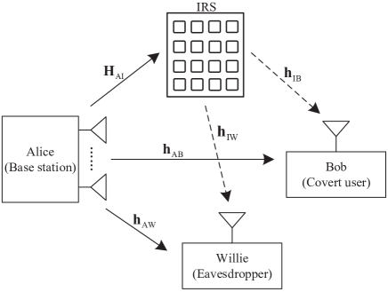
Figure 1: Illustration of the covert communication scenario.

A typical covert communication scenario is illustrated in Fig. 1, in which Alice transmits private data stream ${x_{b}}$ to Bob (covert user). For simplicity, we assume the power of the transmitted signal ${x_{b}}$ is unit, i.e., ${{\mathbb{E}}}\left\{{{{\left|{{x_{\rm{b}}}}\right|}^{2}}}\right\}=1$. At the same time, Willie (eavesdropper) silently (passively) supervise the communication environment and tries to identify whether Bob is receiving signals from Alice or not. To safeguard confidential signals against eavesdropping, an IRS with a smart controller is adopted to assist covert transmission, which is equipped with $M$ reflecting units to coordinate the Alice and IRS for both channel acquisition and data transmission. Specifically, the task for IRS is to adjust the phase shift coefficient of the reflection elements. Then, the signals from Alice is reflected passively to Bob from Alice-Bob link to constructively add with the non-reflected signal, and reflected passively to Willie from Alice-Willie link to destructively add with the non-reflected signal (without generating any extra noise).

In this model, we suppose that Alice is equipped with $N$ antennas, while Bob and Willie each has a single antenna. The channel coefficients from Alice to Bob and Willie, from the IRS to Bob and Willie are defined as ${{\bf{h}}_{\rm{AB}}}\in{\mathbb{C}^{N\times 1}}$, ${{\bf{h}}_{\rm{AW}}}\in{\mathbb{C}^{N\times 1}}$, ${{\bf{h}}_{\rm{IB}}}\in{\mathbb{C}^{M\times 1}}$, and ${{\bf{h}}_{\rm{IW}}}\in{\mathbb{C}^{M\times 1}}$, respectively. Besides, ${{\bf{H}}_{{\rm{AI}}}}\in{\mathbb{C}^{M\times N}}$ is the channel coefficients from Alice to the IRS. Here, ${\mathbb{C}^{N\times M}}$ denotes a ${N\times M}$ complex-valued matrix.

In particular, the large-scale path loss is modeled as ${\rm{PL=}}\sqrt{{\zeta_{0}}{{\left({{d_{0}}/d}\right)}^{\alpha}}}$ for all channels, where ${\zeta_{0}}$ is the path loss at the reference distance ${d_{0}}=1{\rm{m}}$, $\alpha$ is the path loss exponent, and $d$ is the link distance. For the small-scale fading, the channels from Alice to Willie and Bob, the is assumed to be Rayleigh fading, while the IRS-related channels is assumed to be Rician fading, which are represented by

$${{\bf{H}}_{{\rm{AI}}}}=\left({\sqrt{\frac{K_{{\rm{A}}}}{{1+K}}}{\bf{H}}_{{\rm{A}}}^{{\rm{LOS}}}+\sqrt{\frac{1}{{1+{K_{{\rm{A}}}}}}}{\bf{H}}_{{\rm{A}}}^{{\rm{NLOS}}}}\right),$$ (1a)

$${{\bf{h}}_{{\rm{Ij}}}}=\left({\sqrt{\frac{K_{{\rm{j}}}}{{1+K}}}{\bf{h}}_{{\rm{j}}}^{{\rm{LOS}}}+\sqrt{\frac{1}{{1+{K_{{\rm{j}}}}}}}{\bf{h}}_{{\rm{j}}}^{{\rm{NLOS}}}}\right),{\rm{j}}\in\left\{{{\rm{B}},{\rm{W}}}\right\},$$ (1b)

where ${K_{{\rm{j}}}}$ is the Rician factor, and ${\rm{j}}$ denotes ${\rm{B}}$, ${\rm{W}}$ and ${\rm{A}}$. ${\bf{H}}_{{\rm{A}}}^{{\rm{LOS}}}$ and ${\bf{H}}_{{\rm{A}}}^{{\rm{NLOS}}}$ are the deterministic line-of-sight (LoS) and the non-LoS (NLoS) of the Alice-IRS channel, respectively. And the deterministic LoS and the NLoS of the IRS-related channel are represented by ${\bf{h}}_{{\rm{j}}}^{{\rm{LOS}}}$ and ${\bf{h}}_{{\rm{j}}}^{{\rm{NLOS}}}$, respectively. Here, ${\bf{h}}_{{\rm{j}}}^{{\rm{LOS}}}$ is modeled as the product of steering vectors of the transmit and receive arrays, i.e., ${\bf{h}}_{{\rm{j}}}^{{\rm{LOS}}}={{\bf{a}}_{r}}{\bf{a}}_{t}^{H}$, and ${\bf{h}}_{{\rm{j}}}^{{\rm{NLOS}}}$ is modeled as Rayleigh fading. ${{\bf{a}}_{r}}$ and ${{\bf{a}}_{t}}$ are defined as,

$${{\bf{a}}_{r}}={\left[{1,\exp\left({\frac{{j2\pi{d_{t}}}}{\lambda}\sin{\varphi_{t}}}\right),\cdots,\exp\left({\frac{{j2\pi{d_{t}}}}{\lambda}\left({{N_{t}}-1}\right)\sin{\varphi_{t}}}\right)}\right]^{H}},$$ (2a)

$${{\bf{a}}_{t}}={\left[{1,\exp\left({\frac{{j2\pi{d_{r}}}}{\lambda}\sin{\varphi_{r}}}\right),\cdots,\exp\left({\frac{{j2\pi{d_{r}}}}{\lambda}\left({{N_{r}}-1}\right)\sin{\varphi_{r}}}\right)}\right]^{H}}.$$ (2b)

Here, $\lambda$ denotes the frequency of the carrier wave. ${d_{t}}$ and ${d_{r}}$ are the antenna spacing of the transmit and receive array, respectively. We assume that $\lambda=\frac{{{d_{r}}}}{2}=\frac{{{d_{t}}}}{2}$. $\varphi_{t}$ and $\varphi_{r}$ are the angle of departure and the angle of arrival, where ${\varphi_{t}}={\tan^{-1}}\left({\frac{{{y_{r}}-{y_{t}}}}{{{x_{r}}-{x_{t}}}}}\right)$ and ${\varphi_{r}}=\pi-{\varphi_{t}}$, with $\left({{x_{t}},{y_{t}}}\right)$ and $\left({{x_{r}},{y_{r}}}\right)$ being the location of the transmitter and the receiver, respectively. The number of antennas at the transmitter and receiver are denoted as $N_{t}$ and $N_{r}$, respectively.

II-A Signal Model

Let ${{\cal H}_{0}}$ denote the null hypothesis that Alice does not transmit private data stream to Bob, while ${{\cal H}_{1}}$ denotes the alternate hypothesis that Alice transmits private data stream to Bob[17]. From Willie’s perspective, Alice’s transmitted signal is given by

$${\bf{x}}=\left\{\begin{array}[]{l}0,~{}~{}~{}~{}~{}~{}~{}~{}{{\cal H}_{0}}\\ {{\bf{w}}_{\rm{b}}}{x_{\rm{b}}},~{}~{}~{}{{\cal H}_{1}}\\ \end{array}\right.$$ (5)

where ${{\bf{w}}_{\rm{b}}}$ denotes the transmit beamformer vector for ${{x_{{\rm{b}}}}}$. For simplicity, we also assume that Alice does not transmit any signal under ${{\cal H}_{0}}$. The beamformer ${{\bf{w}}_{\rm{b}}}$ satisfies

$${\left\|{{{\bf{w}}_{\rm{b}}}}\right\|^{2}}\leq{P_{{\rm{total}}}},$$ (6)

where ${P_{{\rm{total}}}}$ denotes the maximum transmit power of Alice.

The diagonal matrix ${\bf{Q}}\buildrel\Delta\over{=}{\rm{diag}}\left({\bf{q}}\right)$ is denoted as the phase shift matrix at IRS, which diagonal elements are the corresponding elements of the vector ${\bf{q}}$. Here, ${\bf{q}}\buildrel\Delta\over{=}{\left[{{q_{1}},\cdots,{q_{m}},\cdots,{q_{M}}}\right]^{T}}$ with ${q_{m}}={\beta_{m}}{e^{j{\theta_{m}}}}$, where ${\theta_{m}}\in\left[{0,2\pi}\right)$ and ${\beta_{m}}\in\left[{0,1}\right]$ respectively denote the controllable phase shift and amplitude reflection coefficient, introduced by the $m$th unit for $m=1,\cdots M$. For simplicity, we set ${\beta_{m}}=1,\forall m$, to obtain the maximum gain of the reflecting power. Thus, we have

$$\left|{{q_{m}}}\right|=1,m=1,\cdots M.$$ (7)

Thus, the received signal at Bob is expressed as

$${y_{{\rm{b}}}}=\left\{{\begin{array}[]{*{20}{c}}{z_{\rm{b}}},~{}~{}~{}~{}~{}~{}~{}~{}~{}~{}~{}~{}~{}~{}~{}~{}~{}~{}~{}~{}~{}~{}~{}~{}~{}~{}~{}~{}~{}~{}~{}~{}{{\cal H}_{0}}\\ \left({{\bf{h}}_{{\rm{IB}}}^{H}{\bf{Q}}{{\bf{H}}_{{\rm{AI}}}}+{\bf{h}}_{{\rm{AB}}}^{H}}\right){{\bf{w}}_{\rm{b}}}{x_{\rm{b}}}+{z_{\rm{b}}},~{}{{\cal H}_{1}}\end{array}}\right.$$ (10)

where ${z_{\rm{b}}}\sim{\cal CN}\left({{\rm{0}},\sigma_{\rm{b}}^{2}}\right)$ is the received noise at Bob.

For Willie, the received signal is given by

$${y_{{\rm{w}}}}=\left\{{\begin{array}[]{*{20}{c}}{z_{\rm{w}}},~{}~{}~{}~{}~{}~{}~{}~{}~{}~{}~{}~{}~{}~{}~{}~{}~{}~{}~{}~{}~{}~{}~{}~{}~{}~{}~{}~{}~{}~{}~{}{{\cal H}_{0}}\\ \left({{\bf{h}}_{{\rm{IW}}}^{H}{\bf{Q}}{{\bf{H}}_{{\rm{AI}}}}+{\bf{h}}_{{\rm{AW}}}^{H}}\right){{\bf{w}}_{\rm{b}}}{x_{\rm{b}}}+{z_{\rm{w}}},~{}{{\cal H}_{1}}\end{array}}\right.$$ (13)

where ${z_{\rm{w}}}\sim{\cal CN}\left({{\rm{0}},\sigma_{\rm{w}}^{2}}\right)$ is the received noise at Willie.

According to (10), the instantaneous rate at Bob under hypothesis ${{\cal H}_{1}}$ is given by

$${R_{\rm{b}}}={\log_{2}}\left({1+\frac{{{{\left|{\left({{\bf{h}}_{{\rm{IB}}}^{H}{\bf{Q}}{{\bf{H}}_{{\rm{AI}}}}+{\bf{h}}_{{\rm{AB}}}^{H}}\right){{\bf{w}}_{\rm{b}}}}\right|}^{2}}}}{{\sigma_{\rm{b}}^{2}}}}\right).$$ (14)

II-B Covert Constraints

Since Willie needs to distinguish between the two hypotheses ${{\cal H}_{0}}$ and ${{\cal H}_{1}}$ according to its received signal ${y_{{\rm{w}}}}$, it is necessary to quantify the probability of ${y_{{\rm{w}}}}$. We assume that the likelihood functions of the received signals of Willie under ${{{\cal H}_{\rm{0}}}}$ and ${{{\cal H}_{\rm{1}}}}$ are expressed as ${p_{0}}\left({{y_{\rm{w}}}}\right)$ and ${p_{1}}\left({{y_{\rm{w}}}}\right)$, respectively. Specifically, as per (13), ${p_{0}}\left({{y_{\rm{w}}}}\right)$ and ${p_{1}}\left({{y_{\rm{w}}}}\right)$ are given by

$${p_{0}}\left({{y_{\rm{w}}}}\right)=\frac{1}{{\pi{\lambda_{0}}}}\exp\left({-\frac{{{{\left|{{y_{\rm{w}}}}\right|}^{2}}}}{{{\lambda_{0}}}}}\right),$$ (15a)

$${p_{1}}\left({{y_{\rm{w}}}}\right)=\frac{1}{{\pi{\lambda_{1}}}}\exp\left({-\frac{{{{\left|{{y_{\rm{w}}}}\right|}^{2}}}}{{{\lambda_{1}}}}}\right),$$ (15b)

where ${\lambda_{0}}\buildrel\Delta\over{=}\sigma_{\rm{w}}^{2}$ and ${\lambda_{1}}\buildrel\Delta\over{=}{\left|{\left({{\bf{h}}_{{\rm{IW}}}^{H}{\bf{Q}}{{\bf{H}}_{{\rm{AI}}}}+{\bf{h}}_{{\rm{AW}}}^{H}}\right){{\bf{w}}_{\rm{b}}}}\right|^{\rm{2}}}+\sigma_{\rm{w}}^{2}$.

In general, the prior probabilities of hypotheses ${{{\cal H}_{0}}}$ and ${{{\cal H}_{1}}}$ are assumed to be equal, i.e., each equals to $1/2$. As such, the detection error probability is utilized to evaluate the detection performance, which can be given by [18, 19, 17]

$$\xi=\Pr\left({{{\cal D}_{1}}\left|{{{\cal H}_{0}}}\right.}\right)+\Pr\left({{{\cal D}_{0}}\left|{{{\cal H}_{1}}}\right.}\right),$$ (16)

where ${{\cal D}_{1}}$ indicates that the transmission from Alice to Bob is present, and ${{\cal D}_{0}}$ indicates the other case. In covert communications, Willie aims to minimize the probability of detection error ${\xi}$ based on an optimal detector. To be specific, the covert communication constraint can be written as $\xi\geq 1-\varepsilon$, where $0\leq\varepsilon\leq 1$ is a priori value to specify the covert communication constraint.

In order to incorporate $\xi$ into our problem formulation, we next specify the conditions of the likelihood function so that with the given $\varepsilon$ the covert communication can be achieved (i.e., the constraint can be satisfied). First, let

$$\xi=1-{V_{T}}\left({{p_{0}},{p_{1}}}\right),$$ (17)

where ${V_{T}}\left({{p_{0}},{p_{1}}}\right)$ is the total variation between ${p_{0}}\left({{y_{\rm{w}}}}\right)$ and ${p_{1}}\left({{y_{\rm{w}}}}\right)$. Usually, computing ${V_{T}}\left({{p_{0}},{p_{1}}}\right)$ analytically is intractable. Thus, we adopt Pinsker’s inequality [19], and obtain

$${V_{T}}\left({{p_{0}},{p_{1}}}\right)\leq\sqrt{\frac{1}{2}D\left({{p_{0}}\left\|{{p_{1}}}\right.}\right)},$$ (18a)

$${V_{T}}\left({{p_{0}},{p_{1}}}\right)\leq\sqrt{\frac{1}{2}D\left({{p_{1}}\left\|{{p_{0}}}\right.}\right)},$$ (18b)

where $D\left({{p_{0}}\left\|{{p_{1}}}\right.}\right)$ denotes the Kullback-Leibler (KL) divergence from $p_{0}(y_{\rm{w}})$ to $p_{1}(y_{\rm{w}})$, and $D\left({{p_{1}}\left\|{{p_{0}}}\right.}\right)$ is the KL divergence from $p_{1}(y_{\rm{w}})$ to $p_{0}(y_{\rm{w}})$. $D\left({{p_{0}}\left\|{{p_{1}}}\right.}\right)$ and $D\left({{p_{1}}\left\|{{p_{0}}}\right.}\right)$ are respectively given as

$$D\left({{p_{0}}\left\|{{p_{1}}}\right.}\right) =\int_{-\infty}^{+\infty}{{p_{0}}\left({{y_{\text{w}}}}\right)\ln\frac{{{p_{0}}\left({{y_{\text{w}}}}\right)}}{{{p_{1}}\left({{y_{\text{w}}}}\right)}}}dy=\ln\frac{{{\lambda_{1}}}}{{{\lambda_{0}}}}+\frac{{{\lambda_{0}}}}{{{\lambda_{1}}}}-1,$$ (19a)

$$D\left({{p_{1}}\left\|{{p_{0}}}\right.}\right) =\int_{-\infty}^{+\infty}{{p_{1}}\left({{y_{\text{w}}}}\right)\ln\frac{{{p_{1}}\left({{y_{\text{w}}}}\right)}}{{{p_{0}}\left({{y_{\text{w}}}}\right)}}}dy=\ln\frac{{{\lambda_{0}}}}{{{\lambda_{1}}}}+\frac{{{\lambda_{1}}}}{{{\lambda_{0}}}}-1.$$ (19b)

Therefore, in order to achieve covert communication with the given $\varepsilon$, i.e., $\xi\geq 1-\varepsilon$, the KL divergences of the likelihood functions should satisfy one of the following constraints:

$$D\left({{p_{0}}\left\|{{p_{1}}}\right.}\right)\leq 2{\varepsilon^{2}},$$ (20a)

$$D\left({{p_{1}}\left\|{{p_{0}}}\right.}\right)\leq 2{\varepsilon^{2}}.$$ (20b)

III Proposed Covert Transmission for Perfect WCSI

Practically, we consider a condition that often appears. In this case, Willie is a legitimate user. Alice knows the complete CSI of the channel ${{\bf{h}}_{\rm{IW}}}$ and ${{\bf{h}}_{\rm{AW}}}$, and then uses it to help Bob avoid Willie’s monitoring [20, 21].

Generally, in order to maximize the covert rate to Bob with given vector ${{\bf{w}}_{\rm{b}}}$, the design of the IRS reflecting beamforming vector ${\bf{q}}$ satisfies the following goal. That is, the phase of the reflected channel ${{\bf{h}}_{{\rm{IB}}}^{H}{\bf{Q}}{{\bf{H}}_{{\rm{AI}}}}}$ is aligned with that of the direct channel ${{{\bf{h}}_{{\rm{AB}}}}}$. In this way, we can maximize the received signal power at the user, which is equivalent to maximize ${R_{\rm{b}}}$. Therefore, we maximize the covert rate to Bob by optimizing beamformers ${{\bf{w}}_{\rm{b}}}$ at Alice and the reflecting beamforming vector ${\bf{q}}$ at IRS.

III-A Covert Beamformers Design for Continuous Phase Shifts

Specifically, we study a joint beamforming design problem with the objective of maximizing the achievable covert rate of Bob ${R_{\rm{b}}}$, subject to the perfect covert transmission constraint, the total transmit power constraints of Alice and the IRS-related QoS. This is mathematically expressed as

$$\mathop{\max}\limits_{{{\bf{w}}_{\rm{b}}},{\bf{q}}}{\rm{}} ~{}{R_{\rm{b}}}\hfill$$ (21a)

s.t. $$D\left({{p_{0}}\left\|{{p_{1}}}\right.}\right)=0,\hfill$$ (21b)

$${\left\|{{{\mathbf{w}}_{\rm{b}}}}\right\|^{2}}\leq{P_{{\rm{total}}}},\hfill$$ (21c)

$$\left|{{q_{m}}}\right|=1,\forall m.$$ (21d)

Note that problem (21) is non-convex and difficult to be optimally solved. Moreover, $D\left({{p_{0}}\left\|{{p_{1}}}\right.}\right)=0$ or $D\left({{p_{1}}\left\|{{p_{0}}}\right.}\right)=0$ means that the perfect covert transmission.

Equivalently, problem (21) can be reformulated as

$$\mathop{\max}\limits_{{{\mathbf{w}}_{\rm{b}}},{\bf{q}}}~{} {\left|{\left({{\bf{h}}_{{\rm{IB}}}^{H}{\bf{Q}}{{\bf{H}}_{{\rm{AI}}}}+{\bf{h}}_{{\rm{AB}}}^{H}}\right){{\bf{w}}_{\rm{b}}}}\right|^{2}}$$ (22a)

$${\rm{s.t.}}~{} {\left|{\left({{\bf{h}}_{{\rm{IW}}}^{H}{\bf{Q}}{{\bf{H}}_{{\rm{AI}}}}+{\bf{h}}_{{\rm{AW}}}^{H}}\right){{\bf{w}}_{\rm{b}}}}\right|^{\rm{2}}}=0,$$ (22b)

$${\left\|{{{\mathbf{w}}_{\rm{b}}}}\right\|^{2}}\leq{P_{{\rm{total}}}},\hfill$$ (22c)

$$\left|{{q_{m}}}\right|=1,\forall m.$$ (22d)

Next, we need to solve the following two sub-problems iteratively: fix ${{\mathbf{w}}_{\rm{b}}}$ to optimize ${\bf{q}}$, and then fix ${\bf{q}}$ to optimize ${{\mathbf{w}}_{\rm{b}}}$, which are given in the following two subsections in detail, respectively. Then, the entire algorithm is presented.

III-A1 Sub-Problem 1. Optimizing ${{\mathbf{w}}_{\rm{b}}}$ with Given ${\bf{q}}$

When we fix ${\bf{q}}$, problem (22) can be converted to the following problem

$$\mathop{\max}\limits_{{{\mathbf{w}}_{\rm{b}}}}~{} {\left|{\left({{\bf{h}}_{{\rm{IB}}}^{H}{\bf{Q}}{{\bf{H}}_{{\rm{AI}}}}+{\bf{h}}_{{\rm{AB}}}^{H}}\right){{\bf{w}}_{\rm{b}}}}\right|^{2}}$$ (23)

$${\rm{s.t.}}~{} \eqref{C_14b},\eqref{C_14c}.$$

Let ${{\bf{t}}_{\rm{B}}}\buildrel\Delta\over{=}{\left({{\bf{h}}_{{\rm{IB}}}^{H}{\bf{Q}}{{\bf{H}}_{{\rm{AI}}}}+{\bf{h}}_{{\rm{AB}}}^{H}}\right)}$ and ${{\bf{t}}_{\rm{W}}}\buildrel\Delta\over{=}\left({{\bf{h}}_{{\rm{IW}}}^{H}{\bf{Q}}{{\bf{H}}_{{\rm{AI}}}}+{\bf{h}}_{{\rm{AW}}}^{H}}\right)$. We use the SDR technique, i.e., ${{\bf{W}}_{\rm{b}}}{\rm{=}}{{\bf{w}}_{\rm{b}}}{\bf{w}}_{\rm{b}}^{H}$. By ignoring the rank-one constraints, we obtain a relaxed version of problem (23) as

$$\mathop{\max}\limits_{{{\bf{W}}_{\rm{b}}}}~{} {\rm{Tr}}\left({{\bf{t}}_{\rm{B}}{{\bf{W}}_{\rm{b}}}{{\bf{t}}_{\rm{B}}^{H}}}\right)$$ (24a)

$${\rm{s.t.}}~{} {\rm{Tr}}\left({{\bf{t}}_{\rm{W}}{{\bf{W}}_{\rm{b}}}{{\bf{t}}_{\rm{W}}^{H}}}\right)=0,$$ (24b)

$${\rm{Tr}}\left({{{\bf{W}}_{\rm{b}}}}\right)\leq{P_{{\rm{total}}}},$$ (24c)

$${{{\bf{W}}_{\rm{b}}}}\underline{\succ}{\bf{0}}.$$ (24d)

Denote ${\bf{W}}_{{\rm{b}}}^{*}$ as the optimal solutions of (24). Due to relaxation, the rank of ${\bf{W}}_{{\rm{b}}}^{*}$ may not equal to one. Therefore, if ${\rm{rank}}\left({{\bf{W}}_{{\rm{b}}}^{*}}\right)=1$, the optimal solutions of (23) is ${\bf{W}}_{{\rm{b}}}^{*}$, and the optimal beamformer ${{\bf{w}}_{{\rm{b}}}}$ is solved based on the singular value decomposition (SVD), i.e.,${\bf{W}}_{{\rm{b}}}^{*}={{\bf{w}}_{{\rm{b}}}}{\bf{w}}_{{\rm{b}}}^{H}$. Otherwise, we propose a projection approximation procedure to obtain a high-quality rank-one solution to (24), which is summarized in Algorithm 1.

Proposition 1: Let ${\bf{W}}_{{\rm{b}}}^{*}$ denote the optimal solution of problem (24). If ${\rm{rank}}\left({{\bf{W}}_{{\rm{b}}}^{*}}\right)>1$, then the projection approximation procedure can provide a rank-one solution ${{{\bf{\bar{W}}}}_{\rm{b}}}$ that satisfies constraint (24b) and (24c).

Proof: Please see Appendix A for proof.

Algorithm 1 :Projection approximation procedure for problem (24)

1:Set an SDR solution ${\bf{W}}_{\rm{b}}$, ${\bf{P}}$ denotes the project matrix of vector ${{\bf{W}}_{\rm{b}}^{{1\mathord{\left/{\vphantom{12}}\right.\kern-1.2pt}2}}{\bf{t}}_{\rm{b}}^{H}}$, where ${\bf{P}}=\frac{{{\bf{W}}_{\rm{b}}^{{1\mathord{\left/{\vphantom{12}}\right.\kern-1.2pt}2}}{\bf{t}}_{\rm{b}}^{H}{{\left({{\bf{W}}_{\rm{b}}^{{1\mathord{\left/{\vphantom{12}}\right.\kern-1.2pt}2}}{\bf{t}}_{\rm{b}}^{H}}\right)}^{H}}}}{{{{\left\|{{\bf{t}}_{\rm{b}}^{H}{\bf{W}}_{\rm{b}}^{{1\mathord{\left/{\vphantom{12}}\right.\kern-1.2pt}2}}}\right\|}^{2}}}}$;

2:Construct a new rank one solution ${{{\bf{\bar{W}}}}_{\rm{b}}}={\bf{W}}_{\rm{b}}^{{1\mathord{\left/{\vphantom{12}}\right.\kern-1.2pt}2}}{\bf{PW}}_{\rm{b}}^{{1\mathord{\left/{\vphantom{12}}\right.\kern-1.2pt}2}}$ that satisfies constraint (24b) and (24c);

3:By SVD method, we can obtain ${{{\bf{w}}_{\rm{b}}^{*}}}$ from ${{{\bf{\bar{W}}}}_{\rm{b}}}$ for problem (24).

III-A2 Sub-Problem 2. Optimizing ${\bf{q}}$ with Given ${{\mathbf{w}}_{\rm{b}}}$

When we fix ${{\mathbf{w}}_{\rm{b}}}$, problem (22) can be converted to

$$\mathop{\max}\limits_{{\bf{q}}}~{} {{{{\left|{\left({{\bf{h}}_{{\rm{IB}}}^{H}{\bf{Q}}{{\bf{H}}_{{\rm{AI}}}}+{\bf{h}}_{{\rm{AB}}}^{H}}\right){{\bf{w}}_{\rm{b}}}}\right|}^{2}}}}$$ (25)

$${\rm{s.t.}}~{} \eqref{C_14b},\eqref{C_14d}.$$

Since

$${\bf{h}}_{{\rm{IB}}}^{H}{\bf{Q}}{{\bf{H}}_{{\rm{AI}}}}={{\bf{q}}^{H}}{\rm{diag}}\left({{\bf{h}}_{{\rm{IB}}}^{H}}\right){{\bf{H}}_{{\rm{AI}}}},$$ (26a)

$${\bf{h}}_{{\rm{IW}}}^{H}{\bf{Q}}{{\bf{H}}_{{\rm{AI}}}}={{\bf{q}}^{H}}{\rm{diag}}\left({{\bf{h}}_{{\rm{IW}}}^{H}}\right){{\bf{H}}_{{\rm{AI}}}},$$ (26b)

the following equalities hold:

$${\left|{\left({{\bf{h}}_{{\rm{IB}}}^{H}{\bf{Q}}{{\bf{H}}_{{\rm{AI}}}}+{\bf{h}}_{{\rm{AB}}}^{H}}\right){{\bf{w}}_{\rm{b}}}}\right|^{2}}={{{\bf{\bar{q}}}}^{H}}{{\bf{G}}_{\rm{B}}}{\bf{\bar{q}}}{\rm{+}}{h_{\rm{B}}},$$ (27)

$${\left|{\left({{\bf{h}}_{{\rm{IW}}}^{H}{\bf{Q}}{{\bf{H}}_{{\rm{AI}}}}+{\bf{h}}_{{\rm{AW}}}^{H}}\right){{\bf{w}}_{\rm{b}}}}\right|^{\rm{2}}}={{{\bf{\bar{q}}}}^{H}}{{\bf{G}}_{\rm{W}}}{\bf{\bar{q}}}{\rm{+}}{h_{\rm{W}}},$$ (28)

where ${\bf{\bar{q}}}={\left[{{{\bf{q}}^{H}},1}\right]^{H}}$, ${h_{\rm{B}}}\buildrel\Delta\over{=}{\bf{h}}_{{\rm{AB}}}^{H}{{\bf{w}}_{\rm{b}}}{\bf{w}}_{\rm{b}}^{H}{{\bf{h}}_{{\rm{AB}}}}$ and ${h_{\rm{W}}}\buildrel\Delta\over{=}{\bf{h}}_{{\rm{AW}}}^{H}{{\bf{w}}_{\rm{b}}}{\bf{w}}_{\rm{b}}^{H}{{\bf{h}}_{{\rm{AW}}}}$. In addition, ${{\bf{G}}_{\rm{B}}}$ and ${{\bf{G}}_{\rm{W}}}$ are defined in (31) and (34), shown at the top of next page, respectively.

$${{\bf{G}}_{\rm{B}}}\buildrel\Delta\over{=}\left[{\begin{array}[]{*{20}{c}}{{\rm{diag}}\left({{\bf{h}}_{{\rm{IB}}}^{H}}\right){{\bf{H}}_{{\rm{AI}}}}{{\bf{w}}_{\rm{b}}}{\bf{w}}_{\rm{b}}^{H}{\bf{H}}_{{\rm{AI}}}^{H}{\rm{diag}}\left({{\bf{h}}_{{\rm{IB}}}^{H}}\right)}&{{\rm{diag}}\left({{\bf{h}}_{{\rm{IB}}}^{H}}\right){{\bf{H}}_{{\rm{AI}}}}{{\bf{w}}_{\rm{b}}}{\bf{w}}_{\rm{b}}^{H}{{\bf{h}}_{{\rm{AB}}}}}\\ {{\bf{h}}_{{\rm{AB}}}^{H}{{\bf{w}}_{\rm{b}}}{\bf{w}}_{\rm{b}}^{H}{\bf{H}}_{{\rm{AI}}}^{H}{\rm{diag}}\left({{\bf{h}}_{{\rm{IB}}}^{H}}\right)}&0\end{array}}\right],$$ (31)

$${{\bf{G}}_{\rm{W}}}\buildrel\Delta\over{=}\left[{\begin{array}[]{*{20}{c}}{{\rm{diag}}\left({{\bf{h}}_{{\rm{IW}}}^{H}}\right){{\bf{H}}_{{\rm{AI}}}}{{\bf{w}}_{\rm{b}}}{\bf{w}}_{\rm{b}}^{H}{\bf{H}}_{{\rm{AI}}}^{H}{\rm{diag}}\left({{\bf{h}}_{{\rm{IW}}}^{H}}\right)}&{{\rm{diag}}\left({{\bf{h}}_{{\rm{IW}}}^{H}}\right){{\bf{H}}_{{\rm{AI}}}}{{\bf{w}}_{\rm{b}}}{\bf{w}}_{\rm{b}}^{H}{{\bf{h}}_{{\rm{AW}}}}}\\ {{\bf{h}}_{{\rm{AW}}}^{H}{{\bf{w}}_{\rm{b}}}{\bf{w}}_{\rm{b}}^{H}{\bf{H}}_{{\rm{AI}}}^{H}{\rm{diag}}\left({{\bf{h}}_{{\rm{IW}}}^{H}}\right)}&0\end{array}}\right].$$ (34)

For formula (28), since ${\bf{W}}_{\rm{b}}$ and ${{\bf{G}}_{\rm{W}}}$ are positive semi-definite matrices, we simplify the constraint (22b) to ${{{\bf{\bar{q}}}}^{H}}{{\bf{G}}_{\rm{W}}}{\bf{\bar{q}}}=0$. Then, we can rewrite problem (25) as

$$\mathop{\max}\limits_{{{\bf{\bar{q}}}}}~{} {{{{{\bf{\bar{q}}}}^{H}}{{\bf{G}}_{\rm{B}}}{\bf{\bar{q}}}{\rm{+}}{h_{\rm{B}}}}}$$ (35a)

$${\rm{s.t.}}~{} {{{\bf{\bar{q}}}}^{H}}{{\bf{G}}_{\rm{W}}}{\bf{\bar{q}}}=0,$$ (35b)

$${{{\bf{\bar{q}}}}^{H}}{{\bf{E}}_{{m}}}{\bf{\bar{q}}}=1,\forall m,$$ (35c)

where ${{\bf{E}}_{{m}}}$ is an $M+1$ dimensional matrix, and the ${\left[{{{\bf{E}}_{m}}}\right]_{i,j}}$ is denoted as the $\left({i,j}\right)$th element, satisfies

$${\left[{{{\bf{E}}_{m}}}\right]_{i,j}}=\left\{{\begin{array}[]{*{20}{c}}{1,\begin{array}[]{*{20}{c}}{}\hfil&{}\hfil\end{array}i=j=m,}\\ {0,\begin{array}[]{*{20}{c}}{}\hfil&{}\hfil\end{array}{\rm{otherwise.}}}\end{array}}\right.$$ (40)

It is still hard to find the optimal solution to (35). Next, the SDR is applied to tackle the non-convexity. Let ${\bf{\bar{Q}}}={\bf{\bar{q}}}{{{\bf{\bar{q}}}}^{H}}$, problem (35) is expressed as its relaxed form without considering the constraint of ${\rm{rank}}\left({{\bf{{\bar{Q}}}}}\right)=1$, which is given by

$$\mathop{\max}\limits_{{\bf{\bar{Q}}}}~{} {{\rm{Tr}}\left({{{\bf{G}}_{\rm{B}}}{\bf{\bar{Q}}}}\right){\rm{+}}{h_{\rm{B}}}}$$ (41a)

$${\rm{s}}.{\rm{t}}. {\rm{Tr}}\left({{{\bf{G}}_{\rm{W}}}{\bf{\bar{Q}}}}\right)=0,$$ (41b)

$${\rm{Tr}}\left({{{\bf{E}}_{m}}{\bf{\bar{Q}}}}\right)=1,\forall m,$$ (41c)

$${\bf{\bar{Q}}}\underline{\succ}{\bf{0}}.$$ (41d)

Problem (41) is a convex semidefinite programming (SDP) problem, which can be solved based on the interior-point method. The issue brought by the relaxation of SDR can be similarly handled as we do for problem (41).

III-A3 Covert Beamformer Design Algorithm

In summary, the optimal covert beamformers of problem (22) can be obtained by solving sub-problem $1$ and sub-problem $2$ iteratively, and the overall algorithm is listed in Algorithm 2. The complexity of solving sub-problem $1$ and sub-problem $2$ is ${\cal O}\left({\max{{\left\{{2,N}\right\}}^{4}}\sqrt{N}\log\left({{1\mathord{\left/{\vphantom{1{{\xi_{1}}}}}\right.\kern-1.2pt}{{\xi_{1}}}}}\right)}\right)$ and ${\cal O}\left({{{\left({M+1}\right)}^{4.5}}\log\left({{1\mathord{\left/{\vphantom{1{{\xi_{1}}}}}\right.\kern-1.2pt}{{\xi_{1}}}}}\right)}\right)$ for each iteration, respectively, where ${\xi_{1}}>0$ is the pre-defined accuracy of problem (21) [22, 23]. In Algorithm 2, ${{\bf{1}}_{N}}$ is denoted as an $N\times 1$ vector with all elements being $1$; $R_{\rm{b}}^{\left(k\right)}=f\left({{\bf{w}}_{\rm{b}}^{\left(k\right)},{{\bf{q}}^{\left(k\right)}}}\right)$ is denoted as the objective value of (22), where ${{\bf{w}}_{\rm{b}}^{\left(k\right)}}$ and ${{\bf{q}}^{\left({k}\right)}}$ are the $k$th iteration variables, and $\epsilon>0$ is denoted as a threshold.

Algorithm 2 : Proposed covert beamformer design algorithm

1:Initialization: Set $k=0$, ${\bf{w}}_{\rm{b}}^{\left(0\right)}={{\sqrt{{P_{{\rm{total}}}}}{{\bf{h}}_{{\rm{AB}}}}}\mathord{\left/{\vphantom{{\sqrt{{P_{{\rm{total}}}}}{{\bf{h}}_{{\rm{AB}}}}}{\left\|{{{\bf{h}}_{{\rm{AB}}}}}\right\|}}}\right.\kern-1.2pt}{\left\|{{{\bf{h}}_{{\rm{AB}}}}}\right\|}}$, ${{\bf{q}}^{\left(0\right)}}={{\bf{1}}_{N}}$ and $R_{\rm{b}}^{\left(0\right)}=f\left({{\bf{w}}_{\rm{b}}^{\left(0\right)},{{\bf{q}}^{\left(0\right)}}}\right)$;

2:repeat

3:Set $k=k+1$;

4:With given ${{\bf{q}}^{\left({k-1}\right)}}$, solve problem (24) and apply Algorithm $1$ over ${{\bf{W}}_{\rm{b}}^{\left(k\right)}}$ to obtain an approximate solution ${{\bf{w}}_{\rm{b}}^{\left(k\right)}}$;

5:With given ${{\bf{w}}_{\rm{b}}^{\left(k\right)}}$, solve problem (41) and apply Gaussian randomization over its solution to obtain an approximate solution ${{\bf{q}}^{\left({k}\right)}}$;

6:Set $R_{\rm{b}}^{\left(k\right)}=f\left({{\bf{w}}_{\rm{b}}^{\left(k\right)},{{\bf{q}}^{\left(k\right)}}}\right)$;

7:until $\frac{{R_{\rm{b}}^{\left(k\right)}-R_{\rm{b}}^{\left({k-1}\right)}}}{{R_{\rm{b}}^{\left(k\right)}}}<\epsilon$;

8:Output ${{\bf{w}}_{\rm{b}}^{\left(k\right)}}$ and ${{\bf{q}}^{\left({k}\right)}}$.

III-B Discrete Phase Shifts Design

For discrete phase shifts, we consider that the phase shift at each element of the IRS can only take a finite number of discrete values, which are equally drawn from $\left[{0,2\pi}\right)$. Denote by $L$ the number of bits. Then the set of phase shifts at each element is given by ${\cal{F}}=\left\{{{\rm{0,}}\Delta\theta,\cdots,\Delta\theta\left({K-1}\right)}\right\}$ where $\Delta\theta=\frac{{2\pi}}{K}$ and $K={2^{L}}$.

Similar to question (15), we aim to maximize the achievable covert rate of Bob ${R_{\rm{b}}}$ by jointly optimizing the transmit beamforming ${{\bf{w}}_{\rm{b}}}$ and phase shifts ${{\hat{\theta}}}$, subject to the perfect covert transmission constraint, the total transmit power constraints of Alice and the IRS-related QoS. This is mathematically expressed as

$$\mathop{\max}\limits_{{{\bf{w}}_{\rm{b}}},{{\hat{\theta}}}}{\rm{}} ~{}{R_{\rm{b}}}\hfill$$ (42a)

s.t. $$D\left({{p_{0}}\left\|{{p_{1}}}\right.}\right)=0,\hfill$$ (42b)

$${\left\|{{{\mathbf{w}}_{\rm{b}}}}\right\|^{2}}\leq{P_{{\rm{total}}}},\hfill$$ (42c)

$${\theta_{n}}\in{\cal{F}},\forall n,$$ (42d)

where ${\hat{\theta}}=\left[{{\theta_{1}},\cdots,{\theta_{M}}}\right]$.

Note that problem (42) is non-convex and difficult to be optimally solved.

Similar to the method of solving problem (22), we need to alternately optimize ${{\mathbf{w}}_{\rm{b}}}$ and ${{\hat{\theta}}}$ for the following two sub-problems.

III-B1 Sub-Problem 3. Optimizing ${{\mathbf{w}}_{\rm{b}}}$ with Given ${{\hat{\theta}}}$

When we fix ${{\hat{\theta}}}$, problem (42) can be converted to the following problem

$$\mathop{\max}\limits_{{{\mathbf{w}}_{\rm{b}}}}~{} {\left|{\left({{\bf{h}}_{{\rm{IB}}}^{H}{\bf{Q}}{{\bf{H}}_{{\rm{AI}}}}+{\bf{h}}_{{\rm{AB}}}^{H}}\right){{\bf{w}}_{\rm{b}}}}\right|^{2}}$$ (43)

$${\rm{s.t.}}~{} \eqref{C14bd},\eqref{C14cd}.$$

The handling of this problem is the same as that of sub-problem 1.

III-B2 Sub-Problem 4. Optimizing ${{\hat{\theta}}}$ with Given ${{\mathbf{w}}_{\rm{b}}}$

When we fix ${{\mathbf{w}}_{\rm{b}}}$, problem (42) can be converted to

$$\mathop{\max}\limits_{{{\hat{\theta}}}}~{} {{{{\left|{\left({{\bf{h}}_{{\rm{IB}}}^{H}{\bf{Q}}{{\bf{H}}_{{\rm{AI}}}}+{\bf{h}}_{{\rm{AB}}}^{H}}\right){{\bf{w}}_{\rm{b}}}}\right|}^{2}}}}$$ (44)

$${\rm{s.t.}}~{} \eqref{C14d_d},$$

Since ${{\hat{\theta}}}$ can only take a fixed value, it is difficult to satisfy the equality requirements of constraint (42b), so in the sub-problem $4$ we remove this constraint, and optimize ${{\mathbf{w}}_{\rm{b}}}$ through the sub-problem $3$ to ensure the constraint (42b) is established.

Let $\Phi={\rm{diag}}\left({{\bf{h}}_{{\rm{IB}}}^{H}}\right){{\bf{H}}_{{\rm{AI}}}}{{\bf{w}}_{\rm{b}}}$, ${\bf{A}}=\Phi{\Phi^{H}}$ and ${{{\bf{\bar{h}}}}_{{\rm{AB}}}}=\Phi{{\bf{w}}_{\rm{b}}^{H}}{{\bf{h}}_{{\rm{AB}}}}$. Denote by ${{\bf{A}}_{m,k}}$ and ${{{\bf{\bar{h}}}}_{{\rm{AB}},m}}$ the $\left({m,k}\right)$th and $m$th elements in ${\bf{A}}$ and ${{{\bf{\bar{h}}}}_{{\rm{AB}}}}$, respectively. Then the key to solving (44) by applying alternating optimization lies in the observation that for a given $m\in\left\{{1,\cdots,M}\right\}$, by fixing ${\theta_{k}}$’s, $\forall k\neq m$, the objective function of (44) is linear with respect to ${e^{j{\theta_{m}}}}$, which can be written as

$$2{\mathop{\rm Re}\nolimits}\left\{{{e^{j{\theta_{m}}}}{\varsigma_{m}}}\right\}+\sum\limits_{k\neq m}^{M}{\sum\limits_{i\neq m}^{M}{{{\bf{A}}_{k,i}}{e^{j\left({{\theta_{k}}-{\theta_{i}}}\right)}}}}+C,$$ (45)

where ${\varsigma_{m}}=\sum\nolimits_{k\neq m}^{M}{{{\bf{A}}_{m,k}}{e^{-j{\theta_{k}}}}}+{{{\bf{\bar{h}}}}_{{\rm{AB}},m}}=\left|{{\varsigma_{m}}}\right|{e^{-j{\varphi_{m}}}}$ and $C={{\bf{A}}_{m,m}}+2{\mathop{\rm Re}\nolimits}\left\{{\sum\nolimits_{k\neq m}^{M}{{e^{j{\theta_{k}}}}}{{{\bf{\bar{h}}}}_{{\rm{AB}},k}}}\right\}+{\left\|{{\bf{h}}_{{\rm{AB}}}^{H}{{\bf{w}}_{\rm{b}}}}\right\|^{2}}$. Based on (45), it is not difficult to verify that the optimal $m$th phase shift is given by [24]

$$\theta_{m}^{*}=\arg\mathop{\min}\limits_{\theta\in{\cal{F}}}\left|{\theta-{\varphi_{m}}}\right|.$$ (46)

III-B3 Discrete Phase Shifts Algorithm

In summary, the optimal covert beamformers of problem (42) can be obtained by solving sub-problem $3$ and sub-problem $4$ iteratively, and the overall algorithm is similar to Algorithm $2$.

Note that the algorithm requires a proper choice of initial discrete phase shifts ${{{\hat{\theta}}}^{\left(0\right)}}$, which can be obtained by solving the problem (15), and then quantizing the continuous phase shifts obtained to the nearest points in ${\cal{F}}$ similarly as (46).

IV Proposed Robust Covert Transmission for Imperfect WCSI

In many other cases, the WCSI may not be always accessible to Alice because of the potential limited cooperation between Alice and Willie. We consider another practical scenario where Willie is a regular user with only limited cooperation to Alice. In this case, Alice has imperfect CSI knowledge due to the passive warden [25] and channel estimation errors [26, 21]. Here, the imperfect WCSI is modeled as

$${{\bf{h}}_{\rm{AW}}}={{{\bf{\hat{h}}}}_{\rm{AW}}}+\Delta{{\bf{h}}_{\rm{AW}}},$$ (47)

and

$${{\bf{h}}_{\rm{IW}}}={{{\bf{\hat{h}}}}_{\rm{IW}}}+\Delta{{\bf{h}}_{\rm{IW}}},$$ (48)

where ${{{\bf{\hat{h}}}}_{\rm{AW}}}$ and ${{{\bf{\hat{h}}}}_{\rm{IW}}}$ denote the estimated CSI vector between Alice and Willie, between Willie and IRS, respectively. $\Delta{{\bf{h}}_{\rm{AW}}}$ and $\Delta{{\bf{h}}_{\rm{IW}}}$ denote the corresponding CSI error vectors. Moreover, $\Delta{{\bf{h}}_{\rm{AW}}}$ and $\Delta{{\bf{h}}_{\rm{IW}}}$ are characterized by an ellipsoidal region, i.e.,

$${{\cal E}_{\rm{AW}}}\buildrel\Delta\over{=}\left\{{\Delta{{\bf{h}}_{\rm{AW}}}\left|{\Delta{\bf{h}}_{\rm{AW}}^{H}{{\bf{C}}_{\rm{AW}}}\Delta{{\bf{h}}_{\rm{AW}}}\leq{v_{\rm{AW}}}}\right.}\right\},$$ (49)

and

$${{\cal E}_{\rm{IW}}}\buildrel\Delta\over{=}\left\{{\Delta{{\bf{h}}_{\rm{IW}}}\left|{\Delta{\bf{h}}_{\rm{IW}}^{H}{{\bf{C}}_{\rm{IW}}}\Delta{{\bf{h}}_{\rm{IW}}}\leq{v_{\rm{IW}}}}\right.}\right\},$$ (50)

where ${{\bf{C}}_{\rm{AW}}}={{\bf{C}}_{\rm{AW}}^{H}}\underline{\succ}{\bf{0}}$, ${{\bf{C}}_{\rm{IW}}}={{\bf{C}}_{\rm{IW}}^{H}}\underline{\succ}{\bf{0}}$ control the axes of the ellipsoid, and ${v_{\rm{AW}}}>0$, ${v_{\rm{IW}}}>0$ determine the volume of the ellipsoid [8, 29].

IV-A Willie’s Detection Performance

Based on the model described above, we investigate the optimal decision threshold of Willie, and derive the corresponding false alarm and miss detection probabilities. We focus on the worst case scenario for covert transmission, in which the beamformers ${\mathbf{w}}_{\rm{b}}$ is known by Willie.

According to the Neyman-Pearson criterion [17], the likelihood ratio test is considered as the the optimal rule of the detection error minimization [17] , which is expressed as

$$\frac{{{p_{1}}\left({{y_{\rm{w}}}}\right)}}{{{p_{0}}\left({{y_{\rm{w}}}}\right)}}\frac{{\mathop{>}\limits^{{{\cal D}_{1}}}}}{{\mathop{<}\limits_{{{\cal D}_{0}}}}}1,$$ (51)

where ${{{\cal D}_{1}}}$ and ${{{\cal D}_{0}}}$ are the binary decisions corresponding to hypotheses ${{{\cal H}_{1}}}$ and ${{{\cal H}_{0}}}$, respectively, as we defined previously. Furthermore, equation (51) can be reformulated as

$${\left|{{y_{\rm{w}}}}\right|^{2}}\frac{{\mathop{>}\limits^{{{\cal D}_{1}}}}}{{\mathop{<}\limits_{{{\cal D}_{0}}}}}{\phi^{*}}.$$ (52)

In (52), ${\phi^{*}}$ is the optimal threshold for ${\left|{{y_{\rm{w}}}}\right|^{2}}$, which is given by

$${\phi^{*}}\buildrel\Delta\over{=}\frac{{{\lambda_{0}}{\lambda_{1}}}}{{{\lambda_{1}}-{\lambda_{0}}}}{\rm{ln}}\frac{{{\lambda_{1}}}}{{{\lambda_{0}}}}.$$ (53)

Note that, $\lambda_{0}$ and $\lambda_{1}$ are given in (15), and they depend on the beamformer vectors ${\mathbf{w}}_{\rm{b}}$ and the IRS reflect beamforming vector ${\bf{q}}$.

Following (15), the cumulative density functions (CDFs) of ${\left|{{y_{\rm{w}}}}\right|^{2}}$ under ${{{\cal H}_{\rm{0}}}}$ and ${{{\cal H}_{\rm{1}}}}$ are respectively given by

$$\Pr\left({{{\left|{{y_{\rm{w}}}}\right|}^{2}}|{\cal{H}_{\rm{0}}}}\right)=1-\exp\left({-\frac{{{{\left|{{y_{\rm{w}}}}\right|}^{2}}}}{{{\lambda_{0}}}}}\right),$$ (54a)

$$\Pr\left({{{\left|{{y_{\rm{w}}}}\right|}^{2}}|{\cal{H}_{\rm{1}}}}\right)=1-\exp\left({-\frac{{{{\left|{{y_{\rm{w}}}}\right|}^{2}}}}{{{\lambda_{1}}}}}\right).$$ (54b)

Therefore, based on the optimal detection threshold ${\phi^{*}}$, the false alarm $P\left({{{\cal D}_{1}}\left|{{{\cal H}_{0}}}\right.}\right)$ and missed detection probabilities $P\left({{{\cal D}_{0}}\left|{{{\cal H}_{1}}}\right.}\right)$ are given as

$$P\left({{{\cal D}_{1}}\left|{{{\cal H}_{0}}}\right.}\right)={\Pr}\left({{{\left|{{y_{\rm{w}}}}\right|}^{2}}\geq{\phi^{*}}|{{{\cal H}_{\rm{0}}}}}\right)={\left({\frac{{{\lambda_{1}}}}{{{\lambda_{0}}}}}\right)^{-\frac{{{\lambda_{1}}}}{{{\lambda_{1}}-{\lambda_{0}}}}}},$$ (55a)

$$P\left({{{\cal D}_{0}}\left|{{{\cal H}_{1}}}\right.}\right)={\Pr}\left({{{\left|{{y_{\rm{w}}}}\right|}^{2}}\leq{\phi^{*}}|{{{\cal H}_{\rm{1}}}}}\right)=1-{\left({\frac{{{\lambda_{1}}}}{{{\lambda_{0}}}}}\right)^{-\frac{{{\lambda_{0}}}}{{{\lambda_{1}}-{\lambda_{0}}}}}}.$$ (55b)

Let use $P\left({{{\cal D}_{1}}\left|{{{\cal H}_{0}}}\right.}\right)$ and $P\left({{{\cal D}_{0}}\left|{{{\cal H}_{1}}}\right.}\right)$ to characterize the ideal detection performance of Willie. Such results can be used as the theoretical benchmark to measure the covert performance of the robust beamforming design. We will further discuss the detection performance of Willie in the next section.

In practice, it is common that the obtained CSI is corrupted by certain estimation errors [30, 31], which makes the perfect covert transmission, i.e., $D\left({{p_{0}}\left\|{{p_{1}}}\right.}\right)=0$, difficult to be achieved. Thus, we apply adopting $D\left({{p_{0}}\left\|{{p_{1}}}\right.}\right)\leq 2{\varepsilon^{2}}$ and $D\left({{p_{1}}\left\|{{p_{0}}}\right.}\right)\leq 2{\varepsilon^{2}}$ given by (20) as covertness constraints[20, 30, 31, 18].

IV-B Case of $D\left({{p_{0}}\left\|{{p_{1}}}\right.}\right)\leq 2{\varepsilon^{2}}$

To be specific, we aim to maximize ${R_{\rm{b}}}$ via the joint design of the beamformers ${{\bf{w}}_{\rm{b}}}$ and the IRS reflect beamforming vector ${\bf{q}}$, under the IRS-related QoS, the covertness constraint and the total power constraint. Mathematically, the robust covert rate maximization problem is formulated as

$$\mathop{\max}\limits_{{{\bf{w}}_{\rm{b}}},{\bf{q}}}{\rm{}} ~{}{R_{\rm{b}}}\hfill$$ (56a)

s.t. $$D\left({{p_{0}}\left\|{{p_{1}}}\right.}\right)\leq 2{\varepsilon^{2}},\hfill$$ (56b)

$${\left\|{{{\mathbf{w}}_{\rm{b}}}}\right\|^{2}}\leq{P_{{\rm{total}}}},\hfill$$ (56c)

$$\left|{{q_{m}}}\right|=1,\forall m,$$ (56d)

$${{\bf{h}}_{\rm{IW}}}={{{\bf{\hat{h}}}}_{\rm{IW}}}+\Delta{{\bf{h}}_{\rm{IW}}},$$ (56e)

$${{\bf{h}}_{\rm{AW}}}={{{\bf{\hat{h}}}}_{\rm{AW}}}+\Delta{{\bf{h}}_{\rm{AW}}}.$$ (56f)

It can be seen that problem (56) is nonconvex, which is difficult to solve it directly. To tackle this issue, we reformulate the covertness constraint (56b) by exploiting the property of the function $f\left(x\right)=\ln x+\frac{1}{x}-1$ for $x>0$. Specifically, the covertness constraint $D\left({{p_{0}}\left\|{{p_{1}}}\right.}\right)=\ln\frac{{{\lambda_{1}}}}{{{\lambda_{0}}}}+\frac{{{\lambda_{0}}}}{{{\lambda_{1}}}}-1\leq 2{\varepsilon^{2}}$ can be equivalently transformed as

$$\bar{a}\leq\frac{{{\lambda_{1}}}}{{{\lambda_{0}}}}\leq\bar{b},$$ (57)

where $\bar{a}$ and $\bar{b}$ are the two roots of the equation $\ln\frac{{{\lambda_{1}}}}{{{\lambda_{0}}}}+\frac{{{\lambda_{0}}}}{{{\lambda_{1}}}}-1=2{\varepsilon^{2}}$. Therefore, constraint (56b) can be equivalently reformulated as

$$\bar{a}\leq\frac{{{\left|{\left({{\bf{h}}_{{\rm{IW}}}^{H}{\bf{Q}}{{\bf{H}}_{{\rm{AI}}}}+{\bf{h}}_{{\rm{AW}}}^{H}}\right){{\bf{w}}_{\rm{b}}}}\right|^{\rm{2}}}+\sigma_{\rm{w}}^{2}}}{{\sigma_{\rm{w}}^{2}}}\leq\bar{b}.$$ (58)

Here, due to $\Delta{{\bf{h}}_{\rm{AW}}}\in{{\cal{E}}_{\rm{AW}}}$ and $\Delta{{\bf{h}}_{\rm{IW}}}\in{{\cal{E}}_{\rm{IW}}}$, there are infinite choices for $\Delta{{\bf{h}}_{\rm{AW}}}$ or $\Delta{{\bf{h}}_{\rm{IW}}}$, in constraint (56e) and (56f), respectively. This makes the problem (56) non-convex and difficult to be solved. To overcome this challenge, a relaxation and restriction method are proposed. Specifically, in the relaxation step, the nonconvex problem is converted into a convex SDP; in the restriction step, a finite number of linear matrix inequalities (LMIs) are used to reformulate infinite number of complex constraints.

Similar to the idea of solving problem (22), firstly, we can alternately optimize ${{\mathbf{w}}_{\rm{b}}}$ and ${\bf{q}}$ for problem (56).

IV-B1 Sub-Problem 5. Optimizing ${{\mathbf{w}}_{\rm{b}}}$ with given ${\bf{q}}$

We first optimize the beamformer ${{\mathbf{w}}_{\rm{b}}}$ by fixing ${\bf{q}}$ under constraints (56b), (56c), (56e) and (56f). For mathematical convenience, we define ${{\bf{g}}_{\rm{B}}}{\rm{=}}{\left[{\begin{array}[]{*{20}{c}}{{\bf{h}}_{{\rm{IB}}}^{H}{\bf{Q}}{{\bf{H}}_{{\rm{AI}}}}}&{{\bf{h}}_{{\rm{AB}}}^{H}}\end{array}}\right]^{H}}$, ${{\bf{g}}_{\rm{W}}}{\rm{=}}{\left[{\begin{array}[]{*{20}{c}}{{\bf{h}}_{{\rm{IW}}}^{H}{\bf{Q}}{{\bf{H}}_{{\rm{AI}}}}}&{{\bf{h}}_{{\rm{AW}}}^{H}}\end{array}}\right]^{H}}$ and ${{{\bf{\hat{w}}}}_{\rm{b}}}{\rm{=}}\left[{\begin{array}[]{*{20}{c}}{{{\bf{w}}_{\rm{b}}}}\\ {{{\bf{w}}_{\rm{b}}}}\end{array}}\right]$. Then, the problem can be given as

$$\mathop{\max}\limits_{{{{\bf{\hat{w}}}}_{\rm{b}}}}{\rm{}}~{} {{{{\left|{{\bf{g}}_{\rm{B}}^{H}{{{\bf{\hat{w}}}}_{\rm{b}}}}\right|}^{2}}}}$$ (59a)

s.t. $$\sigma_{\rm{w}}^{2}\left({\bar{a}{\rm{-1}}}\right)\leq{\left|{{\bf{g}}_{\rm{W}}^{H}{{{\bf{\hat{w}}}}_{\rm{b}}}}\right|^{\rm{2}}}\leq\sigma_{\rm{w}}^{2}\left({\bar{b}{\rm{-1}}}\right),\hfill$$ (59b)

$${\left\|{{{\bf{e}}_{1}}{{{\bf{\hat{w}}}}_{\rm{b}}}}\right\|^{2}}\leq{P_{{\rm{total}}}},$$ (59c)

$${{\bf{g}}_{\rm{W}}}={{{\bf{\hat{g}}}}_{\rm{W}}}+\Delta{{\bf{g}}_{\rm{W}}},\Delta{{\bf{g}}_{\rm{W}}}\in{{\cal E}_{\rm{W}}},$$ (59d)

where ${{\bf{e}}_{1}}=\left[{\underbrace{1,\cdots,{\rm{1}}}_{N}{\rm{,}}\underbrace{{\rm{0,}}\cdots{\rm{,0}}}_{N}}\right]$, ${{\cal E}_{\rm{W}}}\buildrel\Delta\over{=}\left\{{\Delta{{\bf{g}}_{\rm{W}}}\left|{\Delta{\bf{g}}_{\rm{W}}^{H}{{\bf{C}}_{\rm{W}}}\Delta{{\bf{g}}_{\rm{W}}}\leq{v_{\rm{W}}}}\right.}\right\}$, and ${v_{\rm{W}}}={v_{{\rm{AW}}}}+{v_{{\rm{IW}}}}$.

To handle the non-convexity issue, we relax the constraint (59b) to a convex form by applying SDR as well. By relaxing ${\widehat{\bf{W}}_{\rm{b}}}={{{\bf{\hat{w}}}}_{\rm{b}}}{\bf{\hat{w}}}_{\rm{b}}^{H}$ to ${\widehat{\bf{W}}_{\rm{b}}}\succeq{\bf{0}}$, the constraint can be equivalently re-expressed as

$$\Delta{\bf{g}}_{\rm{W}}^{H}{\widehat{\bf{W}}_{\rm{b}}}\Delta{{\bf{g}}_{\rm{W}}}+2\Delta{\bf{g}}_{\rm{W}}^{H}{\widehat{\bf{W}}_{\rm{b}}}{{{\bf{\hat{g}}}}_{\rm{W}}}+{\bf{\hat{g}}}_{\rm{W}}^{H}{\widehat{\bf{W}}_{\rm{b}}}{{{\bf{\hat{g}}}}_{\rm{W}}}\geq\sigma_{\rm{w}}^{2}\left({\bar{a}-1}\right),$$ (60a)

$$\Delta{\bf{g}}_{\rm{W}}^{H}{\widehat{\bf{W}}_{\rm{b}}}\Delta{{\bf{g}}_{\rm{W}}}+2\Delta{\bf{g}}_{\rm{W}}^{H}{\widehat{\bf{W}}_{\rm{b}}}{{{\bf{\hat{g}}}}_{\rm{W}}}+{\bf{\hat{g}}}_{\rm{W}}^{H}{\widehat{\bf{W}}_{\rm{b}}}{{{\bf{\hat{g}}}}_{\rm{W}}}\leq\sigma_{\rm{w}}^{2}\left({\bar{b}-1}\right),$$ (60b)

where ${{{\bf{\hat{g}}}}_{\rm{W}}}\buildrel\Delta\over{=}{\left[{\begin{array}[]{*{20}{c}}{{\bf{\hat{h}}}_{{\rm{IW}}}^{H}{\bf{Q}}{{\bf{H}}_{{\rm{AI}}}}}&{{\bf{\hat{h}}}_{{\rm{AW}}}^{H}}\end{array}}\right]^{H}}$ and $\Delta{{\bf{g}}_{\rm{W}}}\buildrel\Delta\over{=}{\left[{\begin{array}[]{*{20}{c}}{\Delta{\bf{h}}_{{\rm{IW}}}^{H}{\bf{Q}}{{\bf{H}}_{{\rm{AI}}}}}&{\Delta{\bf{h}}_{{\rm{AW}}}^{H}}\end{array}}\right]^{H}}$.

By applying SDR, we ignore the rank-one constraints of ${\widehat{\bf{W}}_{\rm{b}}}$, which is similar to the approach used in (23) and (24). Then, problem (59) can be relaxed as follows

$$\mathop{\max}\limits_{{\widehat{\bf{W}}_{\rm{b}}}}{\rm{}}~{} {\rm{Tr}}\left({{\bf{g}}_{\rm{B}}^{H}{{\widehat{\bf{W}}}_{\rm{b}}}{\bf{g}}_{\rm{B}}}\right)$$ (61a)

s.t. $${\rm{Tr}}\left({{{\bf{e}}_{1}}{{\widehat{\bf{W}}}_{\rm{b}}}{\bf{e}}_{1}^{H}}\right)\leq{P_{{\rm{total}}}},$$ (61b)

$${\widehat{\bf{W}}_{\rm{b}}}\underline{\succ}{\bf{0}},$$ (61c)

$$\Delta{{\bf{g}}_{\rm{W}}}\in{{\cal E}_{\rm{W}}},$$ (61d)

$$\eqref{W1a},\eqref{W1b}.$$

It is worth pointing out that the SDR problem (61) is quasi-convex as the objective function and constraints are linear in ${\widehat{\bf{W}}_{\rm{b}}}$. However, problem (61) is still computationally intractable because it involves an infinite number of constraints due to $\Delta{{\bf{g}}_{\rm{W}}}\in{{\cal E}_{\rm{W}}}$.

In the following, we employ S-Lemma to recast the infinitely many constraints as a certain set of LMIs, which is a tractable approximation.

Lemma 1 (S-Lemma[32]): Let ${{\bf{A}}_{m}}\in{{\mathbb{H}}^{N}}$, ${{\bf{b}}_{m}}\in{{\mathbb{C}}^{N\times 1}}$, and ${c_{m}}\in{{\mathbb{R}}^{1\times 1}}$. Denote a function ${f_{m}}\left(x\right),m\in\left\{{1,2}\right\},x\in{{\mathbb{C}}^{N\times 1}}$, we have

$${f_{m}}\left(x\right)={{\bf{x}}^{H}}{{\bf{A}}_{m}}{\bf{x}}+2{\rm Re}\left\{{{\bf{b}}_{m}^{\rm{H}}{\bf{x}}}\right\}+{c_{m}}.$$ (62)

Then, ${f_{1}}\left(x\right)\leq 0\Rightarrow{f_{2}}\left(x\right)\leq 0$ holds if and only if there exits a variable ${\eta}\geq 0$ such that

$${\eta}\left[{\begin{array}[]{*{20}{c}}{{{\bf{A}}_{1}}}&{{{\bf{b}}_{1}}}\\ {{\bf{b}}_{1}^{{H}}}&{{c_{1}}}\end{array}}\right]-\left[{\begin{array}[]{*{20}{c}}{{{\bf{A}}_{2}}}&{{{\bf{b}}_{2}}}\\ {{\bf{b}}_{2}^{{H}}}&{{c_{2}}}\end{array}}\right]\underline{\succ}{\bf{0}}.$$ (67)

Consequently, by using S-Lemma, constraints (60a) and (60b) can be respectively given as a finite number of LMIs:

$$\left[{\begin{array}[]{*{20}{c}}{{{\widehat{\bf{W}}}_{\rm{b}}}+{\eta_{1}}{{\bf{C}}_{\rm{w}}}}&{{{\widehat{\bf{W}}}_{\rm{b}}}{{{\bf{\hat{g}}}}_{\rm{W}}}}\\ {{\bf{\hat{g}}}_{\rm{W}}^{H}{{\widehat{\bf{W}}}_{\rm{b}}}}&{{\bf{\hat{g}}}_{\rm{W}}^{H}{{\widehat{\bf{W}}}_{\rm{b}}}{{{\bf{\hat{g}}}}_{\rm{W}}}-\sigma_{\rm{w}}^{2}\left({\bar{a}-1}\right)-{\eta_{1}}{v_{\rm{W}}}}\end{array}}\right]\underline{\succ}{\bf{0}},$$ (68c)

$$\left[{\begin{array}[]{*{20}{c}}{-{{\widehat{\bf{W}}}_{\rm{b}}}+{\eta_{2}}{{\bf{C}}_{\rm{w}}}}&{-{{\widehat{\bf{W}}}_{\rm{b}}}{{{\bf{\hat{g}}}}_{\rm{W}}}}\\ {-{\bf{\hat{g}}}_{\rm{W}}^{H}{{\widehat{\bf{W}}}_{\rm{b}}}}&{-{\bf{\hat{g}}}_{\rm{W}}^{H}{{\widehat{\bf{W}}}_{\rm{b}}}{{{\bf{\hat{g}}}}_{\rm{W}}}+\sigma_{\rm{w}}^{2}\left({\bar{b}-1}\right)-{\eta_{2}}{v_{\rm{W}}}}\end{array}}\right]\underline{\succ}{\bf{0}}.$$ (68f)

Therefore, we obtain the conservative approximation of (61) as follows:

$$\mathop{\max}\limits_{{\widehat{\bf{W}}_{\rm{b}}}}{\rm{}}~{} {\rm{Tr}}\left({{{\bf{g}}_{\rm{B}}^{H}}{{\widehat{\bf{W}}}_{\rm{b}}}{\bf{g}}_{\rm{B}}}\right)$$ (69)

$${\rm{s}}.{\rm{t}}.~{} \eqref{2sub1sdra},\eqref{2sub1sdrc},\eqref{slemma1},\eqref{slemma2}.$$

Problem (69) is a convex SDP problem which can be optimally solved with the interior-point method. Similarly, let ${\widehat{\bf{W}}_{\rm{b}}}^{opt}$ denotes the optimal solutions of problem (69). If ${\rm{rank}}\left({{\widehat{\bf{W}}_{\rm{b}}}^{opt}}\right)=1$, ${\widehat{\bf{W}}_{\rm{b}}}^{opt}$ is the optimal solutions of problem (69), and the optimal beamformer ${{{\bf{\hat{w}}}}_{\rm{b}}}$ can be obtained by SVD, i.e.,${\widehat{\bf{W}}_{\rm{b}}}^{opt}={{{\bf{\hat{w}}}}_{\rm{b}}}{{{\bf{\hat{w}}}}_{\rm{b}}}^{H}$. Otherwise, if ${\rm{rank}}\left({{\widehat{\bf{W}}_{\rm{b}}}^{opt}}\right)>1$, the Gaussian randomization procedure [22] is adopted to produce a high-quality rank-one solution to (69).

IV-B2 Sub-Problem 6. Optimizing ${\bf{q}}$ with given ${{\mathbf{w}}_{\rm{b}}}$

Now we consider the design of ${\bf{q}}$ on the basis of fixing ${{\mathbf{w}}_{\rm{b}}}$. In this case, the problem (56) can be converted into the following form:

$$\mathop{\max}\limits_{{\bf{q}}}~{} {{{{\left|{\left({{\bf{h}}_{{\rm{IB}}}^{H}{\bf{Q}}{{\bf{H}}_{{\rm{AI}}}}+{\bf{h}}_{{\rm{AB}}}^{H}}\right){{\bf{w}}_{\rm{b}}}}\right|}^{2}}}}$$ (70a)

$${\rm{s.t.}}~{} \bar{a}\leq\frac{{{\left|{\left({{\bf{h}}_{{\rm{IW}}}^{H}{\bf{Q}}{{\bf{H}}_{{\rm{AI}}}}+{\bf{h}}_{{\rm{AW}}}^{H}}\right){{\bf{w}}_{\rm{b}}}}\right|^{\rm{2}}}+\sigma_{\rm{w}}^{2}}}{{\sigma_{\rm{w}}^{2}}}\leq\bar{b},$$ (70b)

$$\left|{{q_{m}}}\right|=1,\forall m.$$ (70c)

Since (56e) and (56f) have been discussed in sub-problem 5, we do not consider these two constraints in sub-problem 6. As a result, the processing method is the same as that of question (25). The SDR is applied to tackle the non-convexity with ${\bf{\bar{Q}}}={\bf{\bar{q}}}{{{\bf{\bar{q}}}}^{H}}$ and ${\bf{\bar{q}}}={\left[{{{\bf{q}}^{H}},1}\right]^{H}}$. Then, (70) is expressed as its relaxed form without considering the ${\rm{rank}}\left({{\bf{{\bar{Q}}}}}\right)=1$ constraint, which is given by

$$\mathop{\max}\limits_{{\bf{\bar{Q}}}}~{} {{\rm{Tr}}\left({{{\bf{G}}_{\rm{B}}}{\bf{\bar{Q}}}}\right){\rm{+}}{h_{\rm{B}}}}$$ (71a)

$${\rm{s}}.{\rm{t}}. \sigma_{\rm{w}}^{2}\left({\bar{a}-1}\right)\leq{\rm{Tr}}\left({{{\bf{G}}_{\rm{W}}}{\bf{\bar{Q}}}}\right){\rm{+}}{h_{\rm{W}}}\leq\sigma_{\rm{w}}^{2}\left({\bar{b}-1}\right),$$ (71b)

$${\rm{Tr}}\left({{{\bf{E}}_{m}}{\bf{\bar{Q}}}}\right)=1,\forall m,$$ (71c)

$${\bf{\bar{Q}}}\underline{\succ}{\bf{0}}.$$ (71d)

Problem (71) is a convex SDP problem, which can be optimally solved with the interior-point method. Also, we may apply the similar technique as we do for problem (69) to deal with the issue brought by the relaxation of SDR.

IV-B3 Robust covert beamformers design algorithm

In short, the robust covert beamformers in problem (56) can be design by solving sub-problem 5 and sub-problem 6 alternately, and the overall algorithm is presented in Algorithm 3. Similar to problem (21) , the complexity of sub-problem $5$ is ${\cal O}\left({\max{{\left\{{3,N}\right\}}^{4}}\sqrt{N}\log\left({{1\mathord{\left/{\vphantom{1{{\xi_{1}}}}}\right.\kern-1.2pt}{{\xi_{2}}}}}\right)}\right)$ for each iteration, and the complexity of sub-problem $6$ is ${\cal O}\left({{{\left({M+1}\right)}^{4.5}}\log\left({{1\mathord{\left/{\vphantom{1{{\xi_{1}}}}}\right.\kern-1.2pt}{{\xi_{2}}}}}\right)}\right)$ for each iteration. ${\xi_{2}}>0$ is the pre-defined accuracy of problem (56) [22, 23]. Here, $R_{\rm{b}}^{\left(k\right)}=f\left({{\bf{w}}_{\rm{b}}^{\left(k\right)},{{\bf{q}}^{\left(k\right)}}}\right)$ is denoted as the objective value of (56), where ${{\bf{w}}_{\rm{b}}^{\left(k\right)}}$ and ${{\bf{q}}^{\left({k}\right)}}$ are the $k$th iteration variables.

Algorithm 3 : Proposed robust covert beamformers design algorithm

1:Initialization: Set $k=0$, ${\bf{w}}_{\rm{b}}^{\left(0\right)}=\frac{{\sqrt{{P_{{\rm{total}}}}}{{\bf{h}}_{{\rm{AB}}}}}}{{\left\|{{{\bf{h}}_{{\rm{AB}}}}}\right\|}}$, ${{\bf{q}}^{\left(0\right)}}={{\bf{1}}_{N}}$, and $R_{\rm{b}}^{\left(0\right)}=f\left({{\bf{w}}_{\rm{b}}^{\left(0\right)},{{\bf{q}}^{\left(0\right)}}}\right)$;

2:repeat

3:Set $k=k+1$;

4:With given ${{\bf{q}}^{\left({k-1}\right)}}$, solve problem (69) and apply Gaussian randomization over its solution to obtain an approximate solution ${{\bf{w}}_{\rm{b}}^{\left(k\right)}}$;

5:With given ${{\bf{w}}_{\rm{b}}^{\left(k\right)}}$, solve problem (71) and apply Gaussian randomization over ${\bf{\bar{Q}}}^{\left(k\right)}$ to obtain an approximate solution ${{\bf{q}}^{\left({k}\right)}}$;

6:Set $R_{\rm{b}}^{\left(k\right)}=f\left({{\bf{w}}_{\rm{b}}^{\left(k\right)},{{\bf{q}}^{\left(k\right)}}}\right)$;

7:until $\frac{{R_{\rm{b}}^{\left(k\right)}-R_{\rm{b}}^{\left({k-1}\right)}}}{{R_{\rm{b}}^{\left(k\right)}}}<\epsilon$;

8:Output ${{\bf{w}}_{\rm{b}}^{\left(k\right)}}$ and ${{\bf{q}}^{\left({k}\right)}}$.

IV-C Case of $D\left({{p_{1}}\left\|{{p_{0}}}\right.}\right)\leq 2{\varepsilon^{2}}$

In this subsection, the case with constraint $D\left({{p_{1}}\left\|{{p_{0}}}\right.}\right)\leq 2{\varepsilon^{2}}$ is considered. The corresponding robust covert rate maximization problem is given by

$$\mathop{\max}\limits_{{{\bf{w}}_{\rm{b}}},{\bf{q}}}{\rm{}} {R_{\rm{b}}}\left({{{\bf{w}}_{{\rm{c}},1}}},{{{\bf{w}}_{{\rm{b}}}}}\right)\hfill$$ (72a)

s.t. $$D\left({{p_{1}}\left\|{{p_{0}}}\right.}\right)\leq 2{\varepsilon^{2}},\hfill$$ (72b)

$${\left\|{{{\mathbf{w}}_{\rm{b}}}}\right\|^{2}}\leq{P_{{\rm{total}}}},\hfill$$ (72c)

$$\left|{{q_{m}}}\right|=1,\forall m,$$ (72d)

$${{\bf{h}}_{\rm{IW}}}={{{\bf{\hat{h}}}}_{\rm{IW}}}+\Delta{{\bf{h}}_{\rm{IW}}},$$ (72e)

$${{\bf{h}}_{\rm{AW}}}={{{\bf{\hat{h}}}}_{\rm{AW}}}+\Delta{{\bf{h}}_{\rm{AW}}},$$ (72f)

where $D\left({{p_{1}}\left\|{{p_{0}}}\right.}\right)=\ln\left({{{{\lambda_{0}}}\mathord{\left/{\vphantom{{{\lambda_{0}}}{{\lambda_{1}}}}}\right.\kern-1.2pt}{{\lambda_{1}}}}}\right)+{{{\lambda_{\rm{1}}}}\mathord{\left/{\vphantom{{{\lambda_{\rm{1}}}}{{\lambda_{\rm{0}}}}}}\right.\kern-1.2pt}{{\lambda_{\rm{0}}}}}-1$.

Note that problem (72) is similar to problem (56) except for the covertness constraint. The covertness constraint $D\left({{p_{1}}\left\|{{p_{0}}}\right.}\right)=\ln\left({{{{\lambda_{0}}}\mathord{\left/{\vphantom{{{\lambda_{0}}}{{\lambda_{1}}}}}\right.\kern-1.2pt}{{\lambda_{1}}}}}\right)+{{{\lambda_{\rm{1}}}}\mathord{\left/{\vphantom{{{\lambda_{\rm{1}}}}{{\lambda_{\rm{0}}}}}}\right.\kern-1.2pt}{{\lambda_{\rm{0}}}}}-1\leq 2{\varepsilon^{2}}$ can be equivalently transformed as

$$\bar{c}\leq\frac{{{\lambda_{0}}}}{{{\lambda_{1}}}}\leq\bar{d},$$ (73)

where $\bar{c}={\bar{a}}$ and $\bar{d}={\bar{b}}$, are the two roots of the equation $\ln\left({{{{\lambda_{0}}}\mathord{\left/{\vphantom{{{\lambda_{0}}}{{\lambda_{1}}}}}\right.\kern-1.2pt}{{\lambda_{1}}}}}\right)+{{{\lambda_{\rm{1}}}}\mathord{\left/{\vphantom{{{\lambda_{\rm{1}}}}{{\lambda_{\rm{0}}}}}}\right.\kern-1.2pt}{{\lambda_{\rm{0}}}}}-1=2{\varepsilon^{2}}$.

Similar to the previous subsection, we apply the alternate iteration, relaxation and restriction approach to solve problem (72). We omit the detailed derivations for brevity. Although the methods are similar, the achievable covert rates are quite different under the two covertness constraints. We will illustrate and discuss this issue in the next section.

V Numerical Results

The numerical results about the performance of the proposed covert beamformers design and robust beamformers design methods for covert communications are presented and discussed. In our simulations, we set the number of antennas at Alice to $4$, i.e., $N=4$, and assume that $M=4$. The noise variances of Bob and Willie are $\sigma_{\rm{b}}^{2}=\sigma_{\rm{w}}^{2}=-80\rm{dBm}$. Alice, Bob, Willie, and the IRS are located at $\left({0,3}\right)$, $\left({8,0}\right)$, $\left({5,0}\right)$, and $\left({10,3}\right)$ in meter $\left({\rm{m}}\right)$ in a two-dimensional area, respectively [9, 12].

In our simulations, we set ${\zeta_{0}}=-30{\rm{dB}}$. The path loss exponents of the Alice-Willie link, the Alice-Bob link, the IRS-Willie link, and the IRS-Bob link are ${\alpha_{{\rm{AW}}}}={\alpha_{{\rm{AB}}}}={\alpha_{{\rm{IW}}}}={\alpha_{{\rm{IB}}}}=3$. For the Alice-IRS link, the path-loss exponent is ${\alpha_{{\rm{AI}}}}=2.2$, which means that the IRS is well-located, and the path loss is negligible in this link.

V-A Evaluation for Scenario 1

Let’s evaluate the proposed methods in scenario 1, namely, Alice with perfect WCSI. First of all, the numerical results are presented to compare the performance of the proposed covert beamformer design, discrete phase shifts design and the case without IRS beamformer design, which means that no IRS is involved in the system (let ${\bf{q}}={\bf{0}}$ and only design ${{\mathbf{w}}_{\rm{b}}}$ according to problem (23)).

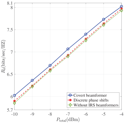
Figure 2:  $R_{\rm{b}}$ (bits/sec/Hz) versus $P_{\rm{total}}$ (dBW).

Fig. 2 investigates the covert rate of Bob $R_{\rm{b}}$ versus the total transmit power $P_{\rm{total}}$, where $K$=4. We can see that the covert rate of Bob $R_{\rm{b}}$ increases as the transmit power of Alice $P_{\rm{total}}$ increases. More specific, $R_{\rm{b}}$ of the covert beamforming design is the highest among the three design methods, while $R_{\rm{b}}$ of the without IRS design is the lowest. This is because that the reflected signal by the IRS and the direct signal can be better added constructively at Bob while destructively at Willie after continuously optimizing the IRS-related phase shifts.

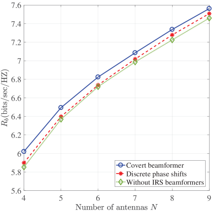
Figure 3: $R_{\rm{b}}$ versus the number of antennas $N$.

In Fig. 3, we plot the covert rate of Bob $R_{\rm{b}}$ versus the number of antennas of Alice $N$ with ${P_{{\rm{total}}}}=-10\rm{dBm}$ and $K$=4. It can be observed that for a fixed value of $N$, $R_{\rm{b}}$ of without IRS beamformer design is lower than that of the discrete phase shifts design, while $R_{\rm{b}}$ of the discrete phase shifts design is lower than that of the covert beamformer design, which is consistent with Fig. 2. Moreover, it can be seen that as the number of antennas $N$ increases, the covert rate of Bob $R_{\rm{b}}$ increases. This is because with more antennas, more spatial multiplexing gains can be exploited.

V-B Evaluation for Scenario 2

In this subsection, the proposed robust beamformer design for scenario that Alice with imperfect WCSI is evaluated.

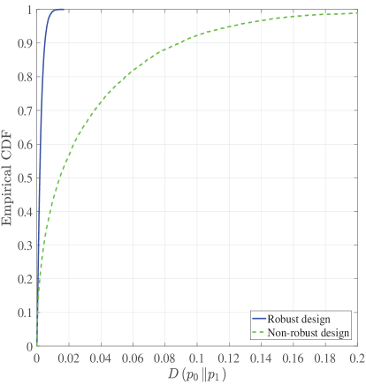
(a)

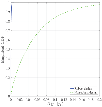
(b)

Figure 4: The empirical CDF of (a) $D\left({{p_{0}}\left\|{{p_{1}}}\right.}\right)$ and (b) $D\left({{p_{0}}\left\|{{p_{1}}}\right.}\right)$, with the covertness threshold $2{\varepsilon^{2}}=0.02$ and CSI error $v_{w}=0.0002$.

Fig. 4 (a) and (b) respectively show the empirical CDF of the achieved $D\left({{p_{0}}\left\|{{p_{1}}}\right.}\right)$ and $D\left({{p_{1}}\left\|{{p_{0}}}\right.}\right)$ when the CSI error parameter is $v_{w}={2}\times{{10}}^{{-4}}$. Here, the non-robust design refers to the proposed covert design with ${{{\bf{\hat{h}}}}_{\rm{IW}}}$ and ${{{\bf{\hat{h}}}}_{\rm{AW}}}$ under the same conditions. For both the robust and non-robust designs, the covertness threshold is $2{\varepsilon^{2}}=0.02$, i.e., $D\left({{p_{0}}\left\|{{p_{1}}}\right.}\right)\leq 0.02$ and $D\left({{p_{1}}\left\|{{p_{0}}}\right.}\right)\leq 0.02$. From the Fig. 4, the CDF in the KL divergence of the non-robust design does not satisfy the covert constraint. In addition, the robust beamforming design guarantees the requirement of the KL divergence. That is, it satisfies Willie’s error detection probability requirement. In general, Fig. 4 (a) and (b) verify the necessity and effectiveness of the proposed robust design.

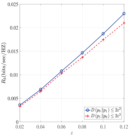
(a)

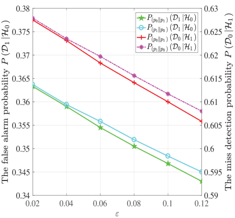
(b)

Figure 5: The value of $\varepsilon$ versus (a) the covert rate and (b) the detection error probabilities with CSI error $v_{w}={2}\times{10}^{-4}$.

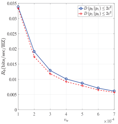
(a)

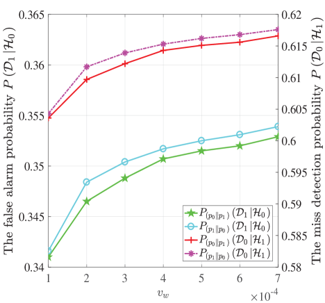
(b)

Figure 6: (a) The covert rate and (b) the detection error probabilities versus CSI error $v_{w}$ with the value of $\varepsilon=0.1$.

Fig. 5 (a) plots the covert rate $R_{\rm{b}}$ versus the value of $\varepsilon$ under two covertness constraints $D\left({{p_{0}}\left\|{{p_{1}}}\right.}\right)\leq 2{\varepsilon^{2}}$ and $D\left({{p_{1}}\left\|{{p_{0}}}\right.}\right)\leq 2{\varepsilon^{2}}$, where CSI error $v_{w}={2}\times{{10}}^{{-4}}$ and ${P_{{\rm{total}}}}=5\rm{dBm}$. Here, ${P_{\left({{p_{0}}\left\|{{p_{1}}}\right.}\right)}}\left({{{\cal D}_{1}}\left|{{{\cal H}_{0}}}\right.}\right)$ represents the false alarm probability $P\left({{{\cal D}_{1}}\left|{{{\cal H}_{0}}}\right.}\right)$ in the case of $D\left({{p_{0}}\left\|{{p_{1}}}\right.}\right)\leq 2{\varepsilon^{2}}$, and the other notation is defined likewise. This simulation result is consisted with the theoretical analysis. That is, when $\varepsilon$ becomes larger, the covertness constraint becomes loose, which leads to a larger $R_{\rm{b}}$. Fig. 5 (b) shows that the false alarm probability $P\left({{{\cal D}_{1}}\left|{{{\cal H}_{0}}}\right.}\right)$ and the missed detection probability $P\left({{{\cal D}_{0}}\left|{{{\cal H}_{1}}}\right.}\right)$ versus the value of $\varepsilon$ for CSI error $v_{w}={2}\times{{10}}^{{-4}}$. We observe that under both two different covert constraints, $P\left({{{\cal D}_{1}}\left|{{{\cal H}_{0}}}\right.}\right)$ and $P\left({{{\cal D}_{0}}\left|{{{\cal H}_{1}}}\right.}\right)$ are decreasing as $\varepsilon$ increases, where $P\left({{{\cal D}_{1}}\left|{{{\cal H}_{0}}}\right.}\right)$ is always lower than $P\left({{{\cal D}_{0}}\left|{{{\cal H}_{1}}}\right.}\right)$. It implies that when the convert constraint is looser, the detection performance of Willie becomes better. Moreover, Fig. 5 (b) also verifies the effectiveness of the proposed robust beamformers design in covert communications, that is, $\Pr\left({{{\cal D}_{1}}\left|{{{\cal H}_{0}}}\right.}\right)+\Pr\left({{{\cal D}_{0}}\left|{{{\cal H}_{1}}}\right.}\right)\geq 1-\varepsilon$. Therefore, from Fig. 5, we reveal the tradeoff between detection performance of Willie and covert rate of Bob, and a desired tradeoff can be achieved through an appropriate robust beamforming design.

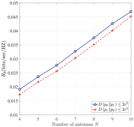
Figure 7: Covert rates $R_{\rm{b}}$ versus number of antennas $N$ with CSI error $v_{w}={2}\times{10}^{-4}$.

Fig. 6 (a) shows the covert rates $R_{\rm{b}}$ versus CSI error $v_{w}$ for the two KL divergence cases $D\left({{p_{0}}\left\|{{p_{1}}}\right.}\right)\leq 2{\varepsilon^{2}}$ and $D\left({{p_{1}}\left\|{{p_{0}}}\right.}\right)\leq 2{\varepsilon^{2}}$. From Fig. 6 (a), we can see that the higher the CSI error $v_{w}$ is, the lower the achieved covert rates $R_{\rm{b}}$ will be. Fig. 6 (b) shows the false alarm probability $P\left({{{\cal D}_{1}}\left|{{{\cal H}_{0}}}\right.}\right)$ and the missed detection probability $P\left({{{\cal D}_{0}}\left|{{{\cal H}_{1}}}\right.}\right)$ versus $v_{w}$ under two covertness constraints. We observe that under the two cases of covertness constraint, both the false alarm probability $P\left({{{\cal D}_{1}}\left|{{{\cal H}_{0}}}\right.}\right)$ and the missed detection probability $P\left({{{\cal D}_{0}}\left|{{{\cal H}_{1}}}\right.}\right)$ decrease when $v_{w}$ decreases, where $P\left({{{\cal D}_{1}}\left|{{{\cal H}_{0}}}\right.}\right)$ is always lower than $P\left({{{\cal D}_{0}}\left|{{{\cal H}_{1}}}\right.}\right)$. Moreover, Fig. 6 shows that a large error $v_{w}$ may cause a poor beamformer design in terms of cover rate $R_{\rm{b}}$. However, such beamformer may confuse Willie’s detection, which is also beneficial to Bob. Therefore, such a tradeoff also should be paid attention to the robust beamformer design.

Fig. 7 plots the covert rates $R_{\rm{b}}$ versus the number of antennas $N$ under two covertness constraints with ${P_{{\rm{total}}}}=5\rm{dBm}$, $\varepsilon=0.1$ and $v_{w}={2}\times{10}^{-4}$. It can be observed that as the number of antennas $N$ increase, the covert rates $R_{\rm{b}}$ of two covertness constraints increase, which is similar to the case in Fig. 7. From Fig. 5-7, we can see that the rates with the covertness constraint $D\left({{p_{0}}\left\|{{p_{1}}}\right.}\right)\leq 2{\varepsilon^{2}}$ are higher than those with two KL divergence cases $D\left({{p_{1}}\left\|{{p_{0}}}\right.}\right)\leq 2{\varepsilon^{2}}$. This is because $D\left({{p_{1}}\left\|{{p_{0}}}\right.}\right)\leq 2{\varepsilon^{2}}$ is stricter than $D\left({{p_{0}}\left\|{{p_{1}}}\right.}\right)\leq 2{\varepsilon^{2}}$, and this conclusion can also be found in [18].

VI Conclusions

In this paper, we designed both covert beamformer and robust beamformer for IRS assisted IoT networks, where Alice utilizes the IRS to covertly send a message to Bob to avoid being discovered by Willie. For the perfect WCSI scenario, we develop the covert beamformer design for the covert rate maximization, and the numerical results show that the covert beamformer design has better covert performance than the design without IRS. Furthermore, for practical imperfect WCSI scenario, we derived the covert decision threshold of Willie, the false alarm probability, and the missed detection probability. Then, by taking the impact of practical channel estimation errors into account, we proposed robust beamformers design, which can maximize the covert rate while meeting the covert requirements. Numerical results illustrated the validity of the proposed covert beamformers design and provided the useful insights on the effect of the main design parameters on the covert communication performance.

Appendix A Proof of the Proposition 1:

Let ${\bf{P}}$ denotes the projection matrix of vector ${{\bf{W}}_{\rm{b}}^{{1\mathord{\left/{\vphantom{12}}\right.\kern-1.2pt}2}}{\bf{t}}_{\rm{b}}^{H}}$, where ${\bf{W}}_{\rm{b}}$ is an SDR solution for problem (24),

$${\bf{P}}=\frac{{{\bf{W}}_{\rm{b}}^{{1\mathord{\left/{\vphantom{12}}\right.\kern-1.2pt}2}}{\bf{t}}_{\rm{b}}^{H}{{\left({{\bf{W}}_{\rm{b}}^{{1\mathord{\left/{\vphantom{12}}\right.\kern-1.2pt}2}}{\bf{t}}_{\rm{b}}^{H}}\right)}^{H}}}}{{{{\left\|{{\bf{t}}_{\rm{b}}^{H}{\bf{W}}_{\rm{b}}^{{1\mathord{\left/{\vphantom{12}}\right.\kern-1.2pt}2}}}\right\|}^{2}}}}=\frac{{{\bf{W}}_{\rm{b}}^{{1\mathord{\left/{\vphantom{12}}\right.\kern-1.2pt}2}}{\bf{t}}_{\rm{b}}^{H}{{\bf{t}}_{\rm{b}}}{\bf{W}}_{\rm{b}}^{{1\mathord{\left/{\vphantom{12}}\right.\kern-1.2pt}2}}}}{{{{\left({{\bf{W}}_{\rm{b}}^{{1\mathord{\left/{\vphantom{12}}\right.\kern-1.2pt}2}}{\bf{t}}_{\rm{b}}^{H}}\right)}^{H}}{\bf{W}}_{\rm{b}}^{{1\mathord{\left/{\vphantom{12}}\right.\kern-1.2pt}2}}{\bf{t}}_{\rm{b}}^{H}}},$$ (74)

We construct a new rank one solution ${{{\bf{\bar{W}}}}_{\rm{b}}}={\bf{W}}_{\rm{b}}^{{1\mathord{\left/{\vphantom{12}}\right.\kern-1.2pt}2}}{\bf{PW}}_{\rm{b}}^{{1\mathord{\left/{\vphantom{12}}\right.\kern-1.2pt}2}}$. Then, let us check the value of the objective function ${{\bf{W}}_{\rm{b}}}-{{{\bf{\bar{W}}}}_{\rm{b}}}{\rm{=}}{\bf{W}}_{\rm{b}}^{{1\mathord{\left/{\vphantom{12}}\right.\kern-1.2pt}2}}\left({{\bf{I}}-{\bf{P}}}\right){\bf{W}}_{\rm{b}}^{{1\mathord{\left/{\vphantom{12}}\right.\kern-1.2pt}2}}\underline{\succ}{\bf{0}}$. Thus, ${\rm{Tr}}\left({{{{\bf{\bar{W}}}}_{\rm{b}}}}\right)\leq{\rm{Tr}}\left({{{\bf{W}}_{\rm{b}}}}\right)\leq{P_{{\rm{total}}}}$, which means the solution ${{{\bf{\bar{W}}}}_{\rm{b}}}$ satisfies constraint (24c). Moreover, substituting ${{{\bf{\bar{W}}}}_{\rm{b}}}$ into the value of the objective function, we have

$${{\bf{t}}_{\rm{b}}}{{{\bf{\bar{W}}}}_{\rm{b}}}{\bf{t}}_{\rm{b}}^{H} ={{\bf{t}}_{\rm{b}}}{\bf{W}}_{\rm{b}}^{{1\mathord{\left/{\vphantom{12}}\right.\kern-1.2pt}2}}{\bf{PW}}_{\rm{b}}^{{1\mathord{\left/{\vphantom{12}}\right.\kern-1.2pt}2}}{\bf{t}}_{\rm{b}}^{H}$$

$$=\frac{{{{\bf{t}}_{\rm{b}}}{\bf{W}}_{\rm{b}}^{{1\mathord{\left/{\vphantom{12}}\right.\kern-1.2pt}2}}{\bf{W}}_{\rm{b}}^{{1\mathord{\left/{\vphantom{12}}\right.\kern-1.2pt}2}}{\bf{t}}_{\rm{b}}^{H}{{\bf{t}}_{\rm{b}}}{\bf{W}}_{\rm{b}}^{{1\mathord{\left/{\vphantom{12}}\right.\kern-1.2pt}2}}{\bf{W}}_{\rm{b}}^{{1\mathord{\left/{\vphantom{12}}\right.\kern-1.2pt}2}}{\bf{t}}_{\rm{b}}^{H}}}{{{{\left({{\bf{W}}_{\rm{b}}^{{1\mathord{\left/{\vphantom{12}}\right.\kern-1.2pt}2}}{\bf{t}}_{\rm{b}}^{H}}\right)}^{H}}{\bf{W}}_{\rm{b}}^{{1\mathord{\left/{\vphantom{12}}\right.\kern-1.2pt}2}}{\bf{t}}_{\rm{b}}^{H}}}$$

$$={{\bf{t}}_{\rm{b}}}{{\bf{W}}_{\rm{b}}}{\bf{t}}_{\rm{b}}^{H}.$$ (75)

Hence, the value of the objective function remains the same ${\bf{W}}_{\rm{b}}$ is replaced with ${{{\bf{\bar{W}}}}_{\rm{b}}}$. Finally, let us check whether the constraint (24b) is satisfied for the new solution ${{{\bf{\bar{W}}}}_{\rm{b}}}$

$${{\bf{t}}_{\rm{w}}}{{\bf{W}}_{\rm{b}}}{\bf{t}}_{\rm{w}}^{H}-{{\bf{t}}_{\rm{w}}}{{{\bf{\bar{W}}}}_{\rm{b}}}{\bf{t}}_{\rm{w}}^{H} ={{\bf{t}}_{\rm{w}}}\left({{{\bf{W}}_{\rm{b}}}-{\bf{W}}_{\rm{b}}^{{1\mathord{\left/{\vphantom{12}}\right.\kern-1.2pt}2}}{\bf{PW}}_{\rm{b}}^{{1\mathord{\left/{\vphantom{12}}\right.\kern-1.2pt}2}}}\right){\bf{t}}_{\rm{w}}^{H}$$

$$={{\bf{t}}_{\rm{w}}}\left({{\bf{W}}_{\rm{b}}^{{1\mathord{\left/{\vphantom{12}}\right.\kern-1.2pt}2}}\left({{\bf{I}}-{\bf{P}}}\right){\bf{W}}_{\rm{b}}^{{1\mathord{\left/{\vphantom{12}}\right.\kern-1.2pt}2}}}\right){\bf{t}}_{\rm{w}}^{H}$$

$$\geq{\rm{0}}.$$ (76)

Due to the value of the ${\rm{Tr}}\left({{{\bf{t}}_{\rm{w}}}{{\bf{W}}_{\rm{b}}}{\bf{t}}_{\rm{w}}^{H}}\right){\rm{=0}}$, thus, ${\rm{Tr}}\left({{{\bf{t}}_{\rm{w}}}{{{\bf{\bar{W}}}}_{\rm{b}}}{\bf{t}}_{\rm{w}}^{H}}\right){\rm{=0}}$.

References

[1]
S. Gong, X. Lu, D. T. Hoang, D. Niyato, L. Shu, D. I. Kim, and
Y. C. Liang,
“Toward smart wireless communications via intelligent reflecting
surfaces: A contemporary survey,”
IEEE Commun. Surv. Tutor., vol. 22, no. 4, pp. 2283–2314, Jun.
2020.
[2]
W. Guo, H. Zhang, and C. Huang,
“Energy efficiency of two-way communications under various duplex
modes,”
IEEE Internet Thing J., vol. 8, no. 3, pp. 1921–1933, Feb.
2020.
[3]
Q. Wu and R. Zhang,
“Towards smart and reconfigurable environment: Intelligent
reflecting surface aided wireless network,”
IEEE Commun. Magazine, vol. 58, no. 1, pp. 106–112, Jan. 2020.
[4]
X. Tan, Z. Sun, J. M. Jornet, and D. Pados,
“Increasing indoor spectrum sharing capacity using smart
reflect-array,”
in Proc. 2016 IEEE International Conference on Communications
(ICC), pp. 1–6, 2016.
[5]
G. Yu, X. Chen, C. Zhong, D. W. Kwan Ng, and Z. Zhang,
“Design, analysis, and optimization of a large intelligent
reflecting surface-aided B5G cellular internet of things,”
IEEE Internet Things J., vol. 7, no. 9, pp. 8902–8916, Sept.
2020.
[6]
M. Cui, G. Zhang, and R. Zhang,
“Secure wireless communication via intelligent reflecting surface,”
IEEE Wireless Commun. Lett., vol. 8, no. 5, pp. 1410–1414,
Oct. 2019.
[7]
L. Dong and H. Wang,
“Secure MIMO transmission via intelligent reflecting surface,”
IEEE Wireless Commun. Lett., vol. 9, no. 6, pp. 787–790, Jun.
2020.
[8]
X. Yu, D. Xu, Y. Sun, D. W. K. Ng, and R. Schober,
“Robust and secure wireless communications via intelligent
reflecting surfaces,”
IEEE J. Sel. Areas Commun., vol. 38, no. 11, pp. 2637–2652,
Nov. 2020.
[9]
S. Hong, C. Pan, H. Ren, K. Wang, and A. Nallanathan,
“Artificial-noise-aided secure MIMO wireless communications via
intelligent reflecting surface,”
IEEE Trans. Commun., vol. 68, no. 12, pp. 7851–7866, Dec.
2020.
[10]
Z. Chu, W. Hao, P. Xiao, D. Mi, Z. Liu, M. Khalily, J. R. Kelly,
and A. P. Feresidis,
“Secrecy rate optimization for intelligent reflecting surface
assisted MIMO system,”
IEEE Trans. Inf. Forensics Security, vol. 16, no. 18,
pp. 1655–1669, Nov. 2021.
[11]
M. Bloch and J. Barros,
Physical-Layer Security: From Information Theory to Security
Engineering,
U.K.: Cambridge Univ., 2011.
[12]
X. Lu, E. Hossain, T. Shafique, S. Feng, H. Jiang, and D. Niyato,
“Intelligent reflecting surface enabled covert communications in
wireless networks,”
IEEE Netw., vol. 34, no. 5, pp. 148–155, Oct. 2020.
[13]
J. Si, Z. Li, Y. Zhao, J. Cheng, L. Guan, J. Shi, and N. AL-Dhahir,
“Covert transmission assisted by intelligent reflecting surface,”
arXiv:2008.05031, Jan. 2021.
[14]
X. Zhou, S. Yan, Q. Wu, F. Shu, and D. W. K. Ng,
“Intelligent reflecting surface (IRS)-aided covert wireless
communication with delay constraint,”
arXiv:2011.03726., Nov. 2020.
[15]
C. Wang, Z. Li, J. Shi, and D. W. K. Ng,
“Intelligent reflecting surface-assisted multi-antenna covert
communications: Joint active and passive beamforming optimization,”
IEEE Trans. Commun., 2021.
[16]
L. Lv, Q. Wu, Z. Li, Z. Ding, N. AL-Dhahir, and J. Cheng,
“Covert communication in intelligent reflecting surface-assisted
NOMA systems: Design, analysis, and optimization,”
arXiv:2012.03244, Dec. 2020.
[17]
E. L. Lehmann and J. P. Romano,
Testing Statistical Hypotheses,
Springer New York, 2005.
[18]
S. Yan, Y. Cong, S. V. Hanly, and X. Zhou,
“Gaussian signalling for covert communications,”
IEEE Trans. Wireless Commun., vol. 18, no. 7, pp. 3542–3553,
Jul. 2019.
[19]
T. M. Cover and J. A. Thomas,
Elements of Information Theory,
New York:Wiley, 2006.
[20]
B. A. Bash, D. Goeckel, and D. Towsley,
“Limits of reliable communication with low probability of detection
on AWGN channels,”
IEEE J. Sel. Areas Commun., vol. 31, no. 9, pp. 1921–1930,
Sept. 2013.
[21]
M. Forouzesh, P. Azmi, N. Mokari, and D. Goeckel,
“Covert communication using null space and 3D beamforming:
Uncertainty of willie’s location information,”
IEEE Trans. Veh. Technol., vol. 69, no. 8, pp. 8568–8576, Aug.
2020.
[22]
Z. Luo, W. Ma, A. M. So, Y. Ye, and S. Zhang,
“Semidefinite relaxation of quadratic optimization problems,”
IEEE Signal Process. Mag., vol. 27, no. 3, pp. 20–34, May.
2010.
[23]
M. Grant and S. Boyd,
“CVX: Matlab software for disciplined convex programming, version
2.1,” http://cvxr.com/cvx, Mar. 2014.
[24]
Q. Wu and R. Zhang,
“Beamforming optimization for intelligent reflecting surface with
discrete phase shifts,”
in 2019 IEEE International Conference on Acoustics, Speech and
Signal Processing (ICASSP), pp. 7830–7833, Apr. 2019.
[25]
D. Goeckel, B. Bash, S. Guha, and D. Towsley,
“Covert communications when the warden does not know the background
noise power,”
IEEE Commun. Lett., vol. 20, no. 2, pp. 236–239, Feb. 2016.
[26]
K. Shahzad, X. Zhou, and S. Yan,
“Covert communication in fading channels under channel
uncertainty,”
in Proc. IEEE VTC Spring, pp. 1–5, Jun. 2017.
[27]
M. Zheng, A. Hamilton, and C. Ling,
“Covert communications with a full-duplex receiver in non-coherent
rayleigh fading,”
IEEE Trans. Commun., vol. 69, no. 3, pp. 1882–1895, Mar. 2021.
[28]
M. Forouzesh, P. Azmi, N. Mokari, and D. Goeckel,
“Robust power allocation in covert communication: Imperfect CDI,”
arXiv:1901.04914., Jan. 2019.
[29]
G. Zhou, C. Pan, H. Ren, K. Wang, M. D. Renzo, and A. Nallanathan,
“Robust beamforming design for intelligent reflecting surface aided
MISO communication systems,”
IEEE Wireless Commun. Lett., vol. 9, no. 10, pp. 1658–1662,
Oct. 2020.
[30]
L. Wang, W. Wornell, and L. Zheng,
“Fundamental limits of communication with low probability of
detection,”
IEEE Trans. Inf. Theory, vol. 62, no. 6, pp. 3493–3503, Jun.
2016.
[31]
M. R. Bloch,
“Covert communication over noisy channels: A resolvability
perspective,”
IEEE Trans. Inf. Theory, vol. 62, no. 5, pp. 2334–2354, May.
2016.
[32]
D. W. K. Ng, E. S. Lo, and R. Schober,
“Robust beamforming for secure communication in systems with
wireless information and power transfer,”
IEEE Trans. Wireless Commun., vol. 13, no. 8, pp. 4599–4615,
Aug. 2014.