Matching Theory and Evidence on Covid-19 using a Stochastic Network SIR Model

Abstract

This paper develops an individual-based stochastic network SIR model for the empirical analysis of the Covid-19 pandemic. It derives moment conditions for the number of infected and active cases for single as well as multigroup epidemic models. These moment conditions are used to investigate the identification and estimation of the transmission rates. The paper then proposes a method that jointly estimates the transmission rate and the magnitude of under-reporting of infected cases. Empirical evidence on six European countries matches the simulated outcomes once the under-reporting of infected cases is addressed. It is estimated that the number of actual cases could be between 4 to 10 times higher than the reported numbers in October 2020 and declined to 2 to 3 times in April 2021. The calibrated models are used in the counterfactual analyses of the impact of social distancing and vaccination on the epidemic evolution, and the timing of early interventions in the UK and Germany.

Keywords: Covid-19, multigroup SIR model, basic and effective reproduction numbers, transmission rates, vaccination, calibration and counterfactual analysis.

JEL Classifications: C13, C15, C31, D85, I18, J18

1 Introduction

Since the outbreak of Covid-19, many researchers in epidemiology, behavioral sciences, and economics have applied various forms of compartmental models to study the disease transmission and potential outcomes under different intervention policies. The compartmental models are a major group of epidemiological models that categorize a population into several types or groups, such as susceptible (S), infected (I), and removed (recovered or deceased, R). Compartmental models owe their origin to the well-known SIR model pioneered by Kermack and McKendrick (1927) and have been developed in a number of important directions, allowing for multi-category (multi-location), under a variety of contact networks and transmission channels.

In this paper, we develop a new stochastic network SIR model in which individual-specific infection and recovery processes are modelled, allowing for group heterogeneity and latent individual characteristics that distinguish individuals in terms of their degrees of resilience to becoming infected. The model is then used to derive individual-specific conditional probabilities of infection and recovery. In this respect, our modelling approach is to be distinguished from the individual-based models in epidemiology that specify the transition probabilities of individuals from one state to another. In modelling the infection process, we consider an individual’s contact pattern with others in the network, plus an individual-specific latent factor assumed to be exponentially distributed. The time from infection to recovery (or death) is assumed to be geometrically distributed. The individual processes are shown to aggregate up to the familiar multigroup SIR model. We allow for group heterogeneity and, in line with the literature, assume contact probabilities are homogeneous within groups but could differ across groups.

We then derive the probabilities of individuals within a given group being in a particular state at a given time, conditional on contact patterns, exposure intensities, and unobserved characteristics. These conditional probabilities are aggregated up to form a set of moment conditions that can be taken to the data on the number of infected and active cases both at the aggregate and group (or regional) levels. We make use of the moment conditions to investigate the identification of the underlying structural parameters. Most importantly, we show that whilst one cannot distinguish between average contact numbers and the degree of exposure to the virus upon contact, it is nevertheless possible to identify the basic and effective reproduction numbers from relatively short time series observations on infections and recoveries. Using Monte Carlo simulations, the small sample properties of the proposed estimator are shown to be satisfactory, with a high degree of precision even when using two and three weeks of rolling observations.

However, in practice, estimation of the transmission rate must take account of the well-known measurement problem where the number of infected cases is often grossly under-reported. This problem is further complicated since the degree of under-reporting varies over time and tends to fall as society becomes more familiar with the disease and testing becomes more widespread. To deal with this mismeasurement problem, we propose a new method that jointly estimates the transmission rates and the multiplication factor that measures the degree of under-reporting. Equipped with daily estimates of the transmission rates, we are then able to calibrate our epidemic model and investigate its properties under different network topology, group numbers, and different social distancing and vaccination strategies.

We apply the proposed joint estimation approach to examine how well the outcome of the proposed epidemic model matches the Covid-19 evidence in the case of six European countries (Austria, France, Germany, Italy, Spain, and the UK) from March 2020 to April 2021. We provide rolling estimates of the transmission rates and related effective reproduction numbers, as well as estimates of multiple factors. We then use the estimated transmission rates to calibrate the model parameters across the six countries. The stochastically simulated outcomes are shown to be reasonably close to the reported cases once the under-reporting issue has been addressed. We estimate that the degree of under-reporting declined from a multiple of $4$–$10$ to $2$–$3$ times during the study period across the countries considered.

Finally, we illustrate the use of our model for two different counterfactual exercises. First, we consider the effects of vaccination on the evolution of the epidemic using a multigroup setup, where we also evaluate the implications of age-based vaccine prioritization on the outcomes. Our model allows each individual to have their own degree of immunity, with vaccination increasing this individual-specific immunity by a factor of $20$ in the case of Moderna or Pfizer-BioNTech that are shown to be $94$–$95\%$ effective (Oliver et al., 2020, 2021). The multigroup model is particularly helpful in examining the implications of different vaccine prioritization strategies. Second, we investigate the potential outcomes if the first lockdown in Germany had been delayed for one or two weeks; and if the lockdown in the UK had started one or two weeks earlier. Such counterfactual analyses can be achieved by shifting the estimated transmission rates forward or backward. We show that early intervention is critical in managing the infection and controlling the total number of infected and active cases.

The problem of how to balance the public health risks from the spread of the epidemic with the economic costs associated with lockdowns and other mandatory social-distancing regulations will not be addressed in this paper. However, the proposed network SIR model with its individual-based architecture is eminently suited to this purpose. The proposed model can be combined with behavioral assumptions about how individuals trade off infection risk and economic well-being, thus generalizing the aggregate framework proposed in Chudik, Pesaran, and Rebucci (2021) to individual-based SIR models.

The rest of the paper is organized as follows. Section 2 introduces the basic concepts and the classical multigroup SIR model. Section 3 lays out our individual based stochastic model on a network. Section 4 explains the calibration of our model to basic and effective reproduction numbers. Section 5 documents the properties of the model. Sections 6 discusses the estimation of the transmission rate. Section 7 presents the calibration of the model to Covid-19 evidence. Section 8 concentrates on the counterfactual analyses, and Section 9 concludes.

To save space, a detailed review of the related literature is given in an online supplement, where we also provide supplementary theoretical derivations, additional estimation results, counterfactual outcomes, and data sources.

2 Basic concepts and the multigroup SIR model

We consider a population of $n$ individuals susceptible to the spread of a disease with some initially infected individuals. We suppose that the susceptible population can be categorized into $L$ groups of size $n_{\ell}$, $\ell=1,2,\ldots,L$, with $L$ fixed such that $n=\sum_{\ell=1}^{L}n_{\ell}$. It is further assumed that the group shares, $w_{\ell}=n_{\ell}/n>0,$ for all $n$ and as $n\rightarrow\infty$. The grouping could be based on demographic factors (age and/or gender), or other observed characteristics such as contact locations and/or schedules, mode of transmission, genetic susceptibility, group-specific vaccination coverage, as well as socioeconomic factors (see, e.g., Hethcote, 2000). Individual $i$ in group $\ell$ will be referred to as individual $\left(i,\ell\right)$, with $i=1,2,\ldots,n_{\ell}$ and $\ell=1,2,\ldots,L$. It is assumed that $n_{\ell}$ is relatively large but remains fixed over the course of the epidemic measured in days.

Suppose that individual $\left(i,\ell\right)$ becomes infected on day $t=t_{i\ell}^{\ast}$, and let $x_{i\ell,t}$ take the value of unity for all $t\geq t_{i\ell}^{\ast}$, and zero otherwise. In this way, we follow the convention that once an individual becomes infected, he/she is considered as infected thereafter, irrespective of whether that individual recovers or dies. Specifically, we set

$$x_{i\ell,t}=0,\text{ for all }t<t_{i\ell}^{\ast};\text{ \ and \ }x_{i\ell,t}=1,\text{ for all }t\geq t_{i\ell}^{\ast}.$$ (1)

The event of recovery or death of individual $\left(i,\ell\right)$ at time $t$ will be represented by $y_{i\ell,t}$, which will be equal to zero unless the individual is ”removed” (recovered or dead). An individual $(i,\ell)$ is considered to be ”active” if he/she is infected and not yet recovered. We denote the active indicator by $z_{i\ell,t},$ which is formally defined by

$$z_{i\ell,t}=\left(1-y_{i\ell,t}\right)x_{i\ell,t}.$$ (2)

$z_{i\ell,t}$ takes the value of $0$ if individual $(i,\ell)$ has not been infected, or has been infected but recovered/dead. It takes the value of $1$ if he/she is infected and not yet recovered. Any individual $(i,\ell)$ who has not been infected is viewed ”susceptible” and indicated by $s_{i\ell,t}=1$, where

$$s_{i\ell,t}=1-z_{i\ell,t}-y_{i\ell,t}.$$ (3)

It then readily follows that the total (cumulative) number of those ”infected” in group $\ell$ at the end of day $t$ is given by

$$C_{\ell t}=\sum_{i=1}^{n_{\ell}}x_{i\ell,t},\text{ }\ell=1,2,\ldots,L,$$ (4)

where the summation is over all individuals in group $\ell$. The total number of ”recovered” in group $\ell$ in day $t$ is given by

$$R_{\ell t}=\sum_{i=1}^{n_{\ell}}y_{i\ell,t},\text{ }\ell=1,2,\ldots,L.$$ (5)

The total number of ”active” cases (individuals who are infected and not yet removed) in group $\ell$ in day $t$ is

$$I_{\ell t}=\sum_{i=1}^{n_{\ell}}z_{i\ell,t}=\sum_{i=1}^{n_{\ell}}x_{i\ell,t}-\sum_{i=1}^{n_{\ell}}x_{i\ell,t}y_{i\ell,t}=C_{\ell t}-R_{\ell t}.$$ (6)

The number of ”susceptible” individuals in group $\ell$ in day $t$ is

$$S_{\ell t}=\sum_{i=1}^{n_{\ell}}s_{i\ell,t}=n_{\ell}-I_{\ell t}-R_{\ell t}\text{.}$$ (7)

Our model does not distinguish between recovery and death. Once an individual is removed (recovered or dead), following the SIR literature, we assume that he/she cannot be infected again. Under this assumption, recovery and death have the same effects on the evolution of the epidemic, and accordingly in what follows we shall not differentiate between recovery and death and refer to their total as ”removed”.

The classic multigroup SIR model in discretized form can be written as

$$S_{\ell,t+1}-S_{\ell t} =-S_{\ell t}\sum_{\ell^{{}^{\prime}}=1}^{L}\beta_{\ell\ell^{\prime}}I_{\ell^{{}^{\prime}}t},$$ (8)

$$I_{\ell,t+1}-I_{\ell t} =S_{\ell t}\sum_{\ell^{{}^{\prime}}=1}^{L}\beta_{\ell\ell^{\prime}}I_{\ell^{{}^{\prime}}t}-\gamma_{\ell}I_{\ell t}$$ (9)

$$R_{\ell,t+1}-R_{\ell t} =\gamma_{\ell}I_{\ell t},$$ (10)

for $\ell=1,2,\ldots,L$ and $t=1,2,\ldots,T$, where $S_{\ell t}$, $I_{\ell t}$ and $R_{\ell t}$ are defined as above, $\gamma_{\ell}$ is the recovery rate which is assumed to be time-invariant and the same for all people in group $\ell$, and $\beta_{\ell\ell^{\prime}}$ is the transmission coefficient between $S_{\ell t}$ and $I_{\ell^{{}^{\prime}}t}$. Note that individuals in group $\ell^{{}^{\prime}}$ may transmit the disease to individuals in group $\ell$, with the new infections in group $\ell$ given by $S_{\ell t}\sum_{\ell^{{}^{\prime}}=1}^{L}\beta_{\ell\ell^{\prime}}I_{\ell^{{}^{\prime}}t}$.

3 An individual based stochastic epidemic model on a network

We now depart from the literature by explicitly modelling the individual indicators, $x_{i\ell,t}$ and $y_{i\ell,t}$, (and hence $z_{i\ell,t}$) and then simulate and aggregate up to match the theoretical predictions with realized aggregated outcomes. In this section, we first describe the infection and recovery processes at the individual level, we then show how they lead to the moment conditions at group levels, and finally derive the relation between aggregated outcomes from our model and the multigroup SIR deterministic model.

3.1 Modelling the infection and recovery processes

As an attempt to better integrate individual decisions to mitigate their health risk within the epidemic model, we propose to directly model $x_{i\ell,t}$ for each individual $(i,\ell)$, as compared to modelling the group aggregates $S_{\ell t}$, $R_{\ell t}$, and $I_{\ell t}$. We follow the micro-econometric literature and model the infection process using the latent variable, $x_{i\ell,t+1}^{\ast},$ which determines whether individual $(i,\ell)$ becomes infected. Specifically, we begin with the following Markov switching process for individual $(i,\ell)$:

$$x_{i\ell,t+1}=x_{i\ell,t}+\left(1-x_{i\ell,t}\right)I\left(x_{i\ell,t+1}^{\ast}>0\right),$$ (11)

where $I\left(\mathcal{A}\right)$ is the indicator function that takes the value of unity if $\mathcal{A}$ holds and zero otherwise. We suppose that $x_{i\ell,t+1}^{\ast}$ is composed of two different components. The first component relates to the contact pattern of individual $(i,\ell)$ with all other individuals in the active set, denoted by $z_{j\ell^{\prime},t},$ both within (when $\ell^{\prime}=\ell$) and outside of his/her group (when $\ell^{\prime}\neq\ell$). The second component is an unobserved individual-specific infection threshold variable, $\xi_{i\ell,t+1}>0$. Formally, we set

$$x_{i\ell,t+1}^{\ast}=\tau_{i\ell}\sum_{\ell^{{}^{\prime}}=1}^{L}\sum_{j=1}^{n_{\ell^{{}^{\prime}}}}d_{i\ell,j\ell^{{}^{\prime}}}\left(t\right)z_{j\ell^{\prime},t}-\xi_{i\ell,t+1},$$ (12)

where the first component depends on the pattern of contacts, $d_{i\ell,j\ell^{{}^{\prime}}}\left(t\right)$, whether the contacted individuals are infectious, $z_{j\ell^{{}^{\prime}},t}$, and the exposure intensity parameter, denoted by $\tau_{i\ell}$. $\mathbf{D}(t)=\left[d_{i\ell,j\ell^{{}^{\prime}}}\left(t\right)\right]$ is the contact network matrix, such that $d_{i\ell,j\ell^{{}^{\prime}}}\left(t\right)=1$ if individual $\left(i,\ell\right)$ is in contact with individual $\left(j,\ell^{{}^{\prime}}\right)$ at time $t.$ $z_{j\ell^{\prime},t}=\left(1-y_{j\ell^{\prime},t}\right)x_{j\ell^{\prime},t}$ is an infectious indicator, already defined by (2), and takes the value of unity if individual $\left(j,\ell^{\prime}\right)$ is infected and not yet recovered, zero otherwise. The exposure intensity parameter, $\tau_{i\ell}$, is group-specific and depends on the average duration of contacts, whether the contacting individuals are wearing facemasks, and if they follow other recommended precautions.

The multigroup structure of the first component of (12) covers a wide range of observable characteristics, and can be extended to allow for differences in age, location, and medical pre-conditions. There are also many unobservable characteristics that lead to different probabilities of infection, even for individuals with the same contact patterns and exposure intensities. To allow for such latent factors, we have introduced the individual-specific positive random variable ($\xi_{i\ell,t+1}>0$) which represents the individual’s degree of resilience to becoming infected and varies across $(i,\ell)$ and $t.$ Ceteris paribus, an individual with a low value of $\xi_{i\ell,t+1}$ is more likely to become infected. $\xi_{i\ell,t+1}$ is assumed to be independently distributed over $i$, $\ell$ and $t$, and follows an exponential distribution with the cumulative distribution function given by

$$\Pr\left(\xi_{i\ell,t+1}<a\right)=1-\exp\left(-\mu_{i\ell}^{-1}a\right),\text{ \ for }a>0,$$ (13)

where $\mu_{i\ell}=E\left(\xi_{i\ell,t+1}\right)$.

To complete the specification of the infection process we also need to model $y_{i\ell,t}$, namely the recovery indicator. We assume that recovery depends on the number of days since infection. Specifically, the recovery process for individual $i$ is defined by

$$y_{i\ell,t+1}=y_{i\ell,t}+z_{i\ell,t}\text{ }\zeta_{i\ell,t+1}\left(t_{i\ell}^{\ast}\right),$$ (14)

where $z_{i\ell,t}=\left(1-y_{i\ell,t}\right)x_{i\ell,t}$, $\zeta_{i\ell,t+1}\left(t_{i\ell}^{\ast}\right)=1$ if individual $\left(i,\ell\right)$ recovers at time $t+1$, having been infected exactly at time $t_{i\ell}^{\ast}$ and not before, and $\zeta_{i\ell,t+1}\left(t_{i\ell}^{\ast}\right)=0,$ otherwise. The analysis of recovery simplifies considerably if we assume time to removal, denoted by $T_{i\ell,t}^{\ast}=t-t_{i\ell}^{\ast},$ follows the geometric distribution (for $t-t_{i\ell}^{\ast}=1,2,\ldots$)

$$\Pr\left[\zeta_{i\ell,t+1}\left(t_{i\ell}^{\ast}\right)=1\right]=\Pr\left(T_{i\ell,t}^{\ast}=t-t_{i\ell}^{\ast}\right)=\gamma_{\ell}\left(1-\gamma_{\ell}\right)^{t-t_{i\ell}^{\ast}-1}.$$ (15)

Then the probability of recovery at time $t+1$ having remained infected for $t-t_{i\ell}^{\ast}-1$ days (also known as the ”hazard function”) is given by

$$E\left[\zeta_{i\ell,t+1}\left(t_{i\ell}^{\ast}\right)\left|x_{i\ell,t},y_{i\ell,t},y_{i\ell,t-1},\ldots,y_{i\ell,t_{i\ell}^{\ast}}\right.\right]=\frac{\Pr\left(T_{i\ell,t}^{\ast}=t-t_{i\ell}^{\ast}\right)}{\Pr\left(T_{i\ell,t}^{\ast}>t-t_{i\ell}^{\ast}-1\right)}=\gamma_{\ell},$$ (16)

which is the same across all individuals within a given group and, most importantly, does not depend on the number of days since infection. Therefore, using (16) in (14), the recovery micro-moment condition simplifies to

$$E\left(y_{i\ell,t+1}\left|y_{i\ell,t},z_{i\ell,t}\right.\right)=y_{i\ell,t}+\gamma_{\ell}z_{i\ell,t}\text{,}$$ (17)

which implies that

$$E\left(y_{i\ell,t+1}\left|\mathbf{y}_{\ell,t},\mathbf{z}_{\ell,t}\right.\right)=y_{i\ell,t}+\gamma_{\ell}z_{i\ell,t}\text{,}$$ (18)

where $\mathbf{y}_{\ell,t}=(y_{1\ell,t},y_{2\ell,t},....,y_{n_{\ell}\ell,t})^{\prime}$ and $\mathbf{z}_{\ell,t}=(z_{1\ell,t},z_{2\ell,t},....,z_{n_{\ell}\ell,t})^{\prime}.$

We assume that $d_{i\ell,j\ell^{{}^{\prime}}}\left(t\right)$, the elements of the $n\times n$ network matrix $\mathbf{D}\left(t\right)=\left[d_{i\ell,j\ell^{{}^{\prime}}}\left(t\right)\right],$ are independent draws with $E\left[d_{i\ell,j\ell^{{}^{\prime}}}\left(t\right)\right]=p_{\ell\ell^{{}^{\prime}}}$, namely, the probability of contacts is homogeneous within groups but differs across groups. Let $\boldsymbol{d}_{i}^{{}^{\prime}}\left(t\right)$ be the $i^{th}$ row of $\mathbf{D}\left(t\right)$. Also let $\mathbf{z}_{t}$ be a column vector consisting of $z_{j\ell,t}$, for $j=1,2,\ldots,n_{\ell}$ and $\ell=1,2,\ldots,L$. Then using (11) we have

$$E\left[x_{i\ell,t+1}|x_{i\ell,t},\mathbf{z}_{t},\boldsymbol{d}_{i}\left(t\right),\tau_{i\ell},\mu_{i\ell}\right] =x_{i\ell,t}+\left(1-x_{i\ell,t}\right)\Pr\left[x_{i\ell,t+1}^{\ast}>0|\text{ }\mathbf{z}_{t}\text{, }\boldsymbol{d}_{i}\left(t\right)\right]$$

$$=x_{i\ell,t}+\left(1-x_{i\ell,t}\right)\Pr\left[\xi_{i\ell,t+1}<\tau_{i\ell}\sum_{\ell^{{}^{\prime}}=1}^{L}\sum_{j=1}^{n_{\ell^{{}^{\prime}}}}d_{i\ell,j\ell^{{}^{\prime}}}\left(t\right)z_{j\ell^{{}^{\prime}},t}\right]$$

$$=x_{i\ell,t}+\left(1-x_{i\ell,t}\right)\left\{1-\exp\left[-\theta_{i\ell}\sum_{\ell^{{}^{\prime}}=1}^{L}\sum_{j=1}^{n_{\ell^{{}^{\prime}}}}d_{i\ell,j\ell^{{}^{\prime}}}\left(t\right)z_{j\ell^{{}^{\prime}},t}\right]\right\},$$

where $\theta_{i\ell}=\tau_{i\ell}/\mu_{i\ell}$, which represents the net exposure effect. Since in general individual contact patterns are not observed, we also need to derive $E\left(x_{i\ell,t+1}|x_{i\ell,t},\mathbf{z}_{t},\theta_{i\ell}\right)$. To this end, we first note that

$$E\left\{\exp\left[-\theta_{i\ell}d_{i\ell,j\ell^{{}^{\prime}}}\left(t\right)z_{j\ell^{{}^{\prime}},t}\right]|\text{ }\mathbf{z}_{t},\theta_{i\ell}\right\} =\Pr\left[d_{i\ell,j\ell^{{}^{\prime}}}\left(t\right)=0\right]+\exp\left(-\theta_{i\ell}z_{j\ell^{{}^{\prime}},t}\right)\Pr\left[d_{i\ell,j\ell^{{}^{\prime}}}\left(t\right)=1\right]$$

$$=\left(1-p_{\ell\ell^{{}^{\prime}}}\right)+\exp\left(-\theta_{i\ell}z_{j\ell^{{}^{\prime}},t}\right)p_{\ell\ell^{{}^{\prime}}},$$

and since by assumption $d_{i\ell,j\ell^{{}^{\prime}}}\left(t\right)$ are independently distributed, we then have

$$E\left(x_{i\ell,t+1}|x_{i\ell,t},\mathbf{z}_{t},\theta_{i\ell}\right) =x_{i\ell,t}+\left(1-x_{i\ell,t}\right)\left\{1-E\left[\exp\left(-\theta_{i\ell}\sum_{\ell^{{}^{\prime}}=1}^{L}\sum_{j=1}^{n_{\ell^{\prime}}}d_{i\ell,j\ell^{{}^{\prime}}}\left(t\right)z_{j\ell^{{}^{\prime}},t}\right)\right]\right\}$$

$$=1-\left(1-x_{i\ell,t}\right)\prod_{\ell^{{}^{\prime}}=1}^{L}\prod_{j=1}^{n_{\ell^{\prime}}}\left[1-p_{\ell\ell^{{}^{\prime}}}+\exp\left(-\theta_{i\ell}z_{j\ell^{{}^{\prime}},t}\right)p_{\ell\ell^{{}^{\prime}}}\right].$$

However, recall that $z_{j\ell^{\prime},t}=1$ if individual $\left(j,\ell^{\prime}\right)$ is currently infected (namely if at time $t$ he/she is a member of the active set, $\mathcal{I}_{t}$), otherwise $z_{j\ell^{\prime},t}=0$. In the latter case $1-p_{\ell\ell^{{}^{\prime}}}+\exp\left(-\theta_{i\ell}z_{j\ell^{{}^{\prime}},t}\right)p_{\ell\ell^{{}^{\prime}}}=1$, and hence

$$E\left(x_{i\ell,t+1}|x_{i\ell,t},\mathbf{z}_{t},\theta_{i\ell}\right) =1-\left(1-x_{i\ell,t}\right)\prod_{\ell^{{}^{\prime}}=1}^{L}\left[\prod_{j=1,z_{j\ell^{\prime},t}=1}^{n_{\ell^{\prime}}}\left(1-p_{\ell\ell^{{}^{\prime}}}+p_{\ell\ell^{{}^{\prime}}}e^{-\theta_{i\ell}}\right)\right]$$

$$=1-\left(1-x_{i\ell,t}\right)\prod_{\ell^{{}^{\prime}}=1}^{L}\left(1-p_{\ell\ell^{{}^{\prime}}}+p_{\ell\ell^{{}^{\prime}}}e^{-\theta_{i\ell}}\right)^{I_{\ell^{\prime}t}},$$ (19)

where $I_{\ell^{\prime}t}=\sum_{j=1}^{n_{\ell^{\prime}}}z_{j\ell^{\prime},t}=C_{\ell^{\prime}t}-R_{\ell^{\prime}t}$. See also (6).

3.2 Moment conditions at group and aggregate levels

We will first derive the moment conditions at the group level. Denote the per capita infected and recovered in group $\ell$ by $c_{\ell t}=C_{\ell t}/n_{\ell}$ and $r_{\ell t}=R_{\ell t}/n_{\ell}$, respectively, and note that $i_{\ell t}=c_{\ell t}-r_{\ell t}=I_{\ell t}/n_{\ell}$. Let $p_{\ell\ell^{{}^{\prime}}}=k_{\ell\ell^{\prime}}/n_{\ell^{\prime}},$ where $k_{\ell\ell^{\prime}}$ is the mean daily contacts from group $\ell^{\prime}$ for an individual in group $\ell$. To preserve the symmetry of contact probabilities, the mean contact numbers must satisfy the so-called reciprocity condition, $n_{\ell}k_{\ell\ell^{\prime}}=n_{\ell^{\prime}}k_{\ell^{\prime}\ell}$ (see, e.g., Willem et al., 2020). That is, the total number of contacts that people in group $\ell$ have with people in group $\ell^{\prime}$ must be the same as the number of contacts that people in group $\ell^{\prime}$ have with those in group $\ell$. In practice, $n_{\ell}$ is often quite large, with $k_{\ell\ell^{\prime}}$ relatively small (often less than $30$). Therefore, it is reasonable to assume that $k_{\ell\ell^{\prime}}$ is fixed in $n_{\ell^{\prime}}$ and hence $p_{\ell\ell^{{}^{\prime}}}=O\left(n_{\ell^{\prime}}^{-1}\right)$. Then we have

$$\quad\ln\left[\left(1-p_{\ell\ell^{{}^{\prime}}}+p_{\ell\ell^{{}^{\prime}}}e^{-\theta_{i\ell}}\right)^{n_{\ell^{\prime}}i_{\ell^{\prime}t}}\right]=n_{\ell^{\prime}}i_{\ell^{\prime}t}\ln\left[1-p_{\ell\ell^{{}^{\prime}}}\left(1-e^{-\theta_{i\ell}}\right)\right]$$

$$=-n_{\ell^{\prime}}i_{\ell^{\prime}t}p_{\ell\ell^{{}^{\prime}}}\left(1-e^{-\theta_{i\ell}}\right)+O\left(n_{\ell^{\prime}}p_{\ell\ell^{{}^{\prime}}}^{2}\right)=-\left(1-e^{-\theta_{i\ell}}\right)i_{\ell^{\prime}t}k_{\ell\ell^{\prime}}+O\left(n_{\ell^{\prime}}^{-1}\right).$$ (20)

Suppose that $\theta_{i\ell}$ is small enough such that $1-e^{-\theta_{i\ell}}\approx\theta_{i\ell}$ is sufficiently accurate. Also recall that $w_{\ell}=n_{\ell}/n>0,$ for all $\ell$, then $n_{\ell}$ rises at the same rate as $n$. It follows that

$$\left(1-p_{\ell\ell^{{}^{\prime}}}+p_{\ell\ell^{{}^{\prime}}}e^{-\theta_{i\ell}}\right)^{n_{\ell^{{}^{\prime}}}i_{\ell^{\prime}t}}=\exp\left(\theta_{i\ell}i_{\ell^{\prime}t}k_{\ell\ell^{\prime}}\right)+O\left(n^{-1}\right),$$ (21)

and hence

$$\prod_{\ell^{{}^{\prime}}=1}^{L}\left(1-p_{\ell\ell^{{}^{\prime}}}+p_{\ell\ell^{{}^{\prime}}}e^{-\theta_{i\ell}}\right)^{I_{\ell^{\prime}t}}=\exp\left[\theta_{i\ell}\left(\sum_{\ell^{\prime}=1}^{L}i_{\ell^{\prime}t}k_{\ell\ell^{\prime}}\right)\right]+O\left(n^{-1}\right).$$ (22)

Let $\chi_{\ell t}=\sum_{\ell^{\prime}=1}^{L}i_{\ell^{\prime}t}k_{\ell\ell^{\prime}}=\mathbf{i}_{t}^{\prime}\mathbf{k}_{\ell\circ}$, where $\mathbf{i}_{t}=(i_{1t},i_{2t},\ldots,i_{Lt})^{\prime}$ and $\mathbf{k}_{\ell\circ}=\left(k_{\ell 1},k_{\ell 2},\ldots,k_{\ell L}\right)^{\prime}.$ Let $H\left(\chi_{\ell t},\boldsymbol{\varphi}_{\ell}\right)=E\left(e^{\chi_{\ell t}\theta_{i\ell}}|\chi_{\ell t}\right)$, where the expectations are taken with respect to the distribution of $\theta_{i\ell}$ for a given $\ell$, and $\boldsymbol{\varphi}_{\ell}$ refers to the parameters of the distribution of $\theta_{i\ell}$ over $i$ in group $\ell$. Note that $H\left(\chi_{\ell t},\boldsymbol{\varphi}_{\ell}\right)$ is the moment generating function of $\theta_{i\ell}$, assumed to be the same across all individuals. Then using the above result in the micro infection moment conditions, (19), gives

$$E\left(x_{i\ell,t+1}|x_{i\ell,t},\mathbf{i}_{t}\right)=1-\left(1-x_{i\ell,t}\right)H\left(\chi_{\ell t},\boldsymbol{\varphi}_{\ell}\right)+O\left(n^{-1}\right).$$ (23)

Let $\mathbf{x}_{\ell t}=(x_{1\ell,t},x_{2\ell,t},...,x_{n_{\ell}\ell,t})^{\prime}$ and note that since $x_{i\ell,t}$ is a subset of $\mathbf{x}_{\ell t}$, then

$$E\left[E\left(x_{i\ell,t+1}|\mathbf{x}_{\ell t},\mathbf{i}_{t}\right)\left|x_{i\ell,t}\right.\right]=E\left(x_{i\ell,t+1}|x_{i\ell,t},\mathbf{i}_{t}\right),$$

and the moment condition (23) also implies that

$$E\left(x_{i\ell,t+1}|\mathbf{x}_{\ell t},\chi_{\ell t}\right)=1-\left(1-x_{i\ell,t}\right)H\left(\chi_{\ell t},\boldsymbol{\varphi}_{\ell}\right)+O\left(n^{-1}\right),$$ (24)

for $i=1,2,...,n$. Averaging the above conditions over $i$ for a given group $\ell$, and recalling that $c_{\ell,t+1}=\sum_{i=1}^{n}x_{i\ell,t+1}/n_{\ell}$, we obtain

$$E\left(c_{{}_{\ell,t+1}}|c_{\ell t},\mathbf{i}_{t}\right)=1-\left(1-c_{\ell t}\right)H\left(\chi_{\ell t},\boldsymbol{\varphi}_{\ell}\right)+O\left(n^{-1}\right).$$ (25)

We will return to the heterogeneous $\theta_{i\ell}$ in the counterfactual analysis of vaccination to be discussed in Section 8, where $\theta_{i\ell}$ is associated with the vaccine effectiveness for individual $(i,\ell)$. In order to derive analytical results and achieve identification in estimation, in what follows, we assume $\theta_{i\ell}=\theta_{\ell}=\tau_{\ell}/\mu_{\ell}$ for all $i$ in group $\ell$. Also note that $\tau_{\ell}$ and $\mu_{\ell}$ are not separately identified. Without loss of generality, we normalize $\mu_{\ell}=1$. Under these conditions, $\theta_{i\ell}=\tau_{\ell}$, the group-level infection moment condition can be written as

$$E\left(\left.\sum_{i=1}^{n_{\ell}}x_{i\ell,t+1}\right|C_{\ell t},\mathbf{I}_{t}\right)=E\left(C_{\ell,t+1}|\text{ }\mathbf{z}_{t}\right)=n_{\ell}-\left(n_{\ell}-C_{\ell t}\right)\prod_{\ell^{{}^{\prime}}=1}^{L}\left(1-p_{\ell\ell^{{}^{\prime}}}+p_{\ell\ell^{{}^{\prime}}}e^{-\tau_{\ell}}\right)^{I_{\ell^{\prime}t}},$$

which can be written equivalently as (recall that $I_{\ell t}=C_{\ell t}-R_{\ell t}$)

$$E\left(C_{\ell,t+1}-C_{\ell t}|\text{ }C_{\ell t},\mathbf{I}_{t}\right)=\left(n_{\ell}-C_{\ell t}\right)\left[1-\prod_{\ell^{{}^{\prime}}=1}^{L}\left(1-p_{\ell\ell^{{}^{\prime}}}+p_{\ell\ell^{{}^{\prime}}}e^{-\tau_{\ell}}\right)^{C_{\ell^{\prime}t}-R_{\ell^{\prime}t}}\right],\text{ for }\ell=1,2,\ldots,L,$$ (26)

Also aggregating the micro recovery moment conditions, (18), we have

$$E\left(R_{\ell,t+1}|R_{\ell t},C_{\ell t}\right)=\left(1-\gamma_{\ell}\right)R_{\ell,t}+\gamma_{\ell}C_{\ell t},\text{ for }\ell=1,2,\ldots,L.$$ (27)

To sum up, in per capita terms, we obtain the following $2L\,$dimensional system of moment conditions (for $\ell=1,2,\ldots,L$)

$$E\left(\left.\frac{1-c_{\ell,t+1}}{1-c_{\ell t}}\right|\text{ }\mathbf{i}_{t}\right) =\prod_{\ell^{{}^{\prime}}=1}^{L}\left(1-p_{\ell\ell^{{}^{\prime}}}+p_{\ell\ell^{{}^{\prime}}}e^{-\tau_{\ell}}\right)^{n_{\ell^{{}^{\prime}}}\text{ }i_{\ell^{\prime}t}},$$ (28)

$$E\left(r_{\ell,t+1}|r_{\ell t},c_{\ell t}\right) =\left(1-\gamma_{\ell}\right)r_{\ell,t}+\gamma_{\ell}c_{\ell t},$$ (29)

Given time series data on $\mathbf{c}_{t}=(c_{1t},c_{2t},\ldots,c_{Lt})^{\prime}$ and $\mathbf{r}_{t}=(r_{1t},r_{2t},\ldots,r_{Lt})^{\prime}$, the above moment conditions can be used to estimate the structural parameters, $\gamma_{\ell}$, $\tau_{\ell}$ and $p_{\ell\ell^{\prime}}=p_{\ell^{\prime}\ell}$.

In relating the theory to the data, one may need to further aggregate across groups to the population level if group-level data are unavailable or unreliable. It is interesting to note that the multigroup model does not lead to a model for the aggregates, $C_{t}=\sum_{\ell=1}^{L}C_{\ell t}$ and $I_{t}=\sum_{\ell=1}^{L}I_{\ell t}$, without additional restrictions. To see this, using (22) in (28) and under the assumption that $\theta_{i\ell}=\tau_{\ell}$, we obtain

$$E\left(1-c_{\ell,t+1}|c_{\ell t},\mathbf{i}_{t}\right)=\left(1-c_{\ell t}\right)\exp\left(-\sum_{\ell^{\prime}=1}^{L}\beta_{\ell\ell^{\prime}}i_{\ell^{\prime}t}\right)+O\left(n^{-1}\right).$$ (30)

where $\beta_{\ell\ell^{\prime}}=\left(1-e^{-\tau_{\ell}}\right)k_{\ell\ell^{\prime}}\approx\tau_{\ell}k_{\ell\ell^{\prime}}$. The approximation holds since $\tau_{\ell}$ is small. Notice that $\sum_{\ell=1}^{L}w_{\ell}c_{\ell}=C_{t}/n=c_{t}$ and $\sum_{\ell=1}^{L}w_{\ell}i_{\ell}=I_{t}/n=i_{t}$. If we multiply both sides of (30) by $w_{\ell}$ and sum across $\ell=1,2,\ldots,L$, we obtain

$$E\left(1-c_{t+1}|c_{\ell t},\mathbf{i}_{t}\right)=\sum_{\ell=1}^{L}w_{\ell}\left(1-c_{\ell t}\right)\exp\left(-\sum_{\ell^{\prime}=1}^{L}\beta_{\ell\ell^{\prime}}i_{\ell^{\prime}t}\right)+O\left(n^{-1}\right).$$ (31)

It is now clear that the group moment condition for infected cases, (28), does not aggregate up to the moment conditions in terms of $c_{t}$ and $i_{t}$, unless $\beta_{\ell\ell^{\prime}}/n_{\ell^{\prime}}$ is the same across all $\ell$ and $\ell^{{}^{\prime}}$. It is also straightforward to see that the group moment condition for recovery, (29), does not aggregate up either unless $\gamma_{\ell}=\gamma$ for all $\ell$.

In the case of a single group, we have $\tau_{\ell}=\tau$, $k_{\ell\ell^{\prime}}=k$, and $\beta_{\ell\ell^{\prime}}=\beta\approx\tau k,$ for all $\ell$ and $\ell^{{}^{\prime}}$. Then (31) simplifies to

$$E\left(\left.\frac{1-c_{t+1}}{1-c_{t}}\right|\text{ }i_{t}\right)=e^{-\beta i_{t}}+O\left(n^{-1}\right).$$ (32)

Also, if $\gamma_{\ell}=\gamma$ for all $\ell$, the recovery moment condition, (29), becomes

$$E\left(r_{t+1}|r_{t},c_{t}\right)=\left(1-\gamma\right)r_{t}+\gamma c_{t}.$$ (33)

Given aggregate data on $c_{t}$, $i_{t},$ and $r_{t}$, one can estimate $\beta$ and $\gamma$ using the moment conditions (32) and (33), respectively. Interestingly, it can be shown that the multigroup SIR model given by (8)–(10) is a linearized-deterministic version of the above moment conditions. The relationship between our model and the classical SIR model is set out in Section S2.1 of the online supplement.

4 Basic and effective reproduction numbers

In this section, we consider the calibration of our model to a given basic reproduction number assuming no intervention, and derive the effective reproduction numbers in terms of mean contact patterns, exposure intensities, and the recovery rate. We also consider the problem of identifying contact patterns from the exposure rates in single and multigroup contexts.

4.1 Basic reproduction number

The basic reproduction number, denoted by $\mathcal{R}_{0}$, is defined as ”the average number of secondary cases produced by one infected individual during the infected individual’s entire infectious period assuming a fully susceptible population” (Del Valle, Hyman, and Chitnis, 2013). By construction, $\mathcal{R}_{0}$ measures the degree to which an infectious disease spreads when left unchecked. The infection spreads if $\mathcal{R}_{0}>1$ and abates if $\mathcal{R}_{0}<1$.

In order to derive $\mathcal{R}_{0}$ for our multigroup model, we suppose that on day $1$ a fraction $w_{\ell}=n_{\ell}/n$ of each group $\ell$ becomes infected, which represents the equivalent of one individual becoming infected as required by the definition of $\mathcal{R}_{0}$. That is, on day $1$, $R_{\ell 1}=0$, $I_{\ell 1}=C_{\ell 1}=w_{\ell}$, for $\ell=1,2,\ldots,L$. Also, in view of our model of the recovery, the probability that an individual infected on day $1$ remains infected on day $s\geq 1$ is given by $\Pr\left(T_{i\ell,t}^{\ast}\geq s\right)=\left(1-\gamma_{\ell}\right)^{s-1}$, for $s=1,2,\ldots$. Hence, we have

$$\mathcal{R}_{0}=\sum_{\ell=1}^{L}\sum_{s=1}^{\infty}\left(1-\gamma_{\ell}\right)^{s-1}E\left(C_{{}_{\ell,s+1}}|\mathbf{w}\right),$$ (34)

where $\mathbf{w=(}w_{1},w_{2},\ldots,w_{L})^{\prime}$. Now using (26) for $s=2$ we have

$$E\left(C_{\ell 2}|\mathbf{w}\right)=n_{\ell}\left[1-\prod_{\ell^{{}^{\prime}}=1}^{L}\left(1-p_{\ell\ell^{{}^{\prime}}}+p_{\ell\ell^{{}^{\prime}}}e^{-\tau_{\ell}}\right)^{w_{\ell^{{}^{\prime}}}}\right].$$ (35)

Due to the large number of possibilities that follow after the second day of the epidemic, it is not possible to derive similar analytical expressions for $E\left(C_{{}_{\ell,s}}|\mathbf{w}\right)$, $s=3,4,\ldots$. But since the weights of these future expected values decay geometrically, and at the start of the epidemic the number of infected is likely to be very small relative to the susceptible population, we think it is reasonable to follow the literature (Farrington and Whitaker, 2003; Elliott and Gourieroux, 2020) and assume that $E\left(C_{{}_{\ell,s+1}}|\mathbf{w}\right)\approx E\left(C_{\ell 2}|\mathbf{w}\right)$, for $s\geq 1$. Under this assumption, the following approximate expression for $\mathcal{R}_{0}$ obtains:

$$\mathcal{R}_{0}\approx\sum_{\ell=1}^{L}\sum_{s=1}^{\infty}\left(1-\gamma_{\ell}\right)^{s-1}E\left(C_{\ell 2}|\mathbf{w}\right)=\sum_{\ell=1}^{L}\gamma_{\ell}^{-1}E\left(C_{\ell 2}|\mathbf{w}\right).$$

In the case where the recovery rates are the same across the groups ($\gamma_{\ell}=\gamma$), the above expression simplifies further and we have $\mathcal{R}_{0}\approx\gamma^{-1}\sum_{\ell=1}^{L}E\left(C_{\ell 2}|\mathbf{w}\right)$. Now using (35) gives

$$\mathcal{R}_{0}\approx\gamma^{-1}\left[n-\sum_{\ell=1}^{L}n_{\ell}\prod_{\ell^{{}^{\prime}}=1}^{L}\left(1-p_{\ell\ell^{{}^{\prime}}}+p_{\ell\ell^{{}^{\prime}}}e^{-\tau_{\ell}}\right)^{w_{\ell^{{}^{\prime}}}}\right].$$ (36)

To see how the above result relates to the well-known expression $\mathcal{R}_{0}=\beta/\gamma$, consider the case of a single group with $p=k/(n-1)\thickapprox k/n$ as $n$ is large. Then the expression in (36) reduces to

$$\gamma\mathcal{R}_{0}\approx n\left[1-\left(1-p+pe^{-\tau}\right)\right]=np(1-e^{-\tau})\thickapprox\tau k,$$ (37)

where the last result follows by $1-e^{-\tau}\approx\tau$. Hence the model can be calibrated to any choice of $\mathcal{R}_{0}$ and $\gamma$ by setting the average number of contacts, $k$, and/or the exposure intensity parameter, $\tau$. It is clear that $\tau$ and $k\,$are not separately identified—only their product is identified. In addition, we would obtain the standard result $\gamma\mathcal{R}_{0}=\beta$ for SIR models if we set $\beta=np(1-e^{-\tau})\thickapprox\tau k$.

Returning to the multigroup case, expression (37) continues to apply if the population is homogeneous in the sense that $p_{\ell\ell^{{}^{\prime}}}=p$, $\tau_{\ell}=\tau$, for all $\ell$ and $\ell^{{}^{\prime}}$. But in the more realistic case of group heterogeneity, we can use (36) to calibrate $\tau_{\ell}$ and/or $p_{\ell\ell^{{}^{\prime}}}$ for given choices of $\mathcal{R}_{0}$ and $\gamma$. Since we have assumed that $n_{\ell}$ is large and $L$ is fixed, (36) can be further simplified with a linear approximation derived as follows. Let $A_{n,\ell\ell^{{}^{\prime}}}=\left(1-p_{\ell\ell^{{}^{\prime}}}+p_{\ell\ell^{{}^{\prime}}}e^{-\tau_{\ell}}\right)^{w_{\ell^{{}^{\prime}}}}$, and use a similar argument as in (20) to obtain (recall that $p_{\ell\ell^{\prime}}=O(n^{-1})$)

$$\ln A_{n,\ell\ell^{{}^{\prime}}} =w_{\ell^{{}^{\prime}}}\ln\left[1-p_{\ell\ell^{{}^{\prime}}}\left(1-e^{-\tau_{\ell}}\right)\right]=-w_{\ell^{{}^{\prime}}}p_{\ell\ell^{{}^{\prime}}}\left(1-e^{-\tau_{\ell}}\right)+O\left(p_{\ell\ell^{{}^{\prime}}}^{2}\right)$$

$$\thickapprox-\tau_{\ell}w_{\ell^{{}^{\prime}}}p_{\ell\ell^{{}^{\prime}}}+O\left(n^{-2}\right).$$

Then $A_{n,\ell\ell^{{}^{\prime}}}=\exp\left(-\tau_{\ell}w_{\ell^{{}^{\prime}}}p_{\ell\ell^{{}^{\prime}}}\right)+O\left(n^{-2}\right)$. Using this in (36) gives

$$\gamma\mathcal{R}_{0} =n-\sum_{\ell=1}^{L}n_{\ell}\left\{\exp\left(-\tau_{\ell}\sum_{\ell^{{}^{\prime}}=1}^{L}w_{\ell^{{}^{\prime}}}p_{\ell\ell^{{}^{\prime}}}\right)+O\left(n^{-2}\right)\right\}=\sum_{\ell=1}^{L}n_{\ell}\tau_{\ell}\sum_{\ell^{{}^{\prime}}=1}^{L}w_{\ell^{{}^{\prime}}}p_{\ell\ell^{{}^{\prime}}}+O\left(n^{-1}\right)$$

$$=n\sum_{\ell=1}^{L}\sum_{\ell^{{}^{\prime}}=1}^{L}w_{\ell}w_{\ell^{{}^{\prime}}}\left(\tau_{\ell}p_{\ell\ell^{{}^{\prime}}}\right)+O\left(n^{-1}\right).$$ (38)

As before setting $p_{\ell\ell^{{}^{\prime}}}=k_{\ell\ell^{\prime}}/n_{\ell^{\prime}}$, for $n$ sufficiently large, the above expression can be written equivalently as

$$\gamma\mathcal{R}_{0}=\beta=\sum_{\ell=1}^{L}w_{\ell}\beta_{\ell}\text{, \ with }\beta_{\ell}=\sum_{\ell^{{}^{\prime}}=1}^{L}\tau_{\ell}k_{\ell\ell^{\prime}}\text{,}$$ (39)

where $\beta$ and $\beta_{\ell}$ are the aggregate and group-specific transmission rates, respectively.

Similar to the case of a single group, equation (38) implies that $\tau_{\ell}$ and $p_{\ell\ell^{{}^{\prime}}}$ are not separately identified; only their products are identified (or equivalently, $\beta_{\ell\ell^{\prime}}\approx\tau_{\ell}k_{\ell\ell^{\prime}}$ are identified). To see this more formally, consider the simple case of two groups $(L=2)$. Then for sufficiently large $n$, using (38) with $L=2$ we have

$$\gamma\mathcal{R}_{0} \thickapprox nw_{1}\left(w_{1}\tau_{1}p_{11}+w_{2}\tau_{1}p_{12}\right)+nw_{2}\left(w_{1}\tau_{2}p_{21}+w_{2}\tau_{2}p_{22}\right)$$

$$=nw_{1}^{2}\left(\tau_{1}p_{11}\right)+nw_{1}w_{2}\left(\tau_{1}+\tau_{2}\right)p_{12}+nw_{2}^{2}\left(\tau_{2}p_{22}\right),$$ (40)

where the last line follows by the symmetry of contact probabilities: $p_{\ell\ell^{{}^{\prime}}}=p_{\ell^{{}^{\prime}}\ell}$. It is clear from (40) that only $\tau_{1}p_{11}$, $\left(\tau_{1}+\tau_{2}\right)p_{12}$, and $\tau_{2}p_{22}$ can be identified given $w_{1}$, $w_{2}$, $n$ and $\gamma$. More generally, for finite $L\geq 2$, $\tau_{\ell}p_{\ell\ell^{{}^{\prime}}}$ are identified for any $\ell$ and $\ell^{{}^{\prime}}=1,2,\ldots,L$.

4.2 Effective reproduction numbers and mitigation policies

In reality, the average number of secondary cases will vary over time as a result of the decline in the number of susceptible individuals (due to immunity or death) and/or changes in behavior (due to mitigation strategies such as social distancing, quarantine measures, travel restrictions and wearing of facemasks). The effective reproduction number, which we denote by $\mathcal{R}_{et}$, is the expected number of secondary cases produced by one infected individual in a population that includes both susceptible and non-susceptible individuals at time $t.$ In a multigroup setting, we represent ”one infected individual” by the vector of population proportions, $\mathbf{w=(}w_{1},w_{2},\ldots,w_{L})^{\prime}$. The evolution of $\mathcal{R}_{et}$ is determined by the remaining number of susceptibles by groups, $S_{\ell t}=n_{\ell}-C_{\ell t},$ for $\ell=1,2,\ldots,L$. Formally, $\mathcal{R}_{et}$ is defined by

$$\gamma\mathcal{R}_{et}=\sum_{\ell=1}^{L}E\left(C_{\ell,t+1}-C_{\ell t}|\text{ }\mathbf{I}_{t}=\mathbf{w}\right).$$ (41)

In the absence of any interventions, using (26) we have

$$\gamma\mathcal{R}_{et}=\sum_{\ell=1}^{L}\left(n_{\ell}-C_{\ell t}\right)\left[1-\prod_{\ell^{{}^{\prime}}=1}^{L}\left(1-p_{\ell\ell^{{}^{\prime}}}+p_{\ell\ell^{{}^{\prime}}}e^{-\tau_{\ell}}\right)^{w_{\ell^{\prime}}}\right].$$ (42)

Recalling that $\left(1-p_{\ell\ell^{{}^{\prime}}}+p_{\ell\ell^{{}^{\prime}}}e^{-\tau_{\ell}}\right)^{w_{\ell^{{}^{\prime}}}}=\exp\left(-\tau_{\ell}w_{\ell^{{}^{\prime}}}p_{\ell\ell^{{}^{\prime}}}\right)+O\left(n^{-2}\right)$, then for $n$ sufficiently large we have the following approximate expression for $\mathcal{R}_{et}$:

$$\gamma\mathcal{R}_{et}=\sum_{\ell=1}^{L}S_{\ell t}\left(\sum_{\ell^{\prime}=1}^{L}\tau_{\ell}w_{\ell^{{}^{\prime}}}p_{\ell\ell^{{}^{\prime}}}\right)+O\left(n^{-1}\right),$$

Setting $p_{\ell\ell^{{}^{\prime}}}=k_{\ell\ell^{\prime}}/n_{\ell^{\prime}}$ we can alternatively write $\gamma\mathcal{R}_{et}$ as (recall that $w_{\ell^{\prime}}=n_{\ell^{\prime}}/n$ and $s_{\ell t}=S_{\ell t}/n_{\ell}$)

$$\gamma\mathcal{R}_{et}=\sum_{\ell=1}^{L}w_{\ell}\beta_{\ell}s_{\ell t}+O\left(n^{-1}\right),$$ (43)

where $\beta_{\ell}$ is already defined by (39).

In the case of a single group or when $\beta_{\ell}=\beta$ is homogeneous across groups, the above expression simplifies to $\gamma\mathcal{R}_{et}=\beta\left(\sum_{\ell=1}^{L}w_{\ell}s_{\ell t}\right)=\beta s_{t}$, which can be written equivalently as $\mathcal{R}_{et}=(1-c_{t})\mathcal{R}_{0}$. In the absence of any interventions $\mathcal{R}_{et}$ declines as $c_{t}$ rises, and $\mathcal{R}_{et}$ falls below $1$ when $c_{t}>(\mathcal{R}_{0}-1)/\mathcal{R}_{0}$. The value $(\mathcal{R}_{0}-1)/\mathcal{R}_{0}$ is often referred to as the herd immunity threshold. For the multigroup case, using (39) and (43), the condition for herd immunity is more complicated and is given by (for $n$ sufficiently large)

$$\frac{\sum_{\ell=1}^{L}w_{\ell}\beta_{\ell}s_{\ell t}}{\gamma}=\left[\frac{\sum_{\ell=1}^{L}w_{\ell}\beta_{\ell}\left(1-c_{\ell t}\right)}{\sum_{\ell=1}^{L}w_{\ell}\beta_{\ell}}\right]\mathcal{R}_{0}<1,$$

and the herd immunity threshold becomes

$$\frac{\sum_{\ell=1}^{L}w_{\ell}\beta_{\ell}c_{\ell t}}{\sum_{\ell=1}^{L}w_{\ell}\beta_{\ell}}>\frac{\mathcal{R}_{0}-1}{\mathcal{R}_{0}}.$$

This formula clearly shows that for herd immunity to apply, the group-specific infection rate, $c_{\ell t}$, must be sufficiently large – shielding one group requires higher infection rates in other groups with larger population weights. To see this, let us consider a simple example of two groups ($L=2$) with a homogeneous transmission rate across the two groups ($\beta_{1}=\beta_{2}=\beta$), and note that $0<w_{1},w_{2}<1$. Suppose that policymakers want to shield Group 1, which may comprise elderly people, from infection. In the extreme case where all individuals in Group 1 are protected, namely, $c_{1t}=0$, then herd immunity requires $c_{2t}>(\mathcal{R}_{0}-1)/\left(\mathcal{R}_{0}w_{2}\right)$, which is higher than the threshold value of $(\mathcal{R}_{0}-1)/\mathcal{R}_{0}$ where the population groups are treated symmetrically.

Social intervention might be necessary if the herd immunity threshold is too high and could lead to significant hospitalization and deaths. In such cases, intervention becomes necessary to reduce the transmission rates $\beta_{\ell}$, thus introducing independent policy-induced reductions in the transmission rates. In the presence of social policy interventions, the effective reproduction number for the multigroup can be written as

$$\gamma\mathcal{R}_{et}=\sum_{\ell=1}^{L}w_{\ell}\beta_{\ell t}\left(1-c_{\ell t}\right)+O\left(n^{-1}\right).$$ (44)

where (using (39)) $\beta_{\ell t}=\sum_{\ell^{{}^{\prime}}=1}^{L}\tau_{\ell t}k_{\ell\ell^{\prime},t}.$ Reductions in $\beta_{\ell t}$ can come about either by reducing the average number of contacts within and across groups, $k_{\ell\ell^{\prime},t}$, or by reducing the group-specific exposure intensity parameter, $\tau_{\ell t}$, or both. Since only the product of $\tau_{\ell t}$ and $k_{\ell\ell^{\prime},t}$ is identified, in our simulations we fix the contact patterns and calibrate the desired value of $\beta_{\ell t}$ by setting the value of $\tau_{\ell t}$ for each $\ell$ to achieve a desired $\mathcal{R}$ number. Of course, one would obtain equivalent results if the average number of contacts is assumed to be time-varying and the exposure intensity parameter is assumed constant. In the case of a single group or when $\beta_{\ell t}=\beta_{t}$ for all $\ell$, we have

$$\mathcal{R}_{et}=(1-c_{t})\frac{\beta_{t}}{\gamma},$$ (45)

where $(1-c_{t})$ is the herding component. It is also worth bearing in mind that at the outset of epidemic outbreaks the value of $c_{t}$ is close to zero which ensures that $\mathcal{R}_{e0}=\beta_{0}/\gamma=\mathcal{R}_{0}$.

5 Calibration and simulation of the model

Although it is difficult to obtain an analytical solution to the individual-based stochastic epidemic model, we can study its properties by simulations. This section focuses on the baseline scenario of no containment measures or mutation of the virus so that the transmission rate is constant. We will discuss simulation results with time-varying transmission rate under social distancing and vaccination in Section 8. In light of the recent studies on the value of $\mathcal{R}_{0}$ for Covid-19, we set $\mathcal{R}_{0}=3$. For the recovery rate, in view of the World Health Organization guidelines of two weeks self-isolation, we set $\gamma=1/14$. It follows that $\beta=\gamma\mathcal{R}_{0}=3/14.$

We consider dividing the population into $L=5$ age groups: $[0,15)$, $[15,30)$, $[30,50)$, $[50,65)$, and $65$+ years old, and, of course, one can readily consider a different number of groups based on other characteristics if such data are available. We use the data on Germany as an illustration. The social contact surveys by Mossong et al. (2008) provide rich data on the contact patterns in Germany. We update the contact matrix by age with the most recent population data such that the reciprocity condition, $n_{\ell}k_{\ell\ell^{\prime}}=n_{\ell^{\prime}}k_{\ell^{\prime}\ell}$, is satisfied. The population shares for the five age groups are $\mathbf{w}=(0.13,$ $0.17,$ $0.28,$ $0.20,$ $0.21)^{\prime}$, and the resulting (pre-pandemic) contact matrix is

$$\mathbf{K}=\left(k_{\ell\ell^{{}^{\prime}}}\right)=\left(\begin{tabular}[c]{rrrrr}3.43&1.10&2.34&0.67&0.47\\ 0.87&4.55&2.72&1.14&0.41\\ 1.11&1.64&3.74&1.42&0.78\\ 0.45&0.96&1.99&2.30&0.92\\ 0.31&0.34&1.08&0.91&1.70\end{tabular}\right),$$ (46)

where the element, $k_{\ell\ell^{{}^{\prime}}}$, represents the average number of daily contacts reported by participants in group $\ell$ with someone of group $\ell^{\prime}$. The larger diagonal values in (46) indicate that people tend to mix more with others of the same age group—a phenomenon well documented by contact surveys across different countries. In order to calibrate $\tau_{\ell}$ across groups, we match the ratio of infection probabilities of groups with the ratio of reported cases. Specifically, denoting the reference group by $\ell_{0}$ and the ratio of reported infections of group $\ell$ to group $\ell_{0}$ by $\lambda_{\ell\ell_{0}}$, then $\lambda_{\ell\ell_{0}}$ should match the ratio of the related probabilities, namely,

$$\lambda_{\ell\ell_{0}}=\frac{E\left(x_{i\ell,t+1}|\mathbf{z}_{t}\right)}{E\left(x_{i\ell_{0},t+1}|\mathbf{z}_{t}\right)}=\frac{1-\prod_{\ell^{{}^{\prime}}=1}^{L}\left(1-p_{\ell\ell^{{}^{\prime}}}+p_{\ell\ell^{{}^{\prime}}}e^{-\tau_{\ell}}\right)^{n_{\ell^{\prime}}i_{\ell^{\prime}t}}}{1-\prod_{\ell^{{}^{\prime}}=1}^{L}\left(1-p_{\ell_{0}\ell^{{}^{\prime}}}+p_{\ell_{0}\ell^{{}^{\prime}}}e^{-\tau_{\ell_{0}}}\right)^{n_{\ell^{\prime}}i_{\ell^{\prime}t}}}.$$

Using (22), we now have

$$\lambda_{\ell\ell_{0}}\approx\frac{1-\exp\left(-\tau_{\ell}\sum_{\ell^{\prime}=1}^{L}i_{\ell^{\prime}t}k_{\ell\ell^{\prime}}\right)}{1-\exp\left(-\tau_{\ell_{0}}\sum_{\ell^{\prime}=1}^{L}i_{\ell^{\prime}t}k_{\ell_{0}\ell^{\prime}}\right)}\approx\frac{\tau_{\ell}}{\tau_{\ell_{0}}}\frac{\sum_{\ell^{\prime}=1}^{L}i_{\ell^{\prime}t}k_{\ell\ell^{\prime}}}{\sum_{\ell^{\prime}=1}^{L}i_{\ell^{\prime}t}k_{\ell_{0}\ell^{\prime}}}.$$

For the purpose of calibration, we further assume that $i_{\ell t}=w_{\ell}f_{t}$, where $f_{t}$ can be viewed as the latent common driver of the epidemic at time $t$. It then follows that

$$\lambda_{\ell\ell_{0}}=\frac{\tau_{\ell}}{\tau_{\ell_{0}}}\frac{\sum_{\ell^{\prime}=1}^{L}w_{\ell^{\prime}}k_{\ell\ell^{\prime}}}{\sum_{\ell^{\prime}=1}^{L}w_{\ell^{\prime}}k_{\ell_{0}\ell^{\prime}}}.$$ (47)

We now use data on infected cases in Germany by the five age groups at the end of 2020 (before the rollout of Covid-19 vaccines) to calibrate the relative transmission rates by groups. Setting the first age group as the reference group ($\ell_{0}=1$), we obtain $\boldsymbol{\lambda}=\left(\lambda_{\ell\ell_{0}}\right)=\left(1,\text{ }2.83,\text{ }3.81,\text{ }2.94,\text{ }2.39\right)^{{}^{\prime}}$, which in conjunction with (47) yields $\boldsymbol{\tau}=\left(\tau_{\ell}\right)=\tau_{1}\left(1,\text{ }2.21,\text{ }3.04,\text{ }3.15\text{ },3.93\right)^{\prime}$. To calibrate $\tau_{1}$, we use (38) and obtain $\tau_{1}=0.011$ setting $\mathcal{R}_{0}=3$ and $\gamma=1/14$.

For each replication, the simulation begins with $1/1000$ of total population randomly infected on day $t=1$, that is, $c_{1}^{\left(b\right)}=i_{1}^{\left(b\right)}=0.001$ and $r_{1}^{\left(b\right)}=0$, where $b$ denotes the $b^{th}$ replication, for $b=1,2,\ldots,B$. Then from $t=2$ onwards, the infection and recovery processes follow (11) and (14), respectively, for $\ell=1,2,\ldots,L.$ The proportion of infections for each age group is computed as $c_{\ell t}^{\left(b\right)}=C_{\ell t}^{\left(b\right)}/n_{\ell}=\sum_{i=1}^{n_{\ell}}x_{i\ell,t}^{\left(b\right)}/n_{\ell}$, and the daily new cases are computed by $\Delta c_{\ell t}^{\left(b\right)}=c_{\ell t}^{\left(b\right)}-c_{\ell,t-1}^{\left(b\right)}$. The aggregate infections and new cases are computed as $c_{t}^{\left(b\right)}=\sum_{\ell=1}^{L}w_{\ell}c_{\ell t}^{\left(b\right)}$ and $\Delta c_{t}^{\left(b\right)}=c_{t}^{\left(b\right)}-c_{t-1}^{\left(b\right)}$, respectively. Details on the generation of random networks are given in Section S3.1 of the online supplement. Note that the contact network randomly changes every day (and also across replications). This feature captures the random nature of many encounters an individual has on a daily basis. We consider $B=1,000$ replications and set the population size to $n=10,000$. We also tried larger population sizes, but, as will be seen below, the interquartile range of the simulated new cases is already very tight when $n=10,000$. Some simulation results for $n=50,000$ and $n=100,000$ are provided in Figure S.1 of the online supplement.

Figure 1 displays the simulated proportion of group-specific and aggregate new cases in fan chart style with the $10^{th}$, $25^{th}$, $50^{th}$, $75^{th},$ and $90^{th}$ percentiles over $1,000$ replications. The mean values are very close to the median and not shown. We also report the maximum proportion of infected for each group averaged across replications, i.e., $c_{\ell}^{\ast}=B^{-1}\sum_{b=1}^{B}\max_{t}c_{\ell t}^{(b)}$, and the maximum proportion of aggregate infected, $c^{\ast}=B^{-1}\sum_{b=1}^{B}\max_{t}c_{t}^{(b)}$. The duration of the epidemic, denoted by $T^{\ast}$, is computed as the number of days to reach zero active cases averaged across replications.

Figure 1 shows that if the disease transmits at a fixed $\mathcal{R}_{0}=3$, the youngest age group will have the lowest maximum proportion of infections, ending up with $62$ percent infected in comparison to over $90$ percent infected in the other groups. The uncontrolled epidemic is expected to end about $215$ days after the outbreak. The daily new cases for the five groups peak around the same time (about $50$ days on average), with the highest daily infection ranging from $2.0$ percent in the youngest group to $3.7$ percent in the middle-aged group (Group 3). As a whole, the maximum aggregate infection rate will reach $90$ percent, with daily new cases peaking at $2.9$ percent of the population.

Figure 1: Simulated group-specific and aggregate new cases when there are no containment measures with ${\mathcal{R}_{0}}=3$

Group 1: [0, 15)		Group 2: [15, 30)
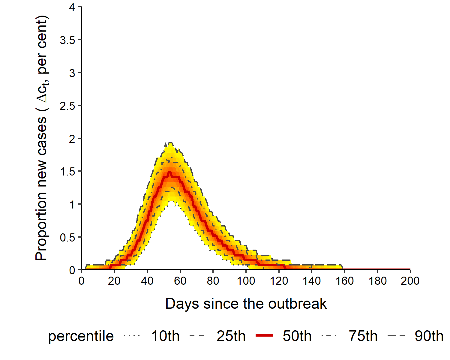
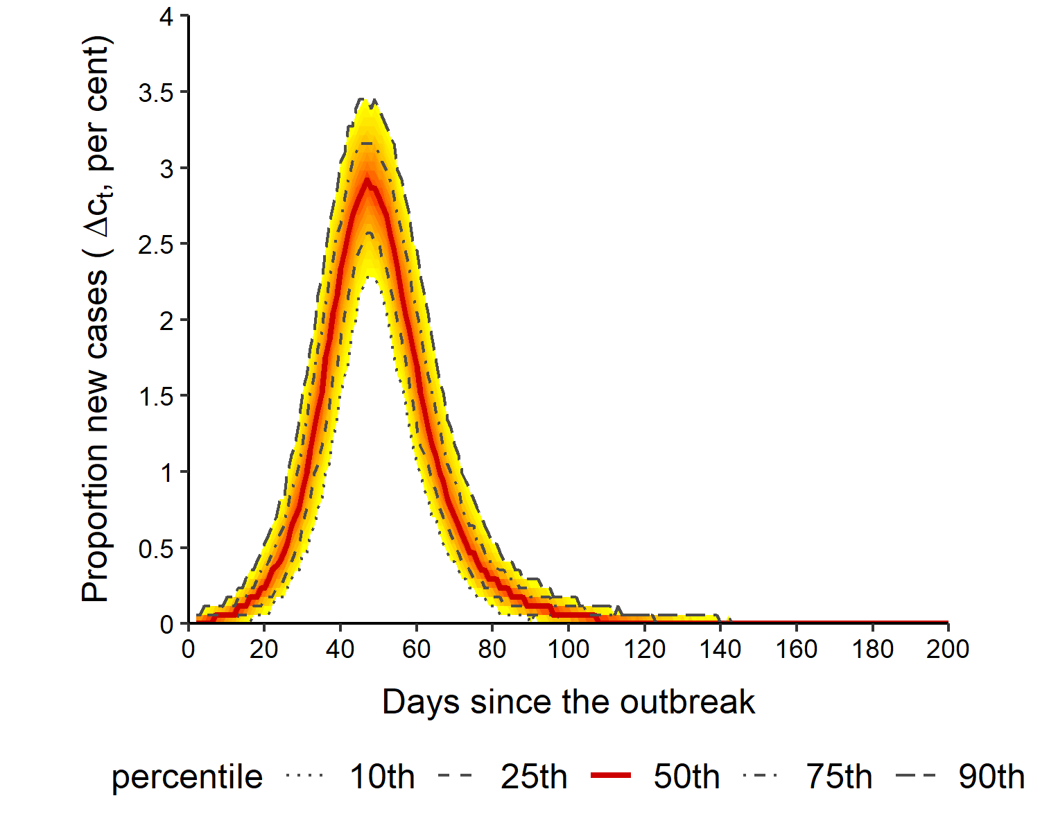
$c_{1}^{\ast}=0.62$		$c_{2}^{\ast}=0.95$
Group 3: [30, 50)		Group 4: [50, 65)
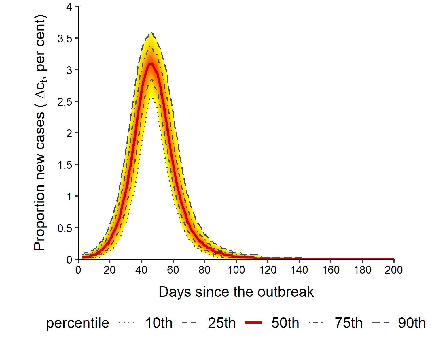
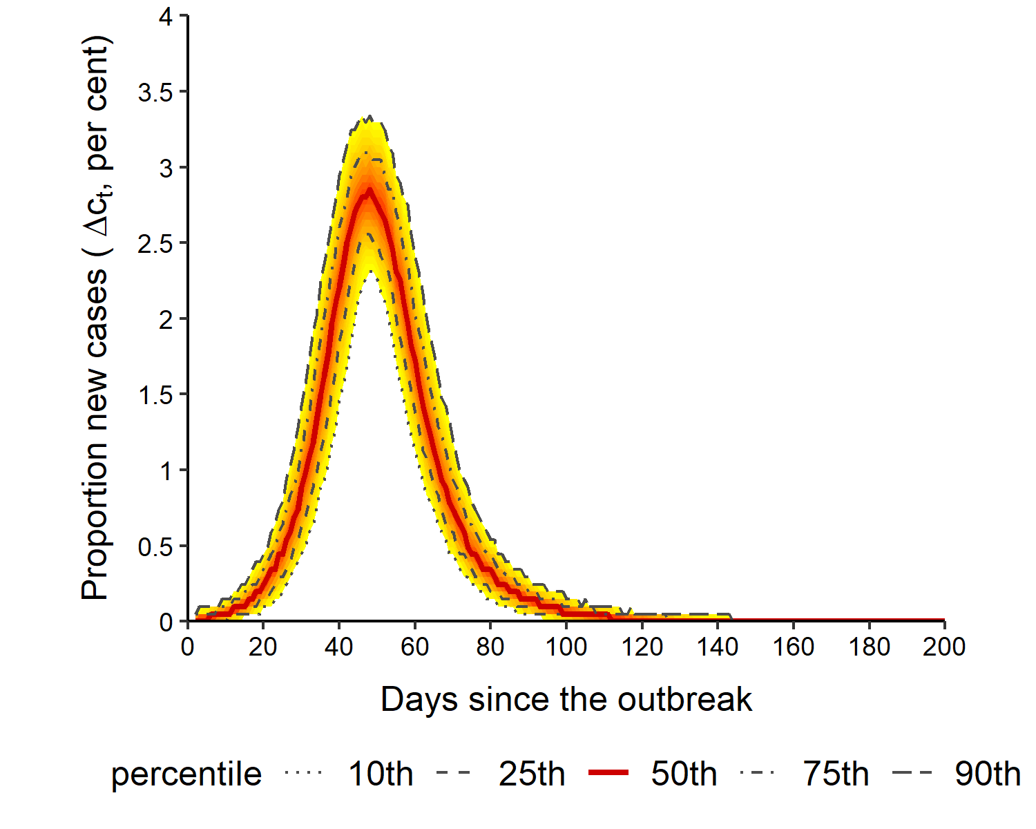
$c_{3}^{\ast}=0.97$		$c_{4}^{\ast}=0.94$
Group 5: 65+		Aggregate
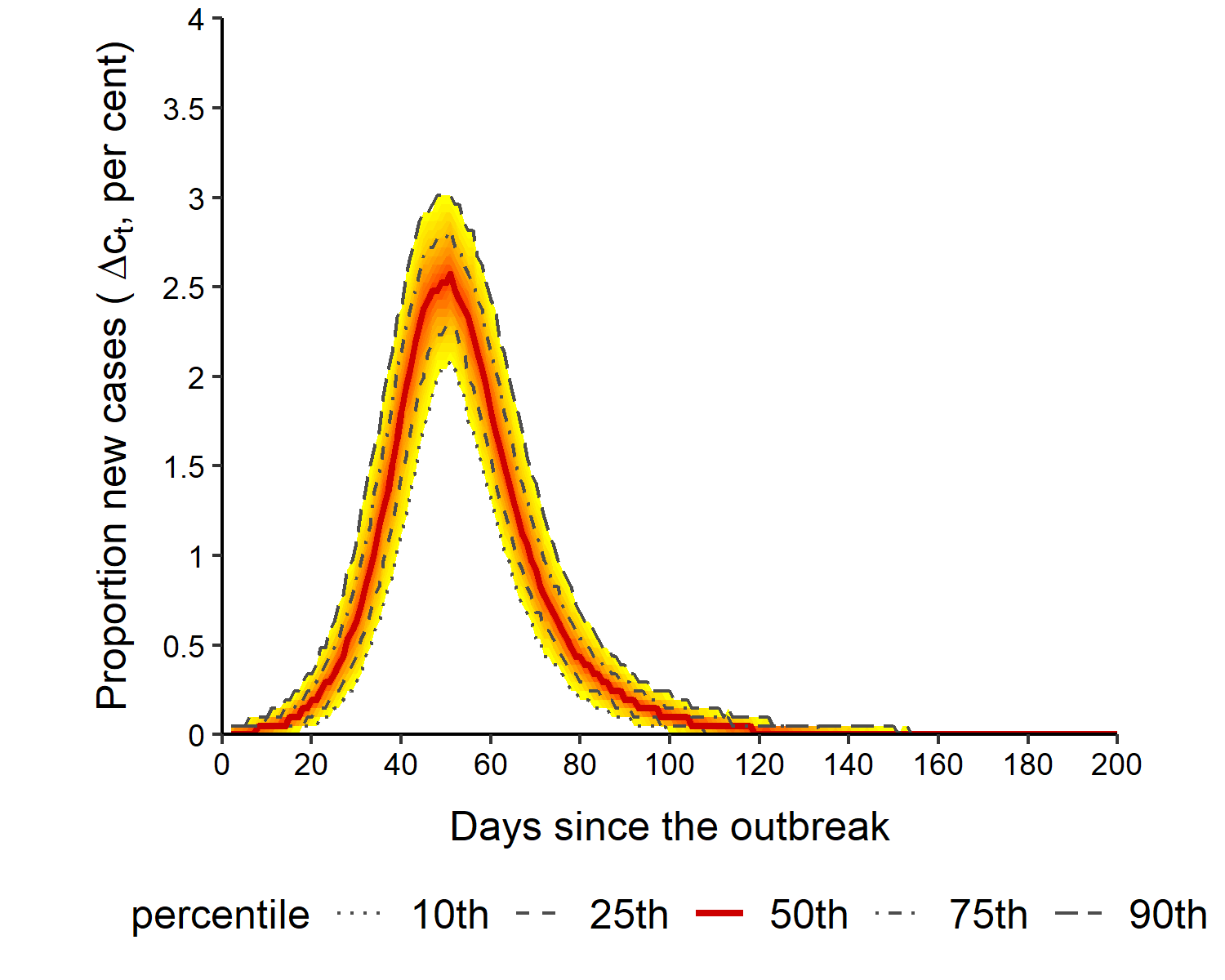
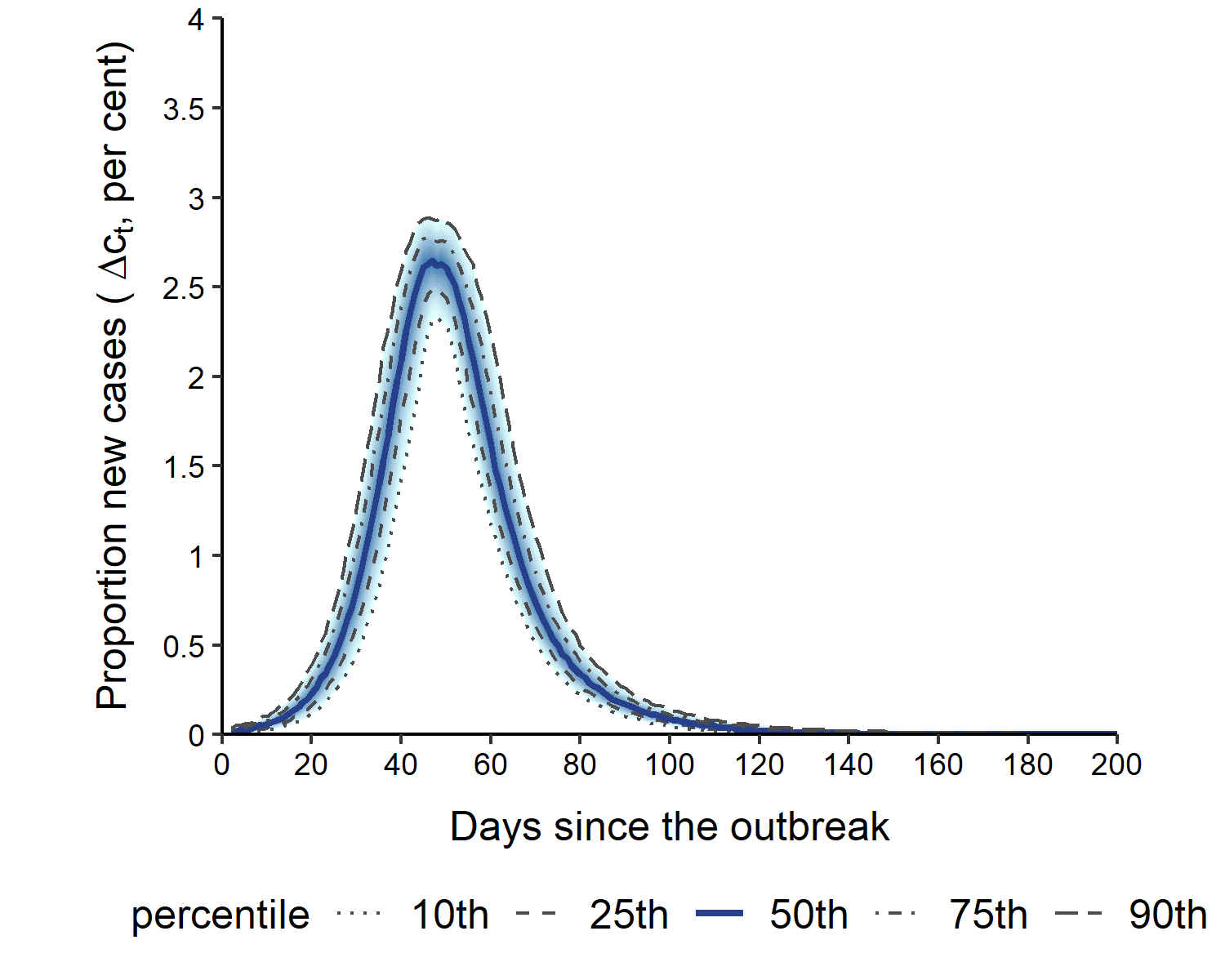
$c_{5}^{\ast}=0.90$		$c^{\ast}=0.90$

Notes: The duration of the epidemic is $T^{\ast}=215$ days. $c_{\ell}^{\ast}=B^{-1}\sum_{b=1}^{B}\max_{t}c_{\ell t}^{(b)}$, for $\ell=1,2,\ldots,L$, and $c^{\ast}=B^{-1}\sum_{b=1}^{B}\max_{t}c_{t}^{(b)}.$ The number of replications is $B=1,000$. Population size is $n=10,000$.

In order to examine whether the number of groups affects the aggregate outcomes, we carry out simulations using a single group model and compare the results with the aggregate outcomes using the multigroup model. When there is only one group, the contact network reduces to the Erdős-Rényi random network (simply referred to as the random network below), where each pair of the nodes (or individuals) are connected at random with a uniform probability $p=k/\left(n-1\right)\approx k/n,$ where $k$ is the mean degree of the network (or the mean number of contacts per individual). We set the average number of contacts to $k=10$ based on the literature on social contacts in the pre-Covid period, and then set the exposure intensity parameter to $\tau=\beta/k=\gamma\mathcal{R}_{0}/k$, where, as before, $\gamma=1/14$ and $\mathcal{R}_{0}=3$. Figure S.2 of the online supplement shows that the simulated aggregate outcomes are very close under the single- and multi-group models. This finding is reasonable because the simulations were performed with the same fixed $\beta=\gamma\mathcal{R}_{0}$. The heterogeneity in $\tau_{\ell}$ and $p_{\ell\ell^{{}^{\prime}}}$ affects the epidemic curves for each group but does not seem to impact the aggregate outcomes. This result suggests that an aggregate analysis may be justified if the primary focus is on the spread of the infection across the population as a whole rather than on particular age/type groups.

Lastly, to investigate whether the results are robust to different network topologies, we considered another widely used contact network—the power law random network, in which a small number of nodes (individuals) may have a relatively high number of links (contacts). Figure S.4 of the online supplement shows that the simulation outcomes obtained by the Erdős-Rényi and the power law networks with the same average number of contacts are very similar.

6 Estimation of transmission rates

The previous section investigates the properties of the model, assuming the transmission rates are given. This section turns to detailing how to estimate the transmission rate using data on infected cases. We first derive the method of moments estimation of the transmission rate when there are no measurement errors and present the finite sample properties of the estimators using Monte Carlo techniques. We then allow for under-reporting of infected cases and propose a recursive joint estimation of the transmission rate and the degree of under-reporting by a simulated method of moments.

6.1 Estimation without measurement errors

Let us first consider the case of a single group, and recall that the moment condition for this case is given by (32), which is replicated here for convenience

$$E\left(\left.\frac{1-c_{t+1}}{1-c_{t}}\right|\text{ }i_{t}\right)=e^{-\beta i_{t}}+O\left(n^{-1}\right).$$ (48)

We can estimate the transmission rate, $\beta$, using (48) by nonlinear least squares (NLS) given time series data on $\left\{c_{t},i_{t}\right\}$. The recovery rate, $\gamma$, can be estimated using the recovery equation, (29), $E\left(r_{t+1}|r_{t},c_{t}\right)=\left(1-\gamma\right)r_{t}+\gamma c_{t}$. Nevertheless, in reality, $r_{t}$ is often not recorded in a timely manner and $\gamma$ is estimated from the hospitalization data. We therefore set $\gamma=1/14$ in our estimation and calibration exercises, and discuss the properties of the moment estimator of $\gamma$ in the online supplement.

In the absence of any interventions (voluntary or mandatory), we have $\beta=\gamma\mathcal{R}_{0}$, where, as before, $\mathcal{R}_{0}$ is the basic reproduction number. It follows that $\mathcal{R}_{0}$ can be estimated by $\mathcal{\hat{R}}_{0}=\hat{\beta}/\gamma$, where $\hat{\beta}$ is the NLS estimate of $\beta$ using (48). Under social interventions, the recovery equation holds (since $\gamma$ is unaffected), but the moment condition for $c_{t+1}$ now depends on the time-varying transmission rate, $\beta_{t}$. For $\gamma$ in the range of $1/14$ to $1/21$, it is reasonable to use two or three weeks rolling windows when estimating $\beta_{t}$. For a window of size $W$, we have

$$\hat{\beta}_{t}\left(W\right)=\text{Argmin}_{\beta}\sum_{\tau=t-W+1}^{t}\left(\frac{1-c_{\tau}}{1-c_{\tau-1}}-e^{-\beta\text{ }i_{\tau-1}}\right)^{2}.$$ (49)

Note that even though the time series $\left\{c_{t},i_{t}\right\}$ over the course of the epidemic are non-stationary, the rolling estimation is based on short-$T$ series ($T=14$ or $21$).

To examine the finite sample performance of $\hat{\beta}_{t}\left(W\right)$, we estimate $\beta$ using the simulated data generated from the single group stochastic SIR model on a random network with mean contact $k=10$ and assuming $1/1000$ of the population is randomly infected on day $1$. The true value of the transmission rate is set to $\beta=3/14$ such that $\mathcal{R}_{0}=\beta/\gamma=3$. We consider population sizes $n=10,000$, $50,000,$ and $100,000$, and set the the number of replications to $B=1,000$. Recall that $T$ is fixed and $n\rightarrow\infty$. To alleviate noise induced by zero and near-zero observations at the start and final stages of the epidemic, the rolling estimation of $\beta$ is carried out over the $4^{th}-15^{th}$ weeks after the outbreak.

Since the value of $\beta$ is quite small, we present the estimation results in terms of $\mathcal{\hat{R}}_{0}\left(W\right)=\hat{\beta}_{t}\left(W\right)/\gamma$. Table 1 summarizes the bias and root mean square error (RMSE) of the 2-weekly rolling estimates of $\mathcal{R}_{0},$ averaged over the four non-overlapping 3-weekly sub-samples, for different population sizes. The bias is computed as $B^{-1}\sum_{b=1}^{B}\left[\mathcal{\hat{R}}_{0}^{\left(b\right)}\left(W\right)-\mathcal{R}_{0}\right]$, and the RMSE is computed by $\sqrt{B^{-1}\sum_{b=1}^{B}\left[\mathcal{\hat{R}}_{0}^{\left(b\right)}\left(W\right)-\mathcal{R}_{0}\right]^{2}}$, where $\mathcal{\hat{R}}_{0}^{\left(b\right)}\left(W\right)=\hat{\beta}_{t}^{(b)}\left(W\right)/\gamma$ and $\hat{\beta}^{(b)}\left(W\right)$ is the estimate of $\beta$ in the $b^{th}$ simulated sample. As can be seen from Table 1, although $\mathcal{\hat{R}}_{0}$ tends to slightly underestimate $\mathcal{R}_{0}$, its bias and RMSE are quite small in all experiments and sub-samples. The RMSE declines as the population size $n$ increases, but $\mathcal{R}_{0}$ can be estimated reasonably well even with $n=10,000$. Comparing the results over different epidemic stages, the RMSE is relatively larger at the early and late stages of the epidemic. This finding is not surprising since it is difficult to obtain precise estimates when $c_{t}$ and $i_{t}$ are near zero. We also considered the 3-weekly rolling estimates, reported in Table S.1 of the online supplement, and as can be seen are very close to the 2-weekly estimates, with slightly better performance in the early and late stages of the epidemic. We will hereafter mainly focus on the 2-weekly rolling estimation.

Table 1: Finite sample properties of the 2-weekly rolling estimates of $\mathcal{R}_{0}$, in the case where it is fixed at ${\mathcal{R}_{0}}=3$

		3-weekly sub-samples
Weeks since the outbreak		$4^{th}-6^{th}$	$7^{th}-9^{th}$	$10^{th}-12^{th}$	$13^{th}-15^{th}$
Population
$n=10,000$	Bias	-0.0108	-0.0038	-0.0006	0.0014
	RMSE	0.0988	0.0563	0.1048	0.2436
$n=50,000$	Bias	-0.0017	-0.0001	-0.0010	-0.0012
	RMSE	0.0405	0.0251	0.0481	0.1070
$n=100,000$	Bias	-0.0002	0.0005	-0.0003	-0.0009
	RMSE	0.0282	0.0172	0.0335	0.0771

Similar moment conditions can also be used to estimate the parameters of the multigroup model. If time series data on $\left\{c_{\ell t},i_{\ell t}\right\}$, for $\ell=1,2,\ldots,L$ ($L$ is finite) are available, we can estimate $\beta_{\ell\ell^{\prime}}$ using the moment conditions (30), namely,

$$E\left(\left.\frac{1-c_{\ell,t+1}}{1-c_{\ell t}}\right|\text{ }\mathbf{i}_{t}\right)=\exp\left(-\sum_{\ell^{\prime}=1}^{L}\beta_{\ell\ell^{\prime}}i_{\ell^{\prime}t}\right)+O\left(n^{-1}\right).$$

Then, as we have discussed in Section 4, $\beta_{\ell\ell^{\prime}}$ is identifiable from (38) for given values of $\gamma$ and $\mathbf{w=(}w_{1},w_{2},\ldots,w_{L})^{\prime}.$

6.2 Estimation allowing for measurement errors

It is widely recognized that in practice $c_{t}$ and $r_{t}$ are under-reported. The magnitude of under-reporting is measured by the multiplication factor (MF) in the literature (see, e.g., Gibbons et al., 2014). It is expected that the MF will decline over time since data quality will improve as more testing is conducted, but, in any case, MF is certainly greater than one. Denoting the multiplication factor by $m_{t},$ and denoting the observed values of $c_{t}$ and $i_{t}$ by $\tilde{c}_{t}$ and $\tilde{\imath}_{t}$, respectively, we have $c_{t}=m_{t}\tilde{c}_{t}$ and $i_{t}=c_{t}-r_{t}=m_{t}\tilde{\imath}_{t}$ (assuming that $r_{t}=R_{t}/n=m_{t}\tilde{r}_{t}$, where $\tilde{R}_{t}$ is the observed value of $R_{t}$). Then the moment condition in terms of the observed values ($\tilde{c}_{t}$ and $\tilde{\imath}_{t}$) can be written as

$$E\left(\left.\frac{1-m_{t+1}\tilde{c}_{t+1}}{1-m_{t}\tilde{c}_{t}}\right|\text{ }\tilde{\imath}_{t},\tilde{c}_{t}\right)=e^{-\beta_{t}m_{t}\tilde{\imath}_{t}}+O\left(n^{-1}\right).$$ (50)

It can be seen from (50) that $m_{t}$ is not identified when $\tilde{c}_{t}$ and $\tilde{\imath}_{t}$ are very small in the early stage of the epidemic. When $\tilde{c}_{t}$ becomes large enough, we can estimate $m_{t}$ by the simulated method of moments based on (50). In practice, $m_{t}$ varies slowly, and it is reasonable to assume $m_{t}=m_{t-1}$ within a short time interval (two or three weeks). Then we have

$$\frac{1-m_{t}\tilde{c}_{t}}{1-m_{t}\tilde{c}_{t-1}}=B^{-1}\sum_{b=1}^{B}e^{-\beta_{t-1}i_{t-1}^{\left(b\right)}}\text{,}$$ (51)

where $i_{t}^{\left(b\right)}$ denotes the simulated value of $i_{t}$ in the $b^{th}$ replication and $B$ is the total number of replications. Solving (51) for $m_{t}$ yields

$$m_{t}=\frac{1-B^{-1}\sum_{b=1}^{B}e^{-\beta_{t}i_{t-1}^{\left(b\right)}}}{\tilde{c}_{t}-\left(B^{-1}\sum_{b=1}^{B}e^{-\beta_{t-1}\imath_{t-1}^{\left(b\right)}}\right)\tilde{c}_{t-1}}.$$ (52)

It is now clear that one can estimate $m_{t}$ by (52) for given values of $\beta_{t}$, and estimate $\beta_{t}$ by (49) if $m_{t}$ is known. Accordingly, we propose a method that estimates $\beta_{t}$ and $m_{t}$ jointly. The algorithm is described in detail in Section S4.1 of the online supplement. We apply the procedure recursively using 2- and 3-weekly rolling windows in the next section to examine how the transmission rates and under-reporting of cases changed over time in a number of countries and evaluate how our model matches the Covid-19 evidence.

7 Matching the model with evidence from a number of European countries

We now assess how our model matches with the recorded cases in six European countries: Austria, France, Germany, Italy, Spain, and the United Kingdom, while taking account of under-reporting of infections. The Covid-19 outbreak in Europe began with Italy in early February 2020, with the recorded number of infections accelerating rapidly from February 21 onward. A rapid rise in infections took place about one week later in Spain, France, and Germany, followed by UK and Austria at the end of February.

To estimate $\beta_{t}$, we need observations on per capita infected and active cases, $c_{t}$ and $i_{t}$. Using the recorded number of infected cases, $\tilde{C}_{t}$, and population data, the per capita cases, $\tilde{c}_{t}$, are readily available, where as before we use the tilde symbol to indicate observed values. Since $\tilde{I}_{t}=\tilde{C}_{t}-\tilde{R}_{t}$, we can obtain $\tilde{I}_{t}$ if the number of removed (the sum of those who recovered and the deceased) cases, $\tilde{R}_{t}$, is available. Unfortunately, the recovery data is either not reported or is subject to severe measurement error/reporting issues in many countries. For all six countries, we therefore estimate the number of removed using the recursion $\tilde{R}_{t}=\left(1-\gamma\right)\tilde{R}_{t-1}+\gamma\tilde{C}_{t-1}$, for $t=2,3,\ldots,T$, where the recovery rate $\gamma$ is set to $1/14,$ and values of $\tilde{R}_{t}$ are generated starting with $\tilde{R}_{1}=\tilde{C}_{1}=0$. We then compute $\tilde{I}_{t}$ by subtracting the estimated $\tilde{R}_{t}$ from the recorded $\tilde{C}_{t}$. That is, in this empirical exercise, we only need data on Covid-19 cases per capita, $\tilde{c}_{t}$. To alleviate the wide fluctuations in the data due to irregular update schedules and reporting/recording delays, we smooth the series by taking the 7-day moving average before they are used in the estimation and calibration.

We adopt the joint estimation approach proposed in the last section to calibrate and evaluate our stochastic network model. The procedure is applied recursively using 2- and 3-weekly rolling windows. Recall that in the early stage of an epidemic, $\tilde{c}_{t}$ is small, and MF is not identified. We choose $\tilde{c}^{0}=0.01$ as the threshold value. When $\tilde{c}_{t}\leq\tilde{c}^{0}$, we use an initial guess of the multiplication factor, MF $=5$, in the estimation of $\beta_{t}$. Since the early Covid data are quite noisy, we start the rolling estimation when the daily new cases exceed one per $100,000$ people and use the estimates below $\mathcal{R}_{0}=3$ in the calibration. Specifically, the simulations begin with $1/1000$ of the population randomly infected on day $1$. To render the calibrations comparable across the countries in our sample, during the first week after the outbreak we set the value of $\beta$ such that $\mathcal{R}_{0}$ equals its first estimate, $\hat{\beta}_{t}/\gamma$, that is less than $3$. Then, from the second week onwards, we set $\beta_{t}$ to the rolling estimates computed from the realized data (with MF $=5$) until $\tilde{c}_{t}$ reaches $\tilde{c}^{0}$ on day $t^{0}$. As shown in Section 5, it makes little difference to the aggregate outcomes whether we carry out the simulations using single- or multi-group models. Since we are interested in comparing the calibrated outcomes with realized cases, we conduct simulations using the single group model with the Erdős-Rényi random network in this exercise. The first estimate of MF is computed as the ratio of the average calibrated cases to realized cases on day $t^{0}$. When $\tilde{c}_{t}>\tilde{c}^{0}$, we perform the joint rolling estimation of $\beta_{t}$ and $m_{t}$ using (S.9) and (S.10). We present the 2-weekly estimation and calibration results in the main paper. The results using the 3-weekly rolling windows are very close and are given in the online supplement. Since the moment condition, (50), used in the joint estimation was derived assuming no vaccination, we end the joint estimation when the recorded share of the population fully vaccinated reaches $10$ percent. The population size in simulations is set to $n=50,000$. To ease the computational burden, the number of replications is set to $B=500$.

Figure 2: Rolling estimates of the effective reproduction numbers ($\mathcal{R}_{et}$) for selected European countries, with start and end dates of the respective lockdowns

Austria		France
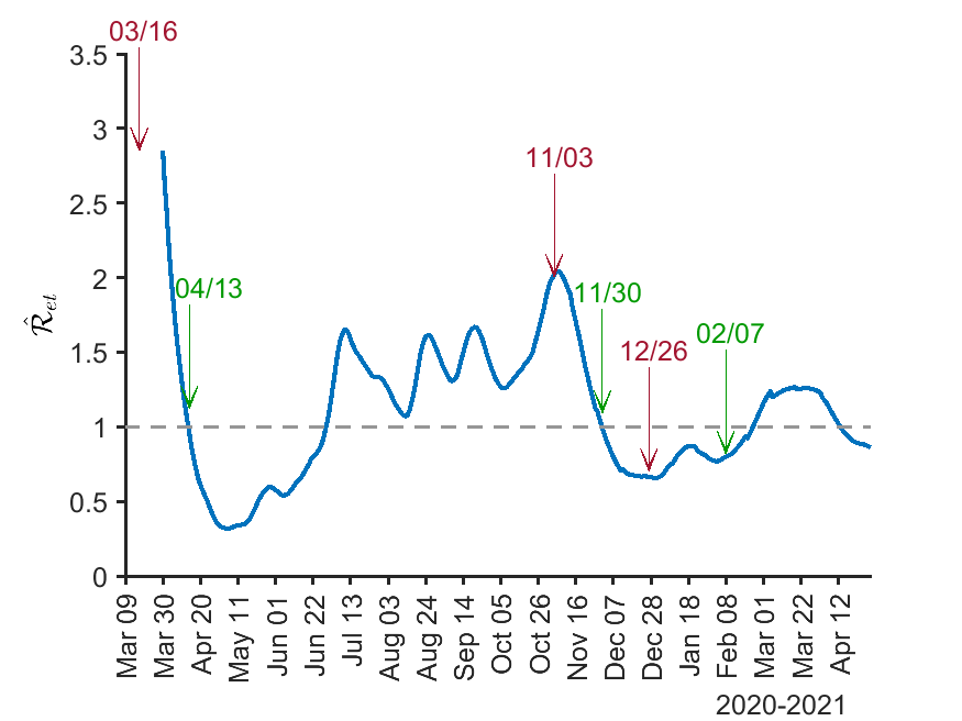
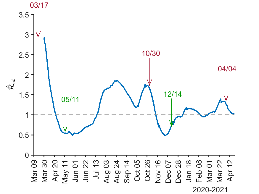
Germany		Italy
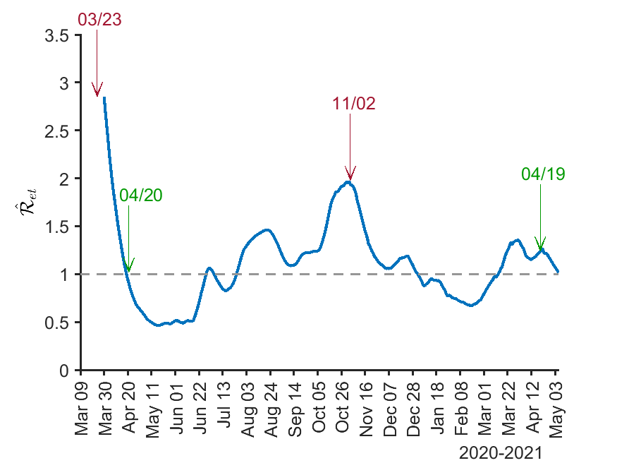
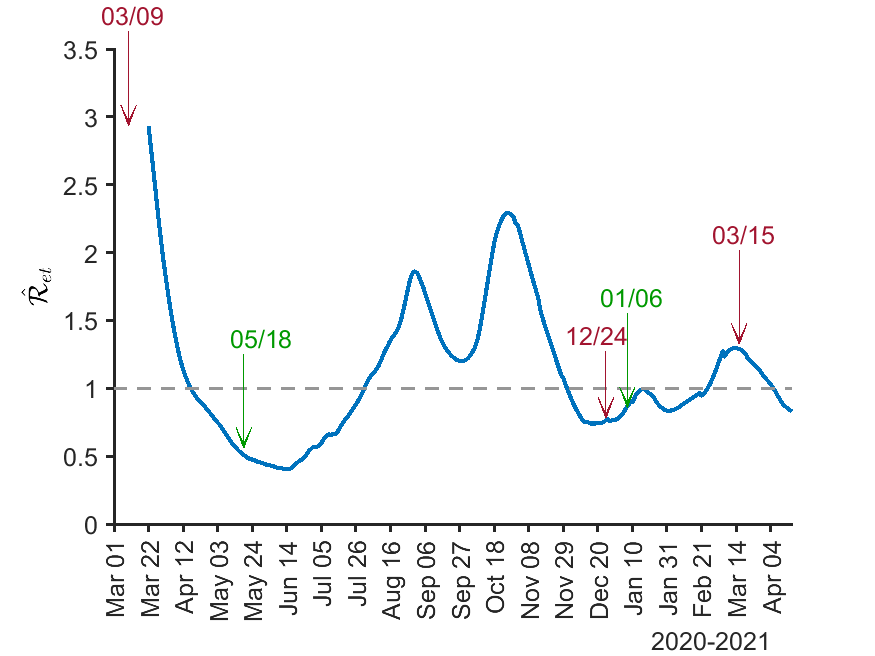
Spain		UK

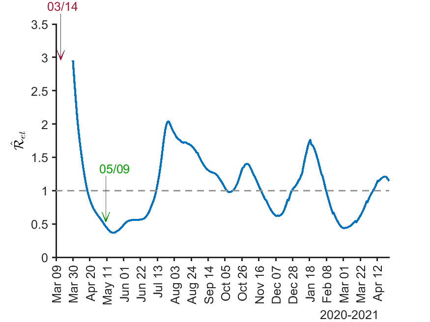
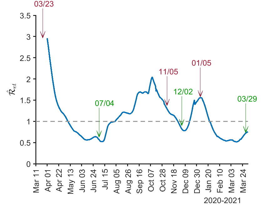
Notes: $\mathcal{\hat{R}}_{et}=\left(1-\hat{m}_{t}\tilde{c}_{t}\right)\hat{\beta}_{t}/\gamma$, where $\tilde{c}_{t}$ is the reported number of infections per capita and $\gamma=1/14$. $W_{\beta}=W_{m}=2$ weeks. The joint estimation starts when $\tilde{c}_{t}>0.01$. The initial guess estimate of the multiplication factor is $5$. The simulation uses the single group model with the random network and population size $n=50,000$. The number of replications is $500$. The number of removed (recoveries + deaths) is estimated recursively using $\tilde{R}_{t}=\left(1-\gamma\right)\tilde{R}_{t-1}+\gamma\tilde{C}_{t-1}$ for all countries, with $\tilde{C}_{1}=\tilde{R}_{1}=0$. Red (green) arrows indicate the start (end) dates of the respective lockdowns.

Figure 2 shows the evolution of $\mathcal{\hat{R}}_{et}$ over the period March 2020–April 2021 for the six countries, where $\mathcal{\hat{R}}_{et}=\left(1-\hat{m}_{t}\tilde{c}_{t}\right)\hat{\beta}_{t}/\gamma$ and $\hat{m}_{t}$ is displayed in Figure 3. It also marks the start and end dates of the respective lockdowns. It should be noted that the epidemic tends to expand (contract) if $\mathcal{\hat{R}}_{et}$ is above (below) unity. Among the six countries, Italy started the first national lockdown on March 9, 2020, followed by Spain, Austria, and France about a week later, and Germany and the UK two weeks later (on March 23, 2020). As can be seen from Figure 2, $\mathcal{\hat{R}}_{et}$ fell below one in mid to late April 2020 in all these countries except for the UK, which took a bit longer before falling below unity in early May. On average, it took $36$ days to bring $\mathcal{\hat{R}}_{et}$ down below one from the start of the lockdown, with Germany being the fastest ($27$ days) and the UK being the slowest ($47$ days). By the end of May 2020, $\mathcal{\hat{R}}_{et}$ were brought down below $0.5$ in all six countries except for the UK, where the lowest value of $\mathcal{\hat{R}}_{et}$ occurred in early July. As lockdowns eased, not surprisingly, the transmission rates started to rise. This new surge in estimates of $\mathcal{R}_{et}$ led some of the countries to announce their second lockdowns in early November 2020. The estimates of $\mathcal{R}_{et}$ fell below one again in December 2020, but the second trough in $\mathcal{\hat{R}}_{et}$ is higher than the first in all countries except France. As the pandemic progressed, $\mathcal{\hat{R}}_{et}$ displayed different patterns (timing and magnitudes of peaks and troughs) across the six countries due to different containment measures. By late April 2021 (the end of our sample), $\mathcal{\hat{R}}_{et}$ is estimated to be close to one in all these countries, but they appear to be rising in Spain and the UK and falling in the other countries.

Figure 3: Rolling estimates of the multiplication factor for selected European countries

Austria		France
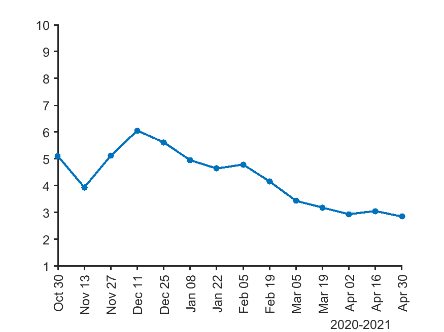
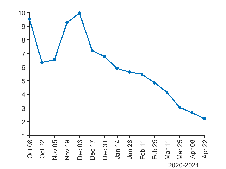
Germany		Italy
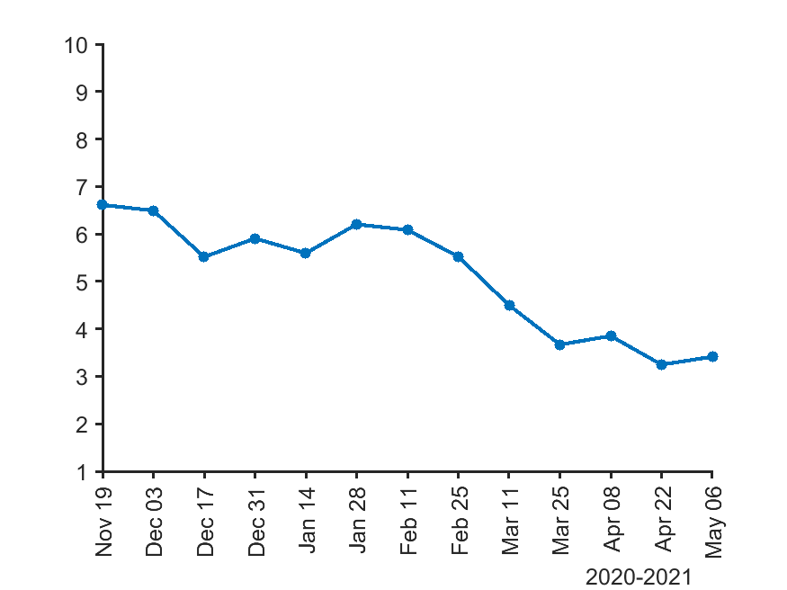
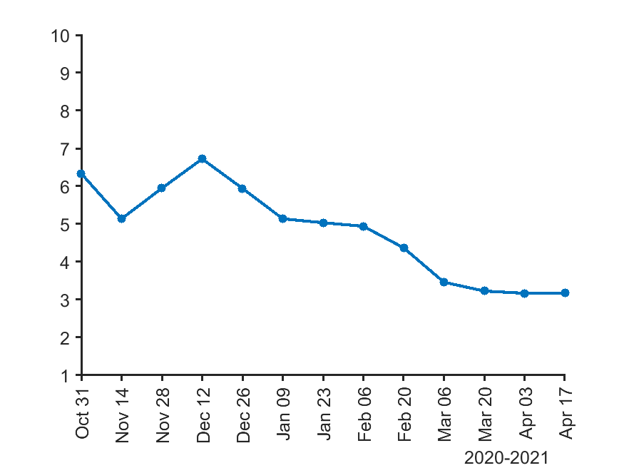
Spain		UK

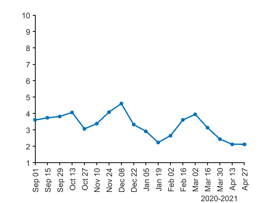
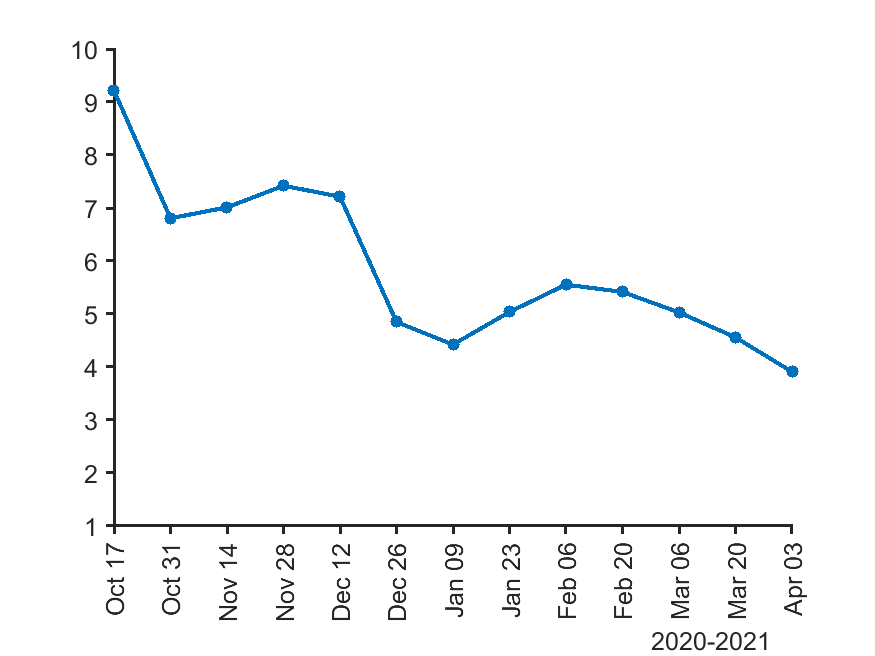
Notes: See the notes to Figure 2.

Figure 3 plots the estimated MF for the six countries. The results offer evidence of substantial under-reporting in the pandemic’s early stages, with the magnitude of under-reporting falling over time in all these countries. Closer inspection of the figure shows that the number of cases in Austria, Germany, and Italy in late October-mid November 2020 was underestimated by $5$–$6$ times, which declined to $2$–$3$ times in late April 2021. About a quarter of actual infections were recorded in Spain in September 2020, compared to about a half being detected in late April 2021. France and the UK have a greater level of under-reporting in the early stages—the number of cases was underestimated by as much as a factor of $9$–$10$, which fell to $2$–$4$ during the study period. Overall, the magnitude of these estimated MF seems reasonable and comparable to the estimates obtained by other approaches in the literature.

Figure 4: Realized and calibrated number of new cases of Covid-19 for selected European countries

Austria		France
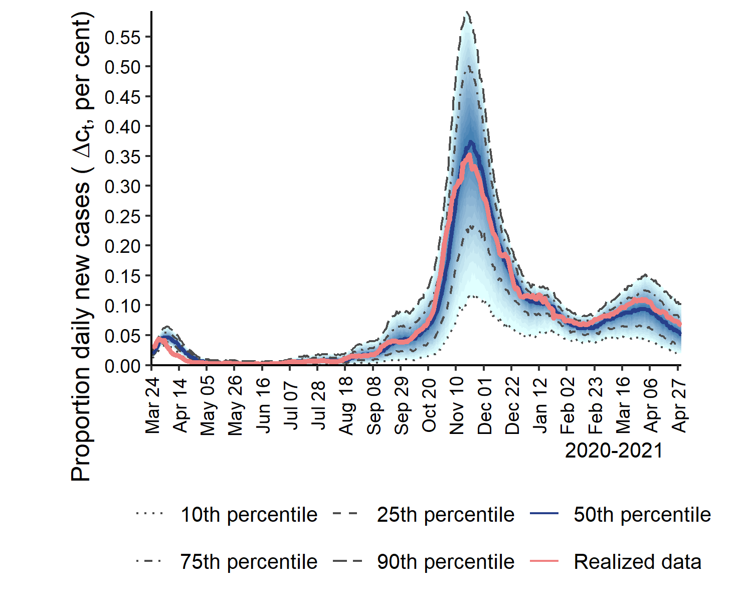
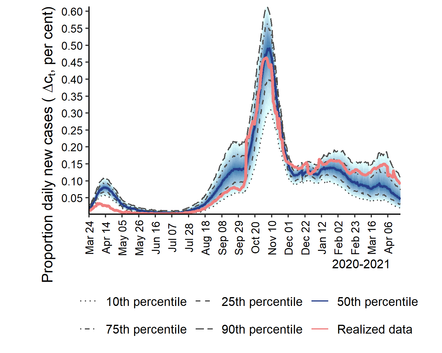
Germany		Italy
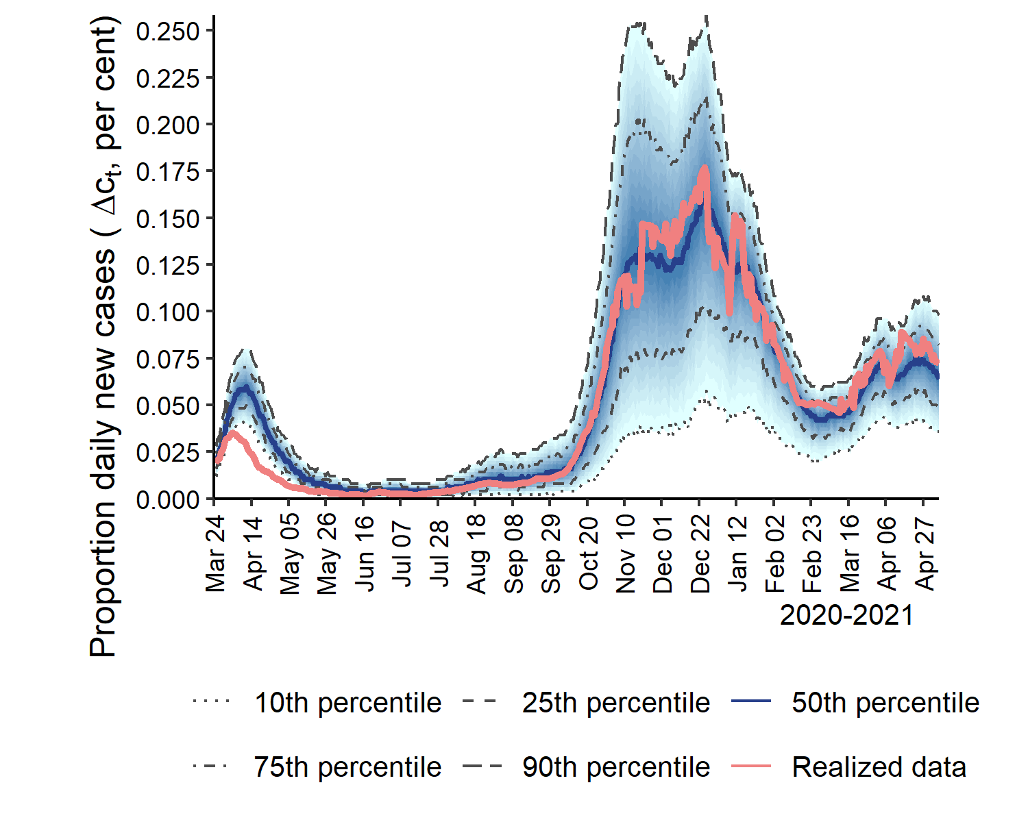
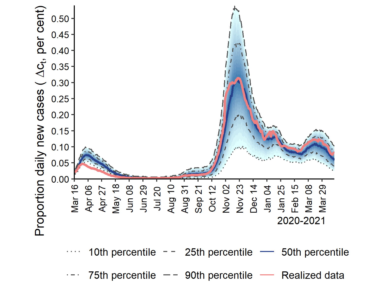
Spain		UK

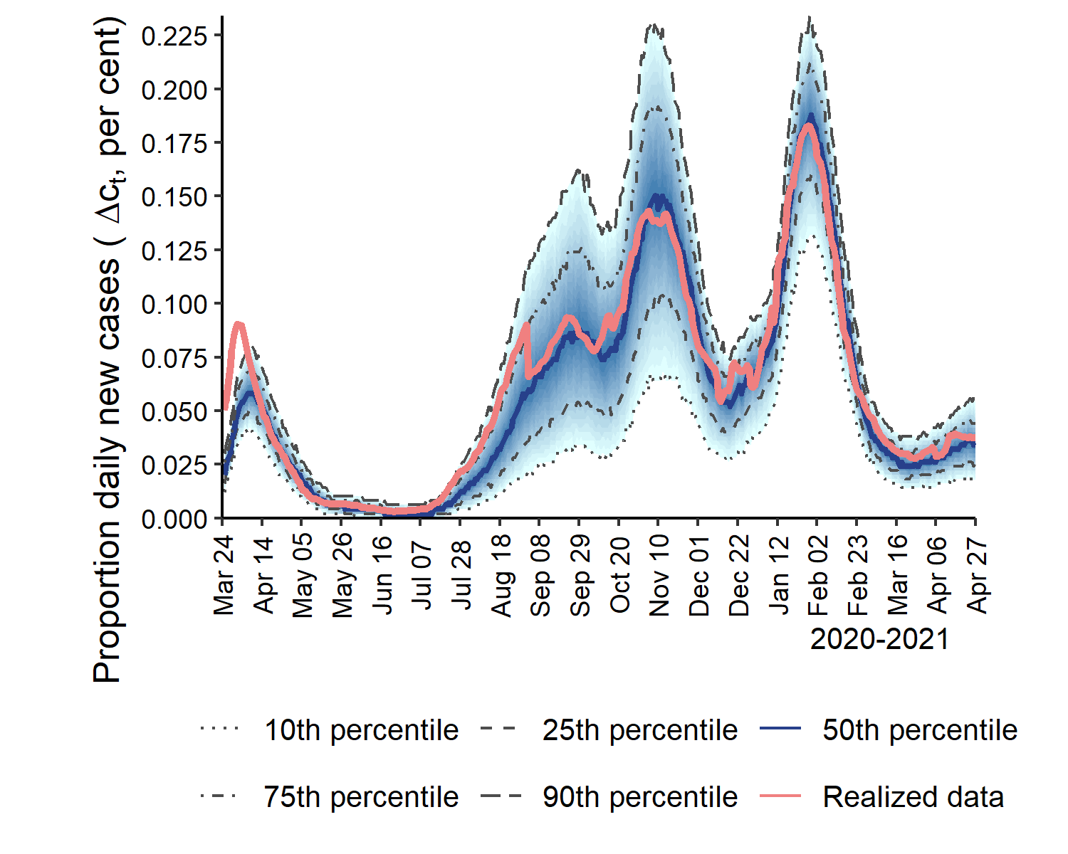
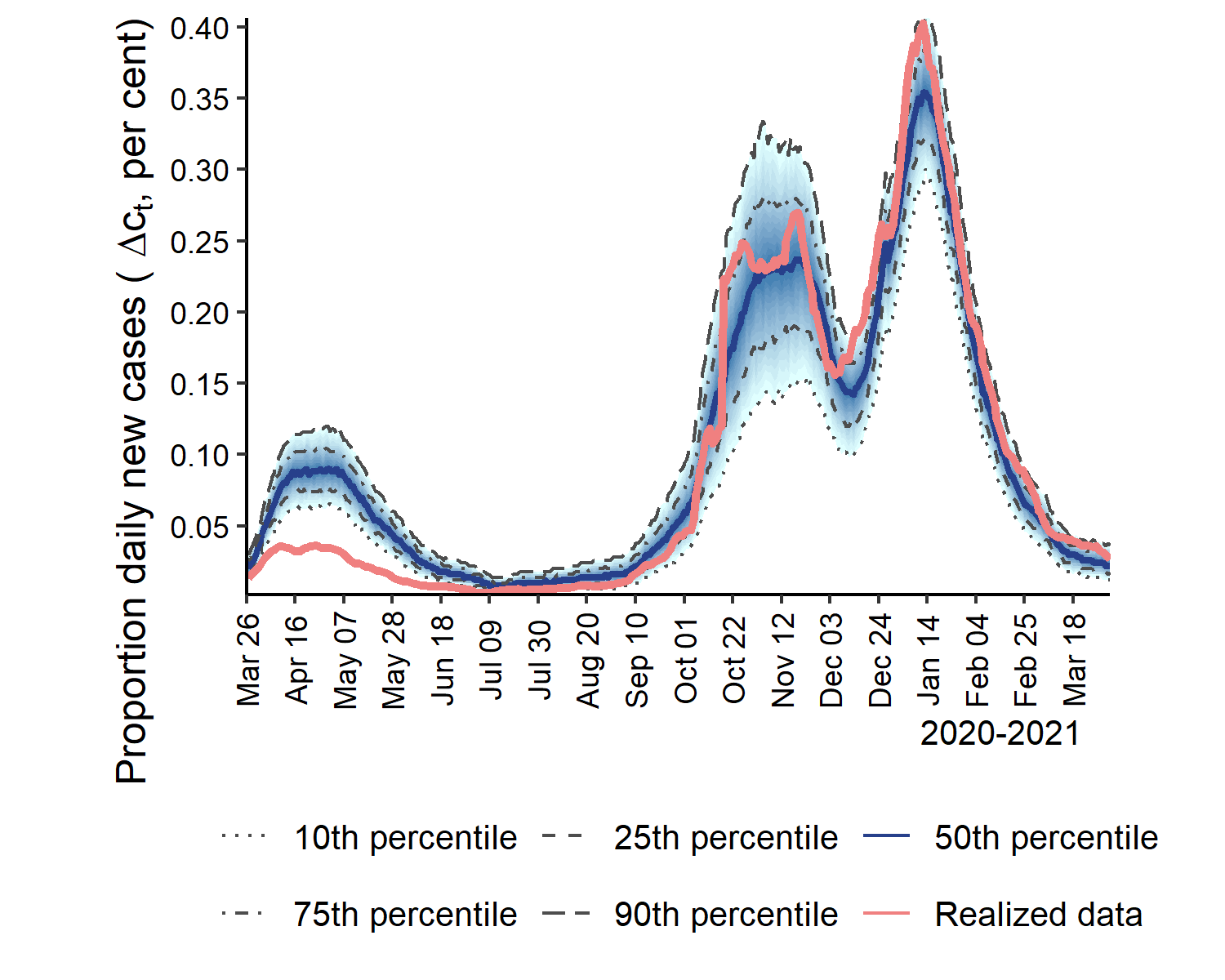
Notes: Realized series (7-day moving average) multiplied by the estimated multiplication factor is displayed in red. See also the notes to Figure 2.

Figure 4 presents the calibrated new cases and the 7-day moving average of the reported new cases multiplied by the estimated MF. The fan charts depict the $10^{th}$ through the $90^{th}$ percentiles of the calibrated data. It can be seen that once we have taken account of under-reporting, the calibrated cases match with the recorded cases fairly well. It is noteworthy that our model is able to catch the multiple waves of Covid-19 cases over the course of the epidemic. Lastly, it is interesting to see how the total cases per capita compare across the six countries, with and without adjustments for under-reporting. Figure S.11 of the online supplement displays the reported total cases and the case numbers after adjusting for under-reporting using the MF estimates. The results show that the number of total cases could have been underestimated three to five times in these countries as of early August 2021. These comparisons clearly show the importance of adjusting the number of infected cases due to under-reporting, which can be reasonably estimated using our joint estimation procedure.

8 Counterfactual exercises

Having shown that the outcomes of the calibrated model closely match the evidence, we now demonstrate how the model can be used for two counterfactual analyses of interest. First, we investigate the impact of social distancing and vaccination on the evolution of the epidemic. To simplify the exposition, we consider an epidemic with two waves and investigate if the second wave can be avoided by vaccination. Second, we consider counterfactual outcomes that could have resulted from different timing of the early interventions in Germany and the UK.

8.1 Social distancing and vaccination

In order to understand the impact of non-pharmaceutical interventions and vaccination on controlling the epidemic, we perform counterfactual analyses using the multigroup model with the five age groups introduced in Section 5. The different age groups in the model also allow us to consider the implications of prioritizing the Covid-19 vaccine by age.

In reality, the transmission rate varies over time due to both voluntary and mandatory social distancing as well as other mitigation measures such as vaccination. Here we use social distancing to refer broadly to all types of non-pharmaceutical interventions (including lockdown measures). We assume that, in the absence of a vaccination program, the (scaled) transmission rate, $\beta_{t}/\gamma$, equals $3$ in the first two weeks after the epidemic outbreak, falls to $0.9$ linearly over the next three weeks, and remains at $0.9$ for eight weeks. When social distancing is relaxed, the transmission rate increases to $1.5$ linearly over the next three weeks and remains at $1.5$ thereafter. Note that the effective reproduction number, $\mathcal{R}_{t}$, could still fall below unity due to herding. Also note that $\beta_{t}=\sum_{\ell=1}^{L}w_{\ell}\beta_{\ell t}$, where $\beta_{\ell t}=\sum_{\ell^{\prime}=1}^{L}\tau_{\ell t}k_{\ell\ell^{\prime},t}$. We assume that $\beta_{\ell t}$ has the same rate of change as $\beta_{t}$, for all $\ell$.

To model vaccination, we assume, for simplicity, that a single-dose shot vaccine with efficacy of $\epsilon_{v}$ becomes available when $i_{t}=i^{0}$. The vaccine takes full effect immediately, and its immune protection does not wane over time. The effectiveness of vaccination can be measured by the parameter $\mu_{i\ell}$, which is the mean of the infection threshold variable, $\xi_{it}$, defined in (13). We assume that $\mu_{i\ell}$ takes the value $\mu^{0}$ if individual $(i,\ell)$ is not vaccinated and takes the value $\mu^{1}$ after vaccination. In the case of a single group, the probability of an individual getting infected when the proportion of active cases is $i^{0}$, for any given value of $\mu_{i}$, is

$$E\left(x_{i,t+1}\left|x_{it}=0,\mu_{i},i_{t}=i^{0}\right.\right)=1-\left(1-p+pe^{-\frac{\tau}{\mu_{i}}}\right)^{ni^{0}},$$ (53)

which declines with $\mu_{i}$. By definition, the vaccine efficacy should equal the percentage reduction in the probability of infection. Then the value of $\mu_{i}$ associated with efficacy $\epsilon_{v}$ is given by

$$E\left(x_{i,t+1}\left|x_{it}=0,\mu_{i}=\mu^{1},i_{t}=i^{0}\right.\right)-E\left(x_{i,t+1}\left|x_{it}=0,\mu_{i}=\mu^{0},i_{t}=i^{0}\right.\right)$$ (54)

$$=-\epsilon_{v}E\left(x_{i,t+1}\left|x_{it}=0,\mu_{i}=\mu^{0},i_{t}=i^{0}\right.\right)$$

Using the result in (21), we have

$$1-\left(1-p+pe^{-\frac{\tau}{\mu_{i}}}\right)^{ni^{0}}\approx 1-\exp\left(-\frac{\tau ki^{0}}{\mu_{i}}\right)\approx\frac{\tau ki^{0}}{\mu_{i}}.$$ (55)

Combining (53), (54), and (55), we obtain $\tau ki^{0}/\mu^{1}\approx\left(1-\epsilon_{v}\right)\tau ki^{0}/\mu^{0}$, which simplifies to

$$\mu^{1}/\mu^{0}\approx 1/(1-\epsilon_{v}).$$ (56)

This result also holds in the multigroup model. Intuitively, (56) states that an individual becomes $1/\left(1-\epsilon_{v}\right)$ times more immune relative to his/her level of immunity after vaccination.

In simulations, an individual’s degree of resilience, $\xi_{it}$, are i.i.d. draws from an exponential distribution with mean $\mu^{0}$ $(\mu^{1})$ before (after) vaccination. Without loss of generality, we normalize $\mu^{0}=1.$ The Pfizer-BioNTech and Moderna vaccines have been shown to have $95\%$ and $94.1\%$ efficacy rates in preventing symptomatic laboratory-confirmed Covid-19 infection, respectively (Oliver et al., 2020, 2021). Accordingly, using (56) we have $\mu^{1}=20$ for $\epsilon_{v}=0.95$, namely Pfizer and Moderna vaccines increase the level of immunity by a factor of $20$.

We suppose that $75$ percent of the population is vaccinated over $12$ weeks, with an equal number of people vaccinated each day. We consider two vaccination schemes—random vaccination and vaccination in decreasing age order. Under the former, people are randomly selected without replacement for vaccination irrespective of their age. In the latter, older people are vaccinated first. Individuals within an age group are randomly selected for vaccination on each day when their group is eligible. After all people in the oldest group have been vaccinated, the second-oldest group becomes eligible. This process continues until $75$ percent of the population is vaccinated. In both schemes, we assume that vaccination eligibility does not depend on whether an individual is susceptible, infected, or recovered.

Let us first consider the random vaccination scheme. Figure 5 compares the aggregate outcomes when there are (a) no containment measures, (b) social distancing only, (c) vaccination only, and (d) combined social distancing and vaccination. Specifically, the transmission rate, $\beta_{t}/\gamma$, is fixed at $3$ in the absence of social distancing (i.e., in cases (a) and (c)). In case (c), the vaccination starts from the $4^{th}$ week after the outbreak. In case (d), the vaccination starts during the last month of social distancing (i.e., the $10^{th}$ week after the outbreak). In cases (c) and (d), $75$ percent of the population is randomly vaccinated over $12$ weeks, and the vaccine efficacy is set at $\epsilon_{v}=0.95$.

Figure 5: Simulated number of new cases when there are (a) no containment measures, (b) social distancing only, (c) vaccination only, and (d) combined social distancing and vaccination

(a) No containment		(b) Social distancing only
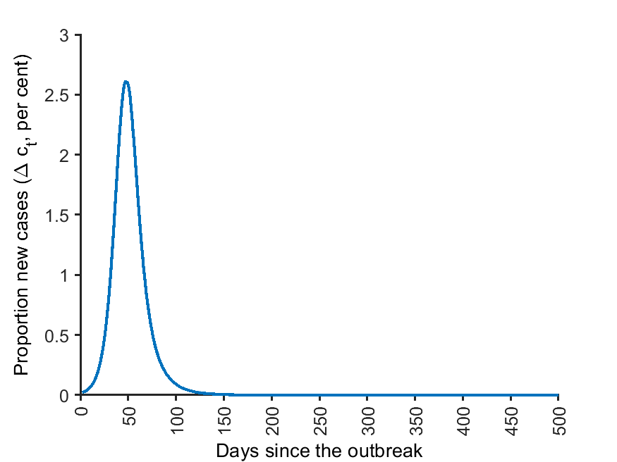
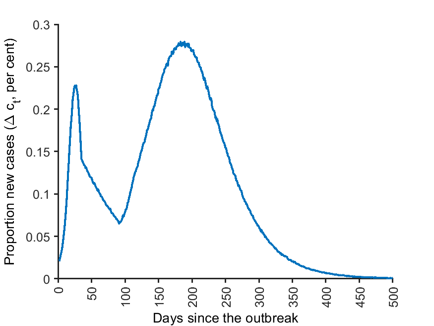
$c^{\ast}=0.90$, $T^{\ast}=215$ days		$c^{\ast}=0.50$, $T^{\ast}=486$ days
(c) Vaccination only		(d) Social distancing and vaccination
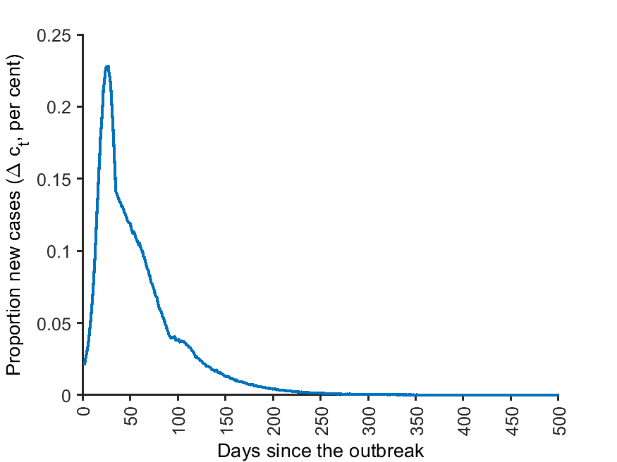
$c^{\ast}=0.59$, $T^{\ast}=201$ days		$c^{\ast}=0.12$, $T^{\ast}=215$ days

Notes: The average number of new cases over $1,000$ replications is displayed. The simulations use the multigroup model with the five age groups as described in Section 5. Population size is $n=10,000$. Under social distancing, the transmission rate, $\beta_{t}/\gamma$, equals $3$ in the first two weeks after the outbreak, falls to $0.9$ linearly over the next three weeks, and remains at $0.9$ for eight weeks. When social distancing is relaxed, the transmission rate increases to $1.5$ linearly over the next three weeks and remains at $1.5$ afterward. In the absence of social distancing (i.e., in cases (a) and (c)), the transmission rate, $\beta_{t}/\gamma$, is fixed at $3$. In case (c), the vaccination starts from the $4^{th}$ week after the outbreak. In case (d), the vaccination starts during the last month of social distancing (i.e., the $10^{th}$ week after the outbreak). In cases (c) and (d), $75$ percent of the population is randomly vaccinated over $12$ weeks, and the vaccine efficacy is $\epsilon_{v}=0.95$. $c^{\ast}$ denotes the maximum proportion of infected and is computed as $B^{-1}\sum_{b=1}^{B}\max_{t}c_{t}^{(b)},$ with $B=1,000$ replications. $T^{\ast}$ is the duration of the epidemic.

The results show that social distancing can quickly bring down the daily case rate and thus reduce the demands on the healthcare system. However, as social distancing restrictions are relaxed, a second wave is expected to emerge. The second wave may have a higher peak than the first wave if the transmission rates rise too fast due to increasing contact rates or the exposure intensity. Comparing graphs (a) and (b) reveal that social distancing alone can reduce the maximum proportion of cases from $90$ percent in an uncontrolled epidemic to $50$ percent. Nonetheless, the duration of the epidemic could more than double, and an enduring epidemic may entail high social and economic costs. If vaccination is the only containment tool, it must be implemented soon enough to curb the spread of the disease, especially for a highly contagious disease with $\mathcal{R}_{0}$ about $3$ (or even higher as evidenced by the new variants). Graph (c) shows that even if (in a very unlikely scenario) a highly effective vaccine becomes available during the $4^{th}$ week after the outbreak, $59$ percent of the population could end up getting infected. In reality, developing a new vaccine takes considerable time. Therefore, vaccination is not a substitute for non-pharmaceutical interventions, which are necessary to slow the spread of the disease, allowing more time for vaccine development. Vaccination can effectively prevent the second wave if it is rolled out during the last month of social distancing, as shown in Graph (d). Under the assumption that $75$ percent of the population end up getting vaccinated with efficacy of $\epsilon_{v}=0.95$, the maximum proportion of infected could reduce to $12$ percent, and the number of highest daily new infections could be more than $10$ and $7$ times lower than that in cases (a) and (c), respectively. We also examined the implications of different vaccination coverages, start times, speeds of delivery, and vaccine efficacies. The results are summarized in Section S7.1 of the online supplement, where we provide counterfactual outcomes assuming (i) 50 percent versus 75 percent vaccination coverage, (ii) vaccination starts at the end of social distancing versus during the last month of social distancing, (iii) 75 percent of the population getting vaccinated over 8 versus 12 weeks, and (iv) $\epsilon_{v}=0.95$ versus $0.66$.

Figure 6: Simulated average number of group-specific and aggregate new cases using the multigroup model with social distancing, assuming random vaccination or vaccination in decreasing age order

Group 1: [0, 15)		Group 2: [15, 30)
Random: $c_{1}^{\ast}=0.04$		Random: $c_{2}^{\ast}=0.13$
By age:  $\ c_{1}^{\ast}=0.05$		By age:  $\ c_{2}^{\ast}=0.17$
Group 3: [30, 50)		Group 4: [50, 65)
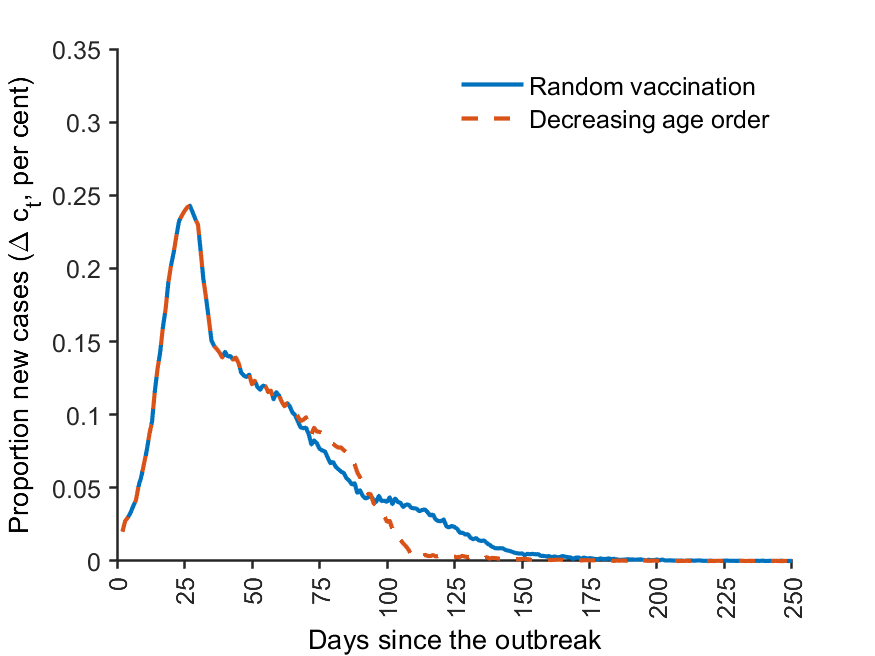
Random: $c_{3}^{\ast}=0.15$		Random: $c_{4}^{\ast}=0.12$
By age:  $\ c_{3}^{\ast}=0.17$		By age:  $\ c_{4}^{\ast}=0.12$
Group 5: 65+		Aggregate
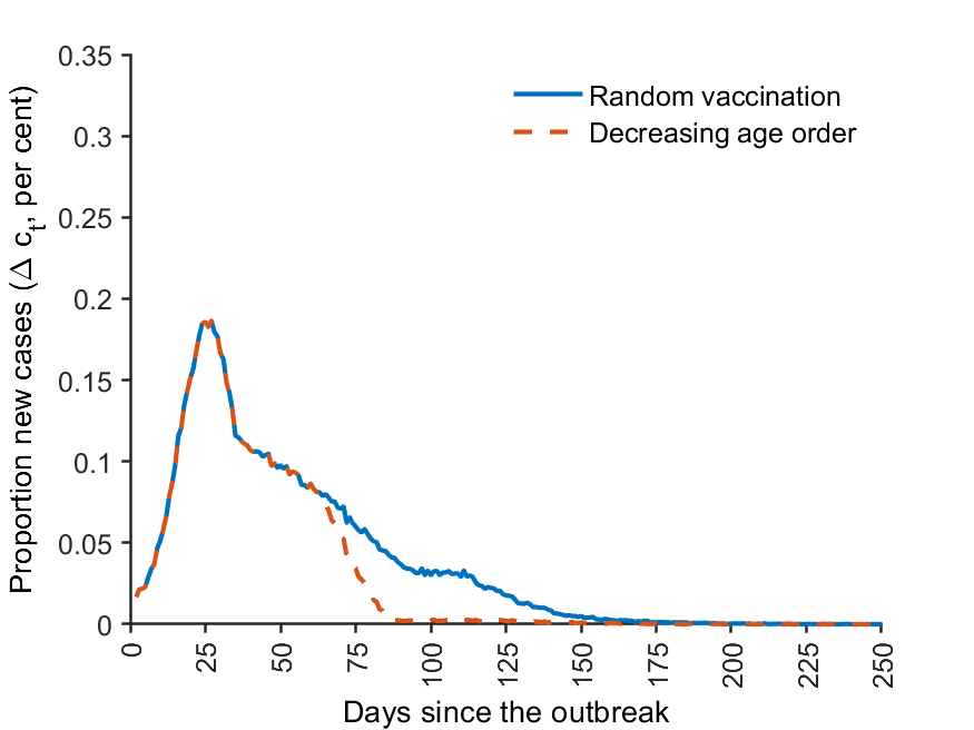
Random: $c_{5}^{\ast}=0.10$		Random: $c^{\ast}=0.12$
By age:  $\ c_{5}^{\ast}=0.08$		By age:  $\ c^{\ast}=0.13$

Notes: The average number of new cases over $B=1,000$ replications is displayed. Population size is $n=10,000$. The social distancing policy is the same as that considered in Figure 5. The vaccination starts during the last month of social distancing (i.e., the $10^{th}$ week after the outbreak). $75$ percent of the population is vaccinated over $12$ weeks. The vaccine efficacy is $\epsilon_{v}=0.95.$ The duration of the epidemic is $T^{\ast}=215$ days under random vaccination and $T^{\ast}=233$ days under vaccination by decreasing age order. $c_{\ell}^{\ast}=B^{-1}\sum_{b=1}^{B}\max_{t}c_{\ell t}^{(b)},$for $\ell=1,2,\ldots,5,$ and $c^{\ast}=B^{-1}\sum_{b=1}^{B}\max_{t}c_{t}^{(b)}$.

Figure 6 compares the simulation outcomes under random vaccination and vaccination in decreasing age order for each age group and the entire population, assuming the same social distancing policy as described above. In this experiment, the vaccination starts during the last month of social distancing. $75$ percent of the population is vaccinated over $12$ weeks, and the vaccine efficacy is $\epsilon_{v}=0.95$. The results show that the maximum proportion of infected in the oldest group is reduced by $2$ percentage points if the old gets vaccinated first, compared to random vaccination. Not surprisingly, the cost of protecting the elderly is reflected in the higher infection rates in the younger age groups, increasing the maximum cases by $1$, $4$, and $2$ percentage points for age groups 1 to 3, respectively. The vaccine effectively curbs the spread of the disease and prevents the second surge of cases in the two senior groups. A comparison of the aggregate outcomes reveals that prioritizing the old results in a higher level of overall infections and a longer duration of the epidemic, owning to higher contact rates of the younger population. Of course, how to prioritize vaccines is a complex decision requiring further information on the rates of hospitalization and death in each age group. It also requires evaluating the social and economic costs of high infection rates and lockdown measures among young people.

8.2 Counterfactual outcomes of early interventions in UK and Germany

We now turn to different counterfactual outcomes that could have resulted from different timing of the first lockdowns in Germany and the UK, focusing on the first wave of Covid-19 that leveled off at the end of June 2020 in both countries. In particular, we investigate the quantitative effect of bringing forward the lockdown in the UK on the number of infected cases, as compared to the effect of delaying the lockdown in Germany. To this end, we shift the estimated $\beta_{t}$ values backward or forward for one or two weeks. As shown in Figure 7, if the German lockdown had been delayed by one week, the maximum proportion of infected cases would have increased from $2.2$ to $5.0$ percent, and the maximum proportion of active cases would have risen from $0.6$ to $1.5$ percent. In contrast, if the UK lockdown had been brought forward by one week, the model predicts that the maximum proportion of infected cases would have reduced from $5.3$ to $2.3$ percent, and the maximum number of active cases would have reduced from $1.2$ to $0.5$ percent. These results suggest that the UK could have achieved a similarly low level of infected cases per capita as Germany if it had implemented social distancing sooner. The maximum proportion of infected (active cases) is estimated to rise further to $10.8$ ($3.2$) percent if the German lockdown was delayed by two weeks, and the maximum proportion of infected (active cases) is estimated to decrease further to $1.1$ ($0.3$) percent if the UK lockdown was brought forward by two weeks. In summary, this counterfactual exercise shows that it is critical to take measures to lower the effective reproduction number as early as possible if a policymaker aims to control the number of infected and active cases.

Figure 7: Counterfactual number of infected and active cases for Germany and UK under different lockdown scenarios

What if the German lockdown was delayed one week?
Infected cases	Active cases	$\mathcal{\hat{R}}_{et}$
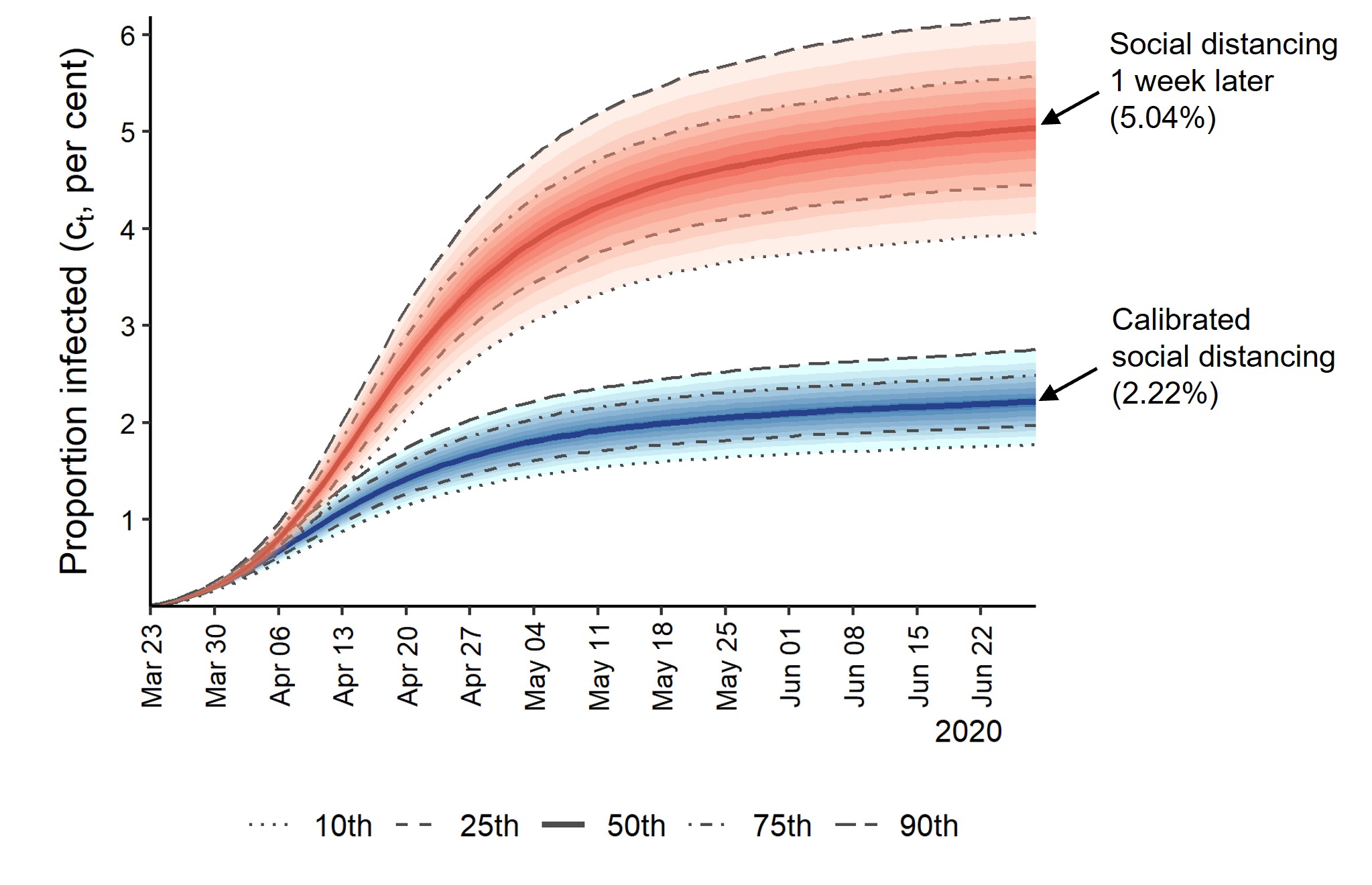
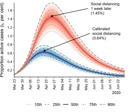
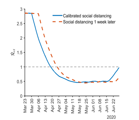
What if the UK lockdown was brought forward one week?
Infected cases	Active cases	$\mathcal{\hat{R}}_{et}$

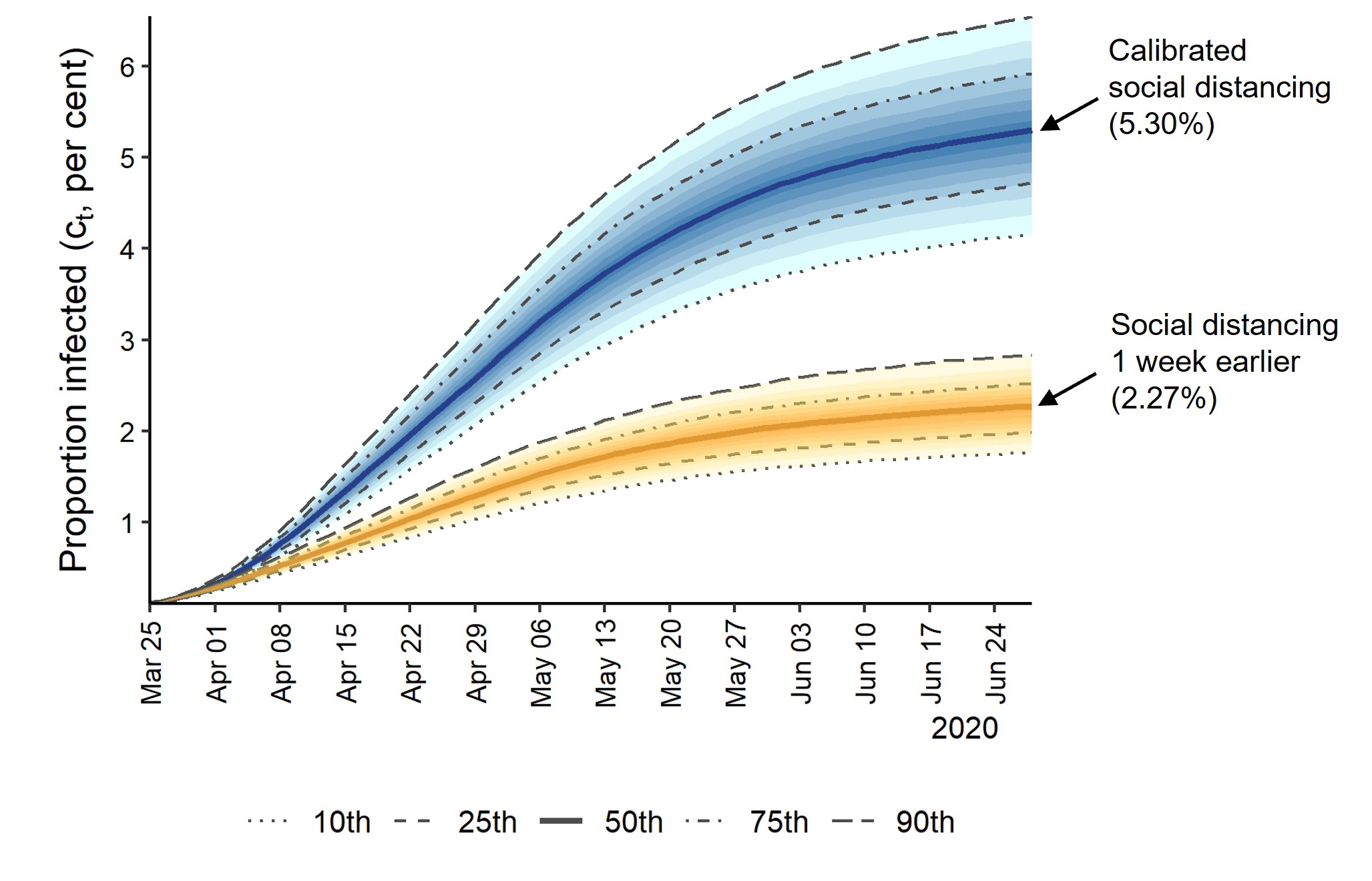
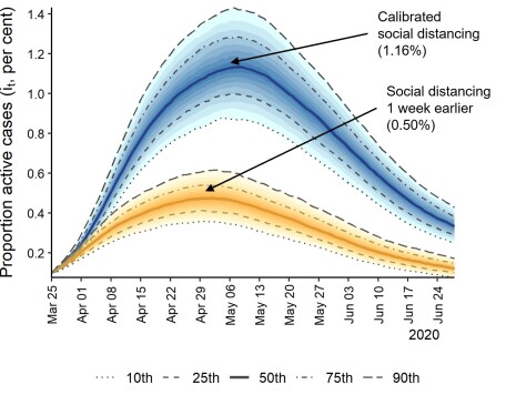
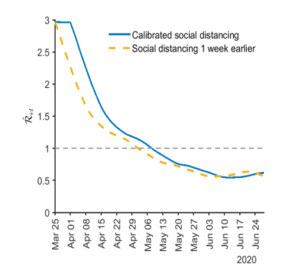
Notes: The simulation uses the single group model with the Erdős-Rényi random network and begins with $1/1000$ of the population randomly infected on day $1$. The population size used in the simulation is $n=50,000$. The recover rate is $\gamma=1/14$. The number of removed (recoveries + deaths) is estimated recursively using $\tilde{R}_{t}=\left(1-\gamma\right)\tilde{R}_{t-1}+\gamma\tilde{C}_{t-1}$ for both countries, with $\tilde{C}_{1}=\tilde{R}_{1}=0$, where $\tilde{C}_{t}$ is the reported number of infections. $\hat{\beta}_{t}$ is the $2$-weekly rolling estimate computed by (49) assuming MF $=5$. The mean of $\mathcal{\hat{R}}_{et}^{(b)}=\left(1-c_{t}^{(b)}\right)\hat{\beta}_{t}/\gamma$, for $b=1,2,\ldots,1000$ replications, is displayed in the last column.

9 Concluding remarks

This paper has developed a stochastic network SIR model for empirical analyses of the Covid-19 pandemic across countries or regions. Moment conditions are derived for the number of infected and active cases for the single group as well as multigroup models. It is shown how these moment conditions can be used to identify the structural parameters and provide rolling estimates of the transmission rate in different phases of the epidemic. To allow for time-varying under-reporting of cases, it proposes a method that jointly estimates the transmission rate and the multiplication factor using a simulated method of moments approach. In empirical applications to six European countries, the estimates of the transmission rate are used to calibrate the proposed epidemic model. It is shown that the simulated outcomes are reasonably close to the reported cases once the under-reporting of cases is addressed. The multiplication factors are found to be declining over the course of the pandemic. It is estimated that the actual number of infections could be between $4$–$10$ times higher than the number of reported cases around October 2020, whereas only $2$–$3$ times higher in April 2021. The multigroup model is used for counterfactual analyses of the impact of social distancing and vaccination on the evolution of the epidemic. It is shown that lockdown measures are needed to slow down the spread of a highly contagious disease such as Covid-19, buying time for the development of vaccines and treatments. Vaccination can prevent additional waves of epidemics as social distancing is eased after lockdowns if it is introduced early enough. The calibrated model is also used for empirically-based counterfactual analyses of the first lockdowns in Germany and the UK. It is shown that the UK could have achieved an outcome similar to that experienced by Germany during the first wave if she had started the lookdown just one week earlier. Almost symmetrically, Germany would have experienced much higher infection rates (similar to the UK’s experience) if she had started the lockdown one week later.

References

• Chudik, A., M. H. Pesaran, and A. Rebucci (2021). COVID-19 time-varying reproduction numbers worldwide: An empirical analysis of mandatory and voluntary social distancing. NBER working paper No. 28629.

• D’Arienzo, M. and A. Coniglio (2020). Assessment of the SARS-CoV-2 basic reproduction number, R0, based on the early phase of COVID-19 outbreak in Italy. Biosafety and Health 2(2), 57–59.

• Del Valle, S. Y., J. M. Hyman, and N. Chitnis (2013). Mathematical models of contact patterns between age groups for predicting the spread of infectious diseases. Mathematical Biosciences and Engineering 10, 1475.

• Elliott, S. and C. Gourieroux (2020). Uncertainty on the reproduction ratio in the SIR model. arXiv preprint: 2012.11542.

• Farrington, P., and H., Whitaker (2003). Estimation of Effective Reproduction Numbers for Infectious Diseases Using Serological Survey Data. Biostatistics, 4, 621–632.

• Gibbons, C. L., M.-J. J. Mangen, D. Plass, A. H. Havelaar, R. J. Brooke, P. Kramarz, … M. E. Kretzschmar (2014). Measuring underreporting and underascertainment in infectious disease datasets: A comparison of methods. BMC Public Health 14(1), 147.

• Guo, H., M. Y. Li, and Z. Shuai (2006). Global stability of the endemic equilibrium of multigroup SIR epidemic models. Canadian Applied Mathematics Quarterly 14(3), 259–284.

• Havers, F. P., C. Reed, T. Lim, J. M. Montgomery, J. D. Klena, A. J. Hall, … N. J. Thornburg (2020). Seroprevalence of antibodies to SARS-CoV-2 in 10 sites in the United States, March 23-May 12, 2020. JAMA Internal Medicine, 180(12), 1576–1586.

• Hethcote, H. W. (2000). The mathematics of infectious diseases. SIAM Review 42(4), 599–653.

• Jagodnik, K., F. Ray, F. M. Giorgi, and A. Lachmann (2020). Correcting under-reported COVID-19 case numbers: estimating the true scale of the pandemic. medRxiv preprint doi: 10.1101/2020.03.14.20036178.

• Kalish, H., C. Klumpp-Thomas, S. Hunsberger, H. A. Baus, M. P. Fay, N. Siripong, … K. Sadtler (2021). Undiagnosed SARS-CoV-2 seropositivity during the first six months of the COVID-19 pandemic in the United States. Science Translational Medicine 13(601), 1–11.

• Kermack, W. and A. McKendrick (1927). A contribution to the mathematical theory of epidemics. Proceedings of the Royal Society of London. Series A. 115(772), 700–721.

• Li, R., S. Pei, B. Chen, Y. Song, T. Zhang, W. Yang, and J. Shaman (2020). Substantial undocumented infection facilitates the rapid dissemination of novel coronavirus (SARS-CoV-2). Science 368(6490), 489–493.

• Mossong, J., N. Hens, M. Jit, P. Beutels, K. Auranen, R. Mikolajczyk, … W. J. Edmunds (2008). Social contacts and mixing patterns relevant to the spread of infectious diseases. PLoS Med 5(3), e74.

• Nepomuceno, E., D. F. Resende, and M. J. Lacerda (2018). A survey of the individual-based model applied in biomedical and epidemiology. Journal of Biomedical Research and Reviews, 1(1): 11–24.

• Oliver, S., J. Gargano, M. Marin, M. Wallace, K. G. Curran, M. Chamberland, … K. Dooling (2020). The advisory committee on immunization practices’ interim recommendation for use of Pfizer-BioNTech COVID-19 vaccine — United States, December 2020. MMWR. Morbidity and Mortality Weekly Report 69(50), 1922–1924.

• Oliver, S., J. Gargano, M. Marin, M. Wallace, K. G. Curran, M. Chamberland, … K. Dooling (2021). The advisory committee on immunization practices’ interim recommendation for use of Moderna COVID-19 vaccine — United States, December 2020. MMWR. Morbidity and Mortality Weekly Report 69(5152), 1653–1656.

• Oliver, S. E., J. W. Gargano, H. Scobie, M. Wallace, S. C. Hadler, J. Leung, … K. Dooling (2021). The advisory committee on immunization practices’ interim recommendation for use of Janssen COVID-19 vaccine — United States, February 2021. MMWR. Morbidity and Mortality Weekly Report 70(9), 329–332.

• Rahmandad, H., T. Y. Lim, and J. Sterman (2021). Behavioral dynamics of COVID-19: estimating underreporting, multiple waves, and adherence fatigue across 92 nations. System Dynamics Review 37(1), 5–31.

• Rocha, L. E. and N. Masuda (2016). Individual-based approach to epidemic processes on arbitrary dynamic contact networks. Scientific Reports 6, 31456.

• Thieme, H. R. (2013). Mathematics in population biology, Volume 12 of Princeton Series in Theoretical and Computational Biology. Princeton University Press.

• Willem, L., F. Verelst, J. Bilcke, N. Hens, and P. Beutels (2017). Lessons from a decade of individual-based models for infectious disease transmission: A systematic review (2006–2015). BMC infectious diseases 17(1), 612.

• Willem, L., T. Van Hoang, S. Funk, P. Coletti, P. Beutels, and N. Hens (2020). SOCRATES: An online tool leveraging a social contact data sharing initiative to assess mitigation strategies for COVID-19. BMC Research Notes 13(1), 1–8.

• Zhang, J., M. Litvinova, Y. Liang, Y. Wang, W. Wang, S. Zhao, … H. Yu (2020). Supplementary materials for ”Changes in contact patterns shape the dynamics of the COVID-19 outbreak in China”. Available at: science.sciencemag.org/content/368/6498/1481/suppl/DC1.

Online Supplement to ”Matching Theory and Evidence on

Covid-19 using a Stochastic Network SIR Model”

M. Hashem Pesaran

University of Southern California, USA, and Trinity College, Cambridge, UK

Cynthia Fan Yang

Florida State University

December 18, 2021

This online supplement is set out in eight sections. Section S1 reviews the literature. Section S2 establishes the classical multigroup SIR model as a linearized version of the moment conditions we have derived for our proposed model. This section also generalizes the proposed model to allow for truncated geometric recovery and provides a derivation of vaccine efficacy in the multigroup version of the model. Section S3 discusses the edge probability and how the random networks were generated in our simulation exercises. This section also compares the simulated models across different population sizes, the number of groups, and network types. Section S4 reports additional Monte Carlo results on estimation of the transmission rate and details the algorithm used to jointly estimate the transmission rate and multiplication factor. It also discusses the estimation of the recovery rate. Section S5 presents additional estimates of the reproduction numbers for selected European countries and the US. Section S6 reports further estimates of the multiplication factor for the European countries and the US. It also compares the reported total cases without and with adjustment for under-reporting. Section S7 provides results of additional counterfactual exercises. Finally, Section LABEL:Sup:_data gives the details of data sources.

Appendix S1 Related literature

Our modelling approach relates to two important strands of the literature on mathematical modelling of infectious diseases, namely the classical SIR model due to Kermack1927SIR and its various extensions to multigroup SIR models, and the individual-based network models. The multigroup SIR model allows for a heterogeneous population where each compartment (S, I, or R) is further partitioned into multiple groups based on one or more factors, including age, gender, location, contact patterns, and a number of economic and social factors. One of the earliest multigroup models was pioneered by Lajmanovich1976multigroupSIS, who developed a class of SIS (susceptible-infected-susceptible) models for the transmission of gonorrhea. Subsequent extensions to the multigroup SIR model and its variants include Hethcote1978multi, Thieme1983global (Thieme1983global, Thieme1985local), Beretta1986multiSIR, and many others. Reviews of multigroup models can be found in Hethcote2000SIAM and Thieme2013book. For some of the recent contributions on the multigroup SIR models and their stability conditions, see, for example, Hyman1999differential, Guo2006global, Li2010global, Ji2011multiSIR, Ding2015lyapunov and Zhou2017stability. In contrast, we do not model the progression of epidemics at the compartment level; instead, we develop an individual-based stochastic model from which we derive a set of aggregate moment conditions. Interestingly, we are able to show that the multigroup SIR model can be derived as a linearized-deterministic version of our individual-based stochastic model.

Our analysis also relates to the more recent literature on mathematical models of epidemics on networks, whereby the spread of the epidemic is modelled via networks (or graphs), with nodes representing single individuals or groups of individuals and links (or edges) representing contacts. The adoption of networks in epidemiology has opened up a myriad of possibilities, using more realistic contact patterns to investigate the impact of network structure on epidemic outcomes and to design network-based interventions. Kiss2017book provide a systematic treatment of this literature, with related reviews in Miller2014review and Pastor2015review.

Being based on individual outcomes, our approach is more closely related to the individual-based models surveyed by Willem2017review and Nepomuceno2018survey. These models consider the transition probability of individuals from one state (S, I, R) to another (Rocha2016IBA; Gourieroux2020AES). In contrast, as noted in the introduction, we do not model the transition probabilities, but rather we model the contact probabilities and unobserved individual-specific probability of becoming infected, and then derive individual-specific transition probabilities. Like the individual-based models, our approach also allows for considerable group heterogeneity and has the advantage that aggregates up to the multigroup SIR model.

In order to calibrate the average number of contacts in our model, we drew upon the literature on social contact patterns relevant to the transmission of respiratory infectious diseases. Before the outbreak of Covid-19, large-scale social contact surveys have been conducted in many countries aiming to guide effective policies on infectious disease control and prevention. The POLYMOD study of social contacts in eight European countries by Mossong2008 is a notable landmark. Many similar surveys have been conducted since. Among them, the contact studies in Hong Kong (Leung2017contactHK) and Shanghai (Zhang2019contactSH) provide valuable information about the pre-Covid social contacts in China. Most of these studies summarize contact patterns based on age groups, contact locations (e.g., households, schools, workplaces), and time schedules (e.g., weekdays or weekends) that can be utilized in multigroup epidemiological models. With the outbreak of Covid-19, a few recent articles reported significant changes in contact patterns. For example, Zhang2020science find that the median number of daily contacts in Wuhan went down from $7$ in normal times to $2$ after the Covid-19 outbreak. The median number of daily contacts in Shanghai fell from $10$ to $2$. Jarvis2020UK find that the average daily number of contacts declined from $10.8$ in normal times to $2.8$ immediately after the lockdown in the UK. In all these three cases, the contact number by age flattened after the outbreak.

In this study, we propose a new method of estimating the transmission rate, $\beta_{t}$, using the moment conditions we derive from our stochastic network SIR model. The transmission rate is closely connected to the reproduction numbers, which are epidemiologic metrics used to measure the intensity of an infectious disease. The basic reproduction number, denoted by $\mathcal{R}_{0}$, is the number of new infections expected to result from one infected individual at the start of the epidemic, and within SIR models it is defined by $\mathcal{R}_{0}=\beta_{0}/\gamma$, where $\beta_{0}$ is the initial transmission rate, and $\gamma$ is the recovery rate. For the current Covid-19, estimates of $\mathcal{R}_{0}$ range between $2$ to $3$. Since the disease transmissibility will vary over time due to changes in immunity and/or mitigation policies, the effective reproduction number, which we denote by $\mathcal{R}_{et}$, measures the $\mathcal{R}$ number $t$ periods after the initial outbreak. The effective $\mathcal{R}$ number is governed by the extent to which the susceptible population is shrinking and the effectiveness of mitigation policies (whether mandated or voluntary). In the single group SIR model, we have $\mathcal{R}_{et}=\left(1-c_{t}\right)\beta_{t}/\gamma$, where $c_{t}$ is the per capita number of infected cases at time $t$.

Various methods are available in the epidemiological literature to estimate the reproduction numbers at the beginning and/or in real time during epidemics, but there is no uniform framework. Estimation approaches that are data-driven and involve simplifying assumptions include the use of the number of susceptibles at endemic equilibrium, the average age at infection, the final size equation, and calculation from the intrinsic growth rate of the number of infections (Heffernan2005perspectives). Estimation of reproduction numbers based on different mathematical models are reviewed by Chowell2008review, Obadia2012R0review, and Nikbakht2019comparison. More recent contributions focusing on estimation of reproduction numbers for the Covid-19 pandemic include Atkeson2020estimating, Baqaee2020secondwave, ElliottGourieroux2020, Fernandez2020SIRD, Korolev2020JoE, and Toda2020SIR.

In this study, we estimate the transmission rate using the moment conditions derived from our stochastic individual-based network SIR model. We do not use mortality data due to its unreliability, but instead, our method of moment estimation requires only data on per capita infected cases. Our estimation method is not only simple to apply but also accounts for the time-varying under-reporting of cases. It has been widely acknowledged that the reported infected cases may suffer from considerable under-reporting, especially during the early stages of the epidemic. Li2020undocumented estimate that only $14$ percent of all infections were documented in China prior to the January 23, 2020 travel restrictions. This translates to a multiplication factor (MF) of $1/0.14\approx 7.1$. Jagodnik2020correcting estimate that the recorded cases were under-reported by a factor in the range of $3$ to $16$ times in seven countries as of March 28, 2020. In the US, according to the study by Havers2020CDC led by the Centers for Disease Control and Prevention (CDC), the number of infected cases is likely to be ten times more than reported based on antibody tests from March through May 2020. A more recent study based on antibodies from the National Institutes of Health estimates that $20$ million individuals in the US were infected by mid-July, 2020, about $17$ million more than previously thought (Kalish2021undiagnosed). This implies that MF is about $20/3\approx 6.7.$ Rahmandad2020underreporting consider $92$ countries through December 22, 2020, and estimate that the cumulative cases are $7.03$ times the number of officially reported cases, with $10^{th}$–$90^{th}$ percentile range $3.2$–$18$. They also find that the magnitude of under-reporting has declined over time as testing has increased. Another source of measurement errors is reporting delays. Harris2020delay estimates that in New York City, the mean delay in reporting was five days, with $15$ percent of cases reported after ten or more days, from June 21–August 1, 2020. Many existing estimation methods of reproduction numbers do not allow for measurement errors and might not be robust to acknowledged under-reporting errors. For instance, the SUR estimates developed by Korolev2020JoE may be biased downward if one neglects the under-reporting of confirmed cases.

Our study also contributes to a growing literature on quantitative epidemic policy analyses. We focus on two counterfactual analyses, but our model can be used in a variety of other contexts. First, we investigate the impact of different vaccination strategies in conjunction with social distancing policy on the evolution of the epidemic. Second, we study the timing of the lockdowns, comparing the spread of Covid-19 in UK and Germany in March 2020. A number of studies have used the SIR or other compartmental models to consider the effects of different intervention strategies (such as isolating the elderly, closing schools and/or workplaces, and alternating work/school schedules) by hypothetically lowering the average number of contacts of some specific age groups, and/or contact locations/schedules from normal (pre-Covid) levels. (See Acemoglu2020optimal, Akbarpour2020socioeconomic, Ferguson2020report, Matrajt2020Washington, Willem2020socrates, among others.) CPR2020distancing simulate the trade-off between flattening the epidemic curves and lessening unemployment loss under different degrees of mandatory and voluntary social distancing policies using a modified SIR model. Toda2020SIR simulates the effects of different mitigation policies on epidemic curves by reducing the transmission rate in the SIR model from its initial level. Atkeson2020estimating investigate the impact of earlier or later mitigation measures on the death toll. Our model can be used to investigate different non-pharmaceutical interventions either by lowering the number of contacts across age groups and/or by reducing the rate of infection upon contact. To study the effect of vaccination on controlling infection, we calibrate the model parameters so that the reduction in the probability of infection matches a given vaccine efficacy. A large body of literature has extended the standard SIR models to allow for vaccination. The typical method is to add an additional compartment, V, for vaccinated individuals and model its relationship with other compartments by another differential equation. See, for example, Berkane2021vacc, Dashtbali2021vacc, and Schlickeiser2021vacc.

Appendix S2 Theoretical details and extensions

S2.1 Relation to the multigroup SIR model

In this section, we show that the classical multigroup SIR model given by (8)–(10) of the main paper is a linearized-deterministic version of our moment conditions. To see this, using the identity $S_{\ell t}=n_{\ell}-C_{\ell t}$ and $s_{\ell t}=S_{\ell t}/n_{\ell}$, (30) of the main paper can be expressed as

$$E\left(s_{\ell,t+1}|s_{\ell t},\mathbf{i}_{t}\right)=s_{\ell t}\exp\left(-\sum_{\ell^{\prime}=1}^{L}\beta_{\ell\ell^{\prime}}i_{\ell^{\prime}t}\right)+O\left(n^{-1}\right)\thickapprox s_{\ell t}\left(1-\sum_{\ell^{\prime}=1}^{L}\beta_{\ell\ell^{\prime}}i_{\ell^{\prime}t}\right)+O\left(n^{-1}\right).$$ (S.1)

Let $\Delta s_{\ell,t+1}=s_{\ell,t+1}-s_{\ell t}$. Then (S.1) can be rewritten as

$$E\left(\Delta s_{\ell,t+1}|s_{\ell t},\mathbf{i}_{t}\right)\thickapprox-s_{\ell t}\sum_{\ell^{\prime}=1}^{L}\beta_{\ell\ell^{\prime}}i_{\ell^{\prime}t}+O\left(n^{-1}\right).$$ (S.2)

In comparison, dividing both sides of (8) in the multigroup SIR model by $n_{\ell}$ gives

$$\Delta s_{\ell,t+1}=-s_{\ell t}\sum_{\ell^{\prime}=1}^{L}\beta_{\ell\ell^{\prime}}i_{\ell^{\prime}t}.$$ (S.3)

To exactly match the deterministic expression of $s_{\ell t}$ given by (S.3) with the stochastic process given by (S.2), we can introduce either an additive or a multiplicative random error to the right-hand side of (S.3). To ensure that $s_{\ell t}$ is non-negative for all $t$, a multiplicative error with mean unity would be a more reasonable choice.

Turning to the recovery process, the recovery governed by (27) of the main paper matches with the deterministic recovery equation, (10), of the SIR model under a geometric recovery process. Finally, since $I_{\ell t}=n_{\ell}-R_{\ell t}+S_{\ell t}$, the active cases of our model also match with the infected equation, (9), of the SIR model.

S2.2 Truncated geometric model of recovery

Here we consider a generalization of the recovery model used in the main paper. Suppose that for all individuals in group $\ell$ ($\ell=1,2,\ldots,L$), the time to recovery (or infection duration), denoted by $T_{i\ell,t}^{\ast}=t-t_{i\ell}^{\ast}$, follows a truncated geometric distribution with the probability mass distribution

$$\Pr\left(T_{i\ell,t}^{\ast}=t-t_{i\ell}^{\ast}\right)=A_{\ell}\left(1-\gamma_{\ell}\right)^{t-t_{i\ell}^{\ast}}\text{, for }t-t_{i\ell}^{\ast}=1,2,\ldots,\mathfrak{D}_{\ell},$$ (S.4)

where $\mathfrak{D}_{\ell}$ is the maximum number of days for an individual to recover and is assumed to be the same for all individuals in group $\ell$. $\gamma_{\ell}$ is the probability of recovery on each day if the geometric distribution is non-truncated (i.e., $\mathfrak{D}_{\ell}\rightarrow\infty$). $A_{\ell}$ is a normalizing constant such that

$$A_{\ell}\sum_{\mathfrak{s}=1}^{\mathfrak{D}_{\ell}}\left(1-\gamma_{\ell}\right)^{\mathfrak{s}}=A_{\ell}\left[\frac{1-\left(1-\gamma_{\ell}\right)^{\mathfrak{D}_{\ell}}}{1-\left(1-\gamma_{\ell}\right)}\right]=1,$$

which yields

$$A_{\ell}=\frac{\gamma_{\ell}}{1-\left(1-\gamma_{\ell}\right)^{\mathfrak{D}_{\ell}}}.$$ (S.5)

Then the ”hazard function”, denoted by $h_{\ell}\left(\mathfrak{s},\mathfrak{D}\right)$ ($\mathfrak{s}=1,2,\ldots,\mathfrak{D}$), defined as the probability of individuals in group $\ell$ recovering at time $\mathfrak{s}$ conditional on having remained infected for $\mathfrak{s}-1$ days is given by

$$h_{\ell}\left(\mathfrak{s},\mathfrak{D}_{\ell}\right) =\frac{\Pr\left(T^{\ast}=\mathfrak{s}\right)}{\Pr\left(T^{\ast}>\mathfrak{s}-1\right)}=\frac{\Pr\left(T^{\ast}=\mathfrak{s}\right)}{1-\Pr\left(T^{\ast}\leq\mathfrak{s}-1\right)}$$

$$=\frac{A_{\ell}\left(1-\gamma_{\ell}\right)^{\mathfrak{s}-1}}{1-A_{\ell}\sum_{x=1}^{\mathfrak{s}-1}\left(1-\gamma_{\ell}\right)^{x}}.$$

Now using (S.5) we have

$$h_{\ell}\left(\mathfrak{s},\mathfrak{D}_{\ell}\right)=\frac{\gamma_{\ell}\left(1-\gamma_{\ell}\right)^{\mathfrak{s}-1}}{\left(1-\gamma_{\ell}\right)^{\mathfrak{s}-1}-\left(1-\gamma_{\ell}\right)^{\mathfrak{D}_{\ell}}},\text{ for }\mathfrak{s}=1,2,\ldots,\mathfrak{D}_{\ell}\mathfrak{.}$$

Note that given a finite $\mathfrak{D}_{\ell}$ and $0<\gamma_{\ell}<1$, $h_{\ell}\left(\mathfrak{s},\mathfrak{D}_{\ell}\right)$ monotonically increases with $\mathfrak{s}$. Hence, by assuming a truncated geometric distribution for recovery time, we are able to allow for the possibility that the longer an individual is infected, the more likely s/he will recover. It is also clear that $h_{\ell}\left(\mathfrak{s},\mathfrak{D}_{\ell}\right)\rightarrow\gamma_{\ell}$ as $\mathfrak{D}_{\ell}\rightarrow\infty$, which establishes the familiar result for a non-truncated geometric distribution used in the main paper. Under the truncated geometric distribution, we have

$$\text{ \ \ }E\left[\zeta_{i\ell,t+1}\left(t_{i\ell}^{\ast}\right)\left|x_{i\ell,t},y_{i\ell,t},y_{i\ell,t-1},\ldots,y_{i\ell,t_{i\ell}^{\ast}}\right.\right]$$

$$=\Pr\left[\zeta_{i\ell,t+1}\left(t_{i\ell}^{\ast}\right)=1\left|x_{i\ell,t},y_{i\ell,t}=0,y_{i\ell,t-1}=0,\ldots,y_{i\ell,t_{i\ell}^{\ast}}=0\right.\right]$$

$$=h_{\ell}\left(t-t_{i\ell}^{\ast},\mathfrak{D}_{\ell}\right),$$

and the recovery process will be given by

$$E\left(R_{\ell,t+1}|R_{\ell t},C_{\ell t}\right) =R_{\ell,t}+\sum_{i=1}^{n_{\ell}}h_{\ell}\left(t-t_{i\ell}^{\ast},\mathfrak{D}_{\ell}\right)\left(1-y_{i\ell,t}\right)x_{i\ell,t}$$

$$=R_{\ell,t}+\sum_{i=1}^{n_{\ell}}\frac{\gamma_{\ell}\left(1-\gamma_{\ell}\right)^{t-t_{i\ell}^{\ast}-1}}{\left(1-\gamma_{\ell}\right)^{t-t_{i\ell}^{\ast}-1}-\left(1-\gamma_{\ell}\right)^{\mathfrak{D}_{\ell}}}\left(1-y_{i\ell,t}\right)x_{i\ell,t},$$ (S.6)

which does not simplify to the standard recovery process used in the SIR models, unless $\mathfrak{D}_{\ell}\rightarrow\infty$.

S2.3 Derivation of vaccine efficacy in the multigroup model

The main paper has established Eq. (56), $\mu^{1}/\mu^{0}\approx 1/\left(1-\epsilon_{v}\right)$, assuming a single group model. Here we show that this result also holds in the multigroup model. Recall that

$$E\left(x_{i\ell,t+1}\left|x_{i\ell,t}=0,\mu_{i\ell},\mathbf{i}_{t}\right.\right) =1-\prod_{\ell^{{}^{\prime}}=1}^{L}\left(1-p_{\ell\ell^{{}^{\prime}}}+p_{\ell\ell^{{}^{\prime}}}e^{-\frac{\tau_{\ell}}{\mu_{i\ell}}}\right)^{I_{\ell^{\prime}t}}$$

$$\approx 1-e^{\frac{\tau_{\ell}}{\mu_{i\ell}}\left(\sum_{\ell^{\prime}=1}^{L}i_{\ell^{\prime}t}k_{\ell\ell^{\prime}}\right)}\approx\frac{\tau_{\ell}}{\mu_{i\ell}}\left(\sum_{\ell^{\prime}=1}^{L}i_{\ell^{\prime}t}k_{\ell\ell^{\prime}}\right).$$

Using this in (54) of the main paper and letting $i_{\ell t}^{0}$ be the proportion of active cases in group $\ell$ when the vaccine is introduced, we obtain

$$\frac{\tau_{\ell}\sum_{\ell^{\prime}=1}^{L}i_{\ell^{\prime}t}^{0}k_{\ell\ell^{\prime}}}{\mu^{1}}=\left(1-\epsilon_{v}\right)\frac{\tau_{\ell}\sum_{\ell^{\prime}=1}^{L}i_{\ell^{\prime}t}^{0}k_{\ell\ell^{\prime}}}{\mu^{0}},$$

which simplifies to $\mu^{1}/\mu^{0}=1/\left(1-\epsilon_{v}\right)$.

Appendix S3 Calibration and simulation of the model

S3.1 Generating random networks

This section describes how we generated random draws from the Erdős-Rényi and power law networks in the case of single and multigroup random networks used in our simulations.

First, in an Erdős-Rényi (ER) random graph, each edge has a fixed probability of being present or not independently of all other edges. Specifically, we generate the ER random network with $n$ nodes and a single group by considering all possible edges and including an edge between each distinct pair of nodes with probability $p=k/\left(n-1\right)$.

Second, we generate the power law random network in the case of a single group following the standard procedure in the literature: at each time $t$, we first draw a degree sequence from the (truncated) power law distribution given by (S.8), and then generate a network with that degree sequence based on a configuration model. Specifically, we draw a degree sequence $k_{i}\left(t\right)$ randomly and independently over $i$ for $i=1,2,\cdots,n$, (with replacement), such that $k_{i}\left(t\right)$ realizes with probability $p_{k_{i}}$. Then we generate a configuration model with the degree sequence $\left\{k_{i}\left(t\right)\right\}$ by the standard algorithm – first assign each node with a number of stubs (half edges) that is equal to its degree, then match two stubs uniformly at random to form an edge and continue until all stubs are matched. Since the number of edges, denoted by $m\left(t\right)$, in a graph satisfies $2m\left(t\right)=\sum_{i}k_{i}\left(t\right)$, the generated degrees must add to an even number to be able to construct a graph. If the generated degrees add to an even number, we simply throw them away and generate another sequence. Also notice that this algorithm may produce self-loops and multi-edges. This is not a concern if $n$ is sufficiently large since the density of such problematic links is of order $O(n^{-1}).$ In simulations, we discard self-loops and collapse multi-edges. The resulting graph is used as the power law contact network for time $t$, and the same procedure is repeated in each $t$ and over replications.

It follows from the degree distribution given by (S.8) that the normalizing constant has the expression $C=\left(\sum_{k_{\min}}^{k_{\max}}x^{-\alpha}\right)^{-1}$, and then the average degree of the power law graph is

$$k=E\left(x\right)=\sum_{k_{\min}}^{k_{\max}}xp\left(x\right)=C\sum_{k_{\min}}^{k_{\max}}x^{1-\alpha}=\left(\sum_{k_{\min}}^{k_{\max}}x^{-\alpha}\right)^{-1}\left(\sum_{k_{\min}}^{k_{\max}}x^{1-\alpha}\right).$$ (S.7)

In simulations, the value of the exponent, $\alpha,$ is solved from (S.7) such that $k=10$.

Given the degree sequence $\boldsymbol{k}\left(t\right)=\left[k_{1}\left(t\right),k_{2}\left(t\right),\ldots,k_{n}\left(t\right)\right]^{{}^{\prime}}$, the (conditional) edge probability between node $i$ and node $j$ in the configuration model is

$$E\left[d_{ij}\left(t\right)|\text{ }\boldsymbol{k}\left(t\right)\right]=\frac{k_{i}\left(t\right)k_{j}\left(t\right)}{2m\left(t\right)-1},$$

which in the limit of large $m\left(t\right)$ can be rewritten as

$$E\left[d_{ij}\left(t\right)|\text{ }\boldsymbol{k}\left(t\right)\right]=\frac{k_{i}\left(t\right)k_{j}\left(t\right)}{2m\left(t\right)}=\frac{k_{i}\left(t\right)k_{j}\left(t\right)}{\sum_{r=1}^{n}k_{r}\left(t\right)}=\frac{k_{i}\left(t\right)k_{j}\left(t\right)}{nk}.$$

Since $k_{i}\left(t\right)$ and $k_{j}\left(t\right)$ are independent draws from the power law distribution with mean $k$, the (unconditional) edge probability is

$$p_{ij}=E\left[d_{ij}\left(t\right)\right]=E\left\{E\left[d_{ij}\left(t\right)|\text{ }\boldsymbol{k}\left(t\right)\right]\right\}=\frac{k^{2}}{nk}=\frac{k}{n},$$

which is the same as the edge probability in the ER random network.

Finally, the network with multigroup can be generated following the stochastic block model (SBM), which is a popular random graph model for blocks (groups or communities) in networks. Recall our assumption that the probability of contacts is homogeneous within groups but different across groups. Node (or individual) $i$ in group $\ell$ is denoted by $\left(i,\ell\right)$. At each time $t$, we draw a network in which the edge between each distinct pair of nodes, $\left(i,\ell\right)$ and $\left(j,\ell^{{}^{\prime}}\right)$, exists with probability $p_{\ell\ell^{{}^{\prime}}}.$ That is, the edge probabilities depend on the groups to which nodes belong. We set the within-group probability $p_{\ell\ell}=k_{\ell\ell}/\left(n_{\ell}-1\right)\approx k_{\ell\ell}/n_{\ell}$, and the between-group probability $p_{\ell\ell^{{}^{\prime}}}=k_{\ell\ell^{\prime}}/n_{\ell^{\prime}}$. By construction, we have $p_{\ell\ell^{{}^{\prime}}}=p_{\ell^{{}^{\prime}}\ell}$ under the reciprocity condition, $n_{\ell}k_{\ell\ell^{\prime}}=n_{\ell^{\prime}}k_{\ell^{\prime}\ell}$. Note that if $p_{\ell\ell^{{}^{\prime}}}=p$ for all groups $\ell$ and $\ell^{{}^{\prime}}$, the SBM reduces to the ER random graph. If $p_{\ell\ell^{{}^{\prime}}}$ are not all identical, the SBM generates ER random graphs within each group and random bipartite graphs between groups. Accordingly, the degree distribution of the generated network is a mixture of Poisson degree distributions. To create heavy-tailed degree distributions or other types of degree heterogeneity, one can generalize the SBM analogous to the configuration model or consider the degree-corrected SBM, but these generalizations are beyond the scope of the current paper.

S3.2 Simulated properties of the model

First, we consider how the simulated properties of the proposed model vary as we increase the population size, $n$. Specifically, we carry out simulations with $n=10,000$, $50,000$, and $100,000$, assuming a fixed transmission rate and a single group model, where the parameters take values $k=10$, $\gamma=1/14$, $\mathcal{R}_{0}=3$, $\beta=\gamma\mathcal{R}_{0}=3/14$, and $\tau=\beta/k$. For each replication, the simulation is initialized with $1/1000$ of the population randomly infected on day $1$. The number of replications is set to $B=1,000$ for all experiments. Figure S.1 displays the proportions of new cases. As can be seen, the simulated cases are hardly affected by the choice of $n$ in the range of ($10,000$, $100,000$). The maximum proportion of infected, $c^{\ast}=B^{-1}\sum_{b=1}^{B}\max_{t}c_{t}^{(b)}$, equals $0.94$ in all three cases. The time at which new cases peak is also almost the same across $n$. Although uncertainty in the simulation results decreases with larger $n$, the interquartile range with $n=10,000$ is quite tight.

Figure S.1: Simulated number of new cases using a single group model with ${\mathcal{R}_{0}}=3$ under different population sizes

$n=10,000$		$n=50,000$		$n=100,000$

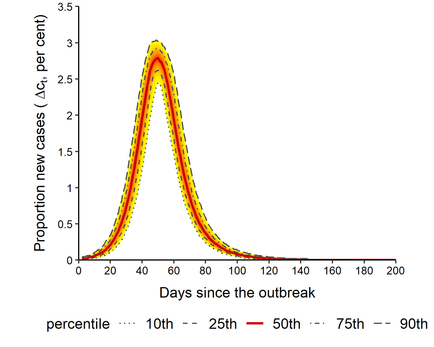
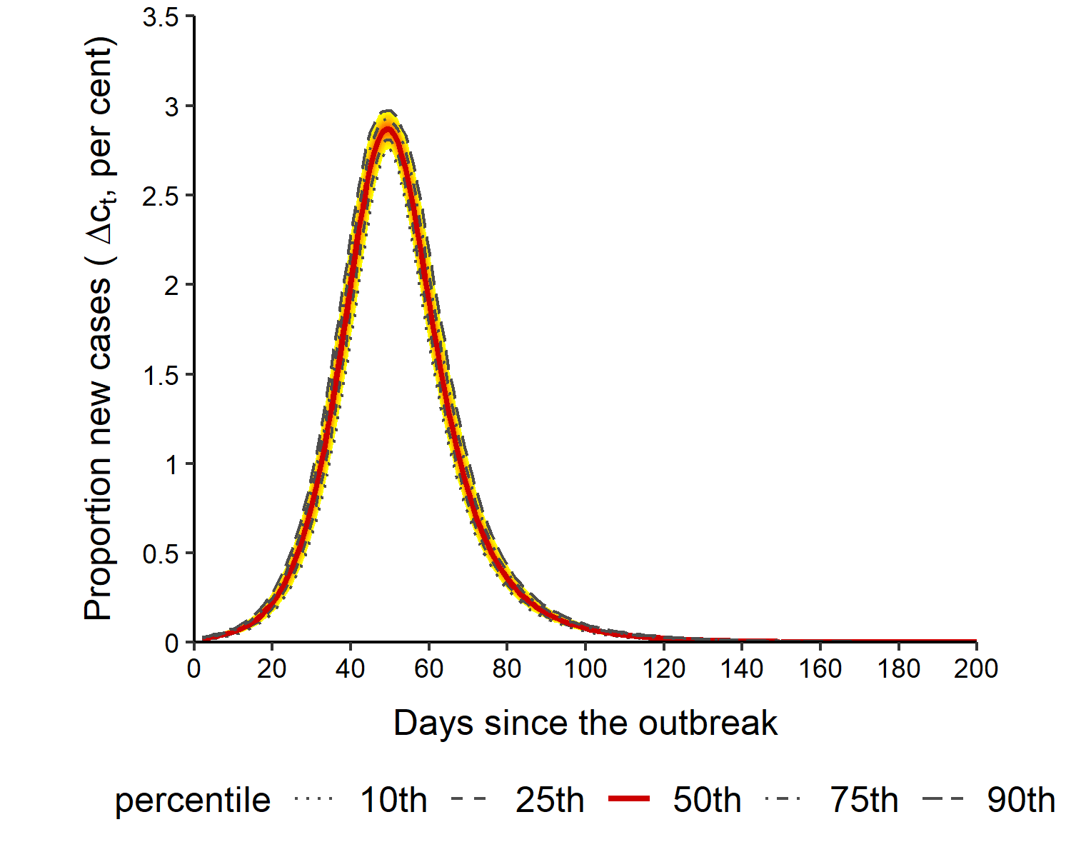
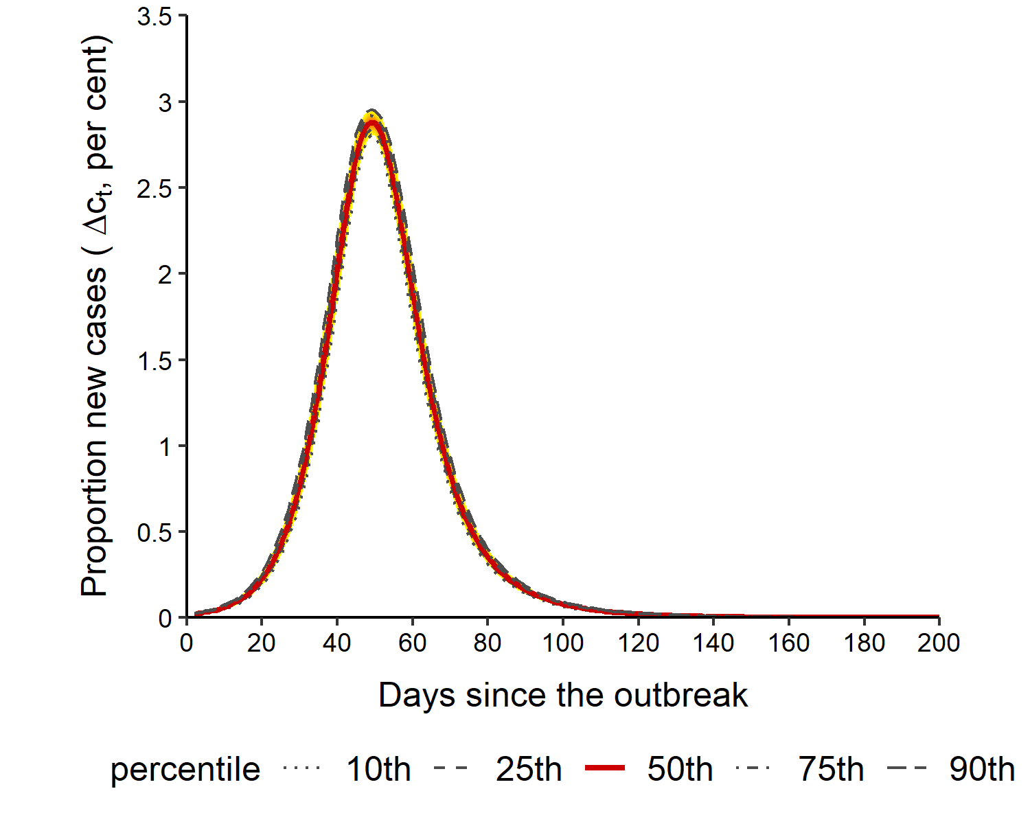
Notes: We set $1/1000$ of the population randomly infected on day $1$ and use the Erdős-Rényi random network with mean contact number $k=10$. The recovery rate is $\gamma=1/14$. The exposure intensity parameter is $\tau=\gamma\mathcal{R}_{0}/k$. $c^{\ast}=B^{-1}\sum_{b=1}^{B}\max_{t}c_{t}^{(b)}=0.94$ in all three cases. The number of replications is $B=1,000$.

Figure S.2 compares the simulated aggregate new cases averaged over $1,000$ replications obtained by the single group model and the multigroup model with five age groups detailed in Section 5 of the main paper. What stands out in the figure is the similarity of the epidemic outcomes, including the peak of new cases, the maximum proportion of infected, and the duration of the epidemic. This result suggests that the aggregate outcomes do not seem to be affected by the number of groups used in the simulations.

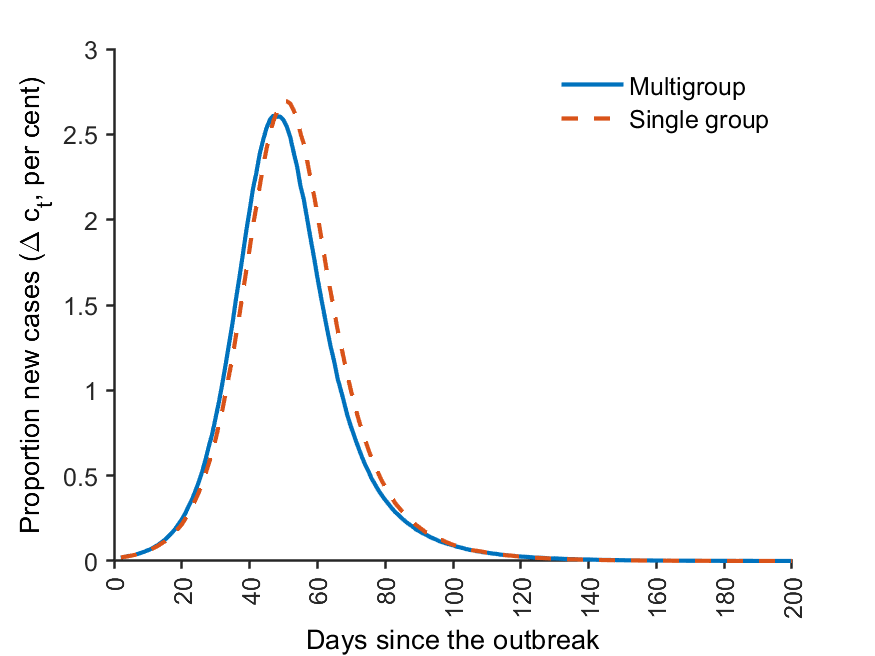
Figure S.2: The average number of aggregate new cases using the single- and multi-group models with ${\mathcal{R}_{0}}=3$

Notes: The average proportion of new cases over $1,000$ replications is displayed. The average number of new cases is very close to the median, although not shown. Population size is $n=10,000$.  In the case of a single group, the Erdős-Rényi random network with mean contact number $k=10$ was used. $c^{\ast}=B^{-1}\sum_{b=1}^{B}\max_{t}c_{t}^{(b)}=0.94$, and the duration of the epidemic is $T^{\ast}=212$ days. In the case of the multigroup model, $c^{\ast}=0.90$, and $T^{\ast}=215$ days.

We next examine the effect of network topology on the simulation results. In particular, we consider two widely used random networks – the Erdős-Rényi (ER) and the power law random networks. For simplicity, we examine the single group model. Recall that in an ER random graph, each pair of the nodes are connected at random with a uniform probability $p=k/\left(n-1\right)$. In the limit of large $n$ (with the mean degree $k$ fixed), the ER random network has a Poisson degree distribution, which may depart from real-world contact networks in which a small number of individuals (such as school-aged children, medical professionals, delivery drivers, and sales workers) may have a relatively high number of daily contacts. In other words, the degree distribution of the contact networks may be heavy-tailed (right-skewed). The power law random network is a popular choice to model this phenomenon. In a (truncated) power law graph, the degree distribution follows the power-law distribution:

$$p_{x}=Cx^{-\alpha},\text{ \ \ }x=k_{\min},k_{\min}+1,\ldots,k_{\max},$$ (S.8)

where $p_{x}$ is the fraction of nodes in the graph with degree $x$, $k_{\min}$ ($k_{\max}$) is the minimum (maximum) degree, $\alpha>1$ is a constant known as the power law exponent, and $C$ is a normalization constant such that $\sum_{k_{\min}}^{k_{\max}}p_{x}=1$. Figure S.3 illustrates the two networks with $n=50$ nodes and the same average degree, $k=10$. It is assumed that the minimum and maximum degrees of the power law network are $k_{\min}=5$ and $k_{\max}=49$, respectively. The networks were generated following the algorithms described in Section S3.1 of this online supplement. It can be seen from the figure that most nodes in the ER random network have comparable degrees with the mean degree of $10$ approximately. In contrast, the power law network has a heavy-tailed degree distribution, and there are many small-degree nodes as well as a few highly connected nodes in the graph.

Figure S.4 compares the simulation results obtained using the two random networks with the same average degree of $10$. We set $k_{\min}=5$ and $k_{\max}=50$ for the power law networks. The values of $\gamma$, $\mathcal{R}_{0}$, and $\tau$, and initialization of the simulation process are as given above. We plot the proportion of new cases with uncertainty bands and the mean values across $1,000$ replications for easy comparison. It is clear from Figure S.4 that the mean epidemic curves obtained by the two different random networks overlap. Although not shown, the median simulation results are very close to the mean values for both types of networks. We therefore focus on using the random network in our simulation and calibration exercises.

Figure S.3: Examples of Erdos-Renyi and power law networks

Erdős-Rényi random network		(Truncated) power law network

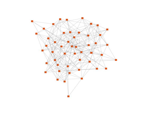
Notes: $n=50.$ Mean degree is $k=10$ in both networks. The degree distribution in the power law network follows $p_{x}=Cx^{-2.43},$ for $x=5,6,\ldots,49.$

Figure S.4: Simulated number of new cases using a single group model with ${\mathcal{R}_{0}}=3$ under different network topologies

Random network	Power law network	Comparison of means

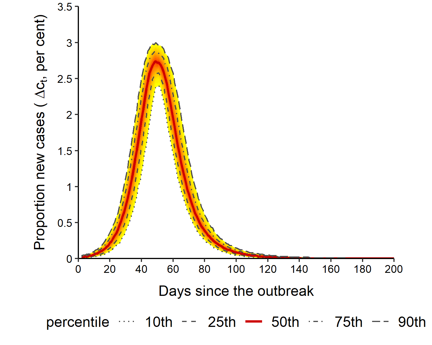
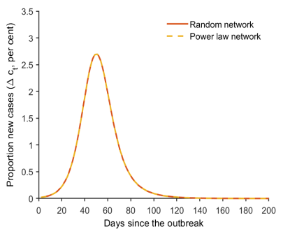
Notes: We set $1/1000$ of the population randomly infected on day $1$. Both networks have mean degrees $k=10$. The recovery rate is $\gamma=1/14$. The exposure intensity parameter is $\tau=\gamma\mathcal{R}_{0}/k$. Population size is $n=10,000$. $c^{\ast}=B^{-1}\sum_{b=1}^{B}\max_{t}c_{t}^{(b)}=0.94$ using both networks. The number of replications is $B=1,000.$

Appendix S4 Estimation of transmission and recovery rates

S4.1 Estimation of transmission rates

This section first provides further evidence on the performance of the rolling estimators of the transmission rates assuming no measurement errors, and then describes the method that estimates the transmission rate and the multiplication factor jointly. Table S.1, which complements Table 1 in the main paper, reports the finite sample properties of the 3-weekly rolling estimates of $\mathcal{R}_{0}$ in the case where it is fixed at $\mathcal{R}_{0}=3$. The simulated data were obtained under the same set-up as that for Table 1, and are based on a single group model with the random network and the parameter values $k=10$, $\gamma=1/14$, and $\beta=3/14$. Table S.1 presents the bias and root mean square error (RMSE) of the rolling estimates, $\mathcal{\hat{R}}_{0}\left(W\right)=\hat{\beta}_{t}\left(W\right)/\gamma$, where the window size $W=3$ weeks, and $\hat{\beta}_{t}\left(W\right)$ is computed based on (49) of the main paper. The results refer to averages computed over the four non-overlapping $3$-weekly sub-samples covering the $4^{th}-15^{th}$ weeks since the outbreak.

As to be expected, the bias remains small and similar over different sub-samples. The RMSE is smaller in the middle of the epidemic than at the beginning and end stages, where $i_{t}$ is very close to zero. Overall, the average RMSE of $\mathcal{\hat{R}}_{0}$ is reasonably small compared to the true value of $3$. Compared with Table 1 of the main paper, the properties of the $2$-weekly and $3$-weekly rolling estimates are very close, with the $3$-weekly rolling estimates having slightly smaller RMSE than the $2$-weekly estimates.

Table S.1: Finite sample properties of the 3-weekly rolling estimates of $\mathcal{R}_{0}$, in the case where it is fixed at ${\mathcal{R}_{0}}=3$

		3-weekly sub-samples
Weeks since the outbreak		$4^{th}-6^{th}$	$7^{th}-9^{th}$	$10^{th}-12^{th}$	$13^{th}-15^{th}$
Population
$n=10,000$	Bias	-0.0119	-0.0037	-0.0024	0.0026
	RMSE	0.0966	0.0488	0.0737	0.1687
$n=50,000$	Bias	-0.0019	-0.0002	-0.0009	-0.0005
	RMSE	0.0395	0.0218	0.0332	0.0750
$n=100,000$	Bias	-0.0003	0.0005	0.0000	-0.0006
	RMSE	0.0275	0.0150	0.0229	0.0544

Next, to allow for time-varying under-reporting of cases, Section 6.2 of the main paper proposes a method that jointly estimates the transmission rate and the multiplication factor (MF). Here we give detailed steps for the joint estimation. Let $\tilde{c}^{0}$ denote a small threshold value and $\hat{m}_{\left(j\right)}$ denote the $j^{th}$ estimate of MF, for $j=1,2,\ldots$. We propose the following algorithm.

• In the initial period of the epidemic when $\tilde{c}_{t}\leq\tilde{c}^{0}$, $t=1,2,\ldots,t^{0}$, carry out the rolling estimation of $\beta_{t}$ with a guess value of MF. Then simulate the stochastic network model using the $\left\{\hat{\beta}_{t}\right\}_{t=1}^{t^{0}}$, and compute the first estimate of MF as the ratio of the mean calibrated cases to realized cases at the end of the initial period, namely, $\hat{m}_{\left(1\right)}=\bar{c}_{t^{0}}/\tilde{c}_{t^{0}}$, where $\bar{c}_{t^{0}}=B^{-1}\sum_{b=1}^{B}c_{t^{0}}^{\left(b\right)}.$

• When $\tilde{c}_{t}>\tilde{c}^{0}$, we jointly estimate $\beta_{t}$ and $m_{t}$ by the two equations below:

  $$\hat{\beta}_{t}\left(W_{\beta}\right)=\text{Argmin}_{\beta}\sum_{\tau=t-W_{\beta}+1}^{t}\left[\frac{1-\hat{m}_{\tau}(W_{m})\tilde{c}_{\tau}}{1-\hat{m}_{\tau-1}(W_{m})\tilde{c}_{\tau-1}}-e^{-\beta\text{ }\hat{m}_{\tau-1}(W_{m})\tilde{\imath}_{\tau-1}}\right]^{2}.$$ (S.9)

  $$\hat{m}_{t}(W_{m})=\frac{W_{m}^{-1}\sum_{\tau=t-W_{m}+1}^{t}\left(1-B^{-1}\sum_{b=1}^{B}e^{-\hat{\beta}_{\tau-1}\left(W_{\beta}\right)\text{ }i_{\tau-1}^{\left(b\right)}}\right)}{W_{m}^{-1}\sum_{\tau=t-W_{m}+1}^{t}\left[\tilde{c}_{\tau}-\left(B^{-1}\sum_{b=1}^{B}e^{-\hat{\beta}_{\tau-1}\left(W_{\beta}\right)\text{ }i_{\tau-1}^{\left(b\right)}}\right)\tilde{c}_{\tau-1}\right]},$$ (S.10)

  where $W_{\beta}$ and $W_{m}$ are the rolling window sizes. Specifically,

  • From $t^{0}+1$ to $t_{2}=t^{0}+W_{m}$, carry out rolling estimation of $\beta_{t}$ by (S.9) using $\hat{m}_{\left(1\right)}$. Then continue the simulations using $\left\{\hat{\beta}_{t}\right\}_{t=t^{0}+1}^{t_{2}}$ from the stored status, and compute $\hat{m}_{\left(2\right)}$ by (S.10) at $t_{2}$.

  • From $t_{2}+1$ to $t_{3}=t_{2}+W_{m}$, carry out rolling estimation of $\beta_{t}$ by (S.9) using $\hat{m}_{\left(2\right)}$. Then continue the simulations using $\left\{\hat{\beta}_{t}\right\}_{t=t_{2}+1}^{t_{3}}$ and compute $\hat{m}_{\left(3\right)}$ by (S.10) at $t_{3}$.

  • Continue the above steps to obtain $\hat{m}_{\left(4\right)}$, $\hat{m}_{\left(5\right)}$, $\ldots,$ until the end of the sample.

In practice, MF varies slowly, and it is reasonable to consider $W_{\beta}=W_{m}=2$ or $3$ weeks. We apply the above procedure to Covid-19 data in a number of European countries and the US. The results are presented in Section 7 of the main paper and Sections S5 and S6 of this supplement.

S4.2 Estimation of the recovery rate

As noted in the main paper, with reliable data on the number of removed (recovered or dead), the recovery rate, $\gamma$, can be estimated using the moment condition given by (29) of the main paper. In reality, however, it is hard to measure $R_{t}$ accurately. We do not estimate $\gamma$ in the calibration exercise because the data on recovery are either unavailable or problematic in the countries we considered. In the current section, we demonstrate that the recovery rate can be estimated very precisely using simulated data. To simplify the exposition, we consider a single group ($L=1$) and suppose that the time to recovery follows a geometric distribution as in the standard SIR model. The same aggregate outcome follows in the multigroup case if the probability of recovery is the same across all groups. Under these conditions, the aggregate moment condition for recovery can be written as

$$\Delta R_{t+1}=\gamma I_{t}+u_{n,t+1},$$ (S.11)

where $\Delta R_{t+1}=R_{t+1}-R_{t}$ and $u_{n,t+1}$ is a martingale difference process with respect to $I_{t}$ and $R_{t}$. ($I_{t}=C_{t}-R_{t}$). Recall from (5) and (6) of the main paper that $R_{t}=\sum_{i=1}^{n}y_{it}$ and $I_{t}=\sum_{i=1}^{n}z_{it}$, we note that $u_{n,t+1}$ is an aggregated error, namely, $u_{n,t+1}=\sum_{i=1}^{n}u_{i,t+1}.$ Dividing both sides of (S.11) by $n$ yields

$$\Delta r_{t+1}=\gamma i_{t}+\bar{u}_{n,t+1},$$ (S.12)

where $\Delta r_{t+1}=r_{t+1}-r_{t}$, $r_{t}=R_{t}/n$, $i_{t}=I_{t}/n$ and $\bar{u}_{n,t+1}=n^{-1}\sum_{i=1}^{n}u_{i,t+1}$. For sufficiently large $n$ and assuming that the individual differences in recovery are cross-sectionally weakly correlated, we have $\bar{u}_{t+1}=O_{p}(n^{-1/2})$. It follows that $\gamma$ can be consistently estimated from (S.12) by ordinary least squares (OLS) regression of $\Delta r_{t+1}$ on $i_{t}$. Note that $T$ is finite as $n\rightarrow\infty$. Due to the presence of $O_{p}\left(n^{-1/2}\right)$ in (S.12), it is expected that as $n$ increases, the randomness will diminish and estimates of $\gamma$ become increasingly precise. In the limit we would expect $\Delta r_{t+1}-\gamma i_{t}=O_{p}(n^{-1/2})$.

To examine the finite sample properties of the OLS estimator of $\gamma$, we simulate our model assuming a homogeneous recovery rate and compute the aggregate time series for $B=1,000$ replications under a given population size, $n$. Denote the recovery and infection time series of the $b^{th}$ replication by $r_{t+1}^{(b)}$ and $i_{t}^{(b)}$, respectively, for $b=1,2,\ldots,B.$ For each replication, we obtain $\hat{\gamma}^{(b)}$ by regressing $\Delta r_{t+1}^{(b)}$ on $i_{t}^{(b)}$, without an intercept. The true value of $\gamma$ in the experiment is set to $1/14$.

Table S.2: Finite sample properties of the rolling estimates of $\gamma$

		3-weekly sub-samples
Weeks since the outbreak		$4^{th}-6^{th}$	$7^{th}-9^{th}$	$10^{th}-12^{th}$	$13^{th}-15^{th}$
$2$-weekly rolling estimates
Population
$n=10,000$	Bias$\left(\times 100\right)$	0.0917	0.0111	0.0040	0.0072
	RMSE$\left(\times 100\right)$	0.9077	0.2465	0.1315	0.1833
$n=50,000$	Bias$\left(\times 100\right)$	0.0247	0.0006	0.0000	0.0023
	RMSE$\left(\times 100\right)$	0.3716	0.1034	0.0602	0.0840
$n=100,000$	Bias$\left(\times 100\right)$	0.0116	0.0012	-0.0002	0.0008
	RMSE$\left(\times 100\right)$	0.2536	0.0730	0.0430	0.0601
$3$-weekly rolling estimates
Population
$n=10,000$	Bias$\left(\times 100\right)$	0.0495	0.0082	0.0041	0.0067
	RMSE$\left(\times 100\right)$	0.5614	0.1681	0.1104	0.1639
$n=50,000$	Bias$\left(\times 100\right)$	0.0092	-0.0019	0.0005	0.0020
	RMSE$\left(\times 100\right)$	0.2302	0.0713	0.0511	0.0760
$n=100,000$	Bias$\left(\times 100\right)$	0.0055	0.0008	-0.0002	0.0009
	RMSE$\left(\times 100\right)$	0.1589	0.0512	0.0366	0.0542

Table S.2 reports the bias and RMSE of the OLS estimator of $\gamma$ averaged over the four non-overlapping $3$-weekly sub-samples during the $4^{th}-15^{th}$ weeks after the outbreak. Even though the bias and RMSE in the table have been multiplied by $100$, they are very small in magnitude. It is evident that we can estimate $\gamma$ very precisely even with short time series samples and population size $n=10,000$. The RMSE declines as $n$ increases, lending support to the theory. As in the case of estimating the transmission rates, the RMSEs are relatively larger in the early and late stages of the epidemic when $i_{t}$ is small. The 2-weekly and 3-weekly estimates are similar, with the 3-weekly estimator having some improvement as the outbreak amplifies into an epidemic.

Appendix S5 Estimates of the effective reproduction numbers

S5.1 Estimates for selected European countries

This section provides additional estimation results of the effective reproduction numbers ($\mathcal{R}_{et}$) and transmission rates ($\beta_{t}$) for the six European countries considered in the main paper. First, Figure S.5 presents the realized daily new cases (7-day average per $100,000$ people) and the 2-weekly rolling estimates of the transmission rates assuming a fixed MF $=3$ and $5$. It can be seen that the estimates of the transmission rate under different values of MF are virtually the same when $c_{t}$ is small. This observation clearly shows that MF is not identified in the early stage of the epidemic. It is also clear that the daily number of infections rapidly rises when $\beta_{t}$ is high.

Figure S.5: Realized new cases and two-weekly rolling estimates of the transmission rates for selected European countries

Austria
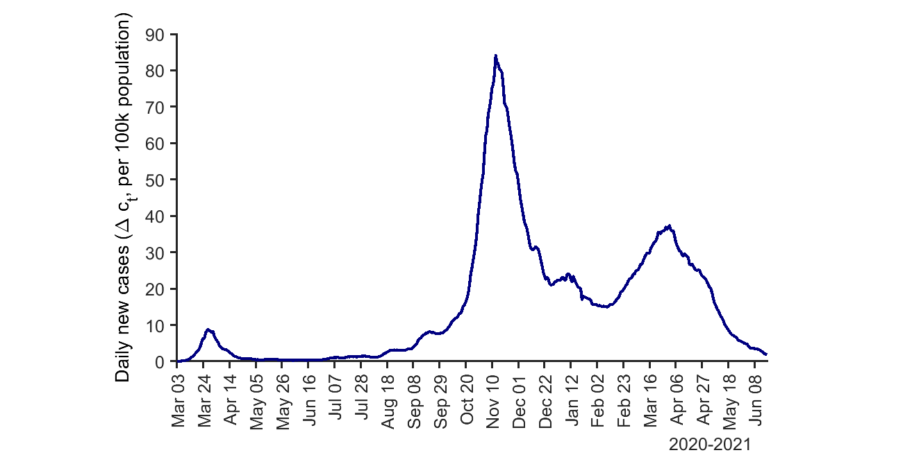
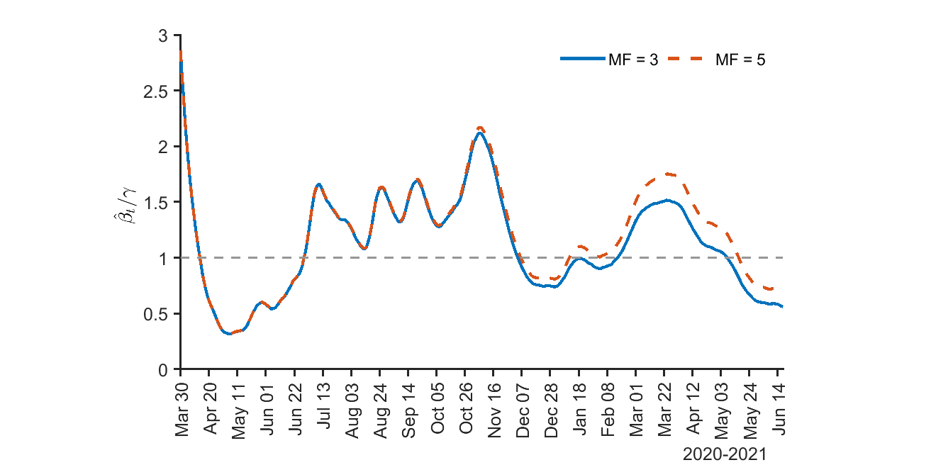
France
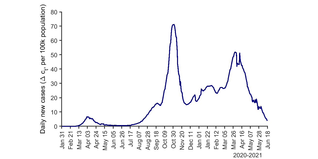
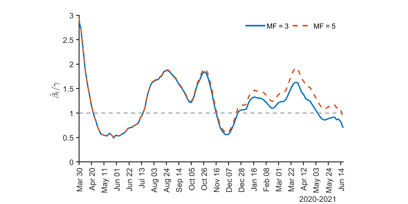
Germany

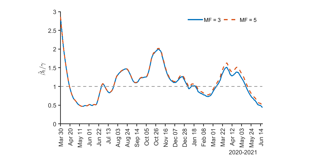
Notes: The figure plots the 7-day moving average of the reported number of new cases per 100k population and the 2-weekly rolling estimates of the transmission rate, $\beta_{t}/\gamma$, where $\gamma=1/14$ and the multiplication factor (MF) is fixed at $3$ and $5$.

Figure S.5: (Continued) Realized new cases and two-weekly rolling estimates of the transmission rate for selected European countries

Italy
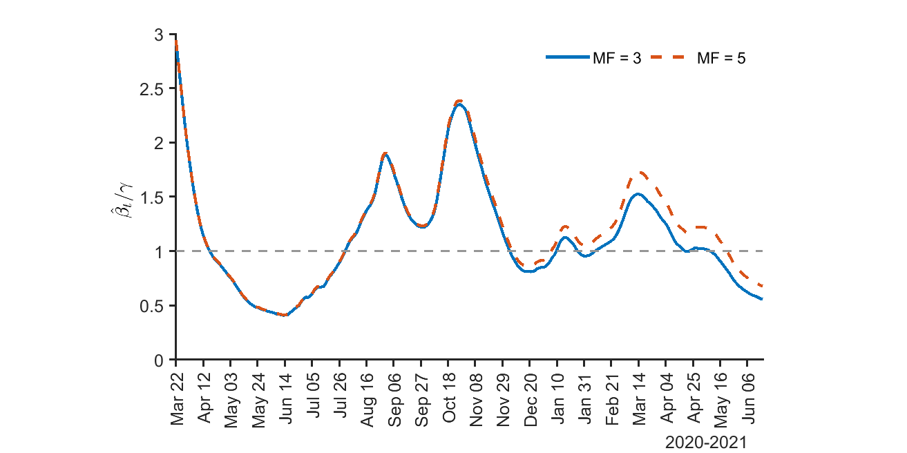
Spain
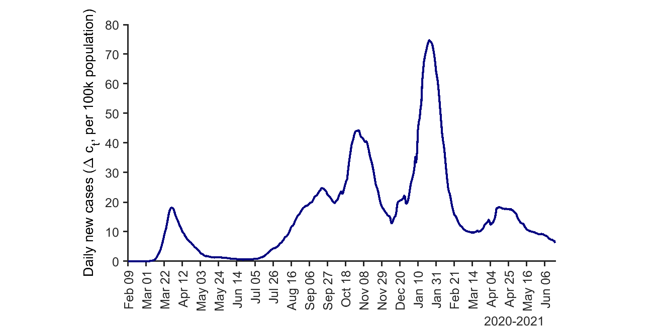
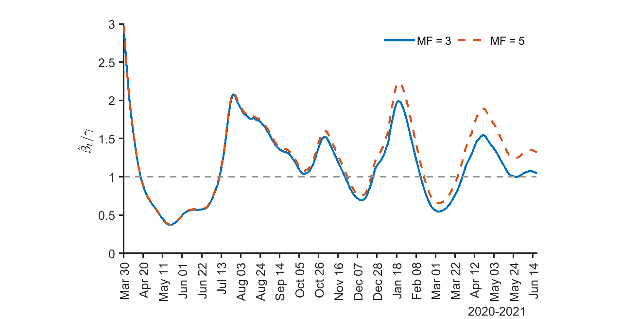
UK

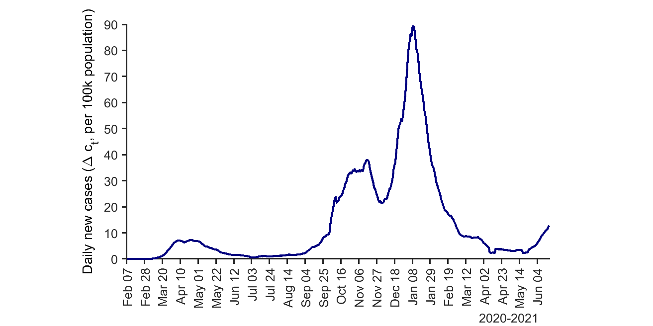
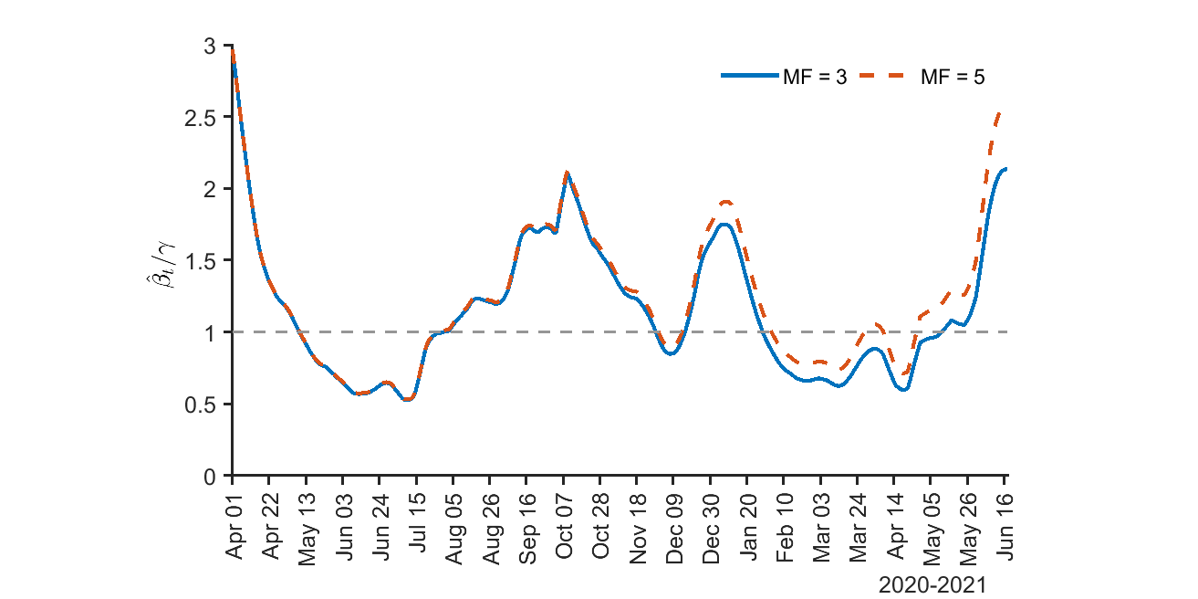
Figure S.6: Comparison of ${\hat{\mathcal{R}}_{et}}$ and ${\hat{\beta}_{t}}/{\gamma}$ for selected European countries

Austria		France
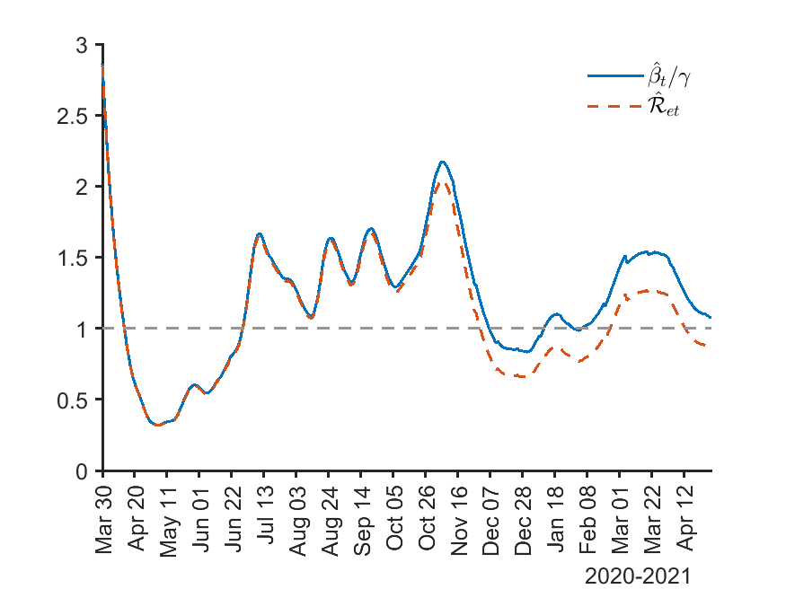
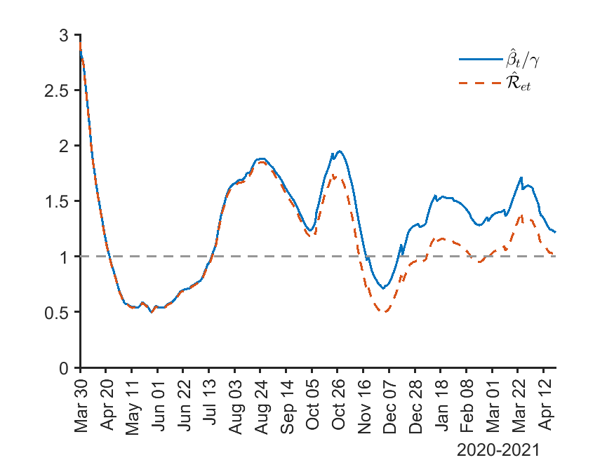
Germany		Italy
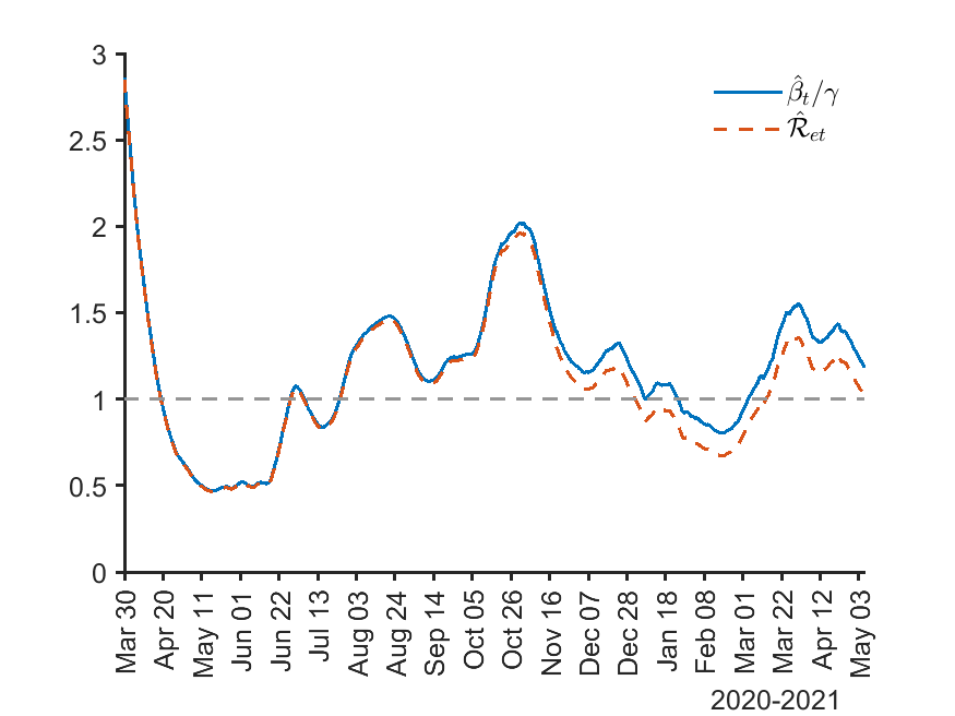
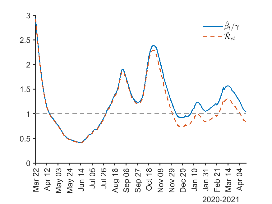
Spain		UK

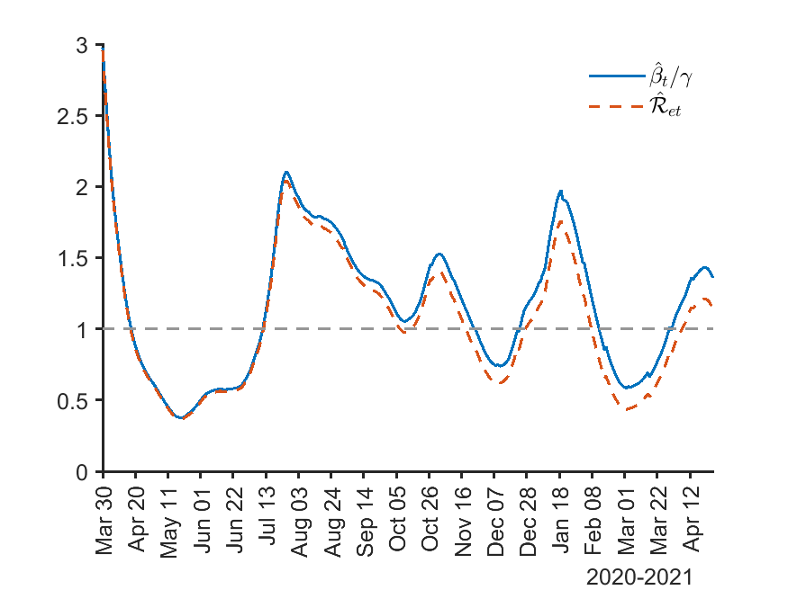
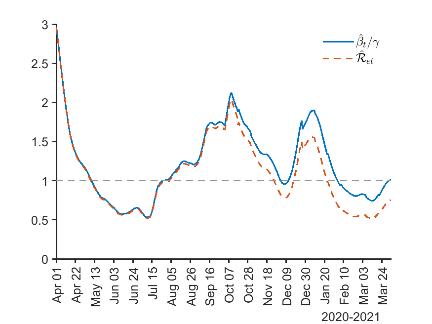
Notes: $\mathcal{\hat{R}}_{et}=\left(1-\hat{m}_{t}\tilde{c}_{t}\right)\hat{\beta}_{t}/\gamma$, where $\tilde{c}_{t}$ is the reported number of infections per capita and $\gamma=1/14$. $W_{\beta}=W_{m}=2$ weeks. The joint estimation starts when $\tilde{c}_{t}>0.01$. The initial guess estimate of the multiplication factor is $5$. The simulation uses the single group model with the random network and population size $n=50,000$. The number of replications is $500$. The number of removed (recoveries + deaths) is estimated recursively using $\tilde{R}_{t}=\left(1-\gamma\right)\tilde{R}_{t-1}+\gamma\tilde{C}_{t-1}$ for all countries, with $\tilde{C}_{1}=\tilde{R}_{1}=0$.

To illustrate the relationship between the transmission rate and the effective reproduction number, Figure S.6 plots $\hat{\beta}_{t}/\gamma$ together with $\mathcal{\hat{R}}_{et}=\left(1-\hat{m}_{t}\tilde{c}_{t}\right)\hat{\beta}_{t}/\gamma$ for the six countries, where $\hat{\beta}_{t}$ and $\hat{m}_{t}$ were estimated jointly using 2-weekly rolling windows. The values of $\mathcal{\hat{R}}_{et}$ and $\hat{m}_{t}$ are displayed in Figures 2 and 3 of the main paper. It is worth noting that $\mathcal{\hat{R}}_{et}$ is almost the same as $\hat{\beta}_{t}/\gamma$ in the early stage of the epidemic, since the proportion of infected is very small even after taking account of under-reporting. As infected cases grow, small differences between $\hat{\beta}_{t}/\gamma$ and $\mathcal{\hat{R}}_{et}$ start to become visible.

Figure S.7: Rolling estimates of the effective reproduction numbers ($\mathcal{R}_{et}$) using the 2- and 3-weekly rolling windows for selected European countries

Austria		France
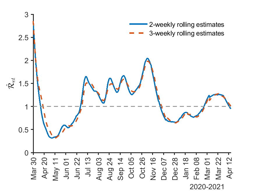
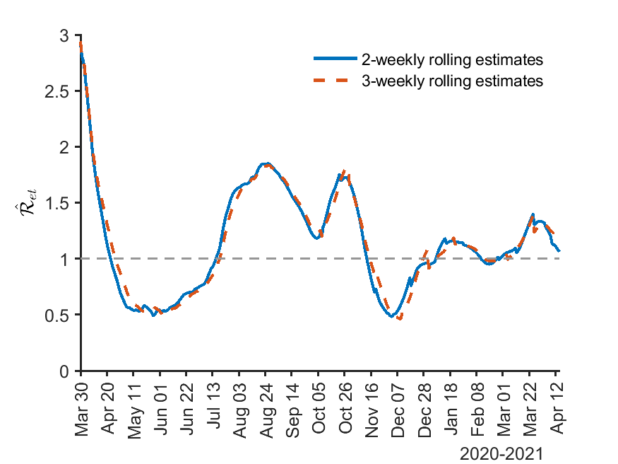
Germany		Italy
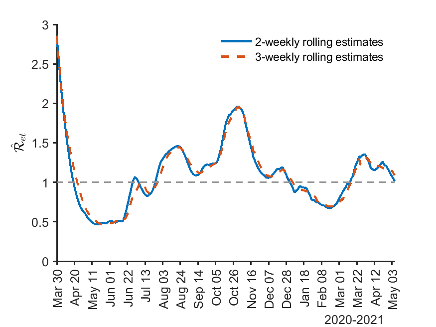
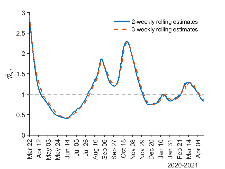
Spain		UK

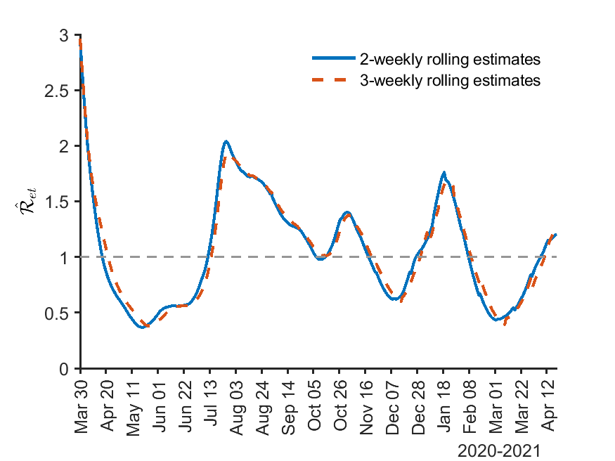
Notes: $\mathcal{\hat{R}}_{et}=\left(1-\hat{m}_{t}\tilde{c}_{t}\right)\hat{\beta}_{t}/\gamma$, where $\tilde{c}_{t}$ is the reported number of infections per capita and $\gamma=1/14$. $W_{\beta}=W_{m}=2$ and $3$ weeks. The joint estimation starts when $\tilde{c}_{t}>0.01$. The initial guess estimate of the multiplication factor is $5$. The simulation uses the single group model with the random network and population size $n=50,000$. The number of replications is $500$. The number of removed (recoveries + deaths) is estimated recursively using $\tilde{R}_{t}=\left(1-\gamma\right)\tilde{R}_{t-1}+\gamma\tilde{C}_{t-1}$ for all countries, with $\tilde{C}_{1}=\tilde{R}_{1}=0$.

Figure S.7 compares the 2- and 3-weekly rolling estimates of $\mathcal{R}_{et}$ obtained by the joint estimation procedure. It is apparent that using 2- and 3-weekly rolling windows produces very similar results. Therefore, our conclusions are unaltered if we adopt the 3-weekly estimates of the transmission rates in calibrating the model to the empirical evidence.

S5.2 Estimates for the US

It is also interesting to examine how the reproduction numbers have evolved in the US. This section presents estimates of $\mathcal{R}_{et}$ for the US at the country and state levels. Figure S.8 presents the reported daily new cases (per $100,000$ people) and the 2-weekly rolling estimates of $\mathcal{R}_{et}$ obtained by the joint estimation method for the US over the period of March 2020 to March 10, 2021 (when the share of the population fully vaccinated reached 10 percent). The results show that $\mathcal{\hat{R}}_{et}$ briefly dipped below $1$ in May and then again in August 2020. In contrast with the estimates in the European countries, $\mathcal{R}_{et}$ in the US never decreased to a level as low as $0.5$, resulting in a higher number of cases per capita.

Figure S.8: Realized new cases and two-weekly rolling estimates of the effective reproduction numbers ($\mathcal{R}_{et}$) for the US

Daily new cases		Estimates of $\mathcal{R}_{et}$

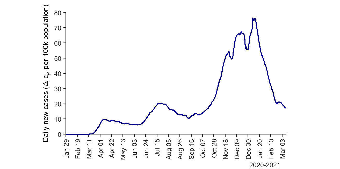
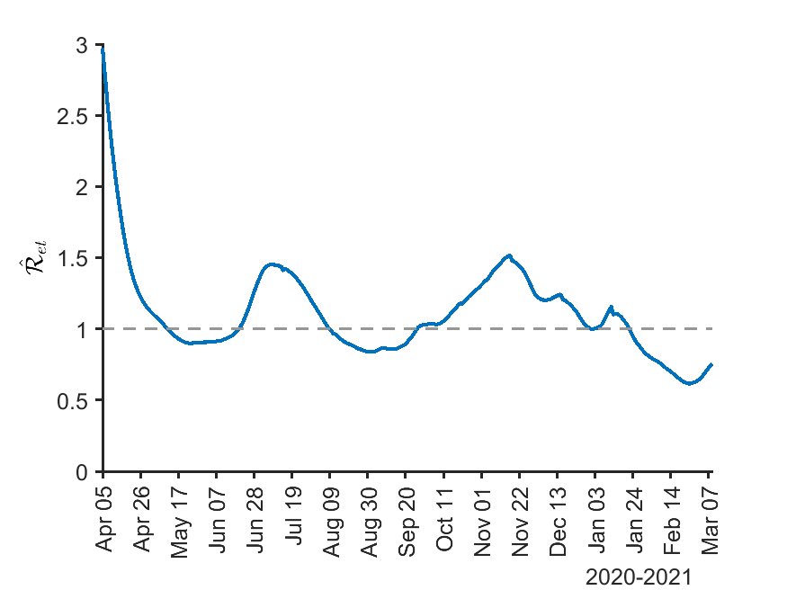
Notes: The reported daily new cases (7-day moving average) are displayed on the left. $\mathcal{\hat{R}}_{et}=\left(1-\hat{m}_{t}\tilde{c}_{t}\right)\hat{\beta}_{t}/\gamma$, where $\tilde{c}_{t}$ is the reported number of infections per capita and $\gamma=1/14.$ $W_{\beta}=W_{m}=2$ weeks. The joint estimation starts when $\tilde{c}_{t}>0.01$. The initial guess estimate of the multiplication factor is $5$. The simulation uses the single group model with population size $n=50,000$. The number of replications is $500$. The number of removed (recoveries + deaths) is estimated recursively using $\tilde{R}_{t}=\left(1-\gamma\right)\tilde{R}_{t-1}+\gamma\tilde{C}_{t-1}$, with $\tilde{C}_{1}=\tilde{R}_{1}=0$.

Figure S.9 presents the 2-weekly rolling estimates of $\mathcal{R}_{et}$ for the $48$ contiguous states and the District of Columbia over the period March 2020 to August 7, 2021. For simplicity, we used a fixed MF $=3$ in the estimation. It can be seen that the estimates share similar comovements but also display interesting patterns of heterogeneity across states. Overall, we observe that $\mathcal{R}_{et}$ rises above one around July and November 2020 and then increases quite rapidly again in July 2021 in most states. The peaks of the estimates were largely around $1.5$–$1.7$ in the first two hikes. In contrast, the latest surge in $\mathcal{R}_{et}$ was very rapid, reaching nearly two in most states in early August. This newest wave occurred right after many states had brought down $\mathcal{R}_{et}$ to $0.5$, the lowest level for many places in the US since the pandemic began.

Figure S.9: Two-weekly rolling estimates of the effective reproduction numbers ($\mathcal{R}_{et}$) for the contiguous US, by state

Alabama	Arizona
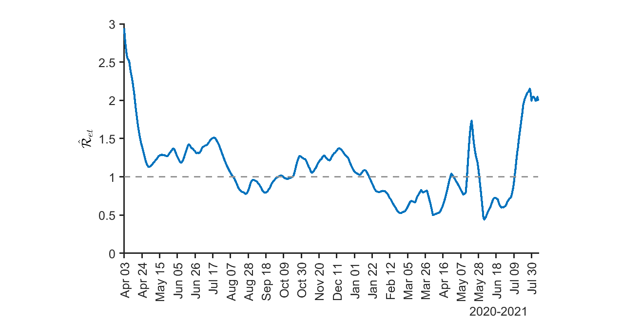
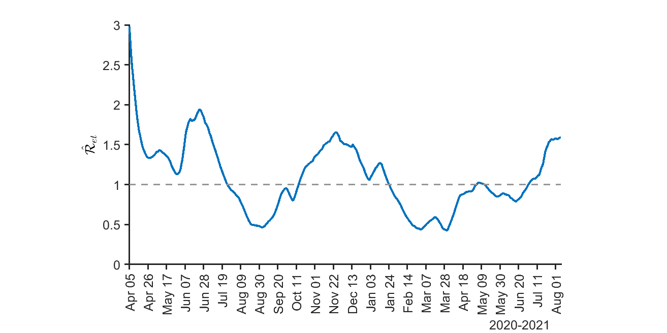
Arkansas	California
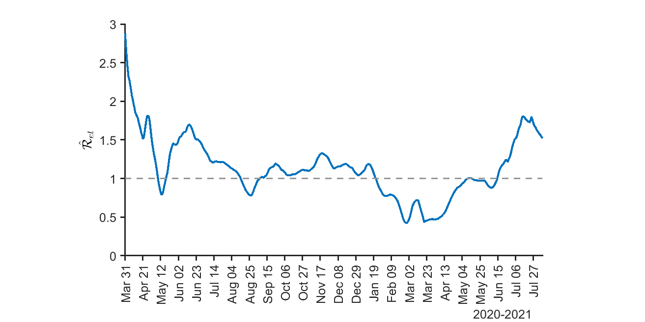
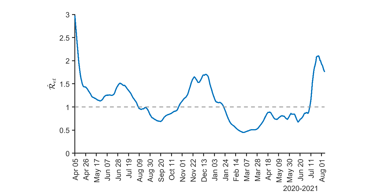
Colorado	Connecticut
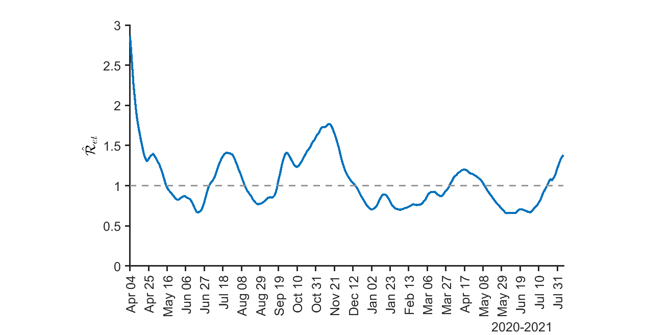
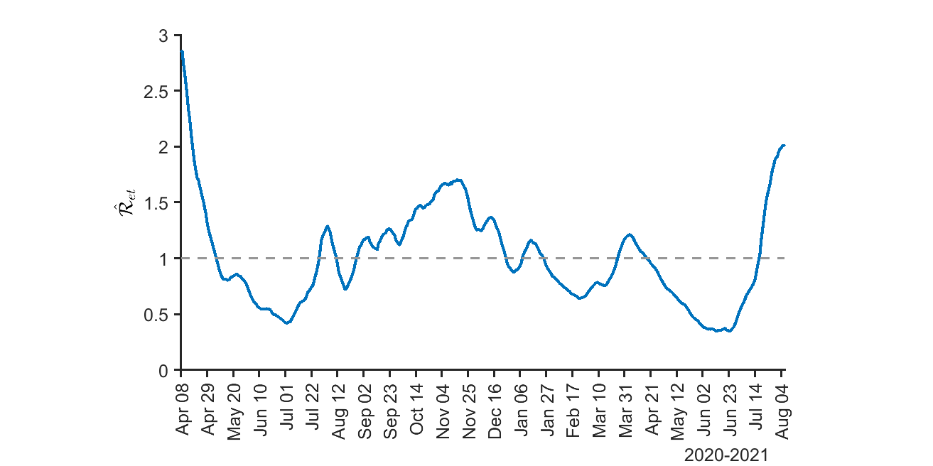
Delaware	District of Columbia

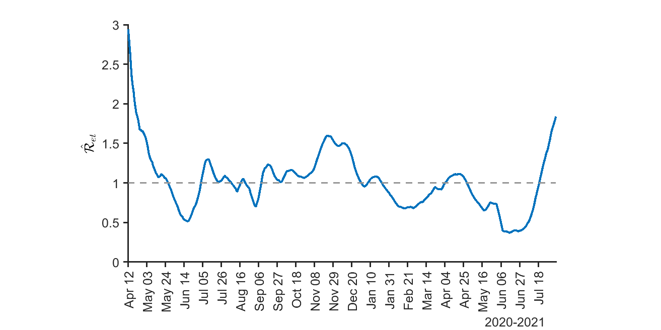
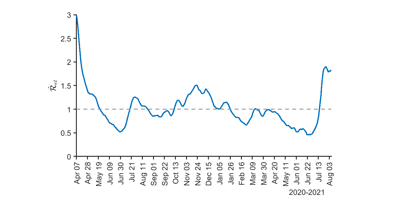
Notes: $\mathcal{\hat{R}}_{et}=\left(1-\text{MF}\tilde{c}_{t}\right)\hat{\beta}_{t}/\gamma$, where MF $=3$, $\tilde{c}_{t}$ is the reported number of infections per capita, and $\gamma=1/14$. The number of removed (recoveries + deaths) is estimated recursively using $\tilde{R}_{t}=\left(1-\gamma\right)\tilde{R}_{t-1}+\gamma\tilde{C}_{t-1}$ for all states, with $\tilde{C}_{1}=\tilde{R}_{1}=0$. Alabama included $306$, $4,877$, and $1,235$ backlogged cases on May 13–15, 2021.

Figure S.9: (Continued) Two-weekly rolling estimates of the effective reproduction numbers ($\mathcal{R}_{et}$) for the contiguous US, by state

Florida	Georgia
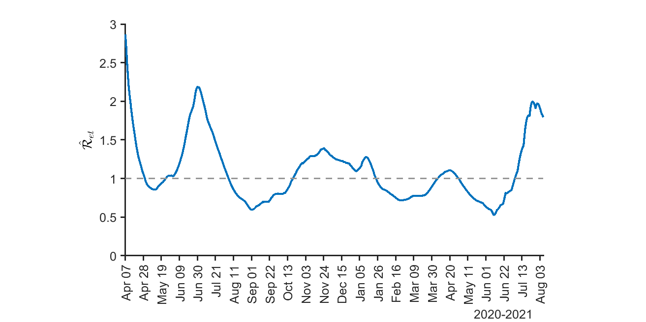
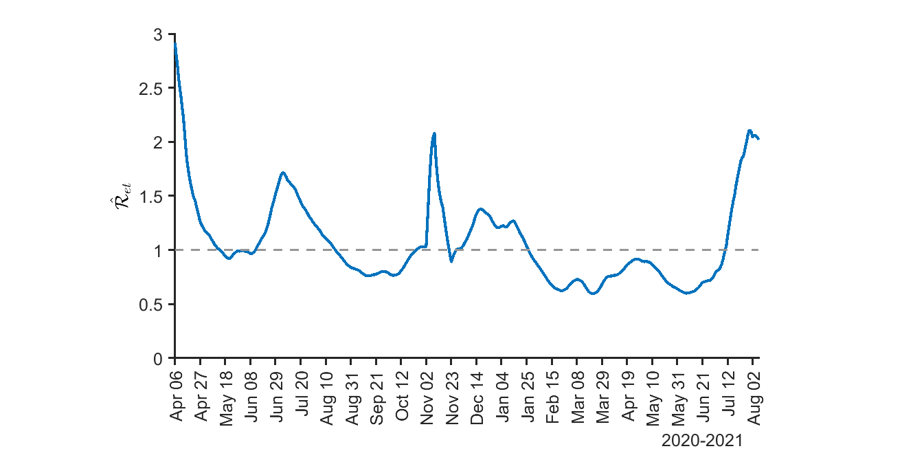
Idaho	Illinois
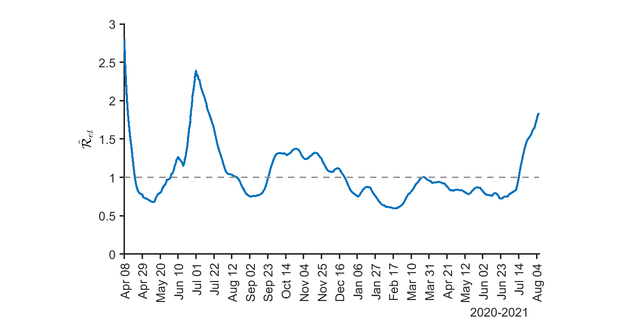
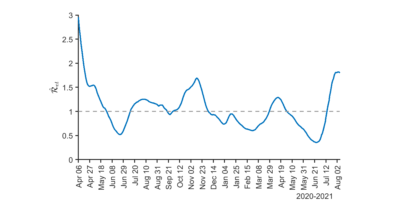
Indiana	Iowa
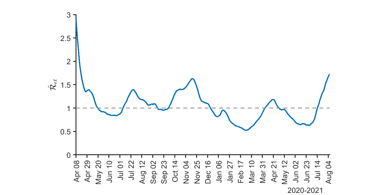
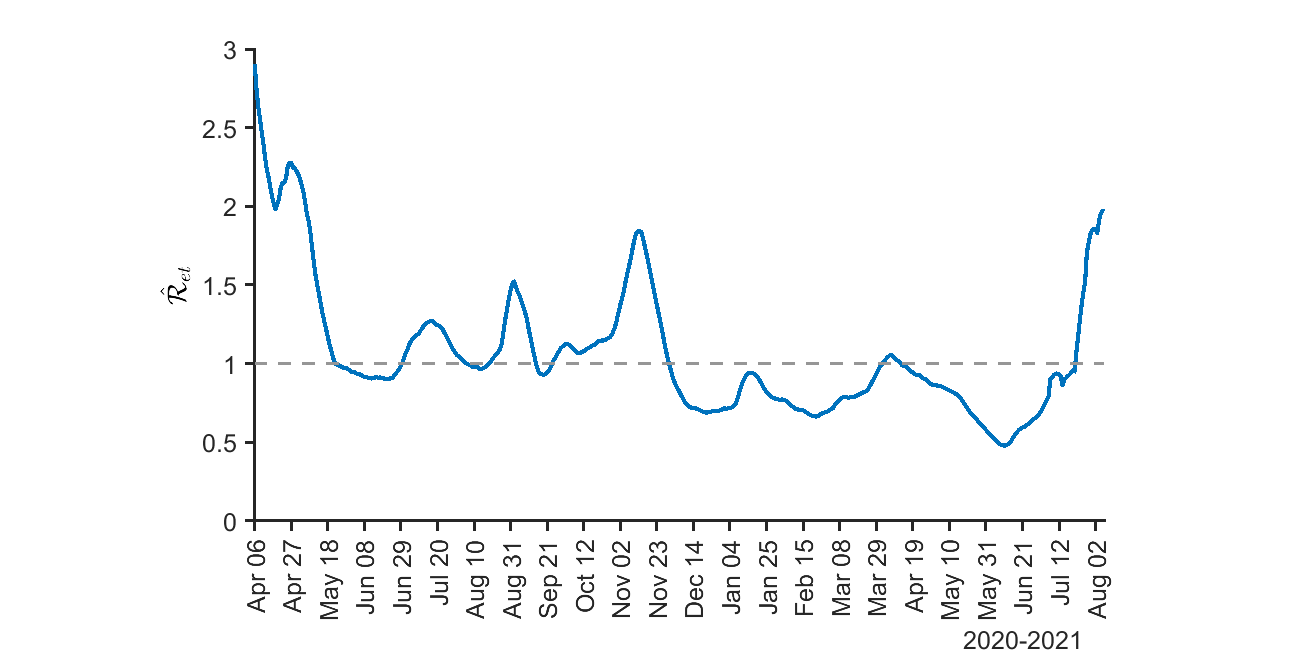
Kansas	Kentucky

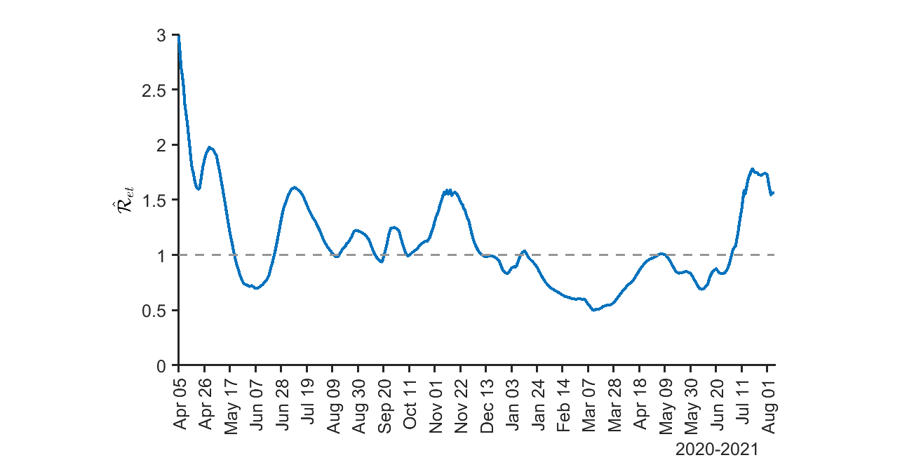
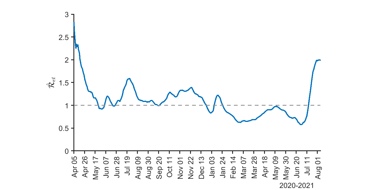
Notes: Florida stopped publishing daily case numbers on June 7, 2021. Georgia added $29,937$ antigen positive cases on November 3, 2020.

Figure S.9: (Continued) Two-weekly rolling estimates of the effective reproduction numbers ($\mathcal{R}_{et}$) for the contiguous US, by state

Louisiana	Maine
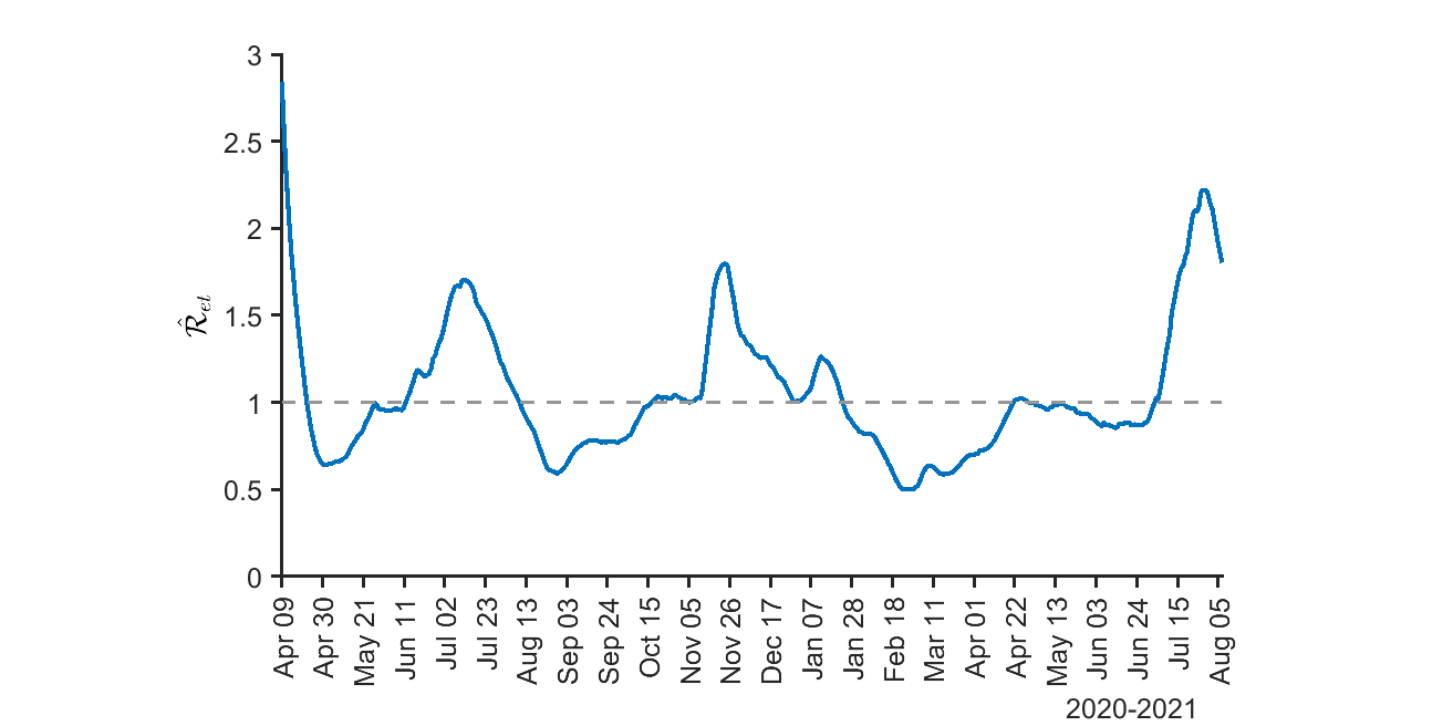
Maryland	Massachusetts
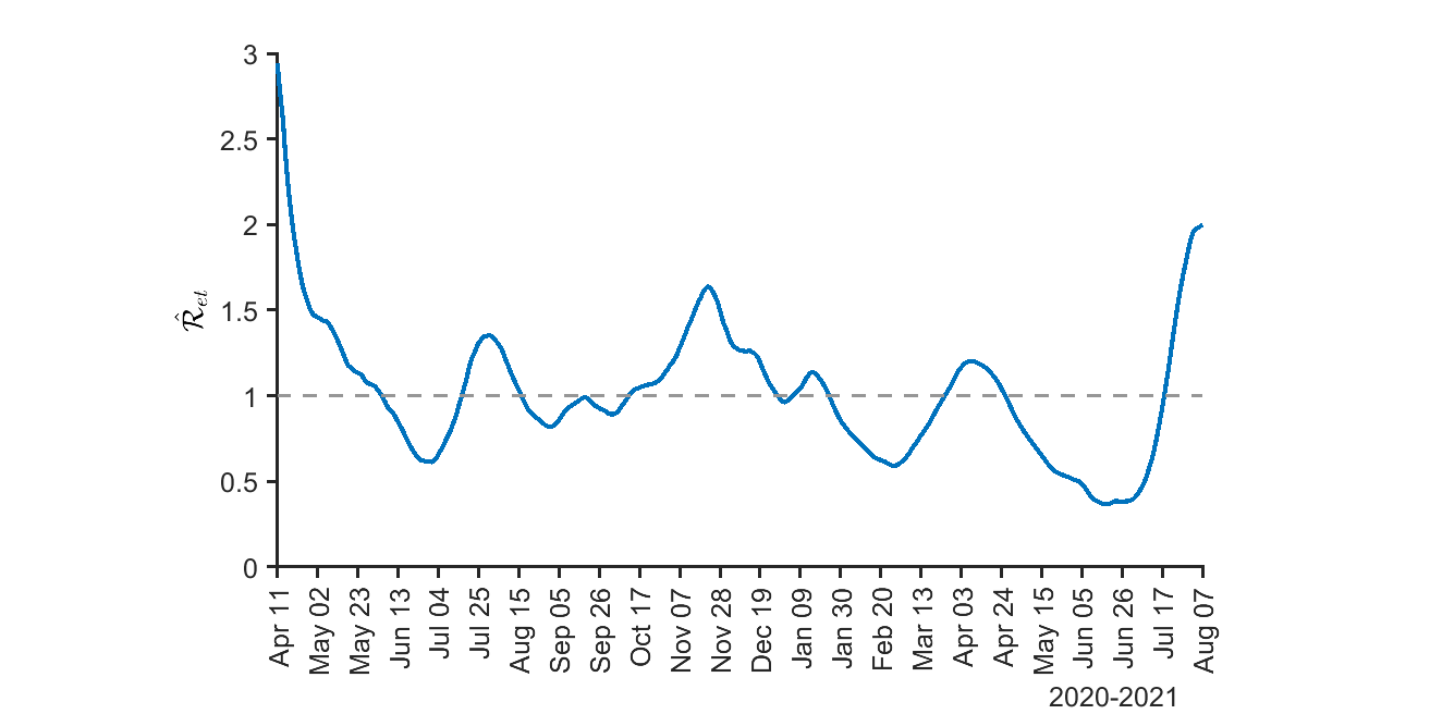
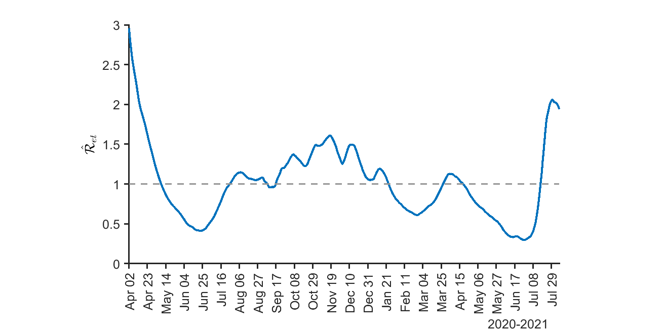
Michigan	Minnesota
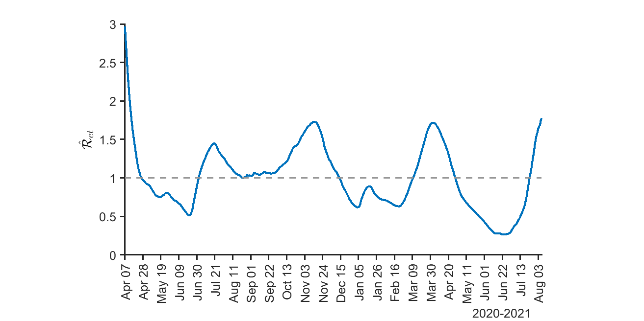
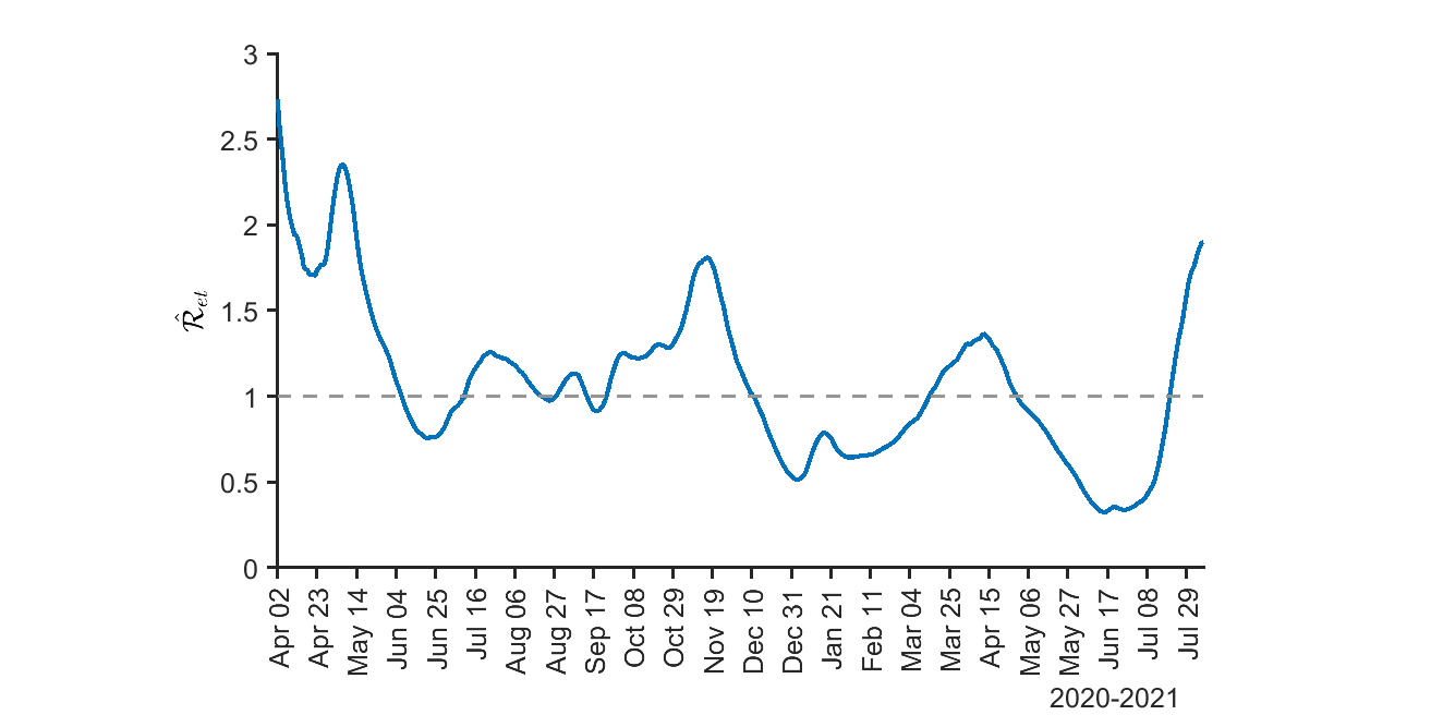
Mississippi	Missouri

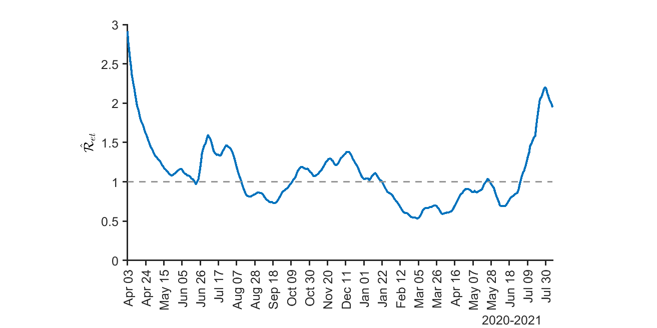
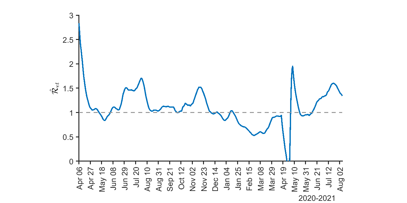
Notes: Missouri removed $11,454$ double counted cases on April 17, 2021.

Figure S.9: (Continued) Two-weekly rolling estimates of the effective reproduction numbers ($\mathcal{R}_{et}$) for the contiguous US, by state

Montana	Nebraska
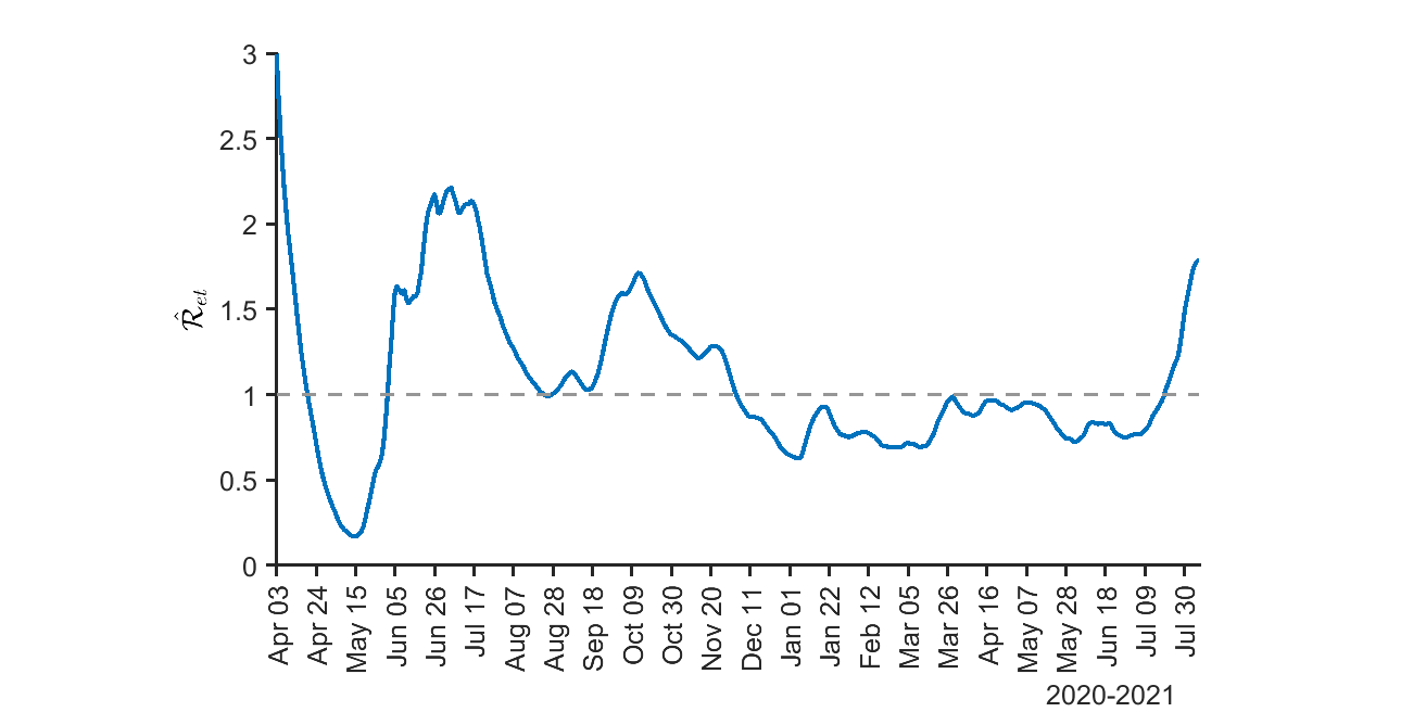
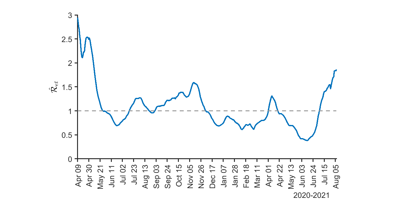
Nevada	New Hampshire
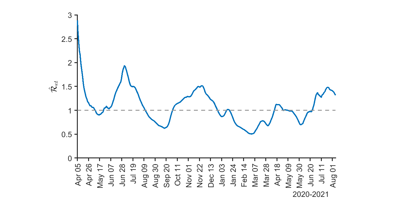
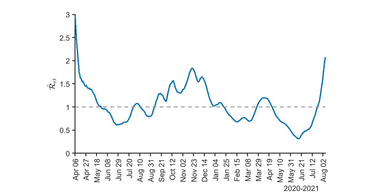
New Jersey	New Mexico
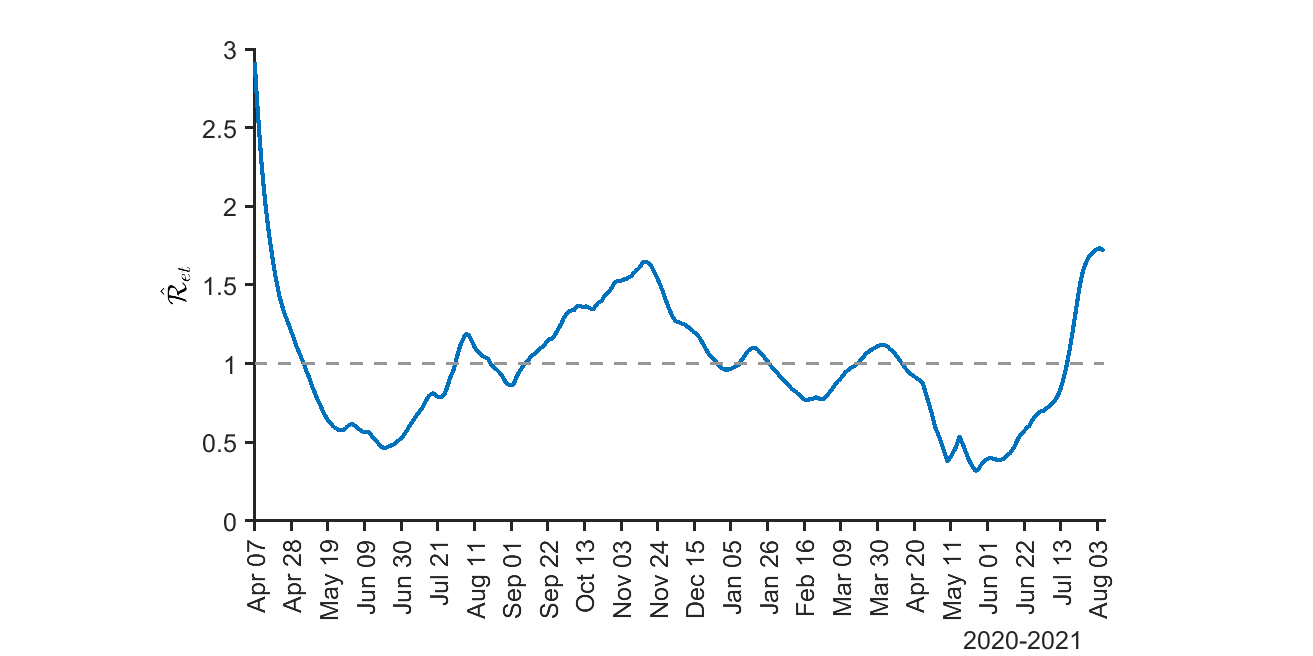
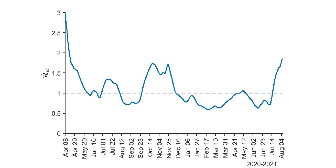
New York	North Carolina

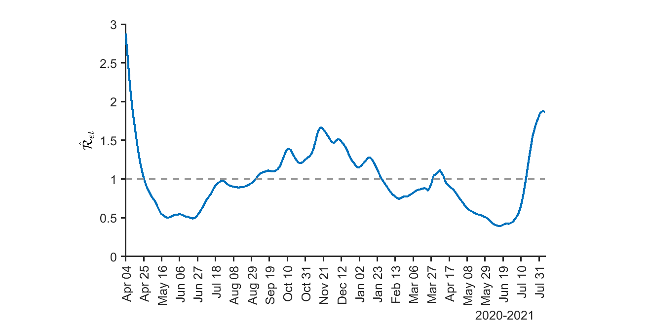
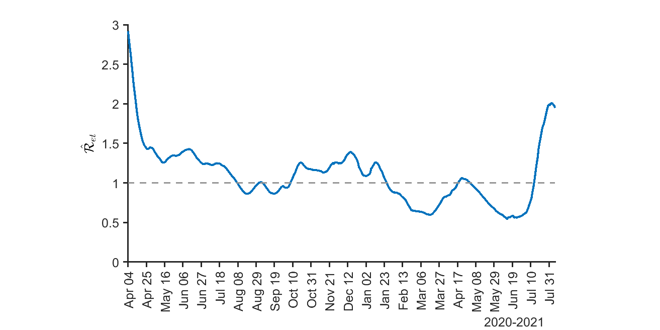
Figure S.9: (Continued) Two-weekly rolling estimates of the effective reproduction numbers ($\mathcal{R}_{et}$) for the contiguous US, by state

North Dakota	Ohio
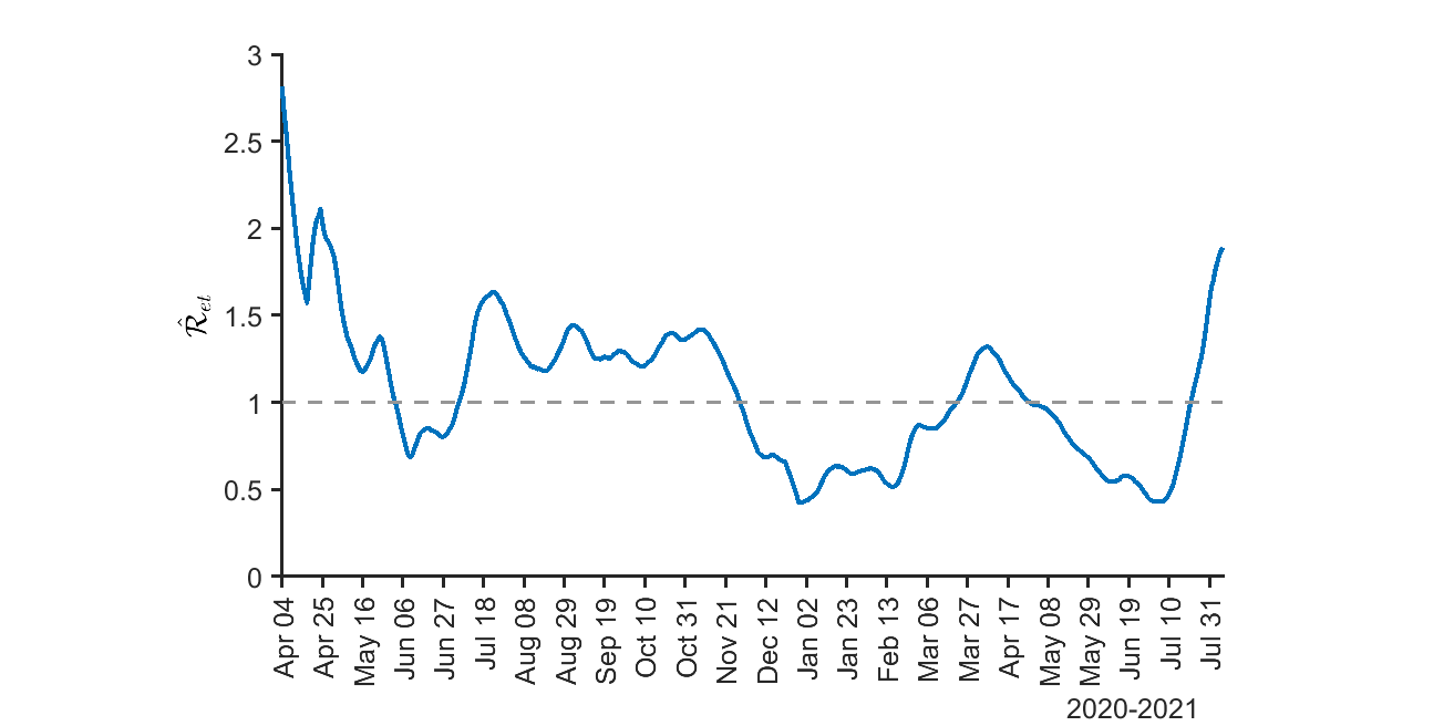
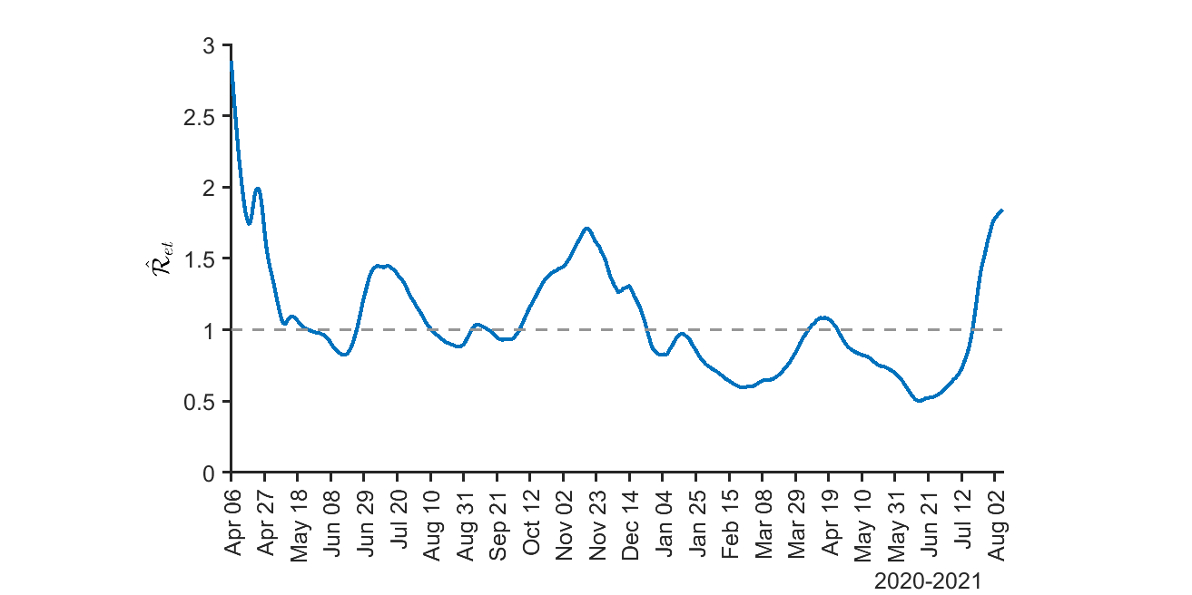
Oklahoma	Oregon
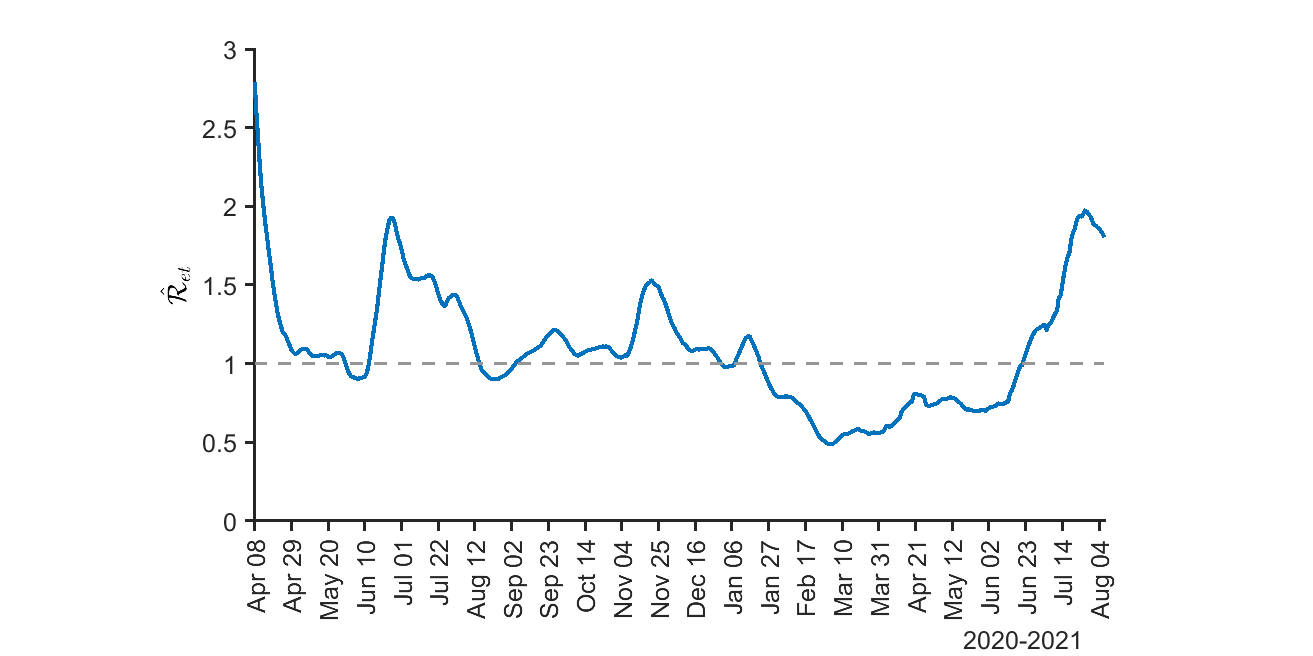
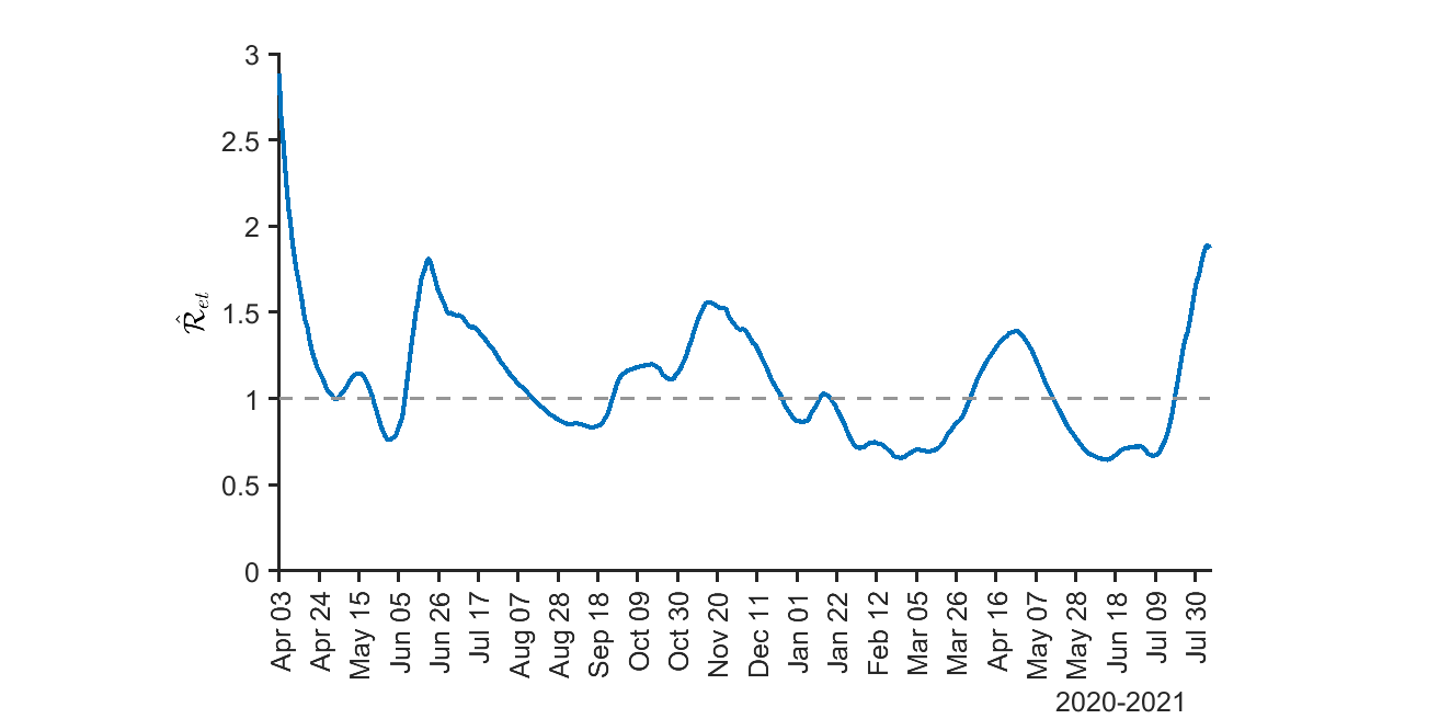
Pennsylvania	Rhode Island
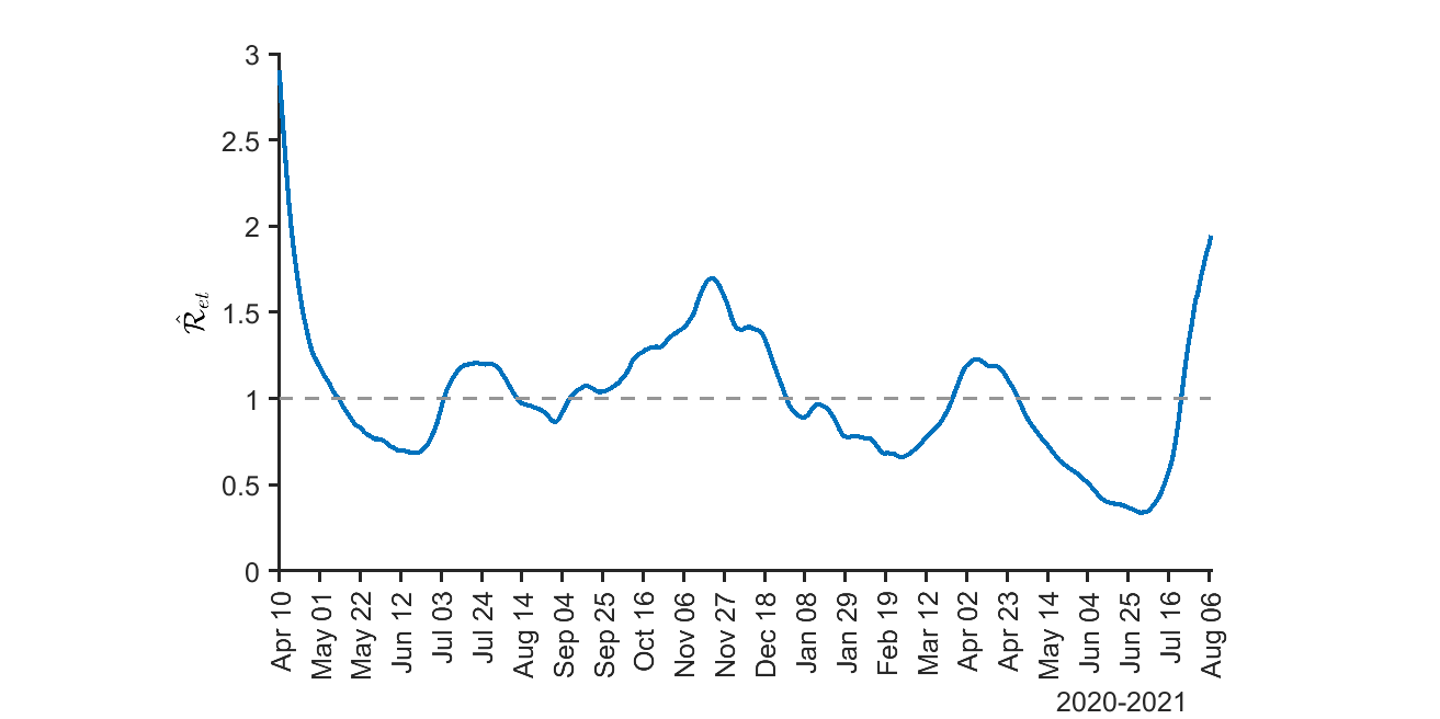
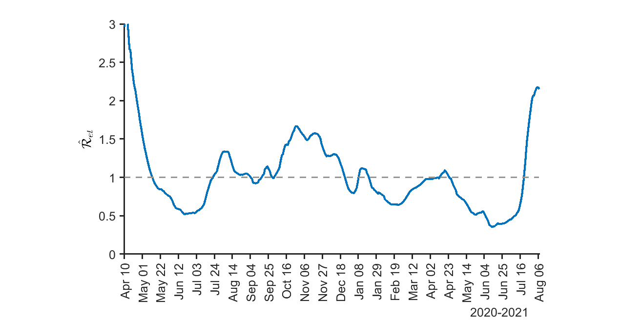
South Carolina	South Dakota

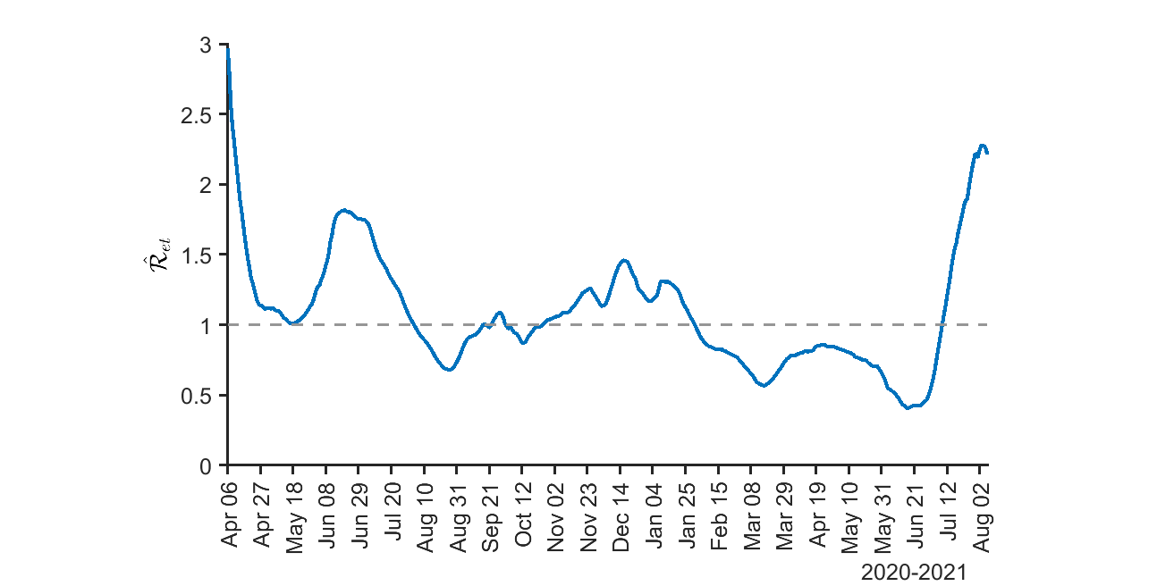
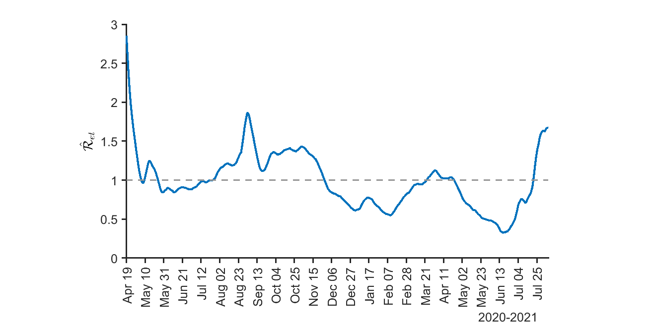
Notes: Ohio stopped publishing daily case numbers on June 2, 2021.

Figure S.9: (Continued) Two-weekly rolling estimates of the effective reproduction numbers ($\mathcal{R}_{et}$) for the contiguous US, by state

Tennessee	Texas
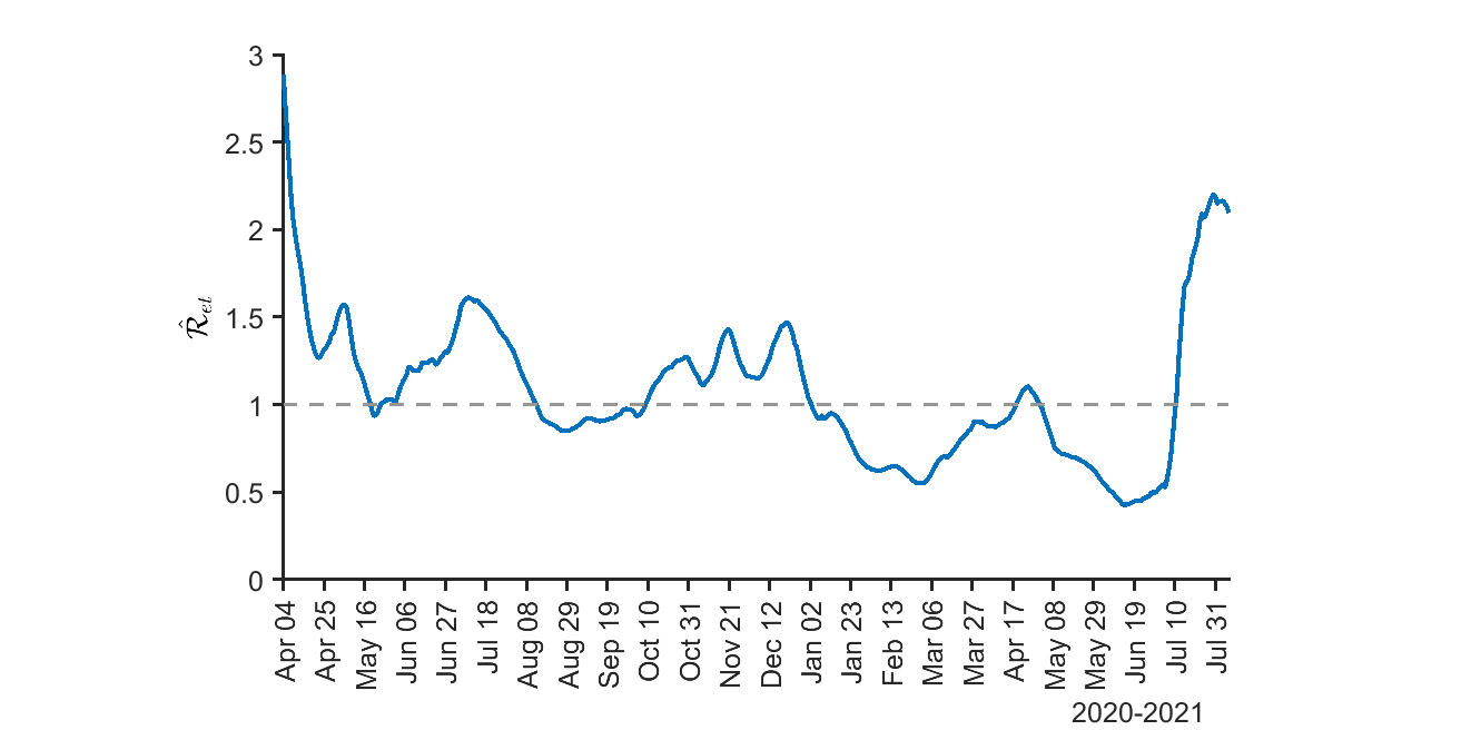
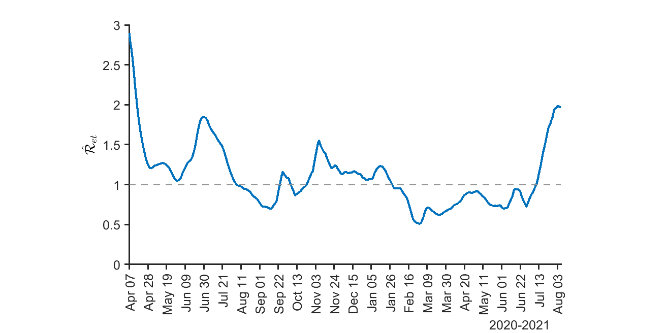
Utah	Vermont
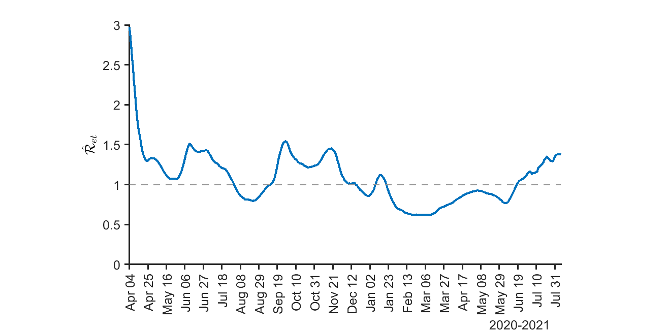
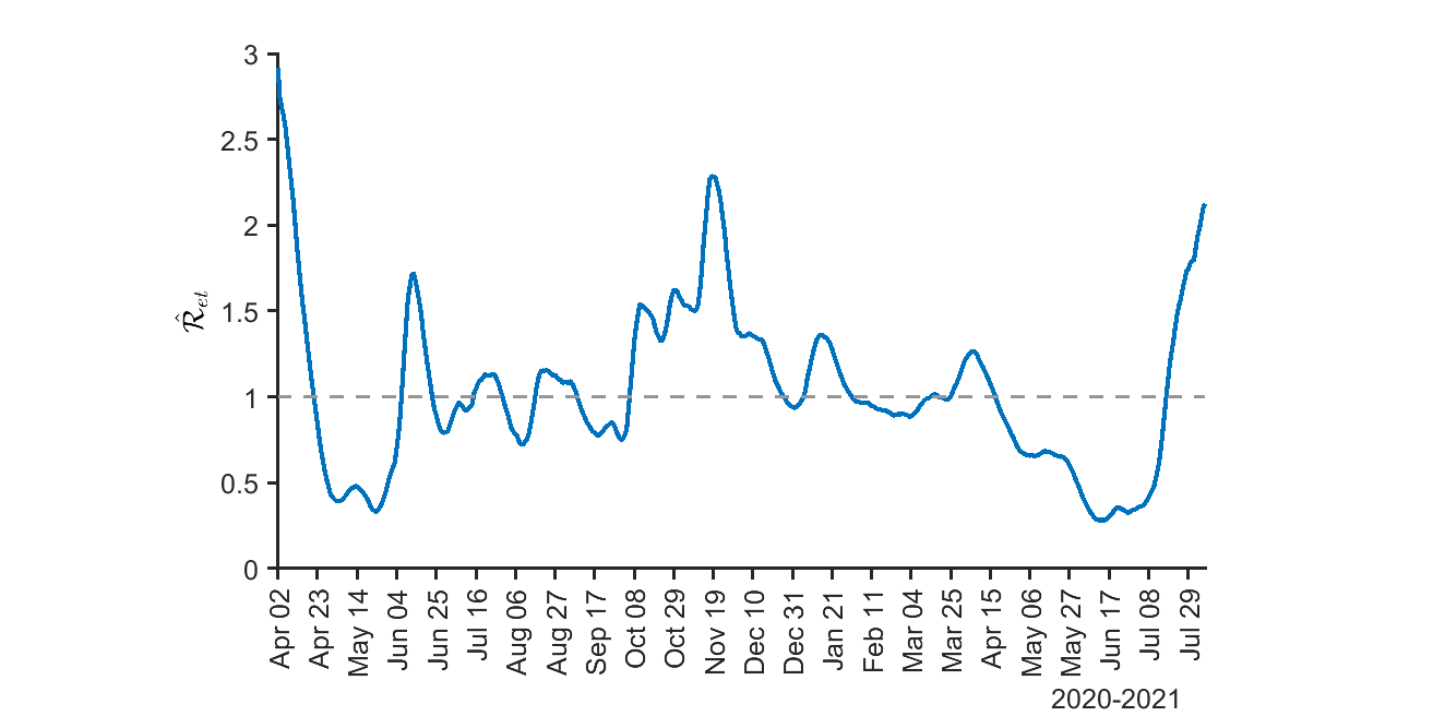
Virginia	Washington
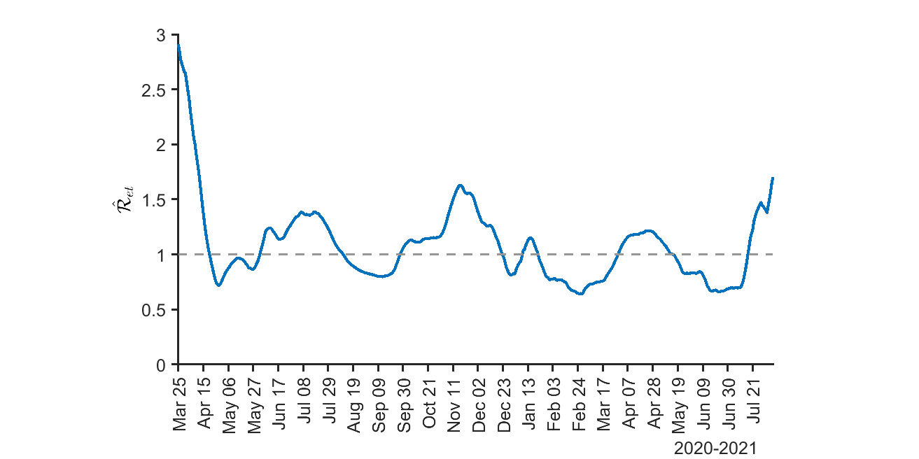
West Virginia	Wisconsin

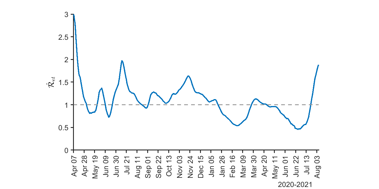
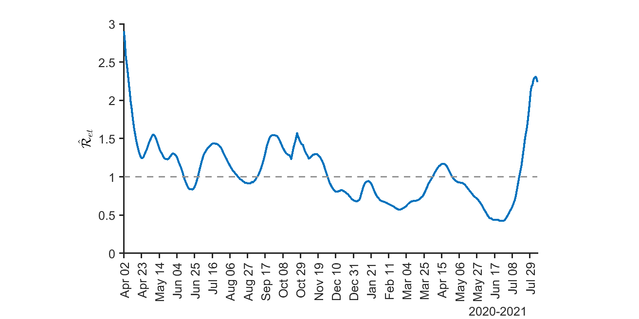
Figure S.9: (Continued) Two-weekly rolling estimates of the effective reproduction numbers ($\mathcal{R}_{et}$) for the contiguous US, by state

Wyoming

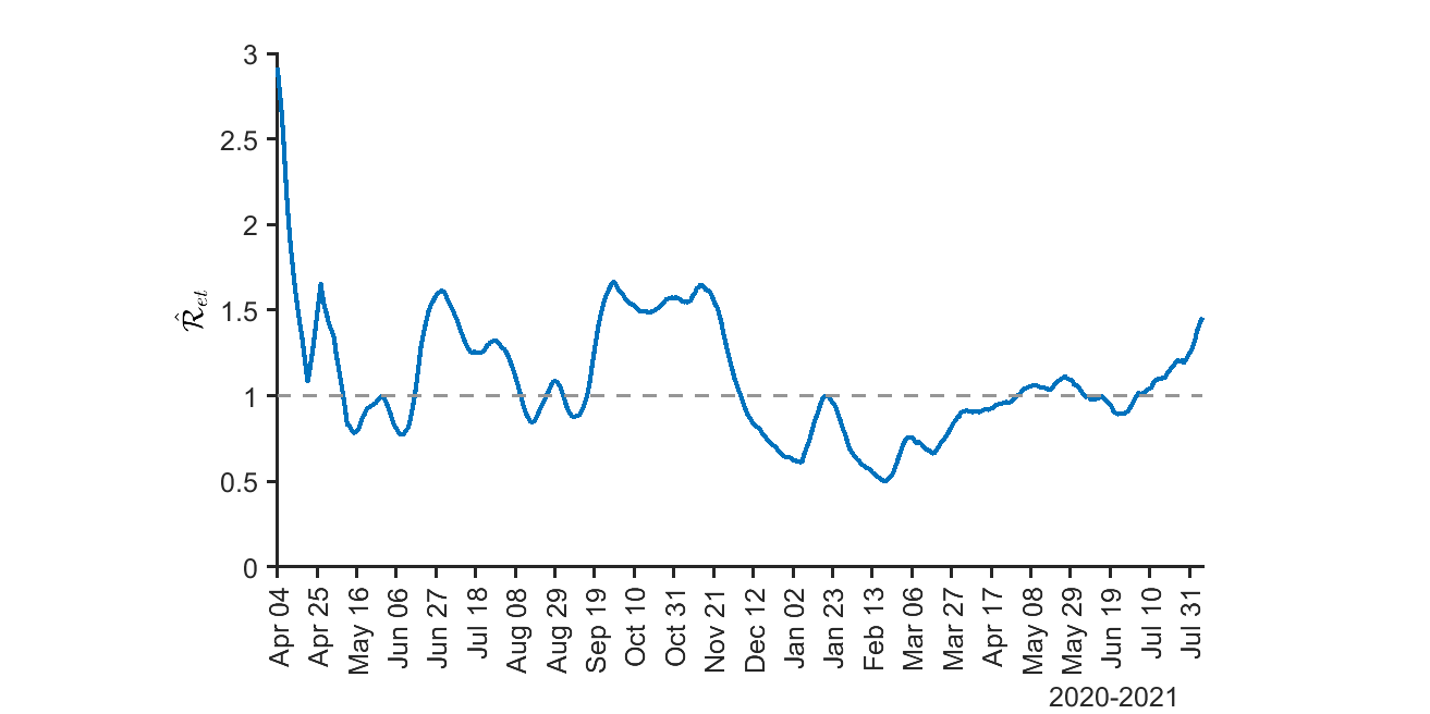
Appendix S6 Estimates of the multiplication factor

This section presents additional estimation results of the multiplication factor for the selected European countries and the US. It also compares the number of cases per capita with and without adjusting for under-reporting.

Figure S.10 compares the 2- and 3-weekly estimates of MF for the six European countries considered in the main paper. As the figure shows, the 3-weekly estimates of MF are slightly higher than the 2-weekly estimates. Still, overall they are very close and lead to negligible differences in the estimates of transmission rates, as we have seen in Figure S.7.

Figure S.10: Rolling estimates of the multiplication factor using the 2- and 3-weekly rolling windows for selected European countries

Austria		France
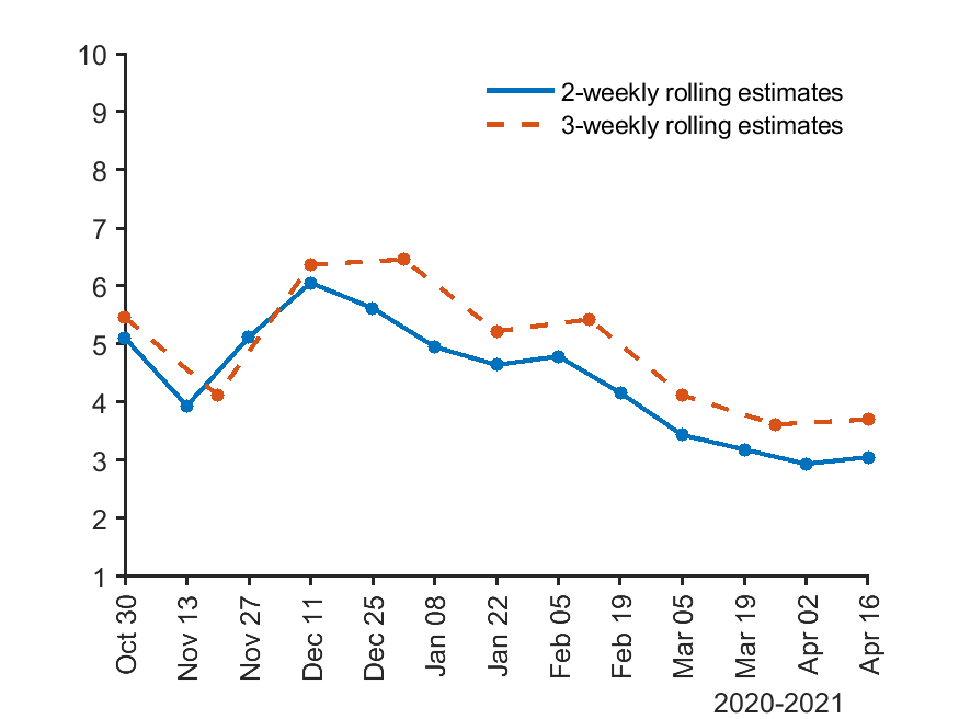
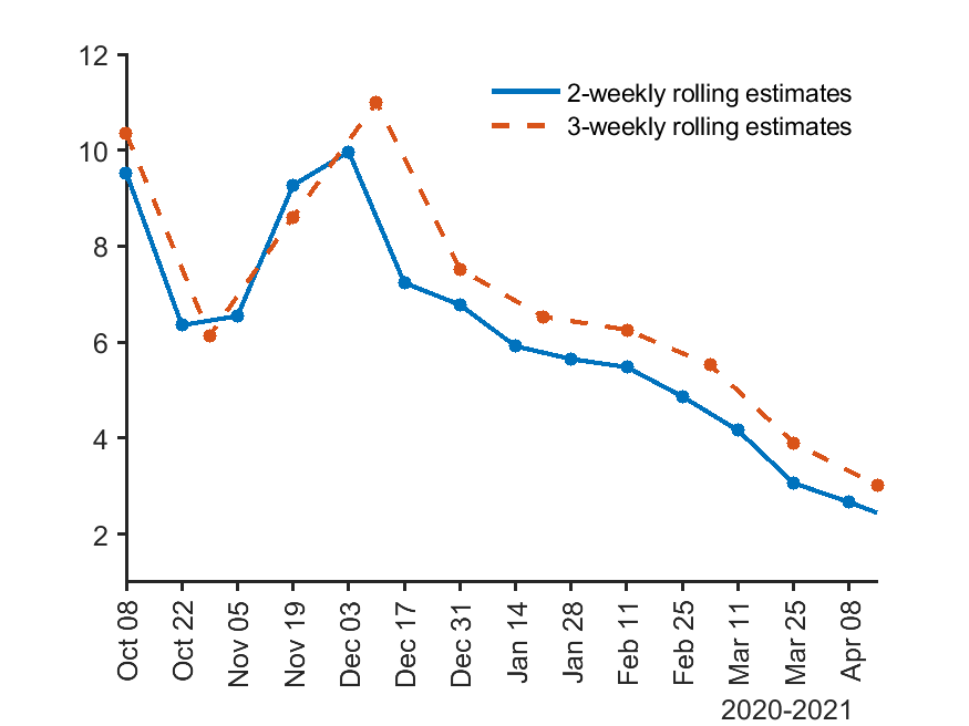
Germany		Italy
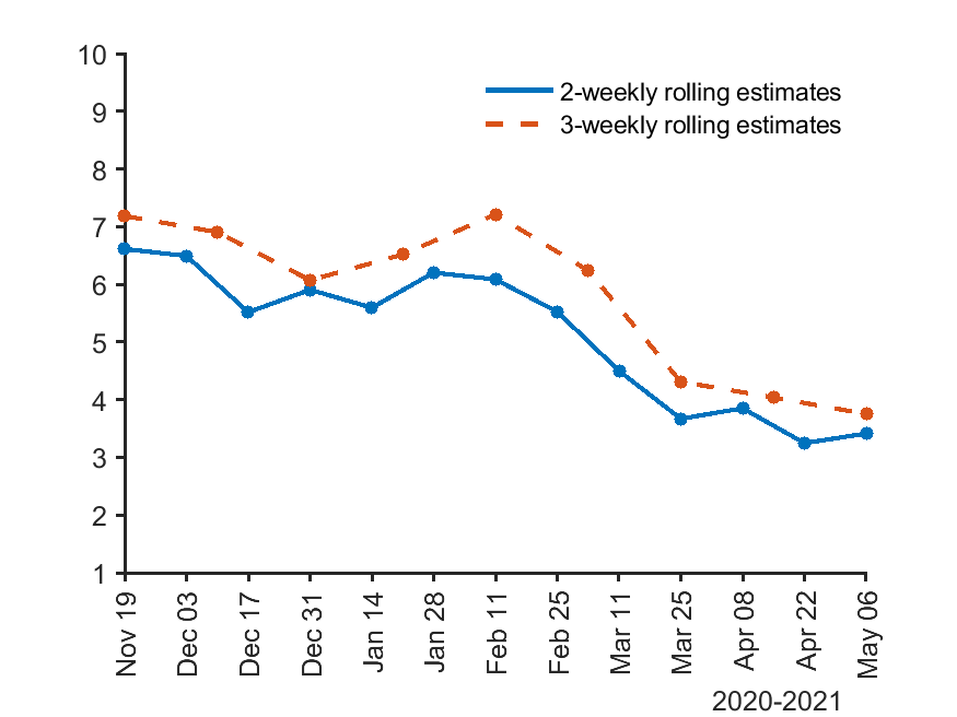
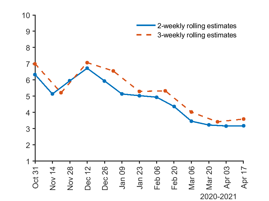
Spain		UK

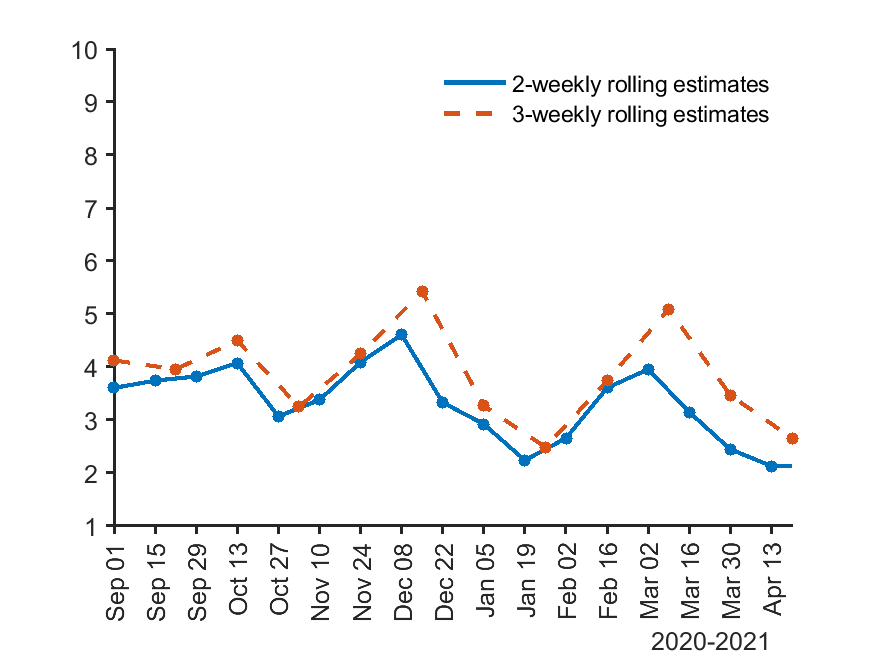
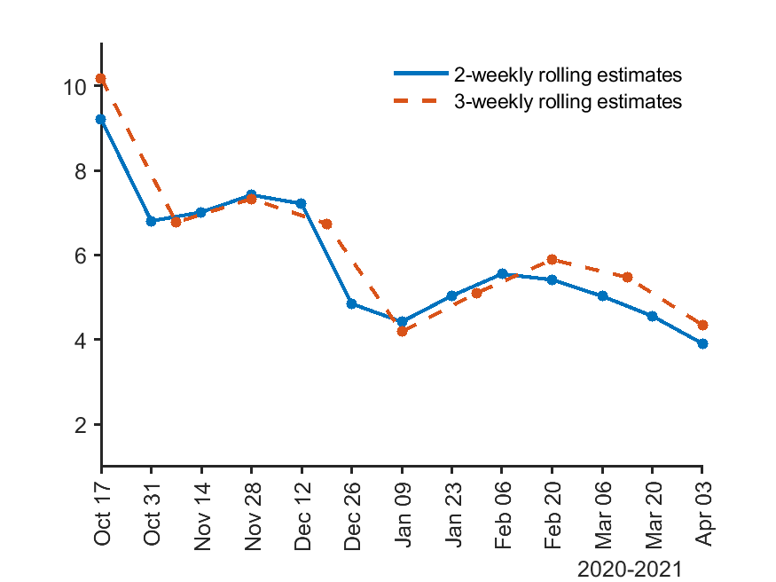
Notes: See the notes to Figure S.7.

It is interesting to compare the reported number of total cases with the case numbers after adjusting for under-reporting using the 2-weekly estimates of the MF, which are displayed in Figure 3 of the main paper. Figure S.11 plots the 7-day moving average of infected cases (per $100,000$ people) for the six countries using the more recent data as of August 5, 2021. The left panel displays the raw data. The right panel shows the MF-adjusted total cases computed by accumulating $\hat{m}_{t}\times\Delta\tilde{c}_{t}$ from the start of the epidemic, where the MF estimates, $\hat{m}_{t}$, was updated every two weeks with values in between obtained by linear interpolation, and $\Delta\tilde{c}_{t}$ is the reported number of daily new cases (per 100k population). The MF is fixed at the last estimate for the period after the joint estimation ends. The figure clearly shows that it is important to adjust the case counts over time by the time-varying MF. We find that, as of August 5, 2021, the number of total cases may be underestimated by three times in Spain, four times in Austria, and five times in the other four countries. After adjusting for under-reporting, we see that Spain ranks fifth in the case rate instead of first. France and the UK have the highest number of cases per capita after adjustment among these countries, approaching $40$ percent in comparison to $8$ percent without adjustment. In contrast, Germany did the best job controlling the total cases even after taking under-reporting into account.

Figure S.11: Total number of infected cases for selected European countries, without and with adjusting for under-reporting

Reported number of cases ($c_{t}$)		$c_{t}$ after adjusting for under-reporting

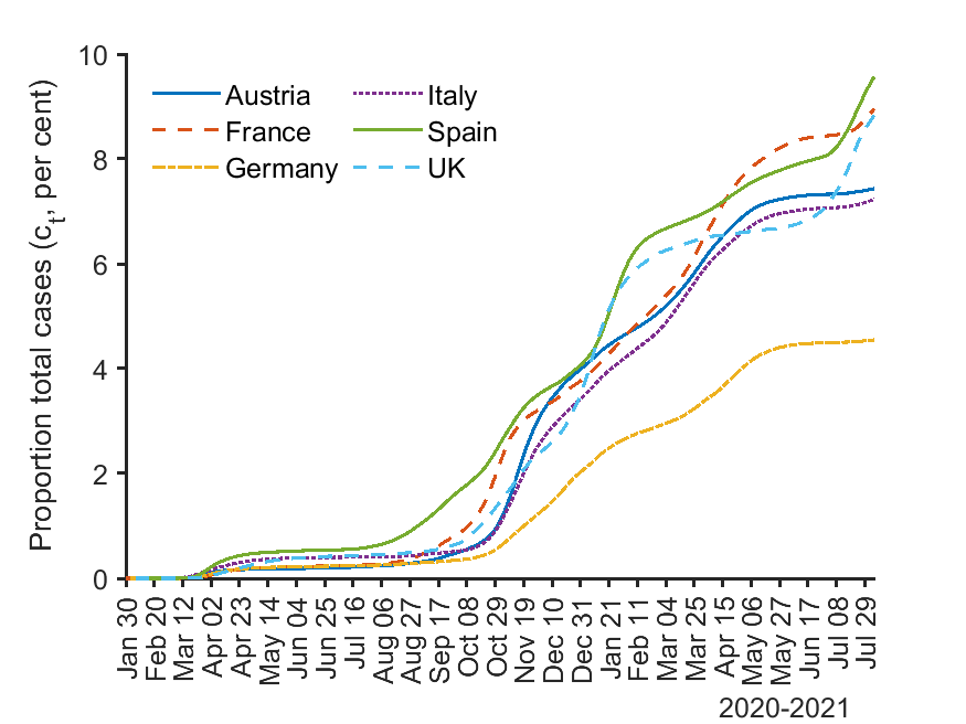
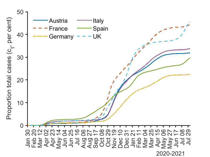
Notes: All series are 7-day moving averages. The figure on the right shows the adjusted number of total cases computed by accumulating $\hat{m}_{t}\times\Delta\tilde{c}_{t}$ from the outbreak to August 5, 2021, where the multiplication factor, $m_{t}$, was updated every two weeks with values in between obtained by linear interpolation.

We next turn to the estimates of MF for the US. The left panel of Figure S.12 presents the 2-weekly estimates of MF obtained by the joint estimation method over the period of March 2020 to March 2021 (when the share of the population fully vaccinated reached $10$ percent). The results show that the estimated MF gradually declined from $7$ to $3$ from July 2020 to March 2021. This finding is in line with an estimate of $7$ times under-reporting by mid-July in the US based on antibody tests (Kalish2021undiagnosed). The right panel of Figure S.12 shows the calibrated new cases compared with the realized cases that have been multiplied by the estimated MF. We can immediately observe that the calibrated cases match the several waves of Covid in the US reasonably well.

Figure S.12: Estimates of the multiplication factor and comparison of realized and calibrated new cases for the US

Estimates of MF		Realized and calibrated new cases

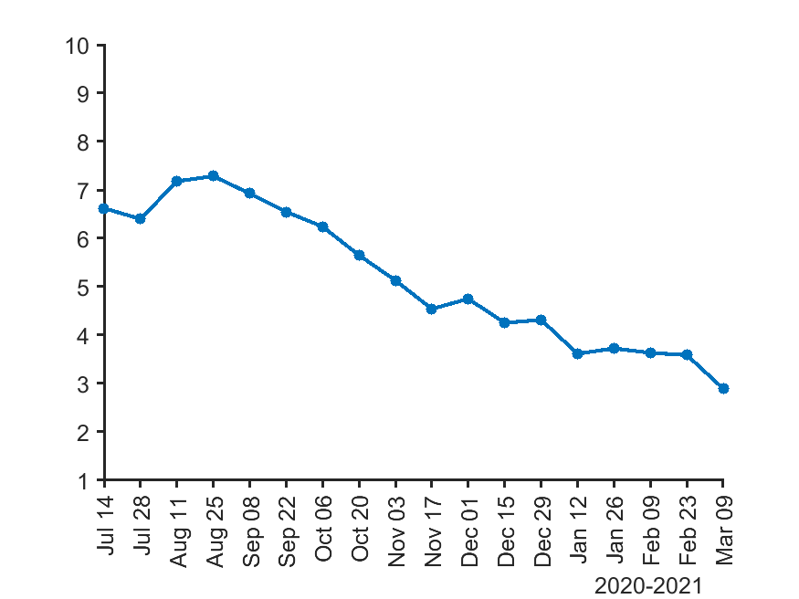
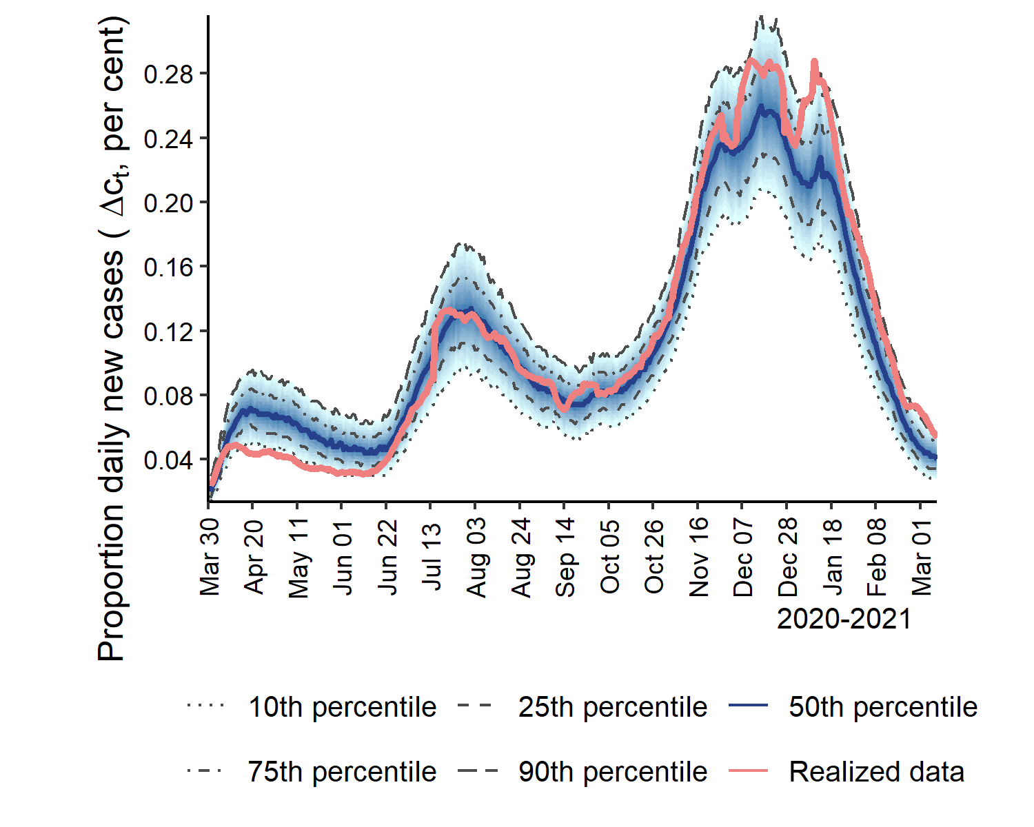
Notes: $\mathcal{\hat{R}}_{et}=\left(1-\hat{m}_{t}\tilde{c}_{t}\right)\hat{\beta}_{t}/\gamma$, where $\tilde{c}_{t}$ is the reported number of infections per capita and $\gamma=1/14.$ $W_{\beta}=W_{m}=2$ weeks. The joint estimation starts when $\tilde{c}_{t}>0.01$. The initial guess estimate of the multiplication factor is $5$. The simulation uses the single group model with population size $n=50,000$. The number of replications is $500$. The number of removed (recoveries + deaths) is estimated recursively using $\tilde{R}_{t}=\left(1-\gamma\right)\tilde{R}_{t-1}+\gamma\tilde{C}_{t-1}$, with $\tilde{C}_{1}=\tilde{R}_{1}=0$. Realized series (7-day moving average) multiplied by the estimated multiplication factor is displayed in red.

Appendix S7 Additional counterfactual exercises

S7.1 Social distancing and vaccination

This section presents the results of additional counterfactual experiments of social distancing and vaccination. We consider the same social distancing policy as described in the main paper: the (scaled) transmission rate, $\beta_{t}/\gamma$, equals $3$ in the first two weeks, falls to $0.9$ linearly over the next three weeks, and remains at $0.9$ for eight weeks. When social distancing is relaxed, the transmission rate increases to $1.5$ linearly over the next three weeks and remains at $1.5$ afterward. Figure S.13 displays the time profile of the transmission rate under this social distancing policy.

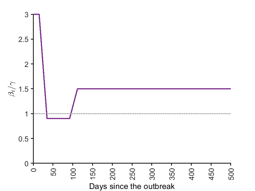
Figure S.13: Time profile of the transmission rate under social distancing

Figure S.14 complements Figure 5 of the main paper and presents additional simulation outcomes under different vaccination coverages, start times, speeds of delivery, and vaccine efficacies under the random vaccination scheme. Specifically, Figure S.14(a) displays the simulated new cases under $50$ and $75$ percent vaccination coverages, which are assumed to take $8$ and $12$ weeks, respectively. The epidemic lasts much longer if the vaccine uptake is lower, although the number of daily new cases and total cases end up very similar. In both cases, the second epidemic wave is successfully prevented. Two important reasons are that the vaccination started early enough (during the last month of social distancing), and the vaccine is highly effective. If the vaccination begins at the end of social distancing (as shown in Figure S.14(b)), there will be a resurgence of cases, resulting in a longer duration of the epidemic and a greater number of total cases. Figure S.14(c) shows that if $75$ percent of the population gets vaccinated over $8$ rather than $12$ weeks, the epidemic could end within $200$ days, and there will not be any uptick in new cases when the social distancing is relaxed. Finally, Figure S.14(d) shows that if the vaccine has $66$ percent efficacy instead of $95$ percent, one would expect to see a small second wave of cases, and the epidemic would last for $65$ days longer.

Figure S.14: Simulated average number of new cases for different random vaccination experiments, with the same social distancing policy

(a) Comparing different vaccination coverages

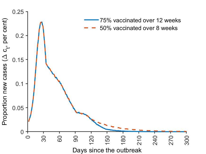
Notes: The average number of new cases over $B=1,000$ replications is displayed. Population size is $n=10,000$. The time profile of $\beta_{t}/\gamma$ under social distancing is displayed in Figure S.13. The vaccination starts during the last month of social distancing (i.e., the $10^{th}$ week after the outbreak). The vaccine efficacy is $\epsilon_{v}=0.95$. If $75$ percent of the population is randomly vaccinated over $12$ weeks, $c^{\ast}=B^{-1}\sum_{b=1}^{B}\max_{t}c_{t}^{(b)}=0.12$, and the duration of the epidemic is $T^{\ast}=215$ days. If $50$ percent of the population is randomly vaccinated over $8$ weeks, $c^{\ast}=0.12$, and $T^{\ast}=270$ days.

(b) Comparing different vaccination start times

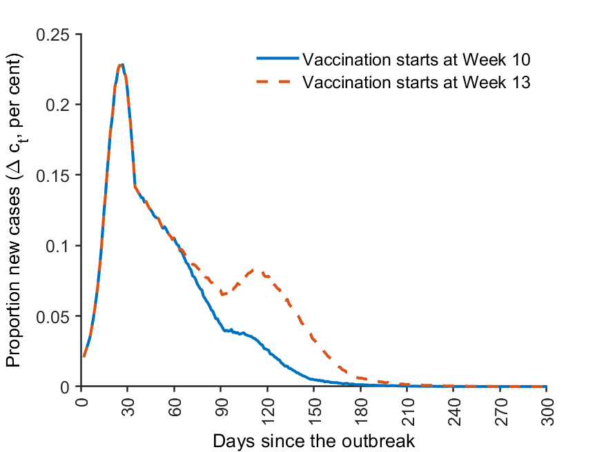
Notes: The average number of new cases over $B=1,000$ replications is displayed. Population size is $n=10,000$. The time profile of $\beta_{t}/\gamma$ under social distancing is displayed in Figure S.13. The vaccine efficacy is $\epsilon_{v}=0.95$. $75$ percent of the population is randomly vaccinated over $12$ weeks. If the vaccination starts during the last month of social distancing (i.e., the $10^{th}$ week after the outbreak), $c^{\ast}=B^{-1}\sum_{b=1}^{B}\max_{t}c_{t}^{(b)}=0.12$, and the duration of the epidemic is $T^{\ast}=215$ days. If the vaccination starts at the end of social distancing (i.e., the $13^{th}$ week after the outbreak), $c^{\ast}=0.15$, and $T^{\ast}=248$ days.

Figure S.14: (Continued) Simulated average number of new cases for different random vaccination experiments, with the same social distancing policy

(c) Comparing different vaccination speeds

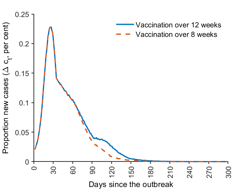
Notes: The average number of new cases over $B=1,000$ replications is displayed. Population size is $n=10,000$. The time profile of $\beta_{t}/\gamma$ under social distancing is displayed in Figure S.13. The vaccination starts during the last month of social distancing (i.e., the $10^{th}$ week after the outbreak). The vaccine efficacy is $\epsilon_{v}=0.95$. $75$ percent of the population is randomly vaccinated. If the vaccination is administered over $12$ weeks, $c^{\ast}=B^{-1}\sum_{b=1}^{B}\max_{t}c_{t}^{(b)}=0.12$, and the duration of the epidemic is $T^{\ast}=215$ days. If the vaccination is administered over $8$ weeks, $c^{\ast}=0.11$, and $T^{\ast}=197$ days.

(d) Comparing different vaccine efficacies

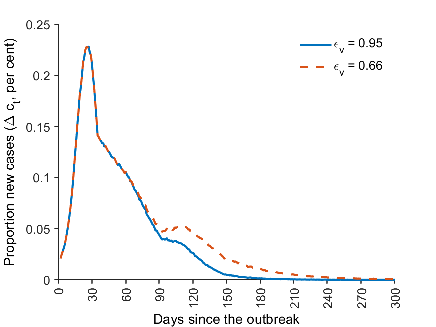
Notes: The average number of new cases over $B=1,000$ replications is displayed. Population size is $n=10,000$. The time profile of $\beta_{t}/\gamma$ under social distancing is displayed in Figure S.13. The vaccination starts during the last month of social distancing (i.e., the $10^{th}$ week after the outbreak). $75$ percent of the population is randomly vaccinated over $12$ weeks. If the vaccine efficacy is $\epsilon_{v}=0.95$, $c^{\ast}=B^{-1}\sum_{b=1}^{B}\max_{t}c_{t}^{(b)}=0.12$, and the duration of the epidemic is $T^{\ast}=215$ days. If $\epsilon_{v}=0.66$, then $c^{\ast}=0.13$, and $T^{\ast}=280$ days.