Analytic estimation of the MMC sub-module capacitor voltage ripple for balanced and unbalanced AC grid conditions

Abstract

In this paper, a mathematical expression to define the maximum and minimum voltage ripples of the modular multilevel converter (MMC) sub-module (SM) capacitors is proposed. Using the arm averaged model of the MMC, the instantaneous power for the upper and lower arms of the converter is obtained, giving the basis to describe the instantaneous energy of the arms. To calculate the SM capacitors peak voltage values, it is required to obtain an analytic expression for the maximum and minimum energy levels. Due to the presence of terms with different magnitudes, frequencies and phases, finding it can be quite challenging. To overcome this issue, the instantaneous arm energy expression is modified using mathematical assumptions in order to join the different components into a single term which can analytically describes the maximum energy point. Then, this expression is used to calculate the peak values of the arm capacitor voltages. By employing the same principles from the arm level, the final analytical expression for the SM capacitors maximum and minimum voltages is found. Simulation results are carried out in order to validate the accuracy of the proposed analysis for different power delivery conditions.

I Introduction

The modular multilevel converter, firstly proposed by [1], is a well-established technology for HVDC transmission systems [2, 3, 4, 5]. Among the main benefits compared to other topologies, the MMC produces high quality output voltage waveforms with low harmonic content, presents reduced transformer $dv/dt$ stress, common DC bus and improved efficiency. Due to these features, the MMC can also be employed in various applications such as medium-voltage motor drives, active filters and microgrids [4].

In microgrids, the MMC can be used in several medium voltage applications [6, 7]. Varying from PV systems [8, 9] to complex interconnection of multiple microgrids [10]. Nevertheless, the MMC sub-modules requires larger capacitance compared to other topologies in order to maintain acceptable voltage ripple levels [11]. In general, the SM capacitor voltage ripple is assumed to be 10% of its mean voltage level [12], but this value can vary according to project requirements. Several authors proposed different studies in order to reduce the SM capacitor voltage fluctuation [13, 14, 15]. However, due to the presence of energy terms with different frequencies, phases and magnitudes, these papers were unable to obtain a concise equation unifying all those elements into a single general expression that can estimate the maximum and minimum energy profiles of the MMC arms.

Having an adequate estimation of the energy ripple can be used during both the design and the operation stages. For instance, during an unbalanced AC voltage sag, the arms of the MMC may present high energy deviations, leading to higher arm capacitor voltages which may exceed the design limitation of the component. Therefore, such expression would be useful to see the impact on the capacitor voltage oscillation when selecting key values of the converter, such as the submodule capacitance. To do so, this paper provides an in-depth mathematical analysis in order to estimate the maximum and minimum submodule capacitor voltages.

Based on the steady-state analysis of the system given in [16], the different arm variables of the MMC can be obtained. Then, they are used to derive the instantaneous upper and lower arm powers that are later integrated and simplified to achieve the final instantaneous energy expression for the converters arms. Afterwards, mathematical manipulations are performed to combine all the terms with different magnitudes, phases and frequencies into a single equation that can calculate the peak values of the arm capacitor voltage in any grid condition. The same considerations employed in the arm level are extended to the SM capacitors; thus, the final equation for the peak SM capacitor voltages can be achieved.

This paper is divided as: Section II describes the converter and its basic equations. Next, in Section III the instantaneous arm power and energy are derived, giving the basis to obtain the maximum and minimum arm capacitor voltages. In Section IV, the analytical mathematical expression for the SM capacitor peak voltages are demonstrated. Section V presents the simulation results to validate the analysis. Finally, the conclusions are given in Section VI.

II System description

The three-phase MMC is a voltage source converter (VSC) consisting of three legs, one per phase, in which each leg has two stacks of $N_{arm}$ half-bridge sub-modules, known as the upper and lower arms. The complexity of the sub-modules can vary according to the application [17].

In Fig. 1, the converter variables are described as follows: $u_{g}^{k}$ is the AC network voltage, $u_{u}^{k}$ and $u_{l}^{k}$ are the upper and lower arms voltages respectively, $U_{u}^{DC}$ and $U_{l}^{DC}$ are the upper and lower DC grid voltages, $i_{u}^{k}$ and $i_{l}^{k}$ are the upper and lower arm currents respectively, $i_{s}^{k}$ is the AC network current, $R_{a}$ and $L_{a}$ are the arm impedances and finally, $R_{s}$ and $L_{s}$ are the phase reactor impedances.

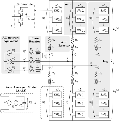
Figure 1: Complete model of the MMC converter.

The mathematical description of the MMC general equations can be obtained per phase $k$ $(\mbox{consider that }k\in\{a,b,c\})$ and is given as,

$$U_{u}^{DC}-u_{u}^{k}-u_{g}^{k}-u_{n}=R_{a}i_{u}^{k}+L_{a}\frac{di_{u}^{k}}{dt}+R_{s}i_{s}^{k}+L_{s}\frac{di_{s}^{k}}{dt}$$ (1)

$$-U_{l}^{DC}+u_{l}^{k}-u_{g}^{k}-u_{n}=-R_{a}i_{l}^{k}-L_{a}\frac{di_{l}^{k}}{dt}+R_{s}i_{s}^{k}+L_{s}\frac{di_{s}^{k}}{dt}$$ (2)

III Derivation of the arm capacitor voltage ripple

The capacitor voltage is highly dependable on the energy flowing through the MMC arms as it can be noted from (3). Under balanced AC network conditions, the arms energy are equitable, resulting in similar voltage profiles for the capacitor ripple. However, during an unbalanced AC voltage sag, the arms of the MMC may present high energy deviations, leading to higher arm capacitor voltages which may exceed the design limitation of the component.

$$E=\dfrac{CU^{2}}{2}$$ (3)

Consequently, the capacitor voltages must be kept within certain limits to ensure a proper operation of the MMC. To find the maximum and minimum ripple of the SM capacitor voltage, the derivation procedure is firstly done for the arm capacitors of the MMC and the same principles are then employed to the SM capacitors.

III-A Instantaneous MMC arm power

Firstly, the instantaneous power for the upper and lower arms are firstly derived in (4a) and (4b) considering that the MMC is operated under steady-state conditions and that the power transfer occurs from the DC side to the AC grid. By doing so, the MMC DC currents are flowing in the same direction as the AC ones.

$$p_{u}^{k}(t)=u_{u}^{k}(t)i_{u}^{k}(t)$$ (4a)

$$p_{l}^{k}(t)=u_{l}^{k}(t)i_{l}^{k}(t)$$ (4b)

By replacing the upper and lower arms voltages and currents by their DC and AC components, respectively, the power equations can be expressed as

$$p_{u}^{k}(t)=\left(U_{u}^{kDC}-\hat{U}_{g}^{k}\cos(\omega t+\theta^{k})\right)\cdot$$

$$\cdot\left(I^{kDC}+\dfrac{\hat{I}_{s}^{k}\cos(\omega t+\delta^{k})}{2}\right)$$ (5a)

$$p_{l}^{k}(t)=\left(U_{l}^{kDC}+\hat{U}_{g}^{k}\cos(\omega t+\theta^{k})\right)\cdot$$

$$\cdot\left(I^{kDC}-\dfrac{\hat{I}_{s}^{k}\cos(\omega t+\delta^{k})}{2}\right)$$ (5b)

with $U_{u,l}^{kDC}$ as the upper and lower arms DC voltages, $I^{kDC}$ as the DC current circulating through the MMC arms, $\delta^{k}$ as the angle between the AC grid voltages and currents and $\theta^{k}$ is the phase-shift between the grid voltage phases. By multiplying the terms in (5a) and (5b), the upper and lower arms power can be expended as follows

$$p_{u}^{k}(t)=U_{u}^{kDC}I^{kDC}+\dfrac{U_{u}^{kDC}\hat{I}_{s}^{k}}{2}\cos(\omega t+\delta^{k})-$$ (6a)

$$-I^{kDC}\hat{U}_{g}^{k}\cos(\omega t+\theta^{k})-\dfrac{\hat{U}_{g}^{k}\hat{I}_{s}^{k}}{2}\cos(\omega t+\theta^{k})\cos(\omega t+\delta^{k})$$

$$p_{l}^{k}(t)=U_{l}^{kDC}I^{kDC}-\dfrac{U_{l}^{kDC}\hat{I}_{s}^{k}}{2}\cos(\omega t+\delta^{k})+$$ (6b)

$$+I^{kDC}\hat{U}_{g}^{k}\cos(\omega t+\theta^{k})-\dfrac{\hat{U}_{g}^{k}\hat{I}_{s}^{k}}{2}\cos(\omega t+\theta^{k})\cos(\omega t+\delta^{k})$$

As it can be observed, the expanded instantaneous power expressions present a term in which two cosines with different phases are multiplied. Using simple trigonometric identities, this term can be simplified as,

$$\dfrac{\hat{U}_{g}^{k}\hat{I}_{s}^{k}}{2}\cos(\omega t+\theta^{k})\cos(\omega t+\delta^{k})=$$ (7)

$$=\dfrac{\hat{U}_{g}^{k}\hat{I}_{s}^{k}}{4}\left[\cos(\theta^{k}-\delta^{k})+\cos(2\omega t+\delta^{k}+\theta^{k})\right]$$

Thus, substituting (7) in (6a) and (6b), the power equations can be rewritten as follows

$$p_{u}^{k}(t)=U_{u}^{kDC}I^{kDC}+\dfrac{U_{u}^{kDC}\hat{I}_{s}^{k}}{2}\cos(\omega t+\delta^{k})-$$ (8a)

$$-I^{kDC}\hat{U}_{g}^{k}\cos(\omega t+\theta^{k})-\dfrac{\hat{U}_{g}^{k}\hat{I}_{s}^{k}}{4}\cos(\theta^{k}-\delta^{k})-$$

$$\qquad\qquad\quad-\dfrac{\hat{U}_{g}^{k}\hat{I}_{s}^{k}}{4}\cos(2\omega t+\delta^{k}+\theta^{k})$$

$$p_{l}^{k}(t)=U_{l}^{kDC}I^{kDC}-\dfrac{U_{l}^{kDC}\hat{I}_{s}^{k}}{2}\cos(\omega t+\delta^{k})+$$ (8b)

$$+I^{kDC}\hat{U}_{g}^{k}\cos(\omega t+\theta^{k})-\dfrac{\hat{U}_{g}^{k}\hat{I}_{s}^{k}}{4}\cos(\theta^{k}-\delta^{k})-$$

$$\qquad\qquad\quad-\dfrac{\hat{U}_{g}^{k}\hat{I}_{s}^{k}}{4}\cos(2\omega t+\delta^{k}+\theta^{k})$$

In steady-state conditions, the AC and DC active power exchanged between the grids should be equal, if the semi-conductor losses are neglected. Obviously, this is not feasible with instantaneous values (as AC power is non-constant). However, it is possible to impose an equality between the AC average power (calculated in the phasor domain) and the DC power, as given in (9). If this condition is not achieved, the energy in the arms cells would either charge or discharge the arm capacitors and therefore, steady-state conditions would not hold.

$$U_{u,l}^{kDC}I^{kDC}=\dfrac{\hat{U}_{g}^{k}\hat{I}_{s}^{k}}{4}\cos(\delta^{k}-\theta^{k})$$ (9)

Based on this, the upper and lower arms powers are reduced to their simplest form,

$$p_{u}^{k}(t)=\dfrac{U_{u}^{kDC}\hat{I}_{s}^{k}}{2}\cos(\omega t+\delta^{k})-I^{kDC}\hat{U}_{g}^{k}\cos(\omega t+\theta^{k})-$$

$$\qquad\qquad\qquad-\dfrac{\hat{U}_{g}^{k}\hat{I}_{s}^{k}}{4}\cos(2\omega t+\delta^{k}+\theta^{k})$$ (10a)

$$p_{l}^{k}(t)=-\dfrac{U_{l}^{kDC}\hat{I}_{s}^{k}}{2}\cos(\omega t+\delta^{k})+I^{kDC}\hat{U}_{g}^{k}\cos(\omega t+\theta^{k})-$$

$$\qquad\qquad\qquad-\dfrac{\hat{U}_{g}^{k}\hat{I}_{s}^{k}}{4}\cos(2\omega t+\delta^{k}+\theta^{k})$$ (10b)

III-B Arms maximum energy and voltage calculation

The capacitor voltage presents the same waveform profile as the arm energy. Therefore, to find the maximum and minimum values of the arm capacitor voltage, it is possible to calculate the peak values of the arm energy. The equation for the instantaneous energy flowing through the MMC arms which can be expressed as

$$\qquad\qquad\qquad\qquad E_{u}^{k}(t)=\int p_{u}^{k}(t)dt$$

$$E_{u}^{k}(t)=\dfrac{U_{u}^{kDC}\hat{I}_{s}^{k}}{2\omega}\sin(\omega t+\delta^{k})-\dfrac{I^{kDC}\hat{U}_{g}^{k}}{\omega}\sin(\omega t+\theta^{k})-$$

$$\qquad\qquad\qquad-\dfrac{\hat{U}_{g}^{k}\hat{I}_{s}^{k}}{8\omega}\sin(2\omega t+\delta^{k}+\theta^{k})$$ (11)

$$\qquad\qquad\qquad\qquad E_{l}^{k}(t)=\int p_{l}^{k}(t)dt$$

$$E_{l}^{k}(t)=-\dfrac{U_{l}^{kDC}\hat{I}_{s}^{k}}{2\omega}\sin(\omega t+\delta^{k})+\dfrac{I^{kDC}\hat{U}_{g}^{k}}{\omega}\sin(\omega t+\theta^{k})-$$

$$\qquad\qquad\qquad-\dfrac{\hat{U}_{g}^{k}\hat{I}_{s}^{k}}{8\omega}\sin(2\omega t+\delta^{k}+\theta^{k})$$ (12)

Even though the expressions for the upper and lower arms instantaneous energy could be obtained through simple mathematical manipulation, finding the maximum value of those can be quite challenging. Such difficult exists due to the presence of terms with different magnitudes, frequencies and phases, as it can be observed in Fig. 2.

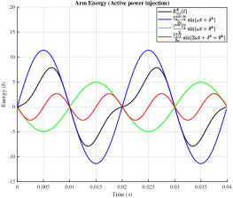
(a) Pure active power injection

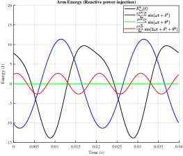
(b) Pure reactive power injection

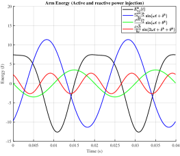
(c) Active and reactive power injection

Figure 2: Energy waveforms for the different energy terms during different power injection conditions.

The energy expression can be simplified by rewriting the terms with same frequency but with different magnitudes and phases as a single equation by employing the following trigonometric identity,

$$\qquad\qquad\qquad A\sin(\omega t+\alpha)+B\sin(\omega t+\beta)=$$

$$=\underbrace{\sqrt{\left[A\cos(\alpha)+B\cos(\beta)\right]^{2}+\left[A\sin(\alpha)+B\sin(\beta)\right]^{2}}}_{\text{X}}\cdot$$

$$\qquad\quad\cdot\sin\left\{\omega t+\underbrace{\tan^{-1}\left[\frac{A\sin(\alpha)+B\sin(\beta)}{A\cos(\alpha)+B\cos(\beta)}\right]}_{\text{$\Psi$}}\right\}$$ (13)

Observing (13), it is clear that the resultant expression represents a vector with maximum magnitude equals to $X$ with a phase of $\Psi$. Therefore, the maximum ripple energy value for the terms at the fundamental frequency can be found by replacing the elements from (11) and (12) in $X$, such as

$$E_{umax_{f}}^{k}=\left(\begin{aligned} \left[\dfrac{U_{u}^{kDC}\hat{I}_{s}^{k}}{2\omega}\cos(\delta^{k})-\dfrac{I^{kDC}\hat{U}_{g}^{k}}{\omega}\cos(\theta^{k})\right]^{2}+\\ +\left[\dfrac{U_{u}^{kDC}\hat{I}_{s}^{k}}{2\omega}\sin(\delta^{k})-\dfrac{I^{kDC}\hat{U}_{g}^{k}}{\omega}\sin(\theta^{k})\right]^{2}\end{aligned}\right)^{1/2}$$ (14)

$$E_{lmax_{f}}^{k}=\left(\begin{aligned} \left[-\dfrac{U_{l}^{kDC}\hat{I}_{s}^{k}}{2\omega}\cos(\delta^{k})+\dfrac{I^{kDC}\hat{U}_{g}^{k}}{\omega}\cos(\theta^{k})\right]^{2}+\\ +\left[-\dfrac{U_{l}^{kDC}\hat{I}_{s}^{k}}{2\omega}\sin(\delta^{k})+\dfrac{I^{kDC}\hat{U}_{g}^{k}}{\omega}\sin(\theta^{k})\right]^{2}\end{aligned}\right)^{1/2}$$ (15)

Therefore the upper and lowers instantaneous energies can be described as,

$$E_{u}^{k}(t)=E_{umax_{f}}^{k}\sin(\omega t+\Psi_{u}^{k})+E_{max_{2f}}^{k}\sin(2\omega t+\delta^{k}+\theta^{k})$$ (16)

$$E_{l}^{k}(t)=E_{lmax_{f}}^{k}\sin(\omega t+\Psi_{l}^{k})+E_{max_{2f}}^{k}\sin(2\omega t+\delta^{k}+\theta^{k})$$ (17)

where, $\Psi_{u}^{k}$ and $\Psi_{l}^{k}$ are the upper and lower phase shifts for phase $k$ obtained using (13) and $E_{max_{2f}}^{k}=\left|-\hat{U}_{g}^{k}\hat{I}_{s}^{k}/8\omega\right|$.

Although the maximum value of the arms energy at the fundamental frequency was obtained, there is still a need to combine them with the second-order components to achieve a general equation that can estimate the maximum energy ripple of the upper and lower arms. Equations (16) and (17) will be maximized when $\sin(\omega t+\Psi_{u,l}^{k})=\sin(2\omega t+\delta^{k}+\theta^{k})=1$; thus,

$$E_{u,lmax}^{kAC}=E_{u,lmax_{f}}^{k}+E_{max_{2f}}^{k}$$ (18)

To comply with the conditions in (18), the angles for the first and second order terms must meet the following condition,

$$\centering\omega t+\Psi_{u,l}^{k}\@add@centering =\pi/2+n_{1}\pi,\text{for }n_{1}\in\mathbb{Z},$$ (19a)

$$2\omega t+\delta^{k}+\theta^{k} =\pi/2+n_{2}\pi,\text{for }n_{2}\in\mathbb{Z}$$ (19b)

$$\pi/2+n_{1}\pi-\Psi_{u,l}^{k} =\left(\pi/2+n_{2}\pi-(\delta^{k}+\theta^{k})\right)/2$$ (19c)

$$\pi+2n_{1}\pi-2\Psi_{u,l}^{k} =\pi/2+n_{2}\pi-(\delta^{k}+\theta^{k})$$ (19d)

$$\pi/2+(2n_{1}-n_{2})\pi =2\Psi_{u,l}^{k}-(\delta^{k}+\theta^{k})$$ (19e)

$$2\Psi_{u,l}^{k}-(\delta^{k}+\theta^{k}) =\pi/2+n\pi$$ (19f)

However, when such condition is not held, the maximum energy level calculated with (18) presents a value deviation. This error is affected by the magnitudes of the energy terms, as well as, the phase displacement between them. In Fig. 3, it can be observed that the maximum energy value ($z$ axis) and, consequently, the minimum error (see (18)) happens when the angles for the second order term sum $90^{o}$ or for high energy ratios, which is in accordance with (19). Whereas, the highest energy deviation occurs when there is no phase shift between $E_{u,lmax_{f}}^{k}$ and $E_{max_{2f}}^{k}$ and small energy ratio, having a value equals to 15%.

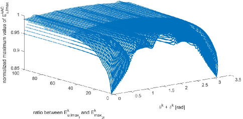
Figure 3: Energy profile for different angle and magnitude values.

As aforementioned, the analysis considers that the MMC is operated in steady-state conditions and, as a result, the capacitors can be considered fully charged. For this reason, they already present an average energy level for the upper and lower arms (20). Moreover, this energy reference must be taken into account when the arm capacitor voltage ripple is calculated.

$$E_{u,l_{ref}}^{k}=\dfrac{C_{SM}}{2N_{arm}}U_{Cu,l_{ref}}^{k^{2}}$$ (20)

where $U_{Cu,l_{ref}}^{k}$ is the arm voltage reference, which is the value of the DC link voltage and $C_{SM}$ is the sub-module capacitance.

Therefore, the maximum and minimum values for the upper and lower arms energy can be mathematically described as

$$E_{u,l_{max,min}}^{k}=\underbrace{E_{u,l_{ref}}^{k}}_{\text{DC term}}\pm\underbrace{E_{u,l_{max}}^{kAC}}_{\text{peak of the AC part}}$$ (21)

By replacing the energy DC term $E_{u,l_{ref}}^{k}$ with the maximum/minimum energy ones $E_{u,l_{max,min}}^{k}$, (21) can be rearranged and the final expression for the peak voltage levels of the MMC arm capacitor can be calculated as,

$$U_{u,l_{max}}^{k}=\sqrt{\dfrac{2E_{u,l_{max}}^{k}N_{arm}}{C_{SM}}}$$ (22)

$$U_{u,l_{min}}^{k}=\sqrt{\dfrac{2E_{u,l_{min}}^{k}N_{arm}}{C_{SM}}}$$ (23)

IV SM capacitor maximum and minimum voltages

Until now, the derivation procedure was done in the arm level. However, as aforementioned, the main goal is to obtain a mathematical expression for the maximum and minimum voltages of the individual SM capacitors of the MMC. Based on the arm expressions, the same principles are used for the SM capacitors and the final general expression for their peak voltages can be calculated. Again, it is considered that the MMC is operated under steady-state conditions to ensure that all the SM capacitors are fully charged.

The first step is to modify the upper and lower arms energy expressions given in (11) and (12) into equations that can describe the energy profile in the SM level. This can be easily done by dividing those expression by the number of SM per arm, as

$$\qquad\qquad\qquad\qquad E_{u}^{k}(t)=\int p_{u}^{k}(t)dt$$

$$E_{SMu}^{k}(t)=\dfrac{U_{u}^{kDC}\hat{I}_{s}^{k}}{2\omega N_{arm}}\sin(\omega t+\delta^{k})-\dfrac{I^{kDC}\hat{U}_{g}^{k}}{\omega N_{arm}}\sin(\omega t+\theta^{k})-$$

$$\qquad\qquad\qquad-\dfrac{\hat{U}_{g}^{k}\hat{I}_{s}^{k}}{8\omega N_{arm}}\sin(2\omega t+\delta^{k}+\theta^{k})$$ (24)

$$\qquad\qquad\qquad\qquad E_{l}^{k}(t)=\int p_{l}^{k}(t)dt$$

$$E_{SMl}^{k}(t)=-\dfrac{U_{l}^{kDC}\hat{I}_{s}^{k}}{2\omega N_{arm}}\sin(\omega t+\delta^{k})+\dfrac{I^{kDC}\hat{U}_{g}^{k}}{\omega N_{arm}}\sin(\omega t+\theta^{k})-$$

$$\qquad\qquad\qquad-\dfrac{\hat{U}_{g}^{k}\hat{I}_{s}^{k}}{8\omega N_{arm}}\sin(2\omega t+\delta^{k}+\theta^{k})$$ (25)

Then, employing similar procedures used to obtain the maximum energy for the upper and lower arms (18) the maximum SM energy levels can be expressed as follows

$$\centering E_{SMu_{max}}^{kAC}\@add@centering =E_{SM_{umax_{f}}}^{k}+E_{SM_{umax_{2f}}}^{k}$$ (26a)

$$E_{SMu_{max}}^{kAC} =\dfrac{E_{umax}^{kAC}}{N_{arm}}$$ (26b)

$$E_{SMl_{max}}^{kAC} =E_{SM_{lmax_{f}}}^{k}+E_{SM_{lmax_{2f}}}^{k}$$ (27a)

$$E_{SMl_{max}}^{kAC} =\dfrac{E_{lmax}^{kAC}}{N_{arm}}$$ (27b)

The DC energy levels for SM capacitors can be described modifying (20) as

$$E_{SM{u,l_{ref}}}^{k}=\dfrac{C_{SM}}{2}U_{SM}^{2}$$ (28)

where $U_{SM}$ is the average SM capacitor voltage.

Analogously to the maximum and minimum arm energies (21), the peak energy values for the SM capacitors can be calculated as,

$$E_{SMu,l_{max,min}}^{k}=E_{SM{u,l_{ref}}}^{k}\pm E_{SMu,l_{max}}^{kAC}$$ (29)

Finally, the analytic expressions to described the maximum and minimum voltages for the SM capacitors are obtained removing the number of SM in (22) and (23), resulting in

$$U_{Cu,l_{max}}^{k}=\sqrt{\dfrac{2E_{SMu,l_{max}}^{k}}{C_{SM}}}$$ (30)

$$U_{Cu,l_{min}}^{k}=\sqrt{\dfrac{2E_{SMu,l_{min}}^{k}}{C_{SM}}}$$ (31)

V Results

In this section, the proposed analytical expressions to calculate the peak values of the SM capacitor voltages are compared with the maximum and minimum levels obtained using the full energy expressions given in (24) and (25). Firstly, the MMC phase variables were determined through the steady-state analysis developed in [16] using the parameters presented in Table I, which corresponds to an application where the MMC was used as the interface between the main AC distributed grid with different local AC and DC networks. Based on those values, the energy for the SM capacitors were obtained and used to calculate the peak values of the SM capacitor voltages.

In order to validate the proposed mathematical analysis, the converter was considered to be operated in all four different quadrants. Moreover, the different power transfer conditions were analyzed based on balanced AC and DC grid conditions and the displayed quantities are related to phase $a$.

TABLE I: System parameters

Parameter	Symbol	Value	Units
Rated power	$S$	10	kVA
AC-side voltage	$U_{g}$	400	V rms ph-ph
DC link voltage	$U^{DC}$	$\pm$350	V
Phase reactor impedance	$Z_{s}$	j0.24	$\Omega$
Arm reactor impedance	$Z_{a}$	j1.57	$\Omega$
Converter modules per arm	$N_{arm}$	8	-
Average module voltage	$U_{SM}$	87.5	V
Sub-module capacitance	$C_{SM}$	1	mF

In Table II, the maximum and minimum SM capacitor voltages are shown when the values are obtained using the full energy expression and using the proposed peak energy equation. Whereas, in Table III the values for the fundamental and second order frequencies energy terms, as well as, their respective phases are given for the proposed analysis. Finally, the errors for the different power delivery scenarios are displayed in Table IV.

Observing Table III, it can be noted that the value of the second-order energy term is practically constant for different scenarios, since the RMS levels for the grid current and voltage are the same for all the cases. On the other hand, the other quantities changed depending on the power transfer condition as the DC terms and phases have to change in order to absorb or inject reactive power.

The negative signal in the errors for the maximum SM capacitor voltage indicates that the values obtained by the proposed analysis were smaller than the actual level, which can be considered a safety factor during the design stage. Meanwhile, the positive signal in the errors for the minimum voltages implies that the estimated magnitudes are also lower than the real ones. Contrarily to the maximum voltage case, the prediction of lower minimum voltages is undesirable since it can affect the normal operation of the MMC depending to the circumstances. Therefore, in cases where the converter is required to inject reactive power to the AC grid, the addition of a factor of safety to reduce the error, is recommended, and it can be assessed using Fig. 3.

The values obtained in Tables IV are in agreement with the proposed analysis. The two scenarios where the errors are equal to zero are the same as predicted in (19). For the other power delivery conditions, the error profile respects the ones observed in Fig. 3.

TABLE II: Results (Part I)

Power references	Full equation [V]		Proposed method [V]
[kW]	Maximum	Minimum	Maximum	Minimum
P = 10, Q = 0	98.410	75.823	99.644	73.372
P = 7.07, Q = 7.07	97.415	68.788	103.25	68.205
P = 0, Q = 10	99.175	64.424	105.65	64.424
P = -7.07, Q = 7.07	97.415	68.788	103.250	68.205
P = -10, Q = 0	98.410	75.823	99.6445	73.3732
P = -7.07, Q = -7.07	103.24	76.47	102.917	68.7067
P = 0, Q = -10	105.65	74.005	105.65	64.424
P = 7.07, Q = -7.07	103.24	76.47	102.917	68.707

TABLE III: Results (Part II)

$E_{SM_{umax_{f}}}^{a}$ [J]	$E_{SM_{umax_{2f}}}^{a}$ [J]	$\Psi^{a}$ [rad]	($\theta^{a}+\delta^{a}$) [rad]
0.8047	0.3316	-0.0490	0.0637
1.1707	0.3315	-1.0644	-0.7423
1.4213	0.3316	1.5708	-1.5708
1.1707	0.3315	1.0644	-2.3993
0.8047	0.3316	0.0490	-3.2053
1.1363	0.3315	-1.0475	2.3090
1.4213	0.3316	1.5708	1.5708
1.1363	0.3315	1.0475	0.8326

TABLE IV: Error between the values from the full equation and the suggested analysis

Power references	Error [%]
[kW]	Maximum	Minimum
P = 10, Q = 0	-1.253	3.231
P = 7.07, Q = 7.07	-5.990	0.848
P = 0, Q = 10	-6.529	0
P = -7.07, Q = 7.07	-5.99	0.848
P = -10, Q = 0	-1.253	3.231
P = -7.07, Q = -7.07	0.3125	10.15
P = 0, Q = -10	0	12.946
P = 7.07, Q = -7.07	0.313	10.152

VI Conclusions

In this paper, the MMC sub-module capacitors voltage was analyzed and a mathematical estimation of their maximum and minimum voltages was proposed. By considering the arm averaged model, the instantaneous power and energy arm equations were derived. Using mathematical assumptions, the terms with different magnitudes, frequencies and phases were transformed into a single equation which could describe the peak values of the arm capacitor energy ripple for different scenarios.

In steady-state conditions, the arm capacitors can be considered fully charged, consequently, they present a DC energy term that was added with the energy ripple. Then, the summed expression was used to calculate the maximum and minimum voltage ripples of the arm capacitor. Based on the process used for arm capacitors, the SM capacitor instantaneous energy was derived. Furthermore, similar procedures were employed to simplify the SM capacitor energy, allowing the final expression for the SM capacitor peak voltages to be calculated.

Simulation results were carried out to validate the proposed analysis for different power delivery conditions. The results have showed that the SM capacitor voltage ripples were in agreement with the profiles established during the derivation procedures. Finally, the analysis developed by this paper can be employed in future works in order to improve the current reference calculation techniques which may include capacitor voltage limitation issues in any grid voltage condition.

VII Acknowledgments

This project has received funding from the European Union’s Horizon 2020 research and innovation programme under the Marie Sklodowska-Curie grant agreement no. 765585. This document reflects only the author’s views; the European Commission is not responsible for any use that may be made of the information it contains. This work was partially supported by the Spanish Ministry of Science, Innovation and Universities under the Project RTI2018-095429-B-I00. This work was co-financed by the European Regional Development Fund. E. Prieto is lecturer of the Serra Húnter Programme.

References

- [1] A. Lesnicar and R. Marquardt, “An innovative modular multilevel converter topology suitable for a wide power range,” in 2003 IEEE Bologna Power Tech Conference Proceedings,, vol. 3, June 2003, p. 6 pp. Vol.3.
- [2] D. Van Hertem, O. Gomis-Bellmunt, and J. Liang, HVDC Grids: For Offshore and Supergrid of the Future, ser. IEEE Press Series on Power Engineering. Wiley, 2016.
- [3] E. Prieto-Araujo, A. Junyent-Ferré, G. Clariana-Colet, and O. Gomis-Bellmunt, “Control of modular multilevel converters under singular unbalanced voltage conditions with equal positive and negative sequence components,” IEEE Transactions on Power Systems, vol. 32, no. 3, pp. 2131–2141, May 2017.
- [4] A. Dekka, B. Wu, R. L. Fuentes, M. Perez, and N. R. Zargari, “Evolution of topologies, modeling, control schemes, and applications of modular multilevel converters,” IEEE Journal of Emerging and Selected Topics in Power Electronics, vol. 5, no. 4, pp. 1631–1656, Dec 2017.
- [5] E. Sánchez-Sánchez, E. Prieto-Araujo, A. Junyent-Ferré, and O. Gomis-Bellmunt, “Analysis of mmc energy-based control structures for vsc-hvdc links,” IEEE Journal of Emerging and Selected Topics in Power Electronics, vol. 6, no. 3, pp. 1065–1076, Sep. 2018.
- [6] A. Lachichi, A. Junyent-Ferre, and T. C. Green, “Comparative optimization design of a modular multilevel converter tapping cells and a 2l-vsc for hybrid lv ac/dc microgrids,” IEEE Transactions on Industry Applications, vol. 55, no. 3, pp. 3228–3240, May 2019.
- [7] A. Sallam, M. E. Nassar, R. A. R. Hamdy, and M. M. A. Salama, “Interlinked hybrid microgrids with fault confining capability using a novel mmc topology,” in 2017 IEEE Electrical Power and Energy Conference (EPEC), Oct 2017, pp. 1–5.
- [8] J. S. Artal-Sevil, J. A. Domínguez-Navarro, I. Sanz-Gorrachategui, and A. Coronado-Mendoza, “Control strategy for modular multilevel converter applied to active power injection and reactive power compensation: Integration in pv microgrids.” in 2019 Fourteenth International Conference on Ecological Vehicles and Renewable Energies (EVER), May 2019, pp. 1–11.
- [9] M. S. Shadlu, “A comparative study between two mppt algorithms for photovoltaic energy conversion system based on modular multilevel converter,” in Electrical Engineering (ICEE), Iranian Conference on, May 2018, pp. 1154–1159.
- [10] P. Wu, W. Huang, and N. Tai, “Advanced design of microgrid interface for multiple microgrids based on mmc and energy storage unit,” The Journal of Engineering, vol. 2017, no. 13, pp. 2231–2235, 2017.
- [11] S. Yang, J. Fang, Y. Tang, H. Qiu, C. Dong, and P. Wang, “Modular multilevel converter synthetic inertia-based frequency support for medium-voltage microgrids,” IEEE Transactions on Industrial Electronics, vol. 66, no. 11, pp. 8992–9002, Nov 2019.
- [12] L. Harnefors, A. Antonopoulos, S. Norrga, L. Angquist, and H. Nee, “Dynamic analysis of modular multilevel converters,” IEEE Transactions on Industrial Electronics, vol. 60, no. 7, pp. 2526–2537, July 2013.
- [13] M. Vasiladiotis, N. Cherix, and A. Rufer, “Accurate capacitor voltage ripple estimation and current control considerations for grid-connected modular multilevel converters,” IEEE Transactions on Power Electronics, vol. 29, no. 9, pp. 4568–4579, Sep. 2014.
- [14] B. Li, Y. Zhang, G. Wang, W. Sun, D. Xu, and W. Wang, “A modified modular multilevel converter with reduced capacitor voltage fluctuation,” IEEE Transactions on Industrial Electronics, vol. 62, no. 10, pp. 6108–6119, Oct 2015.
- [15] S. Sau and B. G. Fernandes, “Modular multilevel converter based variable speed drive with reduced capacitor ripple voltage,” IEEE Transactions on Industrial Electronics, vol. 66, no. 5, pp. 3412–3421, May 2019.
- [16] D. W. Spier, O. G. Bellmunt, E. P. Araujo, and J. L. Mestre, “Steady-state analysis of the modular multilevel converter,” in Accepted for the IEEE Annual Conference of the Industrial Electronics Society, October 2019, pp. 1–6.
- [17] K. Sharifabadi, L. Harnefors, H. P. Nee, S. Norrga, and R. Teodorescu, Design, Control and Application of Modular Multilevel Converters for HVDC Transmission Systems. Wiley-IEEE press, 2016.