$\infty$-former: Infinite Memory Transformer

Abstract

Transformers are unable to model long-term memories effectively, since the amount of computation they need to perform grows with the context length. While variations of efficient transformers have been proposed, they all have a finite memory capacity and are forced to drop old information. In this paper, we propose the $\infty$-former, which extends the vanilla transformer with an unbounded long-term memory. By making use of a continuous-space attention mechanism to attend over the long-term memory, the $\infty$-former’s attention complexity becomes independent of the context length, trading off memory length with precision. In order to control where precision is more important, $\infty$-former maintains “sticky memories,” being able to model arbitrarily long contexts while keeping the computation budget fixed. Experiments on a synthetic sorting task, language modeling, and document grounded dialogue generation demonstrate the $\infty$-former’s ability to retain information from long sequences.

1 Introduction

When reading or writing a document, it is important to keep in memory the information previously read or written. Humans have a remarkable ability to remember long-term context, keeping in memory the relevant details (Carroll, 2007; Kuhbandner, 2020). Recently, transformer-based language models have achieved impressive results by increasing the context size Radford et al. (2018, 2019); Dai et al. (2019); Rae et al. (2019); Brown et al. (2020). However, while humans process information sequentially, updating their memories continuously, and recurrent neural networks (RNNs) update a single memory vector during time, transformers do not – they exhaustively query every representation associated to the past events. Thus, the amount of computation they need to perform grows with the length of the context, and, consequently, transformers have computational limitations about how much information can fit into memory. For example, a vanilla transformer requires quadratic time to process an input sequence and linear time to attend to the context when generating every new word.

Several variations have been proposed to address this problem (Tay et al., 2020b). Some propose using sparse attention mechanisms, either with data-dependent patterns (Kitaev et al., 2020; Vyas et al., 2020; Tay et al., 2020a; Roy et al., 2021; Wang et al., 2021) or data-independent patterns (Child et al., 2019; Beltagy et al., 2020; Zaheer et al., 2020), reducing the self-attention complexity (Katharopoulos et al., 2020; Choromanski et al., 2021; Peng et al., 2021; Jaegle et al., 2021), and caching past representations in a memory (Dai et al., 2019; Rae et al., 2019). These models are able to reduce the attention complexity, and, consequently, to scale up to longer contexts. However, as their complexity still depends on the context length, they cannot deal with unbounded context.

In this paper, we propose the $\infty$-former (infinite former; Fig. 1): a transformer model extended with an unbounded long-term memory (LTM), which allows the model to attend to arbitrarily long contexts. The key for making the LTM unbounded is a continuous-space attention framework (Martins et al., 2020) which trades off the number of information units that fit into memory (basis functions) with the granularity of their representations. In this framework, the input sequence is represented as a continuous signal, expressed as a linear combination of $N$ radial basis functions (RBFs). By doing this, the $\infty$-former’s attention complexity is ${\mathcal{O}(L^{2}+L\times N)}$ while the vanilla transformer’s is $\mathcal{O}(L\times(L+L_{\mathrm{LTM}}))$, where $L$ and $L_{\mathrm{LTM}}$ correspond to the transformer input size and the long-term memory length, respectively (details in §3.1.1). Thus, this representation comes with two significant advantages: (i) the context can be represented using a number of basis functions $N$ smaller than the number of tokens, reducing the attention computational cost; and (ii) $N$ can be fixed, making it possible to represent unbounded context in memory, as described in §3.2 and Fig. 2, without increasing its attention complexity. The price, of course, is a loss in resolution: using a smaller number of basis functions leads to lower precision when representing the input sequence as a continuous signal, as shown in Fig. 3.

To mitigate the problem of losing resolution, we introduce the concept of “sticky memories” (§3.3), in which we attribute a larger space in the LTM’s signal to regions of the memory more frequently accessed. This creates a notion of “permanence” in the LTM, allowing the model to better capture long contexts without losing the relevant information, which takes inspiration from long-term potentiation and plasticity in the brain (Mills et al., 2014; Bamji, 2005).

To sum up, our contributions are the following:

• We propose the $\infty$-former, in which we extend the transformer model with a continuous long-term memory (§3.1). Since the attention computational complexity is independent of the context length, the $\infty$-former is able to model long contexts.

• We propose a procedure that allows the model to keep unbounded context in memory (§3.2).

• We introduce sticky memories, a procedure that enforces the persistence of important information in the LTM (§3.3).

• We perform empirical comparisons in a synthetic task (§4.1), which considers increasingly long sequences, in language modeling (§4.2), and in document grounded dialogue generation (§4.3). These experiments show the benefits of using an unbounded memory.

2 Background

2.1 Transformer

A transformer Vaswani et al. (2017) is composed of several layers, which encompass a multi-head self-attention layer followed by a feed-forward layer, along with residual connections He et al. (2016) and layer normalization Ba et al. (2016).

Let us denote the input sequence as ${X=[x_{1},\dots,x_{L}]\in\mathbb{R}^{L\times e}}$, where $L$ is the input size and $e$ is the embedding size of the attention layer. The queries $Q$, keys $K$, and values $V$, to be used in the multi-head self-attention computation are obtained by linearly projecting the input, or the output of the previous layer, $X$, for each attention head $h$:

$$\!\!\!Q_{h}=X_{h}W^{Q_{h}},\;K_{h}=X_{h}W^{K_{h}},\; V_{h}=X_{h}W^{V_{h}},\!$$ (1)

where ${W^{Q_{h}},W^{K_{h}},W^{V_{h}}\in\mathbb{R}^{d\times d}}$ are learnable projection matrices, $d=\nicefrac{{e}}{{H}}$, and $H$ is the number of heads. Then, the context representation ${Z_{h}\in\mathbb{R}^{L\times d}}$, that corresponds to each attention head $h$, is obtained as:

$$Z_{h}=\operatorname*{\mathsf{softmax}}\left(\dfrac{Q_{h}K_{h}^{\top}}{\sqrt{d}}\right)V_{h},$$ (2)

where the softmax is performed row-wise. The head context representations are concatenated to obtain the final context representation ${Z\in\mathbb{R}^{L\times e}}$:

$$Z=[Z_{1},\dots,Z_{H}]W^{R},$$ (3)

where ${W^{R}\in\mathbb{R}^{e\times e}}$ is another projection matrix that aggregates all head’s representations.

2.2 Continuous Attention

Continuous attention mechanisms (Martins et al., 2020) have been proposed to handle arbitrary continuous signals, where the attention probability mass function over words is replaced by a probability density over a signal. This allows time intervals or compact segments to be selected.

To perform continuous attention, the first step is to transform the discrete text sequence represented by ${X\in\mathbb{R}^{L\times e}}$ into a continuous signal. This is done by expressing it as a linear combination of basis functions. To do so, each $x_{i}$, with ${i\in\{1,\dots,L\}}$, is first associated with a position in an interval, ${t_{i}\in[0,1]}$, e.g., by setting $t_{i}=i/L$. Then, we obtain a continuous-space representation ${\bar{X}(t)\in\mathbb{R}^{e}}$, for any $t\in[0,1]$ as:

$$\bar{X}(t)=B^{\top}\psi(t),$$ (4)

where ${\psi(t)\in\mathbb{R}^{N}}$ is a vector of $N$ RBFs, e.g., $\psi_{j}(t)=\mathcal{N}(t;\mu_{j},\sigma_{j})$, with $\mu_{j}\in[0,1]$, and ${B\in\mathbb{R}^{N\times e}}$ is a coefficient matrix. $B$ is obtained with multivariate ridge regression (Brown et al., 1980) so that ${\bar{X}(t_{i})\approx x_{i}}$ for each $i\in[L]$, which leads to the closed form (see App. A for details):

$$B^{\top}=X^{\top}F^{\top}(FF^{\top}+\lambda I)^{-1}=X^{\top}G,$$ (5)

where ${F=[\psi(t_{1}),\dots,\psi(t_{L})]\in\mathbb{R}^{N\times L}}$ packs the basis vectors for the $L$ locations. As ${G\in\mathbb{R}^{L\times N}}$ only depends of $F$, it can be computed offline.

Having converted the input sequence into a continuous signal $\bar{X}(t)$, the second step is to attend over this signal. To do so, instead of having a discrete probability distribution over the input sequence as in standard attention mechanisms (like in Eq. 2), we have a probability density $p$, which can be a Gaussian ${\mathcal{N}(t;\mu,\sigma^{2})}$, where $\mu$ and $\sigma^{2}$ are computed by a neural component. A unimodal Gaussian distribution encourages each attention head to attend to a single region, as opposed to scattering its attention through many places, and enables tractable computation. Finally, having $p$, we can compute the context vector $c$ as:

$$c=\mathbb{E}_{p}\left[\bar{X}(t)\right].$$ (6)

Martins et al. (2020) introduced the continuous attention framework for RNNs. In the following section (§3.1), we will explain how it can be used for transformer multi-head attention.

3 Infinite Memory Transformer

To allow the model to access long-range context, we propose extending the vanilla transformer with a continuous LTM, which stores the input embeddings and hidden states of the previous steps. We also consider the possibility of having two memories: the LTM and a short-term memory (STM), which consists in an extension of the transformer’s hidden states and is attended to by the transformer’s self-attention, as in the transformer-XL (Dai et al., 2019). A diagram of the model is shown in Fig. 1.

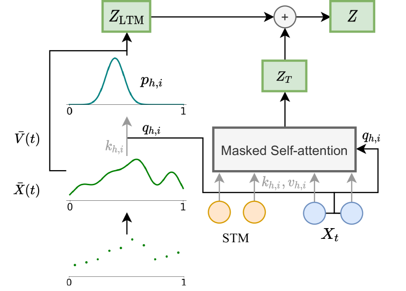
Figure 1: $\infty$-former’s attention diagram with sequence of text, $X_{t}$, of size $L=2$ and STM of size $L_{\mathrm{STM}}=2$. Circles represent input embeddings or hidden states (depending on the layer) for head $h$ and query $i$. Both the self-attention and the attention over the LTM are performed in parallel for each head and query.

3.1 Long-term Memory

For simplicity, let us first assume that the long-term memory contains an explicit input discrete sequence $X$ that consists of the past text sequence’s input embeddings or hidden states, depending on the layer (we will later extend this idea to an unbounded memory in §3.2).

First, we need to transform $X$ into a continuous approximation $\bar{X}(t)$. We compute $\bar{X}(t)$ as:

$$\bar{X}(t)=B^{\top}\psi(t),$$ (7)

where ${\psi(t)\in\mathbb{R}^{N}}$ are basis functions and coefficients ${B\in\mathbb{R}^{N\times e}}$ are computed as in Eq. 5, $B^{\top}=X^{\top}G$. Then, we can compute the LTM keys, ${K_{h}\in\mathbb{R}^{N\times d}}$, and values, ${V_{h}\in\mathbb{R}^{N\times d}}$, for each attention head $h$, as:

$$K_{h}=B_{h}W^{K_{h}},\;\;\;V_{h}=B_{h}W^{V_{h}},$$ (8)

where ${W^{K_{h}},W^{V_{h}}\in\mathbb{R}^{d\times d}}$ are learnable projection matrices. For each query ${q_{h,i}\text{ for }i\in\{1,\dots,L\}}$, we use a parameterized network, which takes as input the attention scores, to compute ${\mu_{h,i}\in]0,1[}$ and ${\sigma_{h,i}^{2}\in\mathbb{R}_{>0}}$:

$$\mu_{h,i}\! =\!\mathrm{sigmoid}\left(\mathrm{affine}\left(\frac{K_{h}\;q_{h,i}}{\sqrt{d}}\right)\right)$$ (9)

$$\sigma^{2}_{h,i}\! =\!\mathrm{softplus}\left(\mathrm{affine}\left(\frac{K_{h}\;q_{h,i}}{\sqrt{d}}\right)\right).$$ (10)

Then, using the continuous softmax transformation (Martins et al., 2020), we obtain the probability density $p_{h,i}$ as ${\mathcal{N}(t;\mu_{h,i},\sigma_{h,i}^{2})}$.

Finally, having the value function $\bar{V}_{h}(t)$ given as ${\bar{V}_{h}(t)=V_{h}^{\top}\psi(t),}$ we compute the head-specific representation vectors as in Eq. 6:

$$z_{h,i}=\mathbb{E}_{p_{h,i}}[\bar{V}_{h}]=V_{h}^{\top}\mathbb{E}_{p_{h,i}}[\psi(t)]$$ (11)

which form the rows of matrix ${Z_{{\mathrm{LTM}},h}\in\mathbb{R}^{L\times d}}$ that goes through an affine transformation, ${Z_{\mathrm{LTM}}=[Z_{{\mathrm{LTM}},1},\dots,Z_{{\mathrm{LTM}},{H}}]W^{O}}$.

The long-term representation, $Z_{\mathrm{LTM}}$, is then summed to the transformer context vector, $Z_{\mathrm{T}}$ , to obtain the final context representation ${Z\in\mathbb{R}^{L\times e}}$:

$$Z=Z_{\mathrm{T}}+Z_{\mathrm{LTM}},$$ (12)

which will be the input to the feed-forward layer.

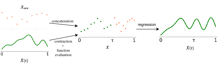
Figure 2: Diagram of the unbounded memory update procedure. This is performed in parallel for each embedding dimension, and repeated throughout the input sequence. We propose two alternatives to select the positions used for the function evaluation: linearly spaced or sticky memories.

3.1.1 Attention Complexity

As the $\infty$-former makes use of a continuous-space attention framework (Martins et al., 2020) to attend over the LTM signal, its key matrix size ${K_{h}\in\mathbb{R}^{N\times d}}$ depends only on the number of basis functions $N$, but not on the length of the context being attended to. Thus, the $\infty$-former’s attention complexity is also independent of the context’s length. It corresponds to ${\mathcal{O}(L\times(L+L_{\mathrm{STM}})+L\times N)}$ when also using a short-term memory and ${\mathcal{O}(L^{2}+L\times N)}$ when only using the LTM, both $\ll\mathcal{O}(L\times(L+L_{\mathrm{LTM}}))$, which would be the complexity of a vanilla transformer attending to the same context. For this reason, the $\infty$-former can attend to arbitrarily long contexts without increasing the amount of computation needed.

3.2 Unbounded Memory

When representing the memory as a discrete sequence, to extend it, we need to store the new hidden states in memory. In a vanilla transformer, this is not feasible for long contexts due to the high memory requirements. However, the $\infty$-former can attend to unbounded context without increasing memory requirements by using continuous attention, as next described and shown in Fig. 2.

To be able to build an unbounded representation, we first sample $M$ locations in $[0,1]$ and evaluate $\bar{X}(t)$ at those locations. These locations can simply be linearly spaced, or sampled according to the region importance, as described in §3.3.

Then, we concatenate the corresponding vectors with the new vectors coming from the short-term memory. For that, we first need to contract this function by a factor of $\tau\in\left]0,1\right[$ to make room for the new vectors. We do this by defining:

$$X^{\mathrm{contracted}}(t)=X(t/\tau)=B^{\top}\psi(t/\tau).$$ (13)

Then, we can evaluate $\bar{X}(t)$ at the $M$ locations ${0\leq t_{1},t_{2},\ldots,t_{M}\leq\tau}$ as:

$$x_{m}=B^{\top}\psi(t_{m}/\tau),\quad\text{for ${m\in[M]}$},$$ (14)

and define a matrix $X_{\mathrm{past}}=[x_{1},x_{2},\dots,x_{M}]^{\top}\in\mathbb{R}^{M\times e}$ with these vectors as rows. After that, we concatenate this matrix with the new vectors $X_{\mathrm{new}}$, obtaining:

$$X=\left[{X_{\mathrm{past}}}^{\top},{X_{\mathrm{new}}}^{\top}\right]^{\top}\in\mathbb{R}^{(M+L)\times e}.$$ (15)

Finally, we simply need to perform multivariate ridge regression to compute the new coefficient matrix ${B\in\mathbb{R}^{N\times e}}$, via ${B^{\top}=X^{\top}G}$, as in Eq. 5. To do this, we need to associate the vectors in $X_{\mathrm{past}}$ with positions in $[0,\tau]$ and in $X_{\mathrm{new}}$ with positions in $]\tau,1]$ so that we obtain the matrix ${G\in\mathbb{R}^{(M+L)\times N}}$. We consider the vectors positions to be linearly spaced.

3.3 Sticky Memories

When extending the LTM, we evaluate its current signal at $M$ locations in $[0,1]$, as shown in Eq. 14. These locations can be linearly spaced. However, some regions of the signal can be more relevant than others, and should consequently be given a larger “memory space” in the next step LTM’s signal. To take this into account, we propose sampling the $M$ locations according to the signal’s relevance at each region (see Fig. 6 in App. B). To do so, we construct a histogram based on the attention given to each interval of the signal on the previous step. For that, we first divide the signal into $D$ linearly spaced bins ${\{d_{1},\dots,d_{D}\}}$. Then, we compute the probability given to each bin, $p(d_{j})$ for ${j\in\{1,\dots,D\}}$, as:

$$p(d_{j})\propto\sum_{h=1}^{H}\sum_{i=1}^{L}\int_{d_{j}}\mathcal{N}(t;\mu_{h,i},\sigma_{h,i}^{2})\;dt,$$ (16)

where $H$ is the number of attention heads and $L$ is the sequence length. Note that Eq. 16’s integral can be evaluated efficiently using the erf function:

$$\int_{a}^{b}\mathcal{N}(t;\mu,\sigma^{2})=\frac{1}{2}\!\left(\mathrm{erf}\!\left(\dfrac{b}{\sqrt{2}}\right)-\mathrm{erf}\!\left(\dfrac{a}{\sqrt{2}}\right)\right).$$ (17)

Then, we sample the $M$ locations at which the LTM’s signal is evaluated at, according to $p$. By doing so, we evaluate the LTM’s signal at the regions which were considered more relevant by the previous step’s attention, and will, consequently attribute a larger space of the new LTM’s signal to the memories stored in those regions.

3.4 Implementation and Learning Details

Discrete sequences can be highly irregular and, consequently, difficult to convert into a continuous signal through regression. Because of this, before applying multivariate ridge regression to convert the discrete sequence $X$ into a continuous signal, we use a simple convolutional layer (with $\text{stride}=1$ and $\text{width}=3$) as a gate, to smooth the sequence:

$$\tilde{X}=\mathsf{sigmoid}\left(\mathrm{CNN}(X)\right)\odot X.$$ (18)

To train the model we use the cross entropy loss. Having a sequence of text $X$ of length $L$ as input, a language model outputs a probability distribution of the next word ${p(x_{t+1}\mid x_{t},\dots,x_{t-L})}$. Given a corpus of $T$ tokens, we train the model to minimize its negative log likelihood:

$$\mathcal{L}_{\mathrm{NLL}}=-\sum_{t=0}^{T-1}\log p(x_{t+1}\mid x_{t},\dots,x_{t-L}).$$ (19)

Additionally, in order to avoid having uniform distributions over the LTM, we regularize the continuous attention given to the LTM, by minimizing the Kullback-Leibler (KL) divergence, $D_{\mathrm{KL}}$, between the attention probability density, ${\mathcal{N}(\mu_{h},\sigma_{h})}$, and a Gaussian prior, ${\mathcal{N}(\mu_{0},\sigma_{0})}$. As different heads can attend to different regions, we set $\mu_{0}=\mu_{h}$, regularizing only the attention variance, and get:

$$\!\!\mathcal{L}_{\mathrm{KL}}\! =\!\sum_{t=0}^{T-1}\sum_{h=1}^{H}D_{\mathrm{KL}}\left(\mathcal{N}(\mu_{h},\sigma_{h})\mid\mid\mathcal{N}(\mu_{h},\sigma_{0})\right)$$ (20)

$$=\!\sum_{t=0}^{T-1}\sum_{h=1}^{H}\frac{1}{2}\!\left(\frac{\sigma_{h}^{2}}{\sigma_{0}^{2}}-\log\!\left(\frac{\sigma_{h}}{\sigma_{0}}\right)-1\right).$$ (21)

Thus, the final loss that is minimized corresponds to:

$$\mathcal{L}=\mathcal{L}_{\mathrm{NLL}}+\lambda_{\mathrm{KL}}\mathcal{L}_{\mathrm{KL}},$$ (22)

where $\lambda_{\mathrm{KL}}$ is a hyperparameter that controls the amount of KL regularization.

4 Experiments

To understand if the $\infty$-former is able to model long contexts, we first performed experiments on a synthetic task, which consists of sorting tokens by their frequencies in a long sequence (§4.1). Then, we performed experiments on language modeling (§4.2) and document grounded dialogue generation (§4.3) by fine-tuning a pre-trained language model.

4.1 Sorting

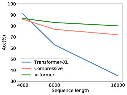
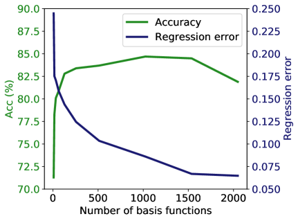
Figure 3: Left: Sorting task accuracy for sequences of length 4,000, 8,000, and 16,000. Right: Sorting task accuracy vs regression mean error, when varying the number of basis functions, for sequences of length 8,000.

In this task, the input consists of a sequence of tokens sampled according to a token probability distribution (which is not known to the system). The goal is to generate the tokens in the decreasing order of their frequencies in the sequence. One example can be:

$$\underbrace{1\;\;2\;\;1\;\;3\;\;1\;\;0\;\;3\;\;1\;\;3\;\;2\;\;}_{\text{$1$ occurs 4 times; $3$ occurs 3 times, etc.}}\textsc{<sep>}\;\;1\;\;3\;\;2\;\;0$$

To understand if the long-term memory is being effectively used and the transformer is not only performing sorting by modeling the most recent tokens, we design the token probability distribution to change over time: namely, we set it as a mixture of two distributions, ${p=\alpha p_{0}+(1-\alpha)p_{1}}$, where the mixture coefficient $\alpha\in[0,1]$ is progressively increased from 0 to 1 as the sequence is generated. The vocabulary has 20 tokens and we experiment with sequences of length 4,000, 8,000, and 16,000.

Baselines.

We consider the transformer-XL (Dai et al., 2019) and the compressive transformer (Rae et al., 2019) as baselines. The transformer-XL consists of a vanilla transformer (Vaswani et al., 2017) extended with a short-term memory which is composed of the hidden states of the previous steps. The compressive transformer is an extension of the transformer-XL: besides the short-term memory, it has a compressive long-term memory which is composed of the old vectors of the short-term memory, compressed using a CNN. Both the transformer-XL and the compressive transformer require relative positional encodings. In contrast, there is no need for positional encodings in the memory in our approach since the memory vectors represent basis coefficients in a predefined continuous space.

For all models we used a transformer with 3 layers and 6 attention heads, input size $L=1,024$ and memory size 2,048. For the compressive transformer, both memories have size 1,024. For the $\infty$-former, we also consider a STM of size 1,024 and a LTM with $N=1,024$ basis functions, having the models the same computational cost. Further details are described in App. C.1.

Results.

As can be seen in the left plot of Fig. 3, the transformer-XL achieves a slightly higher accuracy than the compressive transformer and $\infty$-former for a short sequence length (4,000). This is because the transformer-XL is able to keep almost the entire sequence in memory. However, its accuracy degrades rapidly when the sequence length is increased. Both the compressive transformer and $\infty$-former also lead to smaller accuracies when increasing the sequence length, as expected. However, this decrease is not so significant for the $\infty$-former, which indicates that it is better at modeling long sequences.

Regression error analysis.

To better understand the trade-off between the $\infty$-former’s memory precision and its computational efficiency, we analyze how its regression error and sorting accuracy vary when varying the number of basis functions used, on the sorting task with input sequences of length 8,000. As can be seen in the right plot of Fig. 3, the sorting accuracy is negatively correlated with the regression error, which is positively correlated with the number of basis functions. It can also be observed, that when increasing substantially the number of basis functions the regression error reaches a plateau and the accuracy starts to drop. We posit that the latter is caused by the model having a harder task at selecting the locations it should attend to. This shows that, as expected, when increasing $\infty$-former’s efficiency or increasing the size of context being modeled, the memory loses precision.

4.2 Language Modeling

To understand if long-term memories can be used to extend a pre-trained language model, we fine-tune GPT-2 small (Radford et al., 2019) on Wikitext-103 (Merity et al., 2017) and a subset of PG-19 (Rae et al., 2019) containing the first 2,000 books ($\approx$ 200 million tokens) of the training set. To do so, we extend GPT-2 with a continuous long-term memory ($\infty$-former) and a compressed memory (compressive transformer) with a positional bias, based on Press et al. (2021).

For these experiments, we consider transformers with input size $L=512$, for the compressive transformer we use a compressed memory of size 512, and for the $\infty$-former we consider a LTM with $N=512$ Gaussian RBFs and a memory threshold of 2,048 tokens, having the same computational budget for the two models. Further details and hyperparameters are described in App. C.2.

Results.

	Wikitext-103	PG19
GPT-2	16.85	33.44
Compressive	16.87	33.09
$\infty$-former	16.64	32.61
$\infty$-former (SM)	16.61	32.48

Table 1: Perplexity on Wikitext-103 and PG19.

The results reported in Table 1 show that the $\infty$-former leads to perplexity improvements on both Wikitext-103 and PG19, while the compressive transformer only has a slight improvement on the latter. The improvements obtained by the $\infty$-former are larger on the PG19 dataset, which can be justified by the nature of the datasets: books have more long range dependencies than Wikipedia articles (Rae et al., 2019).

4.3 Document Grounded Dialogue

In document grounded dialogue generation, besides the dialogue history, models have access to a document concerning the conversation’s topic. In the CMU Document Grounded Conversation dataset (CMU-DoG) (Zhou et al., 2018), the dialogues are about movies and a summary of the movie is given as the auxiliary document; the auxiliary document is divided into parts that should be considered for the different utterances of the dialogue. In this paper, to evaluate the usefulness of the long-term memories, we make this task slightly more challenging by only giving the models access to the document before the start of the dialogue.

We fine-tune GPT-2 small (Radford et al., 2019) using an approach based on Wolf et al. (2019). To allow the model to keep the whole document on memory, we extend GPT-2 with a continuous LTM ($\infty$-former) with $N=512$ basis functions. As baselines, we use GPT-2, with and without access (GPT-2 w/o doc) to the auxiliary document, with input size $L=512$, and GPT-2 with a compressed memory with attention positional biases (compressive), of size 512. Further details and hyper-parameters are stated in App. C.3.

To evaluate the models we use the metrics: perplexity, F1 score, Rouge-1 and Rouge-L (Lin, 2004), and Meteor (Banerjee and Lavie, 2005).

Results.

	PPL	F1	Rouge-1	Rouge-L	Meteor
GPT-2 w/o doc	19.43	7.82	12.18	10.17	6.10
GPT-2	18.53	8.64	14.61	12.03	7.15
Compressive	18.02	8.78	14.74	12.14	7.29
$\infty$-former	18.02	8.92	15.28	12.51	7.52
$\infty$-former (SM)	18.04	9.01	15.37	12.56	7.55

Table 2: Results on CMU-DoG dataset.

As shown in Table 2, by keeping the whole auxiliary document in memory, the $\infty$-former and the compressive transformer are able to generate better utterances, according to all metrics. While the compressive and $\infty$-former achieve essentially the same perplexity in this task, the $\infty$-former achieves consistently better scores on all other metrics. Also, using sticky memories leads to slightly better results on those metrics, which suggests that attributing a larger space in the LTM to the most relevant tokens can be beneficial.

Analysis.

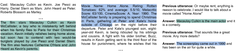
Figure 4: Examples of answers generated by $\infty$-former on a dialogue about the movie “Home Alone”. The excerpts from the LTM that are more attended to throughout the utterances generation are highlighted on each color, correspondingly.

Figure 5: Phrases that hold larger spaces of the LTM, when using sticky memories, for two dialogue examples (in App. E).

In Fig. 4, we show examples of utterances generated by $\infty$-former along with the excerpts from the LTM that receive higher attention throughout the utterances’ generation. In these examples, we can clearly see that these excerpts are highly pertinent to the answers being generated. Also, in Fig. 5, we can see that the phrases which are attributed larger spaces in the LTM, when using sticky memories, are relevant to the conversations.

5 Related Work

Continuous attention.

Martins et al. (2020) introduced 1D and 2D continuous attention, using Gaussians and truncated parabolas as densities. They applied it to RNN-based document classification, machine translation, and visual question answering. Several other works have also proposed the use of (discretized) Gaussian attention for natural language processing tasks: Guo et al. (2019) proposed a Gaussian prior to the self-attention mechanism to bias the model to give higher attention to nearby words, and applied it to natural language inference; You et al. (2020) proposed the use of hard-coded Gaussian attention as input-agnostic self-attention layer for machine translation; Dubois et al. (2020) proposed using Gaussian attention as a location attention mechanism to improve the model generalization to longer sequences. However, these approaches still consider discrete sequences and compute the attention by evaluating the Gaussian density at the token positions. Farinhas et al. (2021) extend continuous attention to multimodal densities, i.e., mixtures of Gaussians, and applied it to VQA. In this paper, we opt for the simpler case, an unimodal Gaussian, and leave sparse and multimodal continuous attention for future work.

Efficient transformers.

Several methods have been proposed that reduce the transformer’s attention complexity, and can, consequently, model longer contexts. Some of these do so by performing sparse attention, either by selecting pre-defined attention patterns (Child et al., 2019; Beltagy et al., 2020; Zaheer et al., 2020), or by learning these patterns from data (Kitaev et al., 2020; Vyas et al., 2020; Tay et al., 2020a; Roy et al., 2021; Wang et al., 2021). Other works focus on directly reducing the attention complexity by applying the (reversed) kernel trick (Katharopoulos et al., 2020; Choromanski et al., 2021; Peng et al., 2021; Jaegle et al., 2021). Closer to our approach are the transformer-XL and compressive transformer models (Dai et al., 2019; Rae et al., 2019), which extend the vanilla transformer with a bounded memory.

Memory-augmented language models.

RNNs, LSTMs, and GRUs (Hochreiter et al., 1997; Cho et al., 2014) have the ability of keeping a memory state of the past. However, these require backpropagation through time which is impractical for long sequences. Because of this, Graves et al. (2014), Weston et al. (2014), Joulin and Mikolov (2015) and Grefenstette et al. (2015) proposed extending RNNs with an external memory, while Chandar et al. (2016) and Rae et al. (2016) proposed efficient procedures to read and write from these memories, using hierarchies and sparsity. Grave et al. (2016) and Merity et al. (2017) proposed the use of cache-based memories which store pairs of hidden states and output tokens from previous steps. The distribution over the words in the memory is then combined with the distribution given by the language model. More recently, Khandelwal et al. (2019) and Yogatama et al. (2021) proposed using nearest neighbors to retrieve words from a key-based memory constructed based on the training data. Similarly, Fan et al. (2021) proposed retrieving sentences from a memory based on the training data and auxiliary information. Khandelwal et al. (2019) proposed interpolating the retrieved words probability distributions with the probability over the vocabulary words when generating a new word, while Yogatama et al. (2021) and Fan et al. (2021) proposed combining the information at the architecture level. These models have the disadvantage of needing to perform a retrieval step when generating each token / utterance, which can be computationally expensive. These approaches are orthogonal to the $\infty$-former’s LTM and in future work the two can be combined.

6 Conclusions

In this paper, we proposed the $\infty$-former: a transformer extended with an unbounded long-term memory. By using a continuous-space attention framework, its attention complexity is independent of the context’s length, which allows the model to attend to arbitrarily long contexts while keeping a fixed computation budget. By updating the memory taking into account past usage, the model keeps “sticky memories”, enforcing the persistence of relevant information in memory over time. Experiments on a sorting synthetic task show that $\infty$-former scales up to long sequences, maintaining a high accuracy. Experiments on language modeling and document grounded dialogue generation by fine-tuning a pre-trained language model have shown improvements across several metrics.

Ethics Statement

Transformer models that attend to long contexts, to improve their generation quality, need large amounts of computation and memory to perform self-attention. In this paper, we propose an extension to a transformer model that makes the attention complexity independent of the length of the context being attended to. This can lead to a reduced number of parameters needed to model the same context, which can, consequently, lead to gains in efficiency and reduce energy consumption.

On the other hand, the $\infty$-former, as well as the other transformer language models, can be used on questionable scenarios, such as the generation of fake news (Zellers et al., 2019), defamatory text (Wallace et al., 2019), or other undesired content.

Appendix A Multivariate ridge regression

The coefficient matrix $B\in\mathbb{R}^{N\times e}$ is obtained with multivariate ridge regression criterion so that $\bar{X}(t_{i})\approx x_{i}$ for each $i\in[L]$, which leads to the closed form:

$$B^{\top} =\operatorname*{arg\,min}_{B^{\top}}||B^{\top}F-X^{\top}||_{\mathcal{F}}^{2}+\lambda||B||_{\mathcal{F}}^{2}$$ (23)

$$=X^{\top}F^{\top}(FF^{\top}+\lambda I)^{-1}=X^{\top}G,$$

where $F=[\psi(t_{1}),\dots,\psi(t_{L})]$ packs the basis vectors for $L$ locations and $||\cdot||_{\mathcal{F}}$ is the Frobenius norm. As $G\in\mathbb{R}^{L\times N}$ only depends of $F$, it can be computed offline.

Appendix B Sticky memories

We present in Fig. 6 a scheme of the sticky memories procedure. First we sample $M$ locations from the previous step LTM attention histogram (Eq. 16). Then, we evaluate the LTM’s signal at the sampled locations (Eq. 14). Finally, we consider that the sampled vectors, $X_{\mathrm{past}}$, are linearly spaced in $[0,\tau]$. This way, the model is able to attribute larger spaces of its memory to the relevant words.

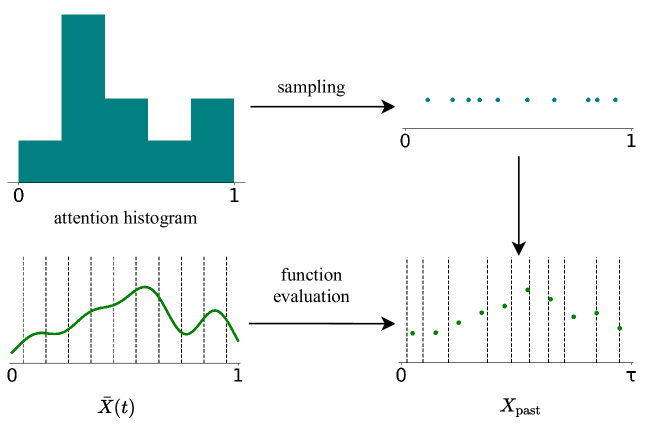
Figure 6: Sticky memories procedure diagram. The dashed vertical lines correspond to the position of the words in the LTM signal.

Appendix C Experimental details

C.1 Sorting

For the compressive transformer, we consider compression rates of size 2 for sequences of length 4,000, from $2$ to $6$ for sequences of length 8,000, and from $2$ to $12$ for sequences of length 16,000. We also experiment training the compressive transformer with and without the attention reconstruction auxiliary loss. For the $\infty$-former we consider 1,024 Gaussian RBFs $\mathcal{N}(t;\tilde{\mu},\tilde{\sigma}^{2})$ with $\tilde{\mu}$ linearly spaced in $[0,1]$ and $\tilde{\sigma}\in\{.01,.05\}$. We set $\tau=0.75$ and for the KL regularization we used $\lambda_{\mathrm{KL}}=1\times 10^{-5}$ and $\sigma_{0}=0.05$.

For this task, for each sequence length, we created a training set with 8,000 sequences and validation and test sets with 800 sequences. We trained all models with batches of size 8 for 20 epochs on 1 Nvidia GeForce RTX 2080 Ti or 1 Nvidia GeForce GTX 1080 Ti GPU with $\approx 11$ Gb of memory, using the Adam optimizer (Kingma and Ba, 2015). For the sequences of length 4,000 and 8,000 we used a learning rate of $2.5\times 10^{-4}$ while for sequences of length 16,000 we used a learning rate of $2\times 10^{-4}$. The learning rate was decayed to 0 until the end of training with a cosine schedule.

C.2 Pre-trained Language Models

In these experiments, we fine-tune the GPT-2 small, which is composed of 12 layers with 12 attention heads, on the English dataset Wikitext-103 and on a subset of the English dataset PG19 containing the first 2,000 books. We consider an input size $L=512$ and a long-term memory with $N=512$ Gaussian RBFs $\mathcal{N}(t;\tilde{\mu},\tilde{\sigma}^{2})$ with $\tilde{\mu}$ linearly spaced in $[0,1]$ and $\tilde{\sigma}\in\{.005,.01\}$ and for the KL regularization we use $\lambda_{\mathrm{KL}}=1\times 10^{-6}$ and $\sigma_{0}=0.05$. We set $\tau=0.5$. For the compressive transformer we also consider a compressed memory of size 512 with a compression rate of 4, and train the model with the auxiliary reconstruction loss.

We fine-tuned GPT-2 small with a batch size of 1 on 1 Nvidia GeForce RTX 2080 Ti or 1 Nvidia GeForce GTX 1080 Ti GPU with $\approx 11$ Gb of memory, using the Adam optimizer (Kingma and Ba, 2015) for 1 epoch with a learning rate of $5\times 10^{-5}$ for the GPT-2 parameters and a learning rate of $2.5\times 10^{-4}$ for the LTM parameters.

C.3 Document Grounded Generation

In these experiments, we fine-tune the GPT-2 small, which is composed of 12 layers with 12 attention heads, on the English dataset CMU - Document Grounded Conversations (CMU-DoG. CMU-DoG has 4112 conversations, being the proportion of train/validation/test split 0.8/0.05/0.15.

We consider an input size $L=512$ and a long-term memory with $N=512$ Gaussian RBFs $\mathcal{N}(t;\tilde{\mu},\tilde{\sigma}^{2})$ with $\tilde{\mu}$ linearly spaced in $[0,1]$ and $\tilde{\sigma}\in\{.005,.01\}$ and for the KL regularization we use $\lambda_{\mathrm{KL}}=1\times 10^{-6}$ and $\sigma_{0}=0.05$. We set $\tau=0.5$. For the compressive transformer we consider a compressed memory of size 512 with a compression rate of 3, and train the model with the auxiliary reconstruction loss. We fine-tuned GPT-2 small with a batch size of 1 on 1 Nvidia GeForce RTX 2080 Ti or 1 Nvidia GeForce GTX 1080 Ti GPU with $\approx 11$ Gb of memory, using the Adam optimizer (Kingma and Ba, 2015) with a linearly decayed learning rate of $5\times 10^{-5}$, for 5 epochs.

Appendix D Additional experiments

We also perform language modeling experiments on the Wikitext-103 dataset (Merity et al., 2017) which has a training set with 103 million tokens and validation and test sets with 217,646 and 245,569 tokens, respectively. For that, we follow the standard architecture of the transformer-XL (Dai et al., 2019), which consists of a transformer with 16 layers and 10 attention heads. For the transformer-XL, we experiment with a memory of size 150. For the compressive transformer, we consider that both memories have a size of 150 and a compression rate of 4. For the $\infty$-former we consider a short-term memory of size 150, a continuous long-term memory with 150 Gaussian RBFs, and a memory threshold of 900 tokens.

For this experiment, we use a transformer with 16 layers, 10 heads, embeddings of size 410, and a feed-forward hidden size of 2100. For the compressive transformer, we follow Rae et al. (2019) and use a compression rate of 4 and the attention reconstruction auxiliary loss. For the $\infty$-former we consider 150 Gaussian RBFs $\mathcal{N}(t;\tilde{\mu},\tilde{\sigma}^{2})$ with $\tilde{\mu}$ linearly spaced in $[0,1]$ and $\tilde{\sigma}\in\{.01,.05\}$. We set $\tau=0.5$ and for the KL regularization we used $\lambda_{\mathrm{KL}}=1\times 10^{-5}$ and $\sigma_{0}=0.1$.

We trained all models, from scratch, with batches of size 40 for 250,000 steps on 1 Nvidia Titan RTX or 1 Nvidia Quadro RTX 6000 with $\approx 24$ GPU Gb of memory using the Adam optimizer (Kingma and Ba, 2015) with a learning rate of $2.5\times 10^{-4}$. The learning rate was decayed to 0 until the end of training with a cosine schedule.

Results.

As can be seen in Table 3, extending the model with a long-term memory leads to a better perplexity, for both the compressive transformer and $\infty$-former. Moreover, the $\infty$-former slightly outperforms the compressive transformer. We can also see that using sticky memories leads to a somewhat lower perplexity, which shows that it helps the model to focus on the relevant memories.

	STM	LTM	Perplexity
Transformer-XL	150	—-	24.52
Compressive	150	150	24.41
$\infty$-former	150	150	24.29
$\infty$-former (Sticky memories)	150	150	24.22

Table 3: Perplexity on Wikitext-103.

Analysis.

To better understand whether $\infty$-former is paying more attention to the older memories in the LTM or to the most recent ones, we plotted a histogram of the attention given to each region of the long-term memory when predicting the tokens on the validation set. As can be seen in Fig. 7, in the first and middle layers, the $\infty$-former tends to focus more on the older memories, while in the last layer, the attention pattern is more uniform. In Figs. 8 and 9, we present examples of words for which the $\infty$-former has lower perplexity than the transformer-XL along with the attention given by the $\infty$-former to the last layer’s LTM. We can see that the word being predicted is present several times in the long-term memory and $\infty$-former gives higher attention to those regions.

To know whether the sticky memories approach attributes a larger space of the LTM’s signal to relevant phrases or words, we plotted the memory space given to each word present in the long-term memory of the last layer when using and not using sticky memories. We present examples in Figs. 10 and 11 along with the phrases / words which receive the largest spaces when using sticky memories. We can see in these examples that this procedure does in fact attribute large spaces to old memories, creating memories that stick over time. We can also see that these memories appear to be relevant as shown by the words / phrases in the examples.

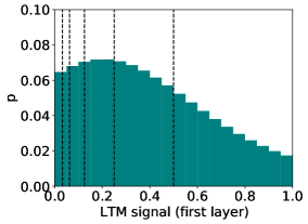
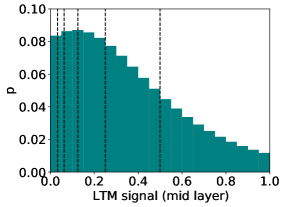
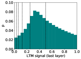
Figure 7: Histograms of attention given to the LTM by $\infty$-former, for the first (on the left), middle (on the middle), and last (on the right) layers. The dashed vertical lines represent the limits of the memory segments ($\tau$) for the various memory updates.

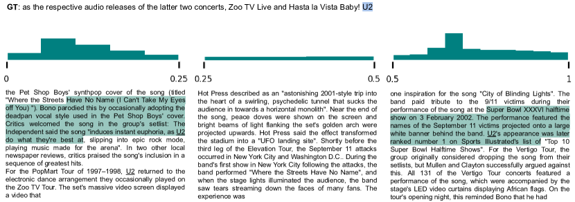
Figure 8: Example of attention given by $\infty$-former to the last layer’s long-term memory, when predicting the ground truth word “U2”. The words in the LTM which receive higher attention ($>0.05$) are shaded.

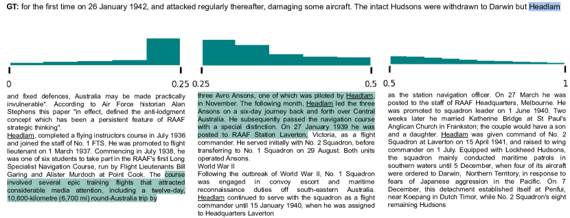
Figure 9: Example of attention given by $\infty$-former to the last layer’s long-term memory, when predicting the ground truth word “Headlam”. The words in the long-term memory which receive higher attention (bigger than $0.05$) are shaded.

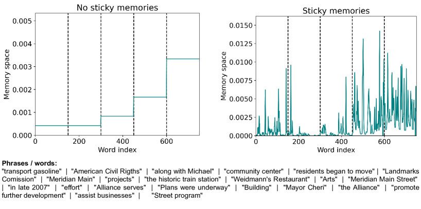
Figure 10: Example of the memory space attributed to each word in the last layer’s long-term memory (after 5 updates) without / with the sticky memories procedure, along with the words / phrases which have the largest memory spaces when using sticky memories (top peaks with space$>.005$). Excerpt of the sequence being generated in this example: “Given Meridian’s site as a railroad junction, its travelers have attracted the development of many hotels.” The dashed vertical lines represent the limits of the memory segments for the various memory updates.

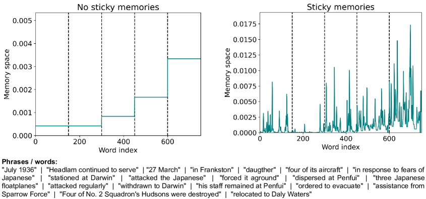
Figure 11: Example of the memory space attributed to each word in the last layer’s long-term memory (after 5 updates) without / with the sticky memories procedure, along with the words / phrases which have the largest memory spaces when using sticky memories (top peaks with space$>.005$) Excerpt of the sequence being generated in this example: “Headlam became Officer Commanding North-Western Area in January 1946. Posted to Britain at the end of the year, he attended the Royal Air Force Staff College, Andover, and served with RAAF Overseas Headquarters, London.” The dashed vertical lines represent the limits of the memory segments for the various memory updates.

Appendix E Additional examples

In Fig. 12, we show additional examples of utterances generated by $\infty$-former along with the excerpts from the LTM that receive higher attention throughout the utterances’ generation.

Additionally, ground truth conversations concerning the movies “Toy Story” and “La La Land”, for which the sticky memories are stated in Fig. 5, are shown in Tables 4 and 5, respectively.

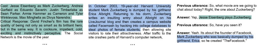
Figure 12: Examples of answers generated by $\infty$-former on a dialogue about the movie “The Social Network”. The excerpts from the LTM that are more attended to throughout their generation are highlighted on each color correspondingly.

- Hi

- Yo you really need to watch Toy Story. It has 100% on Rotten Tomatoes!

- Really! 100% that’s pretty good What’s it about

- It’s an animated buddy-comedy where toys come to life

- who stars in it

- The main characters are voiced by Tom Hanks and Tim Allen

- does it have any other critic ratings

- Yep, metacritic gave it 95/100 and Cinemascore gave it an A

- how old is it?

- It’s a 1995 film so 23 years

- The old ones are always good :) I heard there were some sad parts in it is that true

- Yeah actually, the movie starts off pretty sad as the toys fear that they might be replaced and that they have to move

- is this a disney or dreamworks movie

- Disney, pixar to be exact

- Why do the toys think they will be replaced :(

- they thought so because Andy was having a birthday party and might get new toys

- What part does Tom Hanks play

- Woody, the main character

- How about Tim Allen

- Buzz, the main antagonist at first then he becomes a friend

- What kind of toy is Woody?

- A cowboy doll

- What is Buzz

- A space ranger

- so do all the toys talk

- yep! but andy doesn’t know that

- Is andy a little kid or a teen

- He’s 6!

- Sounds good. Thanks for the info. Have a great day

Table 4: Ground truth conversation about movie “Toy Story”.

- hey

- hey

- i just watched la la land. It is a movie from 2016 starring ryan gosling and emma stone. they are too artists (one actress and one panist) and they fall in love and try to achieve their dreams. its a great movie

- It’s a wonderful movie and got a score of 92% on rotten tomatoes

- yes, i think it also won an oscar

- Yes but I thought it was a little dull

- metacritics rating is 93/100 as well its pretty critically acclaimed

- the two leads singing and dancing weren’t exceptional

- i suppose it is not for everyone

- It also sags badly in the middle I like how Sebastian slipped into a passionate jazz despite warnings from the owner.

- what do you think of the cover of "i ran so far away?" in the movie, sebastian found the song an insult for a serious musician

- I don’t know, it is considered an insult for serious musicians not sure why

- yeah

- The idea of a one woman play was daring

- it was interesting how sebastian joined a jazz fusion band he couldnt find real happiness in any of the bands he was in its hard

- It is considering she didn’t know of any of that until she attended one of his concerts

- yeah, that is daring the movie kind of speaks to a lot of people. she accussed him of abandoning his dreams but sometimes thats what you have to do.

- Not nice that she leaves because he told her she liked him better when he was unsuccessful The play was a disaster so he didn’t miss anything when he missed it.

- yeah, but i dont blame her for dumping him for that

- She should didn’t want to support him and she had to move back

- id be pretty upset as well to boulder city nevada

- yes she didn’t want to forgive him, I didn’t understand that

- well because that was a big deal to her and he missed it

- if she was with him when he was unsuccessful, she could have supported him to follow his dreams or other dreams

- i suppose that is true

- she wasn’t successful either

- yeah she wasnt nobody showed up to her play

- so why the big hulabaloo about him

- not sure

- she was selfish I guess He missed her play because he had to go for a photo shoot with the band that he had previously missed

- yeah but he should have kept better track and scheduled it better

- this shows that he was trying to commit some and follow his dreams although not necessarily like them so she would be please if he didn’t attend the photo shoot a second time, and came to her show

- i definitely felt bad for both of them though in that scene

- it’s more of a do or don’t he is still condemned I feel bad for him because he tried he tried to get her back by apologizing as well she didn’t want any of it

- yeah because she felt like he didnt care enough because he missed it he’s the one that suggested the one woman play

- They could have started all over again just like the beginning

- maybe so

- did she fail because of the one-woman play? she could have tried something else if she felt that

- she wanted to give it a shot

- she did and it failed, he did and it failed they just had to compromise so they could be together again, which was how the happiness was He signed up for the band after hearing her talking to her mom about how he is working

- on his career I think he did a lot for her

Table 5: Ground truth conversation about movie “La La Land”.

References

- Ba et al. (2016) Jimmy Lei Ba, Jamie Ryan Kiros, and Geoffrey E Hinton. 2016. Layer normalization.
- Bamji (2005) Shernaz X Bamji. 2005. Cadherins: actin with the cytoskeleton to form synapses. Neuron.
- Banerjee and Lavie (2005) Satanjeev Banerjee and Alon Lavie. 2005. METEOR: An automatic metric for MT evaluation with improved correlation with human judgments. In Proc. Workshop on intrinsic and extrinsic evaluation measures for machine translation and/or summarization.
- Beltagy et al. (2020) Iz Beltagy, Matthew E Peters, and Arman Cohan. 2020. Longformer: The long-document transformer.
- Brown et al. (1980) Philip J Brown, James V Zidek, et al. 1980. Adaptive multivariate ridge regression. The Annals of Statistics.
- Brown et al. (2020) Tom B Brown, Benjamin Mann, Nick Ryder, Melanie Subbiah, Jared Kaplan, Prafulla Dhariwal, Arvind Neelakantan, Pranav Shyam, Girish Sastry, Amanda Askell, et al. 2020. Language Models are Few-Shot Learners. In Proc. NeurIPS.
- Carroll (2007) D.W. Carroll. 2007. Psychology of Language. Cengage Learning.
- Chandar et al. (2016) Sarath Chandar, Sungjin Ahn, Hugo Larochelle, Pascal Vincent, Gerald Tesauro, and Yoshua Bengio. 2016. Hierarchical memory networks.
- Child et al. (2019) Rewon Child, Scott Gray, Alec Radford, and Ilya Sutskever. 2019. Generating long sequences with sparse transformers.
- Cho et al. (2014) Kyunghyun Cho, Bart van Merriënboer, Dzmitry Bahdanau, and Yoshua Bengio. 2014. On the Properties of Neural Machine Translation: Encoder–Decoder Approaches. In Proc. Workshop on Syntax, Semantics and Structure in Statistical Translation.
- Choromanski et al. (2021) Krzysztof Choromanski, Valerii Likhosherstov, David Dohan, Xingyou Song, Andreea Gane, Tamas Sarlos, Peter Hawkins, Jared Davis, Afroz Mohiuddin, Lukasz Kaiser, et al. 2021. Rethinking attention with performers. In Proc. ICLR (To appear).
- Dai et al. (2019) Zihang Dai, Zhilin Yang, Yiming Yang, William W Cohen, Jaime Carbonell, Quoc V Le, and Ruslan Salakhutdinov. 2019. Transformer-xl: Attentive language models beyond a fixed-length context. In Proc. ACL.
- Dubois et al. (2020) Yann Dubois, Gautier Dagan, Dieuwke Hupkes, and Elia Bruni. 2020. Location Attention for Extrapolation to Longer Sequences. In Proc. ACL.
- Fan et al. (2021) Angela Fan, Claire Gardent, Chloé Braud, and Antoine Bordes. 2021. Augmenting Transformers with KNN-Based Composite Memory for Dialog. Transactions of the Association for Computational Linguistics.
- Farinhas et al. (2021) António Farinhas, André F. T. Martins, and P. Aguiar. 2021. Multimodal Continuous Visual Attention Mechanisms.
- Grave et al. (2016) Edouard Grave, Armand Joulin, and Nicolas Usunier. 2016. Improving Neural Language Models with a Continuous Cache. In Proc. ICLR.
- Graves et al. (2014) Alex Graves, Greg Wayne, and Ivo Danihelka. 2014. Neural turing machines.
- Grefenstette et al. (2015) Edward Grefenstette, Karl Moritz Hermann, Mustafa Suleyman, and Phil Blunsom. 2015. Learning to transduce with unbounded memory. Proc. NeurIPS.
- Guo et al. (2019) Maosheng Guo, Yu Zhang, and Ting Liu. 2019. Gaussian Transformer: A Lightweight Approach for Natural Language Inference. In Proc. AAAI.
- He et al. (2016) Kaiming He, Xiangyu Zhang, Shaoqing Ren, and Jian Sun. 2016. Deep residual learning for image recognition. In Proc. CVPR.
- Hochreiter et al. (1997) Sepp Hochreiter, J urgen Schmidhuber, and Corso Elvezia. 1997. Long Short-Term Memory. Neural Computation.
- Jaegle et al. (2021) Andrew Jaegle, Felix Gimeno, Andrew Brock, Andrew Zisserman, Oriol Vinyals, and Joao Carreira. 2021. Perceiver: General Perception with Iterative Attention.
- Joulin and Mikolov (2015) Armand Joulin and Tomas Mikolov. 2015. Inferring algorithmic patterns with stack-augmented recurrent nets. Proc. NeurIPS.
- Katharopoulos et al. (2020) Angelos Katharopoulos, Apoorv Vyas, Nikolaos Pappas, and François Fleuret. 2020. Transformers are rnns: Fast autoregressive transformers with linear attention. In Proc. ICML.
- Khandelwal et al. (2019) Urvashi Khandelwal, Omer Levy, Dan Jurafsky, Luke Zettlemoyer, and Mike Lewis. 2019. Generalization through Memorization: Nearest Neighbor Language Models. In Proc. ICLR.
- Kingma and Ba (2015) Diederik P Kingma and Jimmy Ba. 2015. Adam: A Method for Stochastic Optimization. In Proc. ICLR.
- Kitaev et al. (2020) Nikita Kitaev, Łukasz Kaiser, and Anselm Levskaya. 2020. Reformer: The efficient transformer. In Proc. ICLR.
- Kuhbandner (2020) Christof Kuhbandner. 2020. Long-Lasting Verbatim Memory for the Words of Books After a Single Reading Without Any Learning Intention. Frontiers in Psychology.
- Lin (2004) Chin-Yew Lin. 2004. Rouge: A package for automatic evaluation of summaries. In Proc. Workshop on Automatic Summarization.
- Martins et al. (2020) André FT Martins, Marcos Treviso, António Farinhas, Vlad Niculae, Mário AT Figueiredo, and Pedro MQ Aguiar. 2020. Sparse and Continuous Attention Mechanisms. In Proc. NeurIPS.
- Merity et al. (2017) Stephen Merity, Caiming Xiong, James Bradbury, and Richard Socher. 2017. Pointer Sentinel Mixture Models. In Proc. ICLR.
- Mills et al. (2014) Fergil Mills, Thomas E Bartlett, Lasse Dissing-Olesen, Marta B Wisniewska, Jacek Kuznicki, Brian A Macvicar, Yu Tian Wang, and Shernaz X Bamji. 2014. Cognitive flexibility and long-term depression (LTD) are impaired following -catenin stabilization in vivo. In Proc. of the National Academy of Sciences.
- Peng et al. (2021) Hao Peng, Nikolaos Pappas, Dani Yogatama, Roy Schwartz, Noah Smith, and Lingpeng Kong. 2021. Random Feature Attention. In Proc. ICLR (To appear).
- Press et al. (2021) Ofir Press, Noah A Smith, and Mike Lewis. 2021. Train short, test long: Attention with linear biases enables input length extrapolation.
- Radford et al. (2018) Alec Radford, Karthik Narasimhan, Tim Salimans, and Ilya Sutskever. 2018. Improving language understanding by generative pre-training.
- Radford et al. (2019) Alec Radford, Jeffrey Wu, Rewon Child, David Luan, Dario Amodei, and Ilya Sutskever. 2019. Language models are unsupervised multitask learners.
- Rae et al. (2016) Jack W Rae, Jonathan J Hunt, Tim Harley, Ivo Danihelka, Andrew Senior, Greg Wayne, Alex Graves, and Timothy P Lillicrap. 2016. Scaling memory-augmented neural networks with sparse reads and writes. In Proc. NeurIPS.
- Rae et al. (2019) Jack W Rae, Anna Potapenko, Siddhant M Jayakumar, Chloe Hillier, and Timothy P Lillicrap. 2019. Compressive Transformers for Long-Range Sequence Modelling. In Proc. ICLR.
- Roy et al. (2021) Aurko Roy, Mohammad Saffar, Ashish Vaswani, and David Grangier. 2021. Efficient content-based sparse attention with routing transformers. Transactions of the Association for Computational Linguistics, 9:53–68.
- Tay et al. (2020a) Yi Tay, Dara Bahri, Liu Yang, Donald Metzler, and Da-Cheng Juan. 2020a. Sparse sinkhorn attention. In Proc. ICML.
- Tay et al. (2020b) Yi Tay, Mostafa Dehghani, Dara Bahri, and Donald Metzler. 2020b. Efficient transformers: A survey.
- Vaswani et al. (2017) Ashish Vaswani, Noam Shazeer, Niki Parmar, Jakob Uszkoreit, Llion Jones, Aidan N Gomez, Łukasz Kaiser, and Illia Polosukhin. 2017. Attention is all you need. In Proc. NeurIPS.
- Vyas et al. (2020) Apoorv Vyas, Angelos Katharopoulos, and François Fleuret. 2020. Fast transformers with clustered attention. In Proc. NeurIPS.
- Wallace et al. (2019) Eric Wallace, Shi Feng, Nikhil Kandpal, Matt Gardner, and Sameer Singh. 2019. Universal Adversarial Triggers for Attacking and Analyzing NLP. In Proc. EMNLP-IJCNLP.
- Wang et al. (2021) Shuohang Wang, Luowei Zhou, Zhe Gan, Yen-Chun Chen, Yuwei Fang, Siqi Sun, Yu Cheng, and Jingjing Liu. 2021. Cluster-Former: Clustering-based Sparse Transformer for Question Answering. In Proc. ACL Findings.
- Weston et al. (2014) Jason Weston, Sumit Chopra, and Antoine Bordes. 2014. Memory networks.
- Wolf et al. (2019) Thomas Wolf, Victor Sanh, Julien Chaumond, and Clement Delangue. 2019. Transfertransfo: A transfer learning approach for neural network based conversational agents.
- Yogatama et al. (2021) Dani Yogatama, Cyprien de Masson d’Autume, and Lingpeng Kong. 2021. Adaptive Semiparametric Language Models. Transactions of the Association for Computational Linguistics, 9:362–373.
- You et al. (2020) Weiqiu You, Simeng Sun, and Mohit Iyyer. 2020. Hard-Coded Gaussian Attention for Neural Machine Translation. In Proc. ACL.
- Zaheer et al. (2020) Manzil Zaheer, Guru Guruganesh, Avinava Dubey, Joshua Ainslie, Chris Alberti, Santiago Ontanon, Philip Pham, Anirudh Ravula, Qifan Wang, Li Yang, et al. 2020. Big bird: Transformers for longer sequences.
- Zellers et al. (2019) Rowan Zellers, Ari Holtzman, Hannah Rashkin, Yonatan Bisk, Ali Farhadi, Franziska Roesner, and Yejin Choi. 2019. Defending against neural fake news. Proc. NeurIPS.
- Zhou et al. (2018) Kangyan Zhou, Shrimai Prabhumoye, and Alan W Black. 2018. A Dataset for Document Grounded Conversations. In Proc. EMNLP.