Sparse principal component analysis for high-dimensional stationary time series

Abstract

We consider the sparse principal component analysis for high-dimensional stationary processes. The standard principal component analysis performs poorly when the dimension of the process is large. We establish the oracle inequalities for penalized principal component estimators for the processes including heavy-tailed time series. The rate of convergence of the estimators is established. We also elucidate the theoretical rate for choosing the tuning parameter in penalized estimators. The performance of the sparse principal component analysis is demonstrated by numerical simulations. The utility of the sparse principal component analysis for time series data is exemplified by the application to average temperature data.

1 Introduction.

The principal component analysis (PCA) has been a standard tool for multivariate data analysis. It facilitates the understanding of the covariance matrix and becomes a central method for dimension reduction and variable selection. When the sample size is large, Anderson (1963) developed the asymptotic theory for principal component analysis. A thorough investigation into the standard principal component analysis is summarized in Jolliffe (2002).

The dimension $p$ of the contemporary data is often large, compared with the sample size. Johnstone (2001) investigated the distribution of the largest eigenvalue when $p$ is large, and introduced the concept of the spiked covariance matrix model. The sparse principal component analysis, combined with variable selection techniques such as Lasso (Tibshirani (1996) or elastic net Zou and Hastie (2005)), was introduced in Zou et al. (2006). Shen and Huang (2008) considered the sparse principal component analysis via regularized low-rank matrix approximation. Johnstone and Lu (2009) provided a simple algorithm for selecting a subset of coordinates with the largest sample variances with consistency even when the dimension $p$ is large. Amini and Wainwright (2009) proposed two computational methods for recovering the support set of the leading eigenvector in the spiked covariance model. Cai and Zhou (2012) derived the optimal rates of convergence for sparse covariance matrix estimation. Paul and Johnstone (2012) proposed an augmented sparse PCA method and showed that the procedure attains near optimal rate of convergence. Birnbaum et al. (2013) studied the problem of estimating the leading eigenvector under the $l_{2}$-loss for independent high-dimensional Gaussian observations. Cai et al. (2013) considered both minimax and adaptive estimation of the principal subspace in the high dimensional setting. Vu and Lei (2013) also considered the sparse principal subspace estimation problems and established the optimal bounds for row subspace and nearly optimal for column subspace. Berthet and Rigollet (2013) derived a minimax optimality in a finite sample analysis for sparse principal components of a high-dimensional covariance matrix. In view of computation of the sparse principal component analysis, the several work has been appeared. For example, Ma (2013) proposed the iterative thresholding method for estimation of the leading eigenvector, and Wang et al. (2016) studied the computationally efficient algorithm to estimate the principal subspace. van de Geer (2016) formalized the theoretical development for sparse PCA on some local set, which is induced to ensure the compatibility condition (See also, e.g. Bühlmann and van de Geer (2011)). Notably, much of the above theory was developed under the setting of i.i.d. observations.

The principal component analysis applied to dependent data has also been studied for a long time. Zhao et al. (1986) proposed a new procedure for detection of signals based on eigenvalues of covariance matrix. Taniguchi and Krishnaiah (1987) derived the asymptotic distributions of eigenvalues of the sample covariance matrix from Gaussian stationary processes. However, all these developments are restricted to the case when the dimension $p$ is finite, i.e., the PCA for multivariate stationary processes. More details of analyses for multivariate stationary processes can be found in Taniguchi and Kakizawa (2000). The limiting distribution of sample covariance matrix for large-dimensional linear models was derived in Jin et al. (2009). The Marčenko-Pastur theorem for time series was obtained in an explicit way in Yao (2012). The high-dimensional covariance estimation for dependent data with some regularization techniques was introduced in Pourahmadi (2013). The theoretical development for regularized estimation in sparse high-dimensional time series models was considered in Basu and Michailidis (2015). They showed that a restricted eigenvalue condition holds with high probability. Motivated by this work, Wong et al. (2020) established the consistency of Lasso for some sparse non-Gaussian and nonlinear time series.

In this paper, we consider the sparse principal component analysis for high-dimensional stationary time series. Especially, we established the oracle inequalities for the Lasso-type PCA estimator for both $\alpha$-mixing Gaussian process and $\beta$-mixing sub-Weibull process. In addition, we also derived the oracle inequality for $l_{0}$-penalized estimators for comparison. The finite sample performance is illustrated by some numerical simulations.

1.1 Notation.

For a vector $\bm{v}\in\mathbb{R}^{p}$, we defined the $l_{r}$-norm $\|\bm{v}\|_{r}$ as $\|\bm{v}\|_{r}=\left(\sum_{i=1}^{p}|v_{i}|^{r}\right)^{1/r}$ for $r\in(0,\infty)$. Also, let $\|\bm{v}\|_{0}$ and $\|\bm{v}\|_{\infty}$ be $\|\bm{v}\|_{0}=\sum_{i=1}^{p}\mathbbm{1}_{\{|v_{i}|>0\}}$ and $\|\bm{v}\|_{\infty}=\max_{1\leq i\leq p}|v_{i}|$, respectively.

For a $p\times p$ matrix $A$, the operator norm $\|A\|_{r}$ is defined as

$$\|A\|_{r}:=\sup_{\|v\|_{r}=1}\|A\bm{v}\|_{r},\quad r\in(0,\infty].$$

Moreover, the “max” norm of the matrix $A$ is $\|A\|_{\max}:=\max_{i,j}|A_{ij}|$. For a vector $\bm{v}\in\mathbb{R}^{p}$, and an index set $T\subset\{1,2,\ldots,p\}$, we denote by $\bm{v}_{T}$ the $|T|$-dimensional sub-vector of $\bm{v}$ restricted by the index set $T$, where $|T|$ is the number of elements of the set $T$.

The rest of the paper is organized as follows. In Section 2, we provide the fundamental settings for the sparse principal component analysis for stationary processes. Theoretical results of the Lasso-type principal component analysis for Gaussian processes and heavy-tailed processes are discussed in Sections 3 and 4, respectively. In addition, the $l_{0}$-penalized estimation is discussed in Section 5. Section 6 gives several simulation results to demonstrate the finite sample performance of sparse principal component analyses. The rigorous proofs and technical results are relegated to Section 7.

2 Preliminaries.

2.1 Model setups.

Let $\{\bm{X}_{t}\}_{t\in\mathbb{Z}}$ be an $\mathbb{R}^{p}$-valued, strictly stationary, and centered time series on a probability space $(\Omega,\mathcal{F},P)$. Suppose the observation stretch $(\bm{X}_{1},\ldots,\bm{X}_{n}),\ n\in\mathbb{N}$, is available. Consider the following $p\times p$ matrices

$$\Sigma_{0}=E[\bm{X}_{t}\bm{X}_{t}^{\top}],\qquad\qquad\hat{\Sigma}_{n}=\frac{1}{n}\sum_{t=1}^{n}\bm{X}_{t}\bm{X}_{t}^{\top}.$$

Let $\bm{q}^{0}$ be the first principal component corresponding to the largest eigenvalue $\phi_{\max}^{2}:=\Lambda_{\max}(\Sigma_{0})$ of $\Sigma_{0}$, so that $\bm{q}^{0}$ is normalized as $\|\bm{q}^{0}\|_{2}=1$. The parameter of interest is

$$\bm{\beta}^{0}=\phi_{\max}\bm{q}^{0},$$

which is a solution to the following optimization problem

$$\bm{\beta}^{0}=\arg\min_{\bm{\beta}\in\mathbb{R}^{p}}\frac{1}{4}\|\Sigma_{0}-\bm{\beta}\bm{\beta}^{\top}\|_{F}^{2},$$

where $\|\cdot\|_{F}$ is the Frobenius norm. In other words, it holds that

$$\Sigma_{0}\bm{\beta}^{0}=\phi_{\max}^{2}\bm{\beta}^{0}=\|\bm{\beta}^{0}\|_{2}^{2}\bm{\beta}^{0}.$$

Our primary interest is the sparse principal component estimation. Let $S$ be $S=\{j:\bm{\beta}^{0}_{j}\not=0\}$. Specifically, $\bm{\beta}^{0}$ is supposed to be $s_{0}$-sparse, $i.e.,$ $|S|=s_{0}$. A typical motivating example is given as follows.

Example 1.

Consider the stationary process $\{\bm{X}_{t}\}$ taking the form of VAR model, i.e.,

$$\bm{X}_{t}=A\bm{X}_{t-1}+\bm{\epsilon}_{t},\qquad\bm{\epsilon_{t}}\sim{\rm i.i.d.}(\bm{0},I_{p}),$$ (2.1)

where $A$ is a $p\times p$ deterministic matrix with the decomposition

$$A=\sum_{j=1}^{p}\nu_{j}\bm{p}_{j}\bm{p}_{j}^{\top}$$

such that $1>\nu_{1}\geq\cdots\geq\nu_{p}\geq 0$ are the eigenvalues of $A$, with $\bm{p}_{j}$ the associated eigenvectors. Suppose the eigenvector $\bm{p}_{1}$ is $s_{0}$-sparse. By the holomorphic functional calculus, we have

$$\Sigma_{0}=\sum_{j=1}^{p}\frac{1}{1-\nu_{j}^{2}}\bm{p}_{j}\bm{p}_{j}^{\top},$$

which shows that the first principal component of $\Sigma_{0}$ is also $s_{0}$-sparse.

In this paper, we consider the following penalized PCA estimators. In such a high-dimensional setting, the sparse estimation is essential for variable selection, which facilitates the interpretation of features in the dataset.

Definition 2.1.

The following estimator for $\bm{\beta}^{0}$ is defined as

$$\hat{\bm{\beta}}_{n}:=\arg\min_{\beta\in\mathcal{B}}\left\{\frac{1}{4}\|\hat{\Sigma}_{n}-\bm{\beta}\bm{\beta}^{\top}\|_{F}^{2}+\lambda\,{\rm pen}(\bm{\beta})\right\},\quad\mathcal{B}:=\{\bm{\beta}:\|\bm{\beta}-\bm{\beta}^{0}\|_{2}\leq\eta\},$$

where $\lambda\geq 0$ is a tuning parameter, ${\rm pen}(\cdot)$ is some penalty function, and $\eta>0$ is a suitable constant. The following estimators are focused on in this paper. The $l_{1}$-penalized estimator $\hat{\bm{\beta}}_{n}^{1}$ is defined as

$$\hat{\bm{\beta}}_{n}^{1}:=\arg\min_{\beta\in\mathcal{B}}\left\{\frac{1}{4}\|\hat{\Sigma}_{n}-\bm{\beta}\bm{\beta}^{\top}\|_{F}^{2}+\lambda_{1}\|\bm{\beta}\|_{1}\right\},$$ (2.2)

where $\lambda=\lambda_{1}$ and ${\rm pen}(\bm{\beta})=\|\bm{\beta}\|_{1}$. The estimator $\hat{\bm{\beta}}_{n}^{1}$ is also referred to as the Lasso-type estimator. The $l_{0}$-penalized estimator $\hat{\bm{\beta}}_{n}^{0}$ is defined as

$$\hat{\bm{\beta}}_{n}^{0}:=\arg\min_{\beta\in\mathcal{B}}\left\{\frac{1}{4}\|\hat{\Sigma}_{n}-\bm{\beta}\bm{\beta}^{\top}\|_{F}^{2}+\lambda_{0}\|\bm{\beta}\|_{0}\right\},$$ (2.3)

where $\lambda=\lambda_{0}$ and ${\rm pen}(\bm{\beta})=\|\bm{\beta}\|_{0}$.

We establish the error bound of the estimator $\hat{\bm{\beta}}_{n}$ for high-dimensional time series. In the following, we list the definition of mixing coefficients for stochastic processes.

Definition 2.2.

For a stationary process $\{\bm{X}_{t}\}_{t\in\mathbb{Z}}$, we define the following quantities.

• The $\alpha$-mixing coefficients for $\{\bm{X}_{t}\}_{t\in\mathbb{Z}}$ is defined as

  $$\alpha(l) := \sup\{|P(A\cap B)-P(A)P(B)|:$$

  $$A\in\sigma(\bm{X}_{s},\ s\leq t),\ B\in\sigma(\bm{X}_{s},\ s\geq t+l)\ \mbox{for all}\ t\in\mathbb{Z}\},\quad l\in\mathbb{Z}.$$

  The process $\{\bm{X}_{t}\}_{t\in\mathbb{Z}}$ is called $\alpha$-mixing if $\alpha(l)\to 0$ as $l\to\infty$.

• The $\rho$-mixing coefficients for $\{\bm{X}_{t}\}_{t\in\mathbb{Z}}$ is defined as

  $$\rho(l) := \sup\{\mathop{\rm Cov}\nolimits(f(\bm{X}_{t}),g(\bm{X}_{t+l})):$$

  $$E[f]=E[g]=0,\ E[f^{2}]=E[g^{2}]=1\},\quad l\in\mathbb{Z}.$$

  The process $\{\bm{X}_{t}\}_{t\in\mathbb{Z}}$ is called $\rho$-mixing if $\rho(l)\to 0$ as $l\to\infty$.

• The $\beta$-mixing coefficients for $\{\bm{X}_{t}\}_{t\in\mathbb{Z}}$ is defined by

  $$\beta(l) := \sup\frac{1}{2}\sum_{i=1}^{I}\sum_{j=1}^{J}|P(A\cap B)-P(A)P(B)|,\quad l\in\mathbb{Z},$$

  where the supremum is over all pair of partitions $\{A_{i}\}_{1\leq i\leq I}\subset\sigma(\bm{X}_{s},\ s\leq t)$ and $\{B_{j}\}_{1\leq j\leq J}\subset\sigma(\bm{X}_{s},\ s\geq t+l)$. The process $\{\bm{X}_{t}\}_{t\in\mathbb{Z}}$ is called $\beta$-mixing if $\beta(l)\to 0$ as $l\to\infty$.

All these conditions are known as the weak dependence conditions (e.g. Tikhomirov (1981)), under which the convergence rate in the central limit theorem for weakly dependent random variables is evaluated.

Now consider the spectral decomposition of $\Sigma_{0}$ as

$$\Sigma_{0}=U\Phi_{0}U^{\top},$$

where $\Phi_{0}^{2}:=\mathop{\rm diag}(\phi_{1}^{2},\ldots,\phi_{p}^{2})$ with $\phi_{1}\geq\ldots\geq\phi_{p}\geq 0$ is a diagonal matrix constructed by the eigenvalues of $\Sigma_{0}$, and $U=(\bm{u}_{1},\ldots,\bm{u}_{p})$ satisfies that $UU^{\top}=U^{\top}U=I_{p}$. Actually, we have $\phi_{\max}=\phi_{1}$ and $\bm{q}^{0}=\bm{u}_{1}$. Hereafter, we assume the following conditions.

Assumption 2.3.

Suppose that the dimension $p:=p(n)$ of the process $\{\bm{X}_{t}\}$ satisfies $\log p/n=o(1)$ as $n\to\infty$. There exists a constant $\sigma>3\eta>0$ such that

$$\phi_{\max}\geq\phi_{j}+\sigma,\quad j\geq 2.$$

The second condition separates the largest eigenvalue from other eigenvalues.

2.2 Risk functions.

We define the theoretical risk $R(\cdot)$ and empirical risk $R_{n}(\cdot)$ and their derivatives with respect to $\bm{\beta}$ as follows:

$$R(\bm{\beta}):=-\frac{1}{2}\bm{\beta}^{\top}\Sigma_{0}\bm{\beta}+\frac{1}{4}\|\bm{\beta}\|_{2}^{4},\quad R_{n}(\bm{\beta}):=-\frac{1}{2}\bm{\beta}^{\top}\hat{\Sigma}_{n}\bm{\beta}+\frac{1}{4}\|\bm{\beta}\|_{2}^{4},$$

$$\dot{R}(\bm{\beta})=-\Sigma_{0}\bm{\beta}+\|\bm{\beta}\|_{2}^{2}\bm{\beta},\quad\dot{R}_{n}(\bm{\beta})=-\hat{\Sigma}_{n}\bm{\beta}+\|\bm{\beta}\|_{2}^{2}\bm{\beta},$$

and

$$\ddot{R}(\bm{\beta}):=-\Sigma_{0}+\|\bm{\beta}\|_{2}^{2}I_{p}+2\bm{\beta}\bm{\beta}^{\top},\quad\ddot{R}_{n}(\bm{\beta}):=-\hat{\Sigma}_{n}+\|\bm{\beta}\|_{2}^{2}I_{p}+2\bm{\beta}\bm{\beta}^{\top}.$$

Then, it holds that

$$\bm{\beta}^{0}=\arg\min_{\bm{\beta}\in\mathbb{R}^{p}}R(\bm{\beta}),\quad\hat{\bm{\beta}}_{n}=\arg\min_{\bm{\beta}\in\mathcal{B}}\left\{R_{n}(\bm{\beta})+\lambda\,{\rm pen}(\bm{\beta})\right\}.$$

For brevity, we denote $W_{n}=\hat{\Sigma}_{n}-\Sigma_{0}$. Note that

$$\dot{R}_{n}(\bm{\beta})-\dot{R}(\bm{\beta})=-W_{n}\bm{\beta}$$

and that

$$\ddot{R}_{n}(\bm{\beta})-\ddot{R}(\bm{\beta})=-W_{n}.$$

The following result holds for the risk function.

Proposition 2.1 (Lemma 12.7, van de Geer (2016)).

Under Assumption 2.3, $\ddot{R}(\bm{\beta})$ is positive definite on $\bm{\beta}\in\mathcal{B}$.

By Proposition 2.1, the theoretical risk function $R(\cdot)$ is shown to be strictly convex on $\mathcal{B}$. This motivates us to consider the penalized PCA estimators as an optimization problem. We always assume that the bound $\eta$ of $\mathcal{B}$ satisfies $\eta<\sigma/3$ later on in this paper.

3 Lasso-type estimator for $\alpha$-mixing Gaussian process.

We first deal with the Lasso-type estimator $\hat{\bm{\beta}}_{n}^{1}$ for time series satisfying the following condition.

Assumption 3.1.

The process $\{\bm{X}_{t}\}_{t\in\mathbb{Z}}$ is a zero mean and $\alpha$-mixing Gaussian stationary process.

An $\alpha$-mixing Gaussian process is also $\rho$-mixing. Let $\tau_{n}$ be a sequence such that

$$\tau_{n}:=\frac{\sigma-3\eta}{\phi_{\max}\sum_{l=0}^{n}\rho(l)},$$

and $\zeta_{n}$ a sequence such that

$$\zeta_{n}:=\sqrt{\frac{2(b+1)\log p}{\tilde{c}n}},$$

where $b>0$ is a free parameter and $\tilde{c}>0$ is a constant. The sequence $\tau_{n}$ is used to ensure the convexity of the empirical risk, and $\zeta_{n}$ is used to control the error bound $\|W_{n}\|_{\max}$. The oracle inequality is established as follows.

Theorem 3.1.

Suppose Assumptions 2.3 and 3.1 hold. For every $n$ satisfying that $\log p/n\leq 1$, $0<\xi_{n}<\tau_{n}$, and $\lambda_{1}$ satisfying that

$$\lambda_{1}>\biggl{(}\frac{C+1}{C-1}\phi_{\max}\|\bm{\beta}^{0}\|_{1}\biggr{)}\biggl{(}\zeta_{n}\sum_{l=0}^{n}\rho(l)\biggr{)}$$

with some universal constant $C>1$, it holds that

$$P\left(\|\hat{\bm{\beta}}_{n}^{1}-\bm{\beta}^{0}\|_{1}\leq\frac{2(C+1)^{2}s_{0}\lambda_{1}}{\sigma-3\eta-\phi_{\max}\,\xi_{n}\sum_{l=0}^{n}\rho(l)}\right)\\ \geq 1-\exp(-2b\log p)-2\exp\bigl{(}-\tilde{c}n\min(\xi_{n},\xi_{n}^{2})\bigr{)}.$$

Noting that $b>0$ is a free parameter, we can take it arbitrary. The larger $b$ implies the smaller probability in the right-hand-side of the oracle inequality, on the other hand for such situation, the sample size needs to be larger to ensure that the error bound of the estimator is small. By a straightforward computation, we have

$$\frac{\sigma-3\eta-\phi_{\max}\,\xi_{n}\sum_{l=0}^{n}\rho(l)}{\sum_{l=0}^{n}\rho(l)}=\phi_{\max}(\tau_{n}-\xi_{n})>0,$$

on the domain $0<\xi_{n}<\tau_{n}$, which shows the upper bound for $\|\hat{\bm{\beta}}_{n}^{1}-\bm{\beta}^{0}\|_{1}$ in parentheses is well defined. Let $\gamma_{n}$ be

$$\gamma_{n}=\phi_{\max}\biggl{(}\zeta_{n}\sum_{l=0}^{n}\rho(l)\biggr{)}.$$ (3.1)

Since $C>1$ is a constant, the main part of the error bound is the order of $s_{0}\lambda_{1}$, where $\lambda_{1}$ is the tuning parameter in $l_{1}$-penalized estimator. Note that Theorem 3.1 holds for $\lambda_{1}$ larger than $\gamma_{n}\|\bm{\beta}^{0}\|_{1}$ up to some constant multiplication, where $\gamma_{n}$ is the bound for $\|W_{n}\|_{\max}=\|\hat{\Sigma}_{n}-\Sigma_{0}\|_{\max}$. Since $\gamma_{n}$ depends on the mixing coefficients, the tuning parameter should be chosen by considering the dependence of the process. The probability for the oracle inequality mainly depends on $p$ and $\xi_{n}$, since $b$ can be taken arbitrarily. The sequence $\xi_{n}$ also depends on the mixing coefficients, since it is bounded by $\tau_{n}$. Thus, the oracle inequality of the estimator is obtained in terms of dependence residing in time series.

Remark 3.2.

For a simple interpretation, we can summarize Theorem 3.1 as follows. Let $\delta_{n}>0$ be a decreasing sequence, $A_{n}$ and $B_{n}$ be sequences defined by

$$A_{n}:=\biggl{(}\frac{C+1}{C-1}\phi_{\max}\|\bm{\beta}^{0}\|_{1}\biggr{)}\biggl{(}\zeta_{n}\sum_{l=0}^{n}\rho(l)\biggr{)}\quad\mbox{and}\quad B_{n}:=\frac{2(C+1)^{2}}{\sigma-3\eta-\phi_{\max}\,\xi_{n}\sum_{l=0}^{n}\rho(l)},$$

respectively. If $\lambda_{1}>A_{n}$, then it holds that $\|\hat{\bm{\beta}}_{n}^{1}-\bm{\beta}^{0}\|_{1}\leq B_{n}s_{0}\lambda_{1}$ with probability at least $1-\delta_{n}$.

Note that $\|\bm{\beta}^{0}\|_{1}$ appeared in the lower bound of $\lambda_{1}$ in Theorem 3.1 is evaluated as follows:

$$\|\bm{\beta}^{0}\|_{1}\leq\sqrt{s_{0}}\|\bm{\beta}^{0}\|_{2}=\sqrt{s_{0}}\phi_{\max}.$$

Under some additional conditions, we can derive the rate of convergence of the estimator as follows.

Corollary 3.3.

Suppose that $\sum_{l=0}^{\infty}\rho(l)<\infty$, $\log p\to\infty$ as $n\to\infty$, and that

$$\lambda_{1}\asymp\sqrt{s_{0}}\phi_{\max}^{2}\sqrt{\frac{\log p}{n}}.$$

Then, under the same assumptions as Theorem 3.1, the following hold true.

$$\|\hat{\bm{\beta}}_{n}^{1}-\bm{\beta}^{0}\|_{1}=O_{p}\left(s_{0}^{3/2}\phi_{\max}^{2}\sqrt{\frac{\log p}{n}}\right),$$

and

$$\|\hat{\bm{\beta}}_{n}^{1}-\bm{\beta}^{0}\|_{2}^{2}=O_{p}\left(s_{0}^{3}\phi_{\max}^{4}\frac{\log p}{n}\right),\quad$$

as $n\to\infty$.

Note that the dimension $p$ is assumed that $\log p/n=o(1)$ as $n\to\infty$, which allows that $p\gg n$.

4 Lasso-type estimator for $\beta$-mixing sub-Weibull process.

Next, we consider the Lasso-type estimator $\hat{\bm{\beta}}_{n}^{1}$ for stationary processes with heavy tails.

Definition 4.1 (Sub-Weibull random variables).

Let $\gamma>0$. The sub-Weibull $(\gamma)$ is defined as follows.

• An $\mathbb{R}$-valued random variable $X$ is called the sub-Weibull $(\gamma)$ if it satisfies that there exists a constant $K>0$ such that

  $$\left(E[|X|^{q}]\right)^{\frac{1}{q}}\leq Kq^{\frac{1}{\gamma}},\quad\forall q\geq 1\land\gamma.$$

  The sub-Weibull $(\gamma)$-norm $\|\cdot\|_{\psi_{\gamma}}$ is defined for sub-Weibull $(\gamma)$ random variable $X$ as follows:

  $$\|X\|_{\psi_{\gamma}}:=\sup_{q\geq 1}\left(E[|X|^{q}]\right)^{\frac{1}{q}}q^{-\frac{1}{\gamma}}.$$

• The $\mathbb{R}^{p}$-valued random variable $\bm{X}$ is called the sub-Weibull $(\gamma)$ if it satisfies that for every $j=1,\ldots,p$, the $j$-th component $X_{j}$ of $\bm{X}$ is sub-Weibull $(\gamma)$. Then, the sub-Weibull $(\gamma)$-norm $\|\cdot\|_{\psi_{\gamma}}$ is defined for sub-Weibull $(\gamma)$ random variable $\bm{X}$ as follows:

  $$\|\bm{X}\|_{\psi_{\gamma}}:=\sup_{v\in\mathbb{S}^{p-1}}\|\bm{v}^{\top}\bm{X}\|_{\psi_{\gamma}},$$

  where $\mathbb{S}^{p-1}$ is the unit sphere on $\mathbb{R}^{p}$.

The sub-Gaussian random variables is sub-Weibull $(2)$; the sub-exponential random variable is sub-Weibull $(1)$. Note that, for $\gamma<1$, sub-Weibull $(\gamma)$ random variables have heavier tail than sub-exponential and sub-Gaussian random variables.

We consider the stationary process $\{\bm{X}_{t}\}_{t\in\mathbb{Z}}$ satisfying the following conditions.

Assumption 4.2.

• The process $\{\bm{X}_{t}\}_{t\in\mathbb{Z}}$ is geometrically $\beta$-mixing, $i.e.$, there exist constants $c$, $\gamma_{1}>0$ such that

  $$\beta(n)\leq 2\exp\left(-cn^{\gamma_{1}}\right),\quad\forall n\in\mathbb{N}.$$

• For a constant $\gamma_{2}>0$, the process $\{\bm{X}_{t}\}_{t\in\mathbb{Z}}$ is sub-Weibull $(\gamma_{2})$, that is, there exists a constant $K>0$ such that,

  $$\|\bm{X}_{t}\|_{\psi_{\gamma_{2}}}\leq K,\qquad\forall t\in\mathbb{Z}.$$

• It holds that

  $$\left(\frac{1}{\gamma_{1}}+\frac{2}{\gamma_{2}}\right)^{-1}<1,$$

  where $\gamma_{1}$ and $\gamma_{2}$ are defined in (i) and (ii), respectively.

• It holds that

  $$\frac{\log p}{n^{\gamma}}=o(1),\quad n\to\infty,$$

  where

  $$\gamma:=\left(\frac{1}{\gamma_{1}}+\frac{2}{\gamma_{2}}\right)^{-1}.$$

For the constant $K$ in Assumption 4.2 (ii), we defined another constant $K_{2}$ as

$$K_{2}:=2^{2/\gamma_{2}}K^{2}.$$

Introducing $K_{2}$ can reduce terms in the oracle inequality in the following. As a remark, for any $\bm{X}_{t}$, we have

$$\|X_{tj}^{2}\|_{\psi_{\gamma_{2}}}\leq K_{2},\qquad j=1,\dots,p.$$

Let $\tilde{b}$ be some positive constant. Let $\tau_{1n}$ and $\tau_{2n}$ be sequences such that

$$\tau_{1n}:=\frac{K_{2}C_{1}^{1/\gamma}(\log n)^{1/\gamma}}{n},$$

and

$$\tau_{2n}:=\max\left\{\frac{K_{2}C_{1}^{1/\gamma}(\log np^{2}+2\tilde{b}\log p)^{1/\gamma}}{n},K_{2}\sqrt{\frac{2C_{2}(\tilde{b}+1)\log p}{n}}\right\},$$

respectively. The sequence $\{\tau_{1n}\}$ ensures the convexity of the empirical risk, and the sequence $\{\tau_{2n}\}$ controls the error bound for $\|W_{n}\|_{\max}$, respectively. The oracle inequality is obtained as follows.

Theorem 4.1.

Suppose Assumptions 2.3 and 4.2 hold. Let $\zeta_{n}>\tau_{2n}$. For $n>4$, $\tau_{1n}<\xi_{n}<\sigma-3\eta$, and $\lambda_{1}$ satisfying that

$$\lambda_{1}>\frac{C+1}{C-1}\zeta_{n}\|\bm{\beta}^{0}\|_{1},$$

where $C\geq 1$ is a universal constant, it holds that

$$P\left(\|\hat{\bm{\beta}}_{n}^{1}-\bm{\beta}^{0}\|_{1}\leq\frac{2(C+1)^{2}s_{0}\lambda_{1}}{\sigma-3\eta-\xi_{n}}\right)\\ \geq 1-2\exp(-\tilde{b}\log p^{2})-2n\exp\left(-\frac{(\xi_{n}n)^{\gamma}}{K_{2}^{\gamma}C_{1}}\right)-2\exp\left(-\frac{\xi_{n}^{2}n}{K_{2}^{2}C_{2}}\right),$$

where $\tilde{b}>0$ is a free parameter.

As well as Gaussian case, the parameter $\tilde{b}>0$ is a free parameter. Therefore, the trade off between the sample size and the probability can be observed. The condition $\tau_{1n}<\xi_{n}<\sigma-3\eta$ ensures that $\sigma-3\eta-\xi_{n}>0$. Since $C>1$ is a universal constant, the main part of the error bound is still the order of $s_{0}\lambda_{1}$, where $\lambda_{1}$ is the tuning parameter in $l_{1}$-penalized estimator. Theorem 4.1 holds for $\lambda_{1}$ larger than $\zeta_{n}\|\bm{\beta}^{0}\|_{1}$ up to some constant multiplication, where $\zeta_{n}$ is the bound for $\|W_{n}\|_{\max}=\|\hat{\Sigma}_{n}-\Sigma_{0}\|_{\max}$. Interestingly, the error bound and the tail probability do not depend on the mixing coefficients, since we assume the geometric $\beta$-mixing condition here for the process. However, it is clear that the decay of the probability is slower than that for Gaussian case.

Remark 4.2.

We can summarize Theorem 4.1 as follows. Let $\delta_{n}>0$ be a decreasing sequence, $A_{n}$ and $B_{n}$ be sequences defined by

$$A_{n}:=\frac{C+1}{C-1}\zeta_{n}\|\bm{\beta}^{0}\|_{1}\quad\mbox{and}\quad B_{n}:=\frac{2(C+1)^{2}}{\sigma-3\eta-\xi_{n}},$$

respectively. If $\lambda_{1}>A_{n}$, then it holds that $\|\hat{\bm{\beta}}_{n}^{1}-\bm{\beta}^{0}\|_{1}\leq B_{n}s_{0}\lambda_{1}$ with probability at least $1-\delta_{n}$.

The rate of convergence of the estimator $\hat{\bm{\beta}}_{n}^{1}$ is established under some additional conditions.

Corollary 4.3.

Suppose that the same assumptions as Theorem 4.1 hold. Assume moreover that

$$\xi_{n}\asymp\frac{(\log n)^{1/\gamma}}{n^{1-\alpha}},\quad\alpha\in(0,1/2),$$

and

$$\lambda_{1}\asymp\sqrt{s_{0}}\phi_{\max}\sqrt{\frac{\log p}{n}}.$$

Then, the following hold true.

$$\|\hat{\bm{\beta}}_{n}^{1}-\bm{\beta}^{0}\|_{1}=O_{p}\left(s_{0}^{3/2}\phi_{\max}\sqrt{\frac{\log p}{n}}\right),$$

and

$$\|\hat{\bm{\beta}}_{n}^{1}-\bm{\beta}^{0}\|_{2}^{2}=O_{p}\left(s_{0}^{3}\phi_{\max}^{2}\frac{\log p}{n}\right),\quad$$

as $n\to\infty$.

Remark 4.4.

As far as $\phi_{\max}$ obeys the constant order, the rates of convergence of the estimator in both cases are $\|\hat{\bm{\beta}}_{n}^{1}-\bm{\beta}^{0}\|_{1}=O_{p}(s_{0}^{3/2}\sqrt{\log p/n})$. However, for sub-Weibull case, we can see that the decay of the tail probability derived in Theorem 4.1 is slower than the corresponding result for Gaussian processes, which is caused by the heavy-tail property of sub-Weibull distribution when $\gamma_{2}<1$. In addition, note that the mixing condition assumed in Section 4 is stronger than that for the Gaussian case.

5 $l_{0}$-penalized estimator for Gaussian process.

In this section, we discuss the $l_{0}$-penalized estimator $\hat{\bm{\beta}}_{n}^{0}$ for $\alpha$-mixing Gaussian stationary processes. The estimator $\hat{\bm{\beta}}_{n}^{0}$ is defined as

$$\hat{\bm{\beta}}_{n}^{0}:=\arg\min_{\bm{\beta}\in\mathcal{B}}\{R_{n}(\bm{\beta})+\lambda_{0}\|\bm{\beta}\|_{0}\},$$ (5.1)

where $\lambda_{0}\geq 0$ is a tuning parameter for $l_{0}$-penalized estimator. Note that for the penalized estimator (5.1), there exists a nonnegative constant $s\geq 0$ such that

$$\hat{\bm{\beta}}_{n}^{0}:=\arg\min_{\bm{\beta}\in\mathcal{B}\cap\mathcal{B}_{0}(s)}R_{n}(\bm{\beta}),$$

where

$$\mathcal{B}_{0}(s):=\{\bm{\beta}\in\mathbb{R}^{p}:\|\bm{\beta}\|_{0}\leq s\}.$$

Let $\tilde{s}=\max\{s_{0},s\}$, and $\tilde{\zeta}_{n}$ be a sequence such that

$$\tilde{\zeta}_{n}:=\sqrt{\frac{(b+4\tilde{s})\log p}{cn}},$$

where $b$ and $c$ are some positive constants. Let $\tilde{\gamma}_{n}$ be defined as

$$\tilde{\gamma}_{n}=\phi_{\max}\biggl{(}\tilde{\zeta}_{n}\sum_{l=0}^{n}\rho(l)\biggr{)}.$$

This is parallel to the definition of $\gamma_{n}$ in (3.1) for Lasso-type estimator. The oracle inequality is then derived as follows.

Theorem 5.1.

Suppose that Assumptions 2.3 and 3.1 hold. For every $p>6$ and $n$ such that $\tilde{\zeta}_{n}^{2}<\tilde{\zeta}_{n}$, it holds that

$$P\left(\|\hat{\bm{\beta}}_{n}^{0}-\bm{\beta}^{0}\|_{2}\leq\delta_{n}\right)\geq 1-\exp\left(-b\log p\right),$$

where

$$\delta_{n}:=\frac{\tilde{\gamma}_{n}\phi_{\max}+\sqrt{\tilde{\gamma}_{n}^{2}\phi_{\max}^{2}+4(\sigma-3\eta-\tilde{\gamma}_{n})\tilde{s}\lambda_{0}}}{2(\sigma-3\eta-\tilde{\gamma}_{n})}.$$

Remark 5.2.

By the inequality of arithmetic and geometric means, it is easy to see that $\delta_{n}$ takes its lower bound of the order when it holds that

$$\phi_{\max}\tilde{\gamma}_{n}\asymp\sqrt{\phi_{\max}^{2}\tilde{\gamma}_{n}^{2}+4(\sigma-3\eta-\tilde{\gamma}_{n})\tilde{s}\lambda_{0}}.$$

In other words, $\tilde{s}\lambda_{0}=O_{p}(\phi_{\max}^{2}\tilde{\gamma}_{n}^{2})$. This implies that $\delta_{n}=O_{p}(\phi_{\max}\tilde{\gamma}_{n})$.

Now we can establish the rate of convergence of the estimator $\hat{\bm{\beta}}_{n}^{0}$ as follows.

Corollary 5.3.

Suppose that $\sum_{l=0}^{\infty}\rho(l)<\infty$, $\log p\to\infty$ as $n\to\infty$, and that

$$\lambda_{0}\asymp\phi_{\max}^{2}\frac{\log p}{n}.$$

Then, under the same assumptions in Theorem 5.1, it holds that

$$\|\hat{\bm{\beta}}_{n}^{0}-\bm{\beta}^{0}\|_{2}^{2}=O_{p}\left(\tilde{s}\phi_{\max}^{4}\frac{\log p}{n}\right),\quad n\to\infty.$$

It can be seen from Corollaries 3.3 and 5.3 that $l_{0}$-penalized estimators and Lasso-type estimators have similar rate of convergence $O_{p}(\log p/n)$ in terms of squared errors. Looking into the factors in detail, we find that $\|\hat{\bm{\beta}}_{n}^{1}-\bm{\beta}^{0}\|_{2}^{2}\propto s_{0}^{4}\phi_{\max}^{2}$ for Lasso-type estimators. On the other hand, for $l_{0}$-penalized estimators, we have $\|\hat{\bm{\beta}}_{n}^{0}-\bm{\beta}^{0}\|_{2}^{2}\propto s_{0}\phi_{\max}^{4}$ under the situation $s\asymp s_{0}$. Thus, the performance of Lasso-type estimators and $l_{0}$-penalized estimators has a tradeoff between the largest eigenvalues and the sparsity of the true vector.

6 Simulation studies.

In this section, we investigate the finite sample performance of the sparse principal component analyses for stationary processes. We also provide a real data example of average temperatures in Kyoto analyzed by the sparse PCA.

6.1 Finite sample performance.

We generate the observation stretch from the model (2.1). The first principal component vector $\bm{p}_{1}$ of the coefficient matrix $A$ is supposed to be

$$\bm{p}_{1}=\frac{\bigl{(}f(1/p),\dots,f(p/p)\bigr{)}^{\top}}{\|\bigl{(}f(1/p),\dots,f(p/p)\bigr{)}\|},$$

where the function $f$ is specified by each one of the functions in Figure 1. The function in the left figure is known as the three-peak function and the function in the right figure is known as the step function.

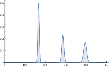
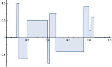
Figure 1: Functions to generate the first principal component vector $\bm{p}_{1}$.

The eigenvalues $\nu_{1},\dots,\nu_{p}$ of $A$ are determined by $\nu_{j}=\nu^{j}$, $j=1,\dots,p$, where $\nu\in\{0.85,0.6,0.35,0.1\}$. Under this setting, the ratio of the first eigenvalue of the covariance matrix $\Sigma_{0}$ to the second eigenvalue is $1+\nu^{2}$. We compare the average squared errors $\|\hat{\bm{\beta}}_{n}-\bm{\beta}^{0}\|/p$ in $l_{0}$-penalized estimator, $l_{1}$-penalized estimator and standard principal component analysis. The dimension $p$ of the stationary process is specified as $p=512$, while the number of the observation is specified as $n=256$. The penalty parameter $\lambda$ is taken as $\lambda_{0}=3\log(p)/n$ and $\lambda_{1}=(\log(p)/n)^{1/2}/3$. The numerical results reported in Table 1 are obtained over 1000 runs for the model (2.1) with i.i.d. innovations as centered Gaussian distribution and centered two-sided Weibull distribution with the shape parameter 0.5, respectively. Here, the covariance matrix of innovations is the identity matrix.

From Table 1, we see that the penalized principal component analysis performs better in terms of the loss than the standard principal component analysis for all cases. The penalized principal component analyses show similar performance, while the $l_{1}$-penalized estimator performs better in almost all cases in these simulations. The $l_{0}$-penalized estimators are prone to choose a small number of features while the $l_{1}$-penalized estimators balance the average squared error and the number of features.

Table 1: Comparison of principal component analyses; Peak refers to the three-peak function and Step refers to the step function. Loss refers to the average squared error and Size refers to the number of the estimated elements in the first principal component.

		$l_{0}$-penalized estimator	$l_{1}$-penalized estimator	Standard PCA
Gaussian
Vector	$\nu_{1}$	Loss (Size)	Loss (Size)	Loss
Peak	0.85	0.00304 (29.01)	0.00314 (47.92)	0.00422
	0.60	0.00350 (35.98)	0.00297 (49.43)	0.00513
	0.35	0.00331 (35.73)	0.00273 (49.42)	0.00505
	0.10	0.00324 (35.55)	0.00265 (49.42)	0.00501
Step	0.85	0.00410 (42.35)	0.00411 (47.17)	0.00424
	0.60	0.00362 (47.03)	0.00298 (51.58)	0.00513
	0.35	0.00342 (46.89)	0.00272 (51.51)	0.00505
	0.10	0.00336 (46.98)	0.00263 (51.41)	0.00501
Weibull
Vector	$\nu_{1}$	Loss (Size)	Loss (Size)	Loss
Peak	0.85	0.00566 ( 5.33)	0.00523 ( 9.07)	0.00607
	0.60	0.00523 (13.61)	0.00470 (19.69)	0.00595
	0.35	0.00508 (13.68)	0.00453 (19.37)	0.00584
	0.10	0.00500 (13.92)	0.00444 (19.86)	0.00578
Step	0.85	0.00587 (14.16)	0.00540 (20.08)	0.00603
	0.60	0.00522 (14.01)	0.00467 (20.04)	0.00595
	0.35	0.00506 (14.09)	0.00449 (19.98)	0.00582
	0.10	0.00505 (13.91)	0.00448 (19.73)	0.00583

6.2 Real data example.

We apply the sparse principal component analyses to the dataset of daily average temperatures in Kyoto, Japan. The data are from January 1, 1901 to December 31, 2020, which are over the last 120 years. We removed the temperature of February 29, if exists, to make each year have 365 days. To summarize, the dimension of the data is 365 and the sample size is 120.

In general, the temperature data appear to increase over the years. Assuming a linear trend in the temperature, we removed the trend from the original data and obtained detrended data, of which the partial data are shown in the left figure in Figure 2. The detrended temperature data appear to be stationary. We also plot the eigenvalues of the covariance matrix obtained from the detrended data. The spikiness condition in Assumption 2.3 seems to be satisfied. The sparsity feature of these data can be confirmed from the right figure in Figure 2.

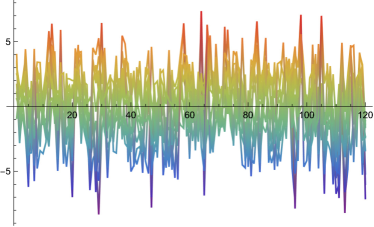
Figure 2: (Left) The detrended temperature data from April 20 to April 30 over 120 years. (Right) Eigenvalues of covariance matrix of the detrended temperature data.

The sparse principal component analyses and the standard principal component analysis are applied to the data. The penalty parameter $\lambda$ is taken as $\lambda_{0}=3\log(p)/n$ and $\lambda_{1}=(\log(p)/n)^{1/2}/3$ for $l_{0}$-penalty and $l_{1}$-penalty, respectively. The numerical results are obtained as Figure 3. The nonzero coefficients are shown in colors with rainbow plots. The estimates of large absolute value are in red while those of small absolute value are in blue. We can also find that the $l_{0}$-penalized estimate shows the smallest number of features in the first principal component, compared with other two methods, while the $l_{1}$-penalized estimate harmonize the standard principal components analysis with the $l_{0}$-penalized one.

The sparse principal component analyses explain the feature of the temperatures in Kyoto well. It is well known that the temperature in Kyoto is radically going up and down during February and March over years. Thus there is much more temperature variation during these months. This result matches the data provided by Japan Meteorological Agency. In summary, this feature is extracted by the sparse principal component analyses.

Figure 3: Plots for the estimated first principal components. From the top to bottom, plots are for the $l_{0}$-penalized estimate, the $l_{1}$-penalized estimate, and the standard one.

7 Proofs

In this section, we complement the rigorous proofs for the main results in Sections 3–5. First, we summarize some crucial technical results in Subsections 7.1 and 7.2 for $\alpha$-mixing Gaussian processes and $\beta$-mixing sub-Weibull processes, respectively. The proofs for technical results in Subsection 7.1 can be found in Subsection 7.3, while the proofs for technical results in Subsection 7.2 can be found in Subsection 7.4. Subsection 7.5 offers the proofs for $l_{0}$-penalized estimators.

7.1 Technical results for Gaussian process.

We use the following concentration inequality, which is a modified form of the Hanson-Wright inequality.

Lemma 7.1.

Let $\bm{Y}\sim N(\bm{0},Q)$ be an $n$-dimensional normal random vector. Then, there exists a universal constant $c>0$ such that for any $\eta>0$,

$$P\left(\frac{1}{n}\left|\|\bm{Y}\|_{2}^{2}-E[\|\bm{Y}\|_{2}^{2}]\right|>\eta\|Q\|_{2}\right)\leq 2\exp\left(-cn\min\{\eta,\eta^{2}\}\right).$$

See Rudelson and Vershynin (2013), Basu and Michailidis (2015), and Wong et al. (2020) for the detail of this inequality.

The next lemma guarantees that the empirical risk $R_{n}(\cdot)$ is also strictly convex on $\mathcal{B}$ with large probability.

Lemma 7.2.

Suppose that the same assumptions as Proposition 2.1 and Assumption 3.1 hold. Then, for every $0<\xi_{n}<\tau_{n}$, where

$$\tau_{n}:=\frac{\sigma-3\eta}{\sum_{l=0}^{n}\rho(l)\phi_{\max}},$$

and for every unit vector $\bm{v}\in\mathbb{R}^{p}$, it holds that

$$P\left(|\bm{v}^{\top}W_{n}\bm{v}|>\xi_{n}\sum_{l=0}^{n}\rho(l)\phi_{\max}\right)\leq 2\exp(-cn\min(\xi_{n},\xi_{n}^{2})),$$

which implies that

$$P(\bm{v}^{\top}\ddot{R}_{n}(\bm{\beta})\bm{v}>0)\geq 1-2\exp(-cn\min(\xi_{n},\xi_{n}^{2})),\quad\bm{\beta}\in\mathcal{B},$$

with some universal constant $c>0$.

For $\alpha$-mixing Gaussian processes, by Lemma 7.2, we find that for any convex penalty function ${\rm pen}(\cdot)$, $R_{n}(\cdot)+\lambda\,{\rm pen}(\cdot)$ is still asymptotically strictly convex on $\mathcal{B}$, which follows from the fact that the conical combination of convex functions is also convex. This also implies that $\hat{\bm{\beta}}_{n}^{1}$ is a unique solution to the optimization problem $i.e.$, the Lasso-type PCA estimator is well-defined with large probability.

We establish the oracle inequality for the estimator $\hat{\bm{\beta}}_{n}^{1}$. To do this, we should evaluate the difference between the empirical risk and theoretical risk, which is achieved by the following lemma.

Lemma 7.3.

Let $b>0$ be a free parameter and $\tilde{c}>0$ be a constant. Define that

$$\zeta_{n}:=\sqrt{\frac{(b+1)\log p^{2}}{\tilde{c}n}}.$$

Under the Assumptions 2.3, 3.1 and the same assumption as Proposition 2.1, for every $n$ satisfying $\log p/n\leq 1$, it holds that

$$P\left(\|W_{n}\|_{\max}\leq\zeta_{n}\sum_{l=0}^{n}\rho(l)\phi_{\max}\right)\geq 1-\exp(-b\log p^{2}),$$

where $W_{n}=\hat{\Sigma}_{n}-\Sigma_{0}$.

7.2 Technical results for sub-Weibull process.

To derive the oracle inequality for the $\beta$-mixing sub-Weibull process, we use the following concentration inequality, which is established by Merlevède et al. (2011).

Lemma 7.4.

Let $\{X_{t}\}_{t\in\mathbb{Z}}$ be an $\mathbb{R}$-valued zero mean strictly stationary process, which satisfies that

$$\beta(n)\leq 2\exp(-cn^{\gamma_{1}}),$$

and

$$\|X_{t}\|_{\psi_{\gamma_{2}}}\leq K,\quad\forall t\in\mathbb{Z},$$

for constants $c,\gamma_{1},\gamma_{2},\ K>0$. Let $\gamma$ be

$$\gamma:=\left(\frac{1}{\gamma_{1}}+\frac{1}{\gamma_{2}}\right)^{-1}<1.$$

Then, for every $n>4$ and $\epsilon>1/n$, it holds that

$$P\left(\left|\frac{1}{n}\sum_{t=1}^{n}X_{t}\right|>\epsilon\right) \leq n\exp\left(-\frac{(\epsilon n)^{\gamma}}{K^{\gamma}C_{1}}\right)+\exp\left(-\frac{\epsilon^{2}n}{K^{2}C_{2}}\right),$$

where $C_{1}$ and $C_{2}$ are constants depending only on $\gamma_{1},\gamma_{2}$ and $c$.

Using Lemma 7.4, we obtain the following result which is corresponding to the Lemma 7.2 for Gaussian case.

Lemma 7.5.

Suppose that the same assumptions as Proposition 2.1 and Assumption 4.2 hold. Then, for every $\xi_{n}$ such that

$$\frac{K_{2}C_{1}^{1/\gamma}(\log n)^{1/\gamma}}{n}<\xi_{n}<\sigma-3\eta,$$

where

$$K_{2}:=2^{2/\gamma_{2}}K^{2}$$

and for every unit vector $\bm{v}\in\mathbb{R}^{p}$, it holds that

$$P\left(|\bm{v}^{\top}W_{n}\bm{v}|>\xi_{n}\right)\leq 2n\exp\left(-\frac{(\xi_{n}n)^{\gamma}}{K_{2}^{\gamma}C_{1}}\right)+2\exp\left(-\frac{\xi_{n}^{2}n}{K_{2}^{2}C_{1}}\right),$$

where $C_{1}$ and $C_{2}$ are constants depending only on $c,\ \gamma_{1},\ \gamma_{2}$ described in Assumption 4.2. Especially, it holds that

$$P(\bm{v}^{\top}\ddot{R}_{n}(\bm{\beta})\bm{v}>0)\geq 1-2n\exp\left(-\frac{(\xi_{n}n)^{\gamma}}{K_{2}^{\gamma}C_{1}}\right)-2\exp\left(-\frac{\xi_{n}^{2}n}{K_{2}^{2}C_{2}}\right),\quad\bm{\beta}\in\mathcal{B}.$$

Note that if we take $\xi_{n}$ as

$$\xi_{n}=\frac{K_{2}C_{2}^{1/\gamma}(\log n)^{1/\gamma}}{n^{1-\alpha}},\quad\alpha\in(0,1/2),$$

for sufficiently large $n$, then, it holds that

$$P\left(|\bm{v}^{\top}W_{n}\bm{v}|>\xi_{n}\right)\to 0,\quad\text{as $n\to\infty$},$$

which implies that

$$P(\bm{v}^{\top}\ddot{R}_{n}(\bm{\beta})\bm{v}>0)\to 1,\quad\bm{\beta}\in\mathcal{B}.$$

Therefore, we conclude that for $\beta$-mixing sub-Weibull processes, $R_{n}(\cdot)+\lambda\,{\rm pen}(\cdot)$ is also asymptotically strictly convex on $\mathcal{B}$ with large probability for any convex penalty function ${\rm pen}(\cdot)$. As for the bound for $\|W_{n}\|_{\max}$, we have the following lemma.

Lemma 7.6.

Suppose that Assumptions 2.3 and 4.2 hold. For every $\zeta_{n}$ satisfying

$$\zeta_{n}>\max\left\{\frac{K_{2}C_{1}^{1/\gamma}(\log np^{2}+2\tilde{b}\log p)^{1/\gamma}}{n},K_{2}\sqrt{\frac{2C_{2}(\tilde{b}+1)\log p}{n}}\right\},$$

where $\tilde{b}>0$ is a free parameter, it holds that

$$P\left(\|W_{n}\|_{\max}\leq\zeta_{n}\right)\geq 1-2\exp(-\tilde{b}\log p^{2}).$$

7.3 Proofs for Subsection 7.1 and Section 3.

In this subsection, we provide proofs for main results and technical results for Lasso-type estimator for $\alpha$-mixing Gaussian process.

• Noting that

  $$\ddot{R}_{n}(\bm{\beta})=\ddot{R}(\bm{\beta})-(\hat{\Sigma}_{n}-\Sigma_{0}),$$

  we have that for every unit vector $\bm{v}\in\mathbb{R}^{p}$,

  $$\bm{v}^{\top}\ddot{R}_{n}(\bm{\beta})\bm{v} = \bm{v}^{\top}\ddot{R}_{n}(\bm{\beta})\bm{v}-\bm{v}^{\top}W_{n}\bm{v}$$

  $$\geq 2(\sigma-3\eta)-\bm{v}^{\top}W_{n}\bm{v},$$

  where $W_{n}:=\hat{\Sigma}_{n}-\Sigma_{0}$. Therefore, it suffices to evaluate the probability that $P(\bm{v}^{\top}W_{n}\bm{v}>\eta_{n})$ for some $\eta_{n}<\sigma-3\eta$. Put $\bm{X}_{(n)}=(\bm{X}_{1},\ldots,\bm{X}_{n})$. It follows from the stationarity of $\{\bm{X}_{t}\}_{t\in\mathbb{Z}}$ that

  $$\hat{\Sigma}_{n}=\frac{1}{n}\bm{X}_{(n)}\bm{X}_{(n)}^{\top},\quad\Sigma_{0}=\frac{1}{n}E[\bm{X}_{(n)}\bm{X}_{(n)}^{\top}],$$

  which implies that

  $$\bm{v}^{\top}W_{n}\bm{v} = \frac{1}{n}\bm{v}^{\top}(\bm{X}_{(n)}\bm{X}_{(n)}^{\top}-E[\bm{X}_{(n)}\bm{X}_{(n)}^{\top}])\bm{v}$$

  $$= \frac{1}{n}(\|\bm{X}_{(n)}^{\top}\bm{v}\|_{2}^{2}-E[\|\bm{X}_{(n)}^{\top}\bm{v}\|_{2}^{2}]).$$

  Let $Q_{n}$ be the covariance matrix of the random variable $\bm{X}_{(n)}^{\top}\bm{v}$. By the simple calculation, we can find that

  $$Q_{n}=\left(\begin{array}[]{ccc}\bm{v}^{\top}E[\bm{X}_{1}\bm{X}_{1}^{\top}]\bm{v}&\cdots&\bm{v}^{\top}E[\bm{X}_{1}\bm{X}_{n}^{\top}]\bm{v}\\ \vdots&\ddots&\vdots\\ \bm{v}^{\top}E[\bm{X}_{n}\bm{X}_{1}^{\top}]\bm{v}&\cdots&\bm{v}^{\top}E[\bm{X}_{n}\bm{X}_{n}^{\top}]\bm{v}\end{array}\right).$$

  Noting that $\{\bm{X}_{t}\}_{t\in\mathbb{Z}}$ is a centered Gaussian time series, we have that $\bm{X}_{(n)}^{\top}\bm{v}\sim N(\bm{0},Q_{n})$. We can apply Lemma 7.1 to $\bm{X}_{(n)}^{\top}\bm{v}$ to deduce that for every $\xi>0$,

  $$P\left(\frac{1}{n}\left|\|\bm{X}_{(n)}^{\top}\bm{v}\|_{2}^{2}-E[\|\bm{X}_{(n)}^{\top}\bm{v}\|_{2}^{2}]\right|>\xi\|Q_{n}\|_{2}\right)\leq 2\exp(-cn\min\{\xi,\xi^{2}\}),$$

  where $c>0$ is a universal constant. Noting that the $\alpha$-mixing Gaussian time series $\{\bm{X}_{t}\}_{t\in\mathbb{Z}}$ is also $\rho$-mixing, we have

  $$\|Q_{n}\|_{2}\leq\sum_{l=0}^{n}\rho(l)\|\Sigma_{0}\|_{2}=\sum_{l=0}^{n}\rho(l)\phi_{\max}.$$

  We therefore obtain that

  $$P\left(\frac{1}{n}\left|\|\bm{X}_{(n)}^{\top}\bm{v}\|_{2}^{2}-E[\|\bm{X}_{(n)}^{\top}\bm{v}\|_{2}^{2}]\right|>\xi\sum_{l=0}^{n}\rho(l)\phi_{\max}\right)\leq 2\exp(-cn\min\{\xi,\xi^{2}\}).$$

  Especially, we can take a sequence $\xi_{n}$ satisfying that

  $$0<\xi_{n}<\frac{\sigma-3\eta}{\sum_{l=0}^{n}\rho(l)\phi_{\max}},$$

  which concludes the lemma.

• For every $i,j\in\{1,\ldots,p\}$, it holds that

  $$W_{nij}=\bm{e}_{i}^{\top}W_{n}\bm{e}_{j},$$

  where $\bm{e}_{k},\ k=1,\ldots,p$ is the $k$-th canonical basis of $\mathbb{R}^{p}$. Since

  $$W_{n}=\hat{\Sigma}_{n}-\Sigma_{0}=\frac{1}{n}(\bm{X}_{(n)}\bm{X}_{(n)}^{\top}-E[\bm{X}_{(n)}\bm{X}_{(n)}^{\top}]),$$

  it holds that

  $$W_{nij}=\frac{1}{n}\left(\bm{e}_{i}^{\top}\bm{X}_{(n)}\bm{X}_{(n)}^{\top}\bm{e}_{j}-E[\bm{e}_{i}^{\top}\bm{X}_{(n)}\bm{X}_{(n)}^{\top}\bm{e}_{j}]\right).$$

  Putting $\bm{Y}_{k}=\bm{X}_{(n)}^{\top}\bm{e}_{k},\ k=1,\ldots,p$, we can rewrite that

  $$W_{nij}=\frac{1}{n}\left(\bm{Y}_{i}^{\top}\bm{Y}_{j}-E[\bm{Y}_{i}^{\top}\bm{Y}_{j}]\right).$$

  Note that

  $$\bm{Y}_{i}^{\top}\bm{Y}_{j}-E[\bm{Y}_{i}^{\top}\bm{Y}_{j}] = \frac{1}{2}\left\{(\|\bm{Y}_{i}+\bm{Y}_{j}\|_{2}^{2}-E[\|\bm{Y}_{i}+\bm{Y}_{j}\|_{2}^{2}])\right.$$

  $$\left.-(\|\bm{Y}_{i}\|_{2}^{2}-E[\|\bm{Y}_{i}\|_{2}^{2}])-(\|\bm{Y}_{j}\|_{2}^{2}-E[\|\bm{Y}_{j}\|_{2}^{2}])\right\}.$$

  We then find that

  $$|W_{nij}| = \frac{1}{n}\left|\bm{Y}_{i}^{\top}\bm{Y}_{j}-E[\bm{Y}_{i}^{\top}\bm{Y}_{j}]\right|$$

  $$\leq \frac{1}{2n}\left|(\|\bm{Y}_{i}+\bm{Y}_{j}\|_{2}^{2}-E[\|\bm{Y}_{i}+\bm{Y}_{j}\|_{2}^{2}]\right|$$

  $$+\frac{1}{2n}\left|\|\bm{Y}_{i}\|_{2}^{2}-E[\|\bm{Y}_{i}\|_{2}^{2}]\right|+\frac{1}{2n}\left|\|\bm{Y}_{j}\|_{2}^{2}-E[\|\bm{Y}_{j}\|_{2}^{2}]\right|.$$

  Also, $\bm{Y}_{i},\ \bm{Y}_{j},\ \bm{Y}_{i}+\bm{Y}_{j}$ are centered Gaussian random variables. Denote the covariance matrices of them by $\Sigma_{Y_{i}},\ \Sigma_{Y_{j}},$ and $\Sigma_{Y_{i}+Y_{j}}$, respectively. Then, the following inequalities directly follow from Lemma 7.1 that for every $\zeta>0$, there exists a universal constant $\tilde{c}>0$ such that,

  $$P\left(\frac{1}{n}\left|\|\bm{Y}_{i}\|_{2}^{2}-E[\|\bm{Y}_{i}\|_{2}^{2}]\right|>\zeta\|\Sigma_{Y_{i}}\|_{2}\right)\leq 2\exp(-\tilde{c}n\min\{\zeta,\zeta^{2}\}),$$ (7.1)

  $$P\left(\frac{1}{n}\left|\|\bm{Y}_{j}\|_{2}^{2}-E[\|\bm{Y}_{j}\|_{2}^{2}]\right|>\zeta\|\Sigma_{Y_{j}}\|_{2}\right)\leq 2\exp(-\tilde{c}n\min\{\zeta,\zeta^{2}\}),$$ (7.2)

  and

  $$P\left(\frac{1}{n}\left|\|\bm{Y}_{i}+\bm{Y}_{j}\|_{2}^{2}-E[\|\bm{Y}_{i}+\bm{Y}_{j}\|_{2}^{2}]\right|>\zeta\|\Sigma_{Y_{i}+Y_{j}}\|_{2}\right)\leq 2\exp(-\tilde{c}n\min\{\zeta,\zeta^{2}\}).$$

  After some tedious computation, we have

  $$\|\Sigma_{Y_{i}+Y_{j}}\|_{2}\leq\frac{\|\Sigma_{Y_{i}}\|_{2}+\|\Sigma_{Y_{j}}\|_{2}}{2}.$$

  Therefore, we have that

  $$P\left(\frac{1}{n}\left|\|\bm{Y}_{i}+\bm{Y}_{j}\|_{2}^{2}-E[\|\bm{Y}_{i}+\bm{Y}_{j}\|_{2}^{2}]\right|\right. > \left.\frac{\zeta(\|\Sigma_{Y_{i}}\|_{2}+\|\Sigma_{Y_{j}})\|_{2}}{2}\right)$$ (7.3)

  $$\leq 2\exp(-\tilde{c}n\min\{\zeta,\zeta^{2}\}).$$

  The inequalities (7.1)–(7.3) imply that for every $\zeta>0$, there exists a constant $\tilde{c}$ such that

  $$P(|W_{nij}|>\zeta(\|\Sigma_{Y_{i}}\|_{2}+\|\Sigma_{Y_{i}}\|_{2}))\leq 6\exp(-\tilde{c}n\min\{\zeta,\zeta^{2}\}).$$

  Let $b>0$ be a free parameter. We take $\zeta$ as

  $$\zeta:=\zeta_{n}=\sqrt{\frac{(b+1)\log p^{2}}{\tilde{c}n}}.$$

  Then, for every $n$ such that $\zeta_{n}^{2}<\zeta_{n}$, it holds that

  $$P\left(\|W_{n}\|_{\max}>4\zeta\sum_{l=0}^{n}\rho(l)\phi_{\max}\right) \leq P\left(\|W_{n}\|_{\max}>\max_{i,j}\zeta(\|\Sigma_{Y_{i}}\|_{2}+\|\Sigma_{Y_{j}}\|_{2})\right)$$

  $$= P\left(\max_{i,j}|\bm{e}_{i}^{\top}W_{n}\bm{e}_{j}|>\max_{i,j}\zeta(\|\Sigma_{Y_{i}}\|_{2}+\|\Sigma_{Y_{j}}\|_{2})\right)$$

  $$\leq \sum_{i,j}P\left(|\bm{e}_{i}^{\top}W_{n}\bm{e}_{j}|>\zeta(\|\Sigma_{Y_{i}}\|_{2}+\|\Sigma_{Y_{j}}\|_{2})\right)$$

  $$\leq 6p^{2}\exp(-\tilde{c}n\min\{\zeta,\zeta^{2}\})$$

  $$= 6\exp\left(\log p^{2}-\tilde{c}n\frac{(b+1)\log p^{2}}{\tilde{c}n}\right)$$

  $$= 6\exp(-b\log p^{2}),$$

  which completes the proof.

• Let $\eta_{n}$ and $\gamma_{n}$ be

  $$\eta_{n}=\xi_{n}\sum_{l=0}^{n}\rho(l)\phi_{\max},$$

  and

  $$\gamma_{n}=\zeta_{n}\sum_{l=0}^{n}\rho(l)\phi_{\max},$$

  respectively. Under the constraints $\xi_{n}<\tau_{n}:=\frac{\sigma-3\eta}{\sum_{l=0}^{n}\rho(l)\phi_{\max}}$, it suffices to show the inequality

  $$\|\hat{\bm{\beta}}_{n}^{1}-\bm{\beta}^{0}\|_{1}\leq\frac{2(C+1)^{2}\lambda_{1}s_{0}}{\sigma-3\eta-\eta_{n}}$$ (7.4)

  on the event

  $$\{\|W_{n}\|_{\max}\leq\gamma_{n}\}\cap\{|\bm{v}^{\top}W_{n}\bm{v}|\leq\eta_{n}\}$$

  for

  $$\bm{v}=\frac{\hat{\bm{\beta}}^{1}_{n}-\bm{\beta}^{0}}{\|\hat{\bm{\beta}}^{1}_{n}-\bm{\beta}^{0}\|_{2}}.$$

  Following Lemma 7.1 of van de Geer (2016), it holds that

  $$-\dot{R}_{n}(\hat{\bm{\beta}}_{n}^{1})^{\top}(\bm{\beta}^{0}-\hat{\bm{\beta}}_{n}^{1})\leq\lambda_{1}\|\bm{\beta}^{0}\|_{1}-\lambda_{1}\|\hat{\bm{\beta}}_{n}^{1}\|_{1}.$$ (7.5)

  Moreover, it follows from Proposition 2.1 and the Taylor expansion that

  $$R(\bm{\beta}^{0})-R(\hat{\bm{\beta}}_{n}^{1})-\dot{R}(\hat{\bm{\beta}}_{n}^{1})^{\top}(\bm{\beta}^{0}-\hat{\bm{\beta}}_{n}^{1})\geq(\sigma-3\eta)\|\bm{\beta}^{0}-\hat{\bm{\beta}}^{1}_{n}\|_{2}^{2}\geq 0.$$ (7.6)

  Combining (7.5) and (7.6), we have that

  $$R(\hat{\bm{\beta}}^{1}_{n})-R(\bm{\beta}^{0})+\lambda_{1}\|\hat{\bm{\beta}}^{1}_{n}\|_{1}\leq\bigl{(}\dot{R}_{n}(\hat{\bm{\beta}}^{1}_{n})-\dot{R}(\hat{\bm{\beta}}^{1}_{n})\bigr{)}^{\top}(\bm{\beta}^{0}-\hat{\bm{\beta}}^{1}_{n})+\lambda_{1}\|\bm{\beta}^{0}\|_{1}.$$ (7.7)

  Noting that

  $$\dot{R}_{n}(\hat{\bm{\beta}}^{1}_{n})-\dot{R}(\hat{\bm{\beta}}^{1}_{n})=-W_{n}\hat{\bm{\beta}}^{1}_{n},$$

  we have, on the event $\{|\bm{v}^{\top}W_{n}\bm{v}|\leq\eta_{n}\}$,

  $$\bigl{(}\dot{R}_{n}(\hat{\bm{\beta}}^{1}_{n})-\dot{R}(\hat{\bm{\beta}}^{1}_{n})\bigr{)}^{\top}(\bm{\beta}^{0}-\hat{\bm{\beta}}^{1}_{n}) =-\hat{\bm{\beta}}_{n}^{1\top}W_{n}(\bm{\beta}^{0}-\hat{\bm{\beta}}^{1}_{n})$$

  $$=(\hat{\bm{\beta}}^{1}_{n}-\bm{\beta}^{0})^{\top}W_{n}(\hat{\bm{\beta}}^{1}_{n}-\bm{\beta}^{0})+\bm{\beta}^{0\top}W_{n}(\hat{\bm{\beta}}^{1}_{n}-\bm{\beta}^{0})$$

  $$\leq\eta_{n}\|\hat{\bm{\beta}}^{1}_{n}-\bm{\beta}^{0}\|_{2}^{2}+\|W_{n}\|_{\max}\|\bm{\beta}^{0}\|_{1}\|\hat{\bm{\beta}}^{1}_{n}-\bm{\beta}^{0}\|_{1}.$$ (7.8)

  Since $\bm{\beta}^{0}$ satisfies that $\dot{R}(\bm{\beta}^{0})=\bm{0}$, it follows from Proposition 2.1 and the Taylor expansion that

  $$R(\hat{\bm{\beta}}^{1}_{n})-R(\bm{\beta}^{0})\geq(\sigma-3\eta)\|\hat{\bm{\beta}}^{1}_{n}-\bm{\beta}^{0}\|_{2}^{2},$$

  which implies

  $$R(\hat{\bm{\beta}}^{1}_{n})-R(\bm{\beta}^{0})+\lambda_{1}\|\hat{\bm{\beta}}_{n}^{1}\|\geq(\sigma-3\eta)\|\hat{\bm{\beta}}^{1}_{n}-\bm{\beta}^{0}\|_{2}^{2}+\lambda_{1}\|\hat{\bm{\beta}}_{n}^{1}\|.$$ (7.9)

  Therefore, by (7.9), (7.7) and (7.8), we find that, on the event $\{\|W_{n}\|_{\max}\leq\gamma_{n}\}$,

  $$(\sigma-3\eta)\|\hat{\bm{\beta}}^{1}_{n}-\bm{\beta}^{0}\|_{2}^{2}+\lambda_{1}\|\hat{\bm{\beta}}^{1}_{n}\|_{1}\leq\eta_{n}\|\hat{\bm{\beta}}^{1}_{n}-\bm{\beta}^{0}\|_{2}^{2}+\gamma_{n}\|\bm{\beta}^{0}\|_{1}\|\hat{\bm{\beta}}^{1}_{n}-\bm{\beta}^{0}\|_{1}+\lambda_{1}\|\bm{\beta}^{0}\|_{1},$$

  and thus,

  $$(\sigma-3\eta-\eta_{n})\|\hat{\bm{\beta}}^{1}_{n}-\bm{\beta}^{0}\|_{2}^{2}\leq\gamma_{n}\|\bm{\beta}^{0}\|_{1}\|\hat{\bm{\beta}}^{1}_{n}-\bm{\beta}^{0}\|_{1}+\lambda_{1}\|\bm{\beta}^{0}\|_{1}-\lambda_{1}\|\hat{\bm{\beta}}^{1}_{n}\|_{1}.$$ (7.10)

  The right-hand side of (7.10) can be bounded as follows.

  $$\gamma_{n}\|\bm{\beta}^{0}\|_{1}\|\hat{\bm{\beta}}^{1}_{n}-\bm{\beta}^{0}\|_{1}+\lambda_{1}\|\bm{\beta}^{0}\|_{1}-\lambda_{1}\|\hat{\bm{\beta}}^{1}_{n}\|_{1}$$

  $$=\quad \gamma_{n}\|\bm{\beta}^{0}\|_{1}\|\hat{\bm{\beta}}^{1}_{nS}-\bm{\beta}^{0}_{S}\|_{1}+\gamma_{n}\|\bm{\beta}^{0}\|_{1}\|\hat{\bm{\beta}}^{1}_{nS^{c}}-\bm{\beta}^{0}_{S^{c}}\|_{1}$$

  $$+\lambda_{1}\|\bm{\beta}^{0}_{S}\|_{1}+\lambda_{1}\|\bm{\beta}^{0}_{S^{c}}\|_{1}-\lambda_{1}\|\hat{\bm{\beta}}^{1}_{nS}\|_{1}-\lambda_{1}\|\hat{\bm{\beta}}^{1}_{nS^{c}}\|_{1}$$

  $$\leq\quad (\lambda_{1}+\gamma_{n}\|\bm{\beta}^{0}\|_{1})\|\hat{\bm{\beta}}^{1}_{nS}-\bm{\beta}^{0}_{S}\|_{1}-(\lambda_{1}-\gamma_{n}\|\bm{\beta}^{0}\|_{1})\|\hat{\bm{\beta}}^{1}_{nS^{c}}-\bm{\beta}^{0}_{S^{c}}\|_{1}.$$ (7.11)

  Since $\eta_{n}<\sigma-3\eta$, we see that the left-hand side of (7.10) is positive. Hence, we have that

  $$0<(\lambda_{1}+\gamma_{n}\|\bm{\beta}^{0}\|_{1})\|\hat{\bm{\beta}}^{1}_{nS}-\bm{\beta}^{0}_{S}\|_{1}-(\lambda_{1}-\gamma_{n}\|\bm{\beta}^{0}\|_{1})\|\hat{\bm{\beta}}^{1}_{nS^{c}}-\bm{\beta}^{0}_{S^{c}}\|_{1}.$$ (7.12)

  Now let $\Delta:=\hat{\bm{\beta}}^{1}_{n}-\bm{\beta}^{0}$. By (7.12), we then find that

  $$\|\Delta_{S^{c}}\|_{1}\leq\frac{\lambda_{1}+\gamma_{n}\|\bm{\beta}^{0}\|_{1}}{\lambda_{1}-\gamma_{n}\|\bm{\beta}^{0}\|_{1}}\|\Delta_{S}\|_{1}\leq C\|\Delta_{S}\|_{1}.$$

  Consequently, we have that

  $$\|\Delta\|_{1}\leq(C+1)\|\Delta_{S}\|_{1},$$

  In view of $\|\Delta_{S}\|_{1}\leq\sqrt{s_{0}}\|\Delta\|_{2}$, we then obtain

  $$\frac{\|\Delta\|_{1}}{(C+1)\sqrt{s_{0}}}\leq\frac{\|\Delta_{S}\|_{1}}{\sqrt{s_{0}}}\leq\|\Delta\|_{2},$$

  which implies that

  $$(\sigma-3\eta-\eta_{n})\|\Delta\|_{2}^{2}\geq\frac{\sigma-3\eta-\eta_{n}}{(C+1)^{2}s_{0}}\|\Delta\|_{1}^{2}.$$

  Using (7.10) and (7.11), we finally obtain that

  $$\frac{\sigma-3\eta-\eta_{n}}{(C+1)^{2}s_{0}}\|\Delta\|_{1}^{2} \leq (\lambda_{1}+\gamma_{n}\|\bm{\beta}^{0}\|_{1})\|\Delta_{S}\|_{1}-(\lambda_{1}-\gamma_{n}\|\bm{\beta}^{0}\|_{1})\|\Delta_{S^{c}}\|_{1}$$

  $$\leq (\lambda_{1}+\gamma_{n}\|\bm{\beta}^{0}\|_{1})\|\Delta_{S}\|_{1}+(\lambda_{1}-\gamma_{n}\|\bm{\beta}^{0}\|_{1})\|\Delta_{S^{c}}\|_{1}$$

  $$\leq (\lambda_{1}+\gamma_{n}\|\bm{\beta}^{0}\|_{1})\|\Delta\|_{1}+(\lambda_{1}-\gamma_{n}\|\bm{\beta}^{0}\|_{1})\|\Delta\|_{1}$$

  $$= 2\lambda_{1}\|\Delta\|_{1},$$

  which ends the proof of (7.4).

7.4 Proofs for Subsection 7.2 and Section 4.

In this subsection, we provide proofs for main results and technical results for Lasso-type estimator for $\beta$-mixing sub-Weibull process.

• For every $\bm{v}\in\mathbb{S}^{p-1}$, it holds that

  $$\bm{v}^{\top}W_{n}\bm{v}=\frac{1}{n}(\|\bm{X}_{(n)}^{\top}\bm{v}\|_{2}^{2}-E[\|\bm{X}_{(n)}^{\top}\bm{v}\|_{2}^{2}]).$$

  Define the process $\{Z_{t}(\bm{v})\}_{t\in\mathbb{Z}}$ by

  $$Z_{t}(\bm{v})=|\bm{v}^{\top}\bm{X}_{t}|^{2}-E[|\bm{v}^{\top}\bm{X}_{t}|^{2}].$$

  Then, we have that

  $$\|\bm{X}_{(n)}^{\top}\bm{v}\|_{2}^{2}-E[\|\bm{X}_{(n)}^{\top}\bm{v}\|_{2}^{2}]=\sum_{t=1}^{n}Z_{t}(\bm{v}).$$

  Since $\{\bm{X}_{t}\}_{t\in\mathbb{Z}}$ is the sub-Weibull $(\gamma_{2})$, the process $\{Z_{t}(\bm{v})\}_{t\in\mathbb{Z}}$ is the sub-Weibull $(\gamma_{2}/2)$. Therefore, it follows from Lemma 7.4 that

  $$P(|\bm{v}^{\top}W_{n}\bm{v}|>\xi_{n}) = P\left(\left|\frac{1}{n}\sum_{t=1}^{n}Z_{t}(\bm{v})\right|>\xi_{n}\right)$$

  $$\leq 2n\exp\left(-\frac{(\xi_{n}n)^{\gamma}}{K_{2}C_{1}}\right)+\exp\left(-\frac{\xi_{n}^{2}n}{K_{2}^{2}C_{2}}\right),$$

  which completes the proof.

• As well as Proof of Lemma 7.3, we can find that

  $$|W_{nij}| \leq \frac{1}{2n}\left|(\|\bm{Y}_{i}+\bm{Y}_{j}\|_{2}^{2}-E[\|\bm{Y}_{i}+\bm{Y}_{j}\|_{2}^{2}]\right|$$

  $$+\frac{1}{2n}\left|\|\bm{Y}_{i}\|_{2}^{2}-E[\|\bm{Y}_{i}\|_{2}^{2}]\right|+\frac{1}{2n}\left|\|\bm{Y}_{j}\|_{2}^{2}-E[\|\bm{Y}_{j}\|_{2}^{2}]\right|,$$

  where $\bm{Y}_{k}=\bm{X}_{(n)}^{\top}\bm{e}_{k},\ k=1,\ldots,p$. Note that

  $$\|\bm{Y}_{i}\|_{2}^{2}=\sum_{t=1}^{n}X_{i,t}^{2},\quad\|\bm{Y}_{i}+\bm{Y}_{j}\|_{2}^{2}=\sum_{t=1}^{n}(X_{i,t}^{2}+X_{j,t}^{2}),\quad i,j=1,\ldots,p,$$

  where $X_{i,t}$ is the $i$-th component of $\bm{X}_{t}$. Since the process $\{\bm{X}_{t}\}_{t\in\mathbb{Z}}$ is sub-Weibull $(\gamma_{2})$, it follows that $\{X_{i,t}^{2}\}_{t\in\mathbb{Z}}$ is sub-Weibull $(\gamma_{2}/2)$. Therefore, we can apply Lemma 7.5 to deduce the conclusion.

• It suffices to show the inequality on the event

  $$\{\|W_{n}\|_{\max}\leq\zeta_{n}\}\cap\{\bm{v}^{\top}W_{n}\bm{v}\leq\xi_{n}\},$$

  where

  $$\bm{v}=\frac{\hat{\bm{\beta}}_{n}^{1}-\bm{\beta}^{0}}{\|\hat{\bm{\beta}}_{n}^{1}-\bm{\beta}^{0}\|_{2}}.$$

  The remaining part of the proof is similar to the proof of Theorem 3.1.

7.5 $l_{0}$-penalized estimator for $\alpha$-mixing Gaussian process.

In this subsection, we prove main results for the $l_{0}$-penalized estimator for $\alpha$-mixing process.

Lemma 7.7.

Suppose that Assumptions 2.3 and 3.1 hold. Let $\zeta_{n}$ be

$$\tilde{\zeta}_{n}=\sqrt{\frac{(b+4\tilde{s})\log p}{cn}},$$

where $b>0$ is a free parameter and $c>0$ is a constant. For every $p>6$ and $n$ such that $\tilde{\zeta}_{n}^{2}<\tilde{\zeta}_{n}$, it holds that

$$P\left(\sup_{v\in\mathcal{B}(2\tilde{s})\cap\mathbb{S}^{p-1}}|\bm{v}^{\top}W_{n}\bm{v}|>\tilde{\zeta}_{n}\sum_{l=0}^{n}\rho(l)\phi_{\max}\right)\leq\exp\left(-b\log p\right).$$

• First, we fix $\bm{v}\in\mathcal{B}_{0}(2\tilde{s})\cap\mathbb{S}^{p-1}$ arbitrarily. In view of the proof of Lemma 7.2, we have that

  $$|\bm{v}^{\top}W_{n}\bm{v}|=\frac{1}{n}\left|\|\bm{X}_{(n)}^{\top}\bm{v}\|_{2}^{2}-E[\|\bm{X}_{(n)}^{\top}\bm{v}\|_{2}^{2}]\right|.$$

  It follows from Lemma 7.1 that there exists a constant $c>0$ such that for every $\zeta>0$,

  $$P\left(\frac{1}{n}\left|\|\bm{X}_{(n)}^{\top}\bm{v}\|_{2}^{2}-E[\|\bm{X}_{(n)}^{\top}\bm{v}\|_{2}^{2}]\right|>\zeta\|Q_{n}\|_{2}\right)\leq 2\exp(-cn\min\{\zeta,\zeta^{2}\}),$$

  where $Q_{n}$ is the covariance matrix of $\bm{X}_{(n)}^{\top}\bm{v}$. Noting that

  $$\|Q_{n}\|_{2}\leq\sum_{l=0}^{n}\rho(l)\phi_{\max},$$

  we have

  $$P\left(\frac{1}{n}\left|\|\bm{X}_{(n)}^{\top}\bm{v}\|_{2}^{2}-E[\|\bm{X}_{(n)}^{\top}\bm{v}\|_{2}^{2}]\right|>\zeta\sum_{l=0}^{n}\rho(l)\phi_{\max}\right)\leq 2\exp(-cn\min\{\zeta,\zeta^{2}\}).$$

  Then, we take a union bound over $\mathcal{B}_{0}(2\tilde{s})\cap\mathbb{S}^{p-1}$. It is easy to see that we need

  $$\left(\begin{array}[]{c}p\\ 2\tilde{s}\\ \end{array}\right)6^{2\tilde{s}}$$

  points to cover the set $\mathcal{B}_{0}(2\tilde{s})\cap\mathbb{S}^{p-1}$ by balls with radius $1/2$. See $e.g.$, Chapter 4 of Vershynin (2018). We wright $\mathcal{N}_{1/2}$ for the set of centers of $1/2$-balls which covers $\mathcal{B}_{0}(2\tilde{s})\cap\mathbb{S}^{p-1}$. Then, it holds that

  $$P\left(\sup_{v\in\mathcal{B}_{0}(2\tilde{s})\cap\mathbb{S}^{p-1}}\frac{1}{n}\left|\|\bm{X}_{(n)}^{\top}\bm{v}\|_{2}^{2}-E[\|\bm{X}_{(n)}^{\top}\bm{v}\|_{2}^{2}]\right|>\zeta\sum_{l=0}^{n}\rho(l)\phi_{\max}\right)$$

  $$\leq \sum_{v\in\mathcal{N}_{1/2}}P\left(\frac{1}{n}\left|\|\bm{X}_{(n)}^{\top}\bm{v}\|_{2}^{2}-E[\|\bm{X}_{(n)}^{\top}\bm{v}\|_{2}^{2}]\right|>\zeta\sum_{l=0}^{n}\rho(l)\phi_{\max}\right)$$

  $$\leq \left(\begin{array}[]{c}p\\ 2\tilde{s}\\ \end{array}\right)6^{2\tilde{s}}2\exp(-cn\min\{\zeta,\zeta^{2}\})$$

  $$\leq (6p)^{2\tilde{s}}2\exp(-cn\min\{\zeta,\zeta^{2}\})$$

  $$= 2\exp\left(2\tilde{s}\log p+2\tilde{s}\log 6-cn\min\{\zeta,\zeta^{2}\}\right)$$

  $$\leq 2\exp\left(4\tilde{s}\log p-cn\min\{\zeta,\zeta^{2}\}\right)$$

  If we replace $\zeta$ with $\tilde{\zeta}_{n}$, then we obtain the conclusion.

• It suffices to show the inequality

  $$\|\hat{\bm{\beta}}^{0}_{n}-\bm{\beta}^{0}\|_{2}\leq\delta_{n}$$

  on the event

  $$\left\{\sup_{v\in\mathcal{B}_{0}(2\tilde{s})\cap\mathbb{S}^{p-1}}|\bm{v}^{\top}W_{n}\bm{v}|\leq\tilde{\gamma}_{n}\right\}.$$

  Note that $\hat{\bm{\beta}}^{0}_{n}-\bm{\beta}^{0}\in\mathcal{B}_{0}(2\tilde{s})$. Along the same lines as the proof of Theorem 3.1, we have the following analog to (7.9), (7.7) and (7.8) that

  $$(\sigma-3\eta)\|\hat{\bm{\beta}}^{0}_{n}-\bm{\beta}^{0}\|_{2}^{2}+\lambda_{0}\|\hat{\bm{\beta}}^{0}_{n}\|_{0} \leq R(\hat{\bm{\beta}}^{0}_{n})-R(\bm{\beta}^{0})+\lambda_{0}\|\hat{\bm{\beta}}^{0}_{n}\|_{0}$$

  $$\leq\bigl{(}\dot{R}_{n}(\hat{\bm{\beta}}^{0}_{n})-\dot{R}(\hat{\bm{\beta}}^{0}_{n})\bigr{)}^{\top}(\bm{\beta}^{0}-\hat{\bm{\beta}}^{0}_{n})+\lambda_{0}\|\bm{\beta}^{0}\|_{0}$$

  $$\leq\tilde{\gamma}_{n}\|\hat{\bm{\beta}}^{0}_{n}-\bm{\beta}^{0}\|_{2}^{2}+\bm{\beta}^{0\top}W_{n}(\hat{\bm{\beta}}^{0}_{n}-\bm{\beta}^{0})+\lambda_{0}\|\bm{\beta}^{0}\|_{0},$$

  and thus, it holds that

  $$(\sigma-3\eta-\tilde{\gamma}_{n})\|\hat{\bm{\beta}}^{0}_{n}-\bm{\beta}^{0}\|_{2}^{2} \leq|\bm{\beta}^{0\top}W_{n}(\hat{\bm{\beta}}_{n}^{0}-\bm{\beta}^{0})|+\lambda_{0}\|\bm{\beta}^{0}\|_{0}-\lambda_{0}\|\hat{\bm{\beta}}_{n}^{0}\|_{0}$$

  $$\leq\|W_{n}^{1/2}\bm{\beta}^{0}\|_{2}\|W_{n}^{1/2}(\hat{\bm{\beta}}_{n}^{0}-\bm{\beta}^{0})\|_{2}+\lambda_{0}\tilde{s}$$

  $$\leq\tilde{\gamma}_{n}\|\bm{\beta}^{0}\|_{2}\|\hat{\bm{\beta}}_{n}^{0}-\bm{\beta}^{0}\|_{2}+\lambda_{0}\tilde{s}.$$

  Noting that $\|\bm{\beta}^{0}\|_{2}=\phi_{\max}$, we reach the conclusion after solving the quadratic inequality with respect to $\|\hat{\bm{\beta}}^{0}_{n}-\bm{\beta}^{0}\|_{2}$.

References

- (1)
- Amini and Wainwright (2009) Amini, A. A. and Wainwright, M. J. (2009). High-dimensional analysis of semidefinite relaxations for sparse principal components. The Annals of Statistics 37 2877–2921.
- Anderson (1963) Anderson, T. W. (1963). Asymptotic theory for principal component analysis. The Annals of Mathematical Statistics 34 122–148.
- Basu and Michailidis (2015) Basu, S. and Michailidis, G. (2015). Regularized estimation in sparse high-dimensional time series models. The Annals of Statistics 43 1535–1567.
- Berthet and Rigollet (2013) Berthet, Q. and Rigollet, P. (2013). Optimal detection of sparse principal components in high dimension. The Annals of Statistics 41 1780–1815.
- Birnbaum et al. (2013) Birnbaum, A., Johnstone, I. M., Nadler, B., and Paul, D. (2013). Minimax bounds for sparse PCA with noisy high-dimensional data. The Annals of Statistics 41 1055–1084.
- Bühlmann and van de Geer (2011) Bühlmann, P. and van de Geer, S. (2011). Statistics for High-Dimensional Data: Methods, Theory and Applications. Springer.
- Cai et al. (2013) Cai, T. T., Ma, Z., and Wu, Y. (2013). Sparse PCA: Optimal rates and adaptive estimation. The Annals of Statistics 41 3074–3110.
- Cai and Zhou (2012) Cai, T. T. and Zhou, H. H. (2012). Optimal rates of convergence for sparse covariance matrix estimation. The Annals of Statistics 40 2389–2420.
- van de Geer (2016) van de Geer, S. A. (2016). Estimation and Testing under Sparsity. Springer.
- Jin et al. (2009) Jin, B., Wang, C., Miao, B., and Huang, M.-N. L. (2009). Limiting spectral distribution of large-dimensional sample covariance matrices generated by VARMA. Journal of Multivariate Analysis 100 2112–2125.
- Johnstone (2001) Johnstone, I. M. (2001). On the distribution of the largest eigenvalue in principal components analysis. The Annals of Statistics 29 295–327.
- Johnstone and Lu (2009) Johnstone, I. M. and Lu, A. Y. (2009). On consistency and sparsity for principal components analysis in high dimensions. Journal of the American Statistical Association 104 682–693.
- Jolliffe (2002) Jolliffe, I. T. (2002). Principal Component Analysis. Springer.
- Ma (2013) Ma, Z. (2013). Sparse principal component analysis and iterative thresholding. The Annals of Statistics 41 772–801.
- Merlevède et al. (2011) Merlevède, F., Peligrad, M., and Rio, E. (2011). A Bernstein type inequality and moderate deviations for weakly dependent sequences. Probability Theory and Related Fields 151 435–474.
- Paul and Johnstone (2012) Paul, D. and Johnstone, I. M. (2012). Augmented Sparse Principal Component Analysis for High Dimensional Data. , Technical Report. Available at arXiv:1202.1242v1.
- Pourahmadi (2013) Pourahmadi, M. (2013). High-Dimensional Covariance Estimation. John Wiley & Sons.
- Rudelson and Vershynin (2013) Rudelson, M. and Vershynin, R. (2013). Hanson-Wright inequality and sub-Gaussian concentration. Electronic Communications in Probability 18 1–9.
- Shen and Huang (2008) Shen, H. and Huang, J. Z. (2008). Sparse principal component analysis via regularized low rank matrix approximation. Journal of Multivariate Analysis 99 1015–1034.
- Taniguchi and Krishnaiah (1987) Taniguchi, M. and Krishnaiah, P. (1987). Asymptotic distributions of functions of the eigenvalues of sample covariance matrix and canonical correlation matrix in multivariate time series. Journal of Multivariate Analysis 22 156–176.
- Taniguchi and Kakizawa (2000) Taniguchi, M. and Kakizawa, Y. (2000). Asymptotic Theory of Statistical Inference for Time Series. New York: Springer-Verlag.
- Tibshirani (1996) Tibshirani, R. (1996). Regression shrinkage and selection via the lasso. Journal of the Royal Statistical Society: Series B 58 267–288.
- Tikhomirov (1981) Tikhomirov, A. N. (1981). On the convergence rate in the central limit theorem for weakly dependent random variables. Theory of Probability & Its Applications 25 790–809.
- Vershynin (2018) Vershynin, R. (2018). High-Dimensional Probability: An Introduction with Applications in Data Science. Cambridge University Press.
- Vu and Lei (2013) Vu, V. Q. and Lei, J. (2013). Minimax sparse principal subspace estimation in high dimensions. The Annals of Statistics 41 2905–2947.
- Wang et al. (2016) Wang, T., Berthet, Q., and Samworth, R. J. (2016). Statistical and computational trade-offs in estimation of sparse principal components. The Annals of Statistics 44 1896–1930.
- Wong et al. (2020) Wong, K. C., Li, Z., and Tewari, A. (2020). Lasso guarantees for -mixing heavy-tailed time series. The Annals of Statistics 48 1124–1142.
- Yao (2012) Yao, J. (2012). A note on a Marčenko–Pastur type theorem for time series. Statistics & Probability Letters 82 22–28.
- Zhao et al. (1986) Zhao, L., Krishnaiah, P., and Bai, Z. (1986). On detection of the number of signals in presence of white noise. Journal of Multivariate Analysis 20 1–25.
- Zou and Hastie (2005) Zou, H. and Hastie, T. (2005). Regularization and variable selection via the elastic net. Journal of the Royal Statistical Society: Series B 67 301–320.
- Zou et al. (2006) Zou, H., Hastie, T., and Tibshirani, R. (2006). Sparse principal component analysis. Journal of Computational and Graphical Statistics 15 265–286.