The Impact of Reinitialization on Generalization
in Convolutional Neural Networks

Abstract

Recent results suggest that reinitializing a subset of the parameters of a neural network during training can improve generalization, particularly for small training sets. We study the impact of different reinitialization methods in several convolutional architectures across 12 benchmark image classification datasets, analyzing their potential gains and highlighting limitations. We also introduce a new layerwise reinitialization algorithm that outperforms previous methods and suggest explanations of the observed improved generalization. First, we show that layerwise reinitialization increases the margin on the training examples without increasing the norm of the weights, hence leading to an improvement in margin-based generalization bounds for neural networks. Second, we demonstrate that it settles in flatter local minima of the loss surface. Third, it encourages learning general rules and discourages memorization by placing emphasis on the lower layers of the neural network. Our takeaway message is that the accuracy of convolutional neural networks can be improved for small datasets using bottom-up layerwise reinitialization, where the number of reinitialized layers may vary depending on the available compute budget.

1 Introduction

Deep neural networks have demonstrated state-of-the-art performance over many classification tasks. While often highly overparameterized, modern deep neural network architectures exhibit a remarkable ability to generalize beyond the training sample even when trained without any explicit form of regularization (Zhang et al. 2017). A large body of work has been devoted to offering insights into this “benign” overfitting phenomenon, including explanations based on the margin (Bartlett 1998; Neyshabur, Tomioka, and Srebro 2015; Bartlett, Foster, and Telgarsky 2017; Neyshabur et al. 2017; Arora et al. 2018; Soudry et al. 2018), the curvature of the local minima (Keskar et al. 2016; Chaudhari et al. 2019; Neyshabur, Sedghi, and Zhang 2020), and the speed of convergence (Hardt, Recht, and Singer 2016), among others.

Recently, however, a number of works suggest that generalization in convolutional neural networks (CNNs) could be improved further using reinitialization. Precisely, let $\textbf{w}\in\mathbb{R}^{d}$ be a vector that contains all of the parameters in a neural network (e.g. filters in convolutional layers and weight matrices in fully-connected layers). Let $\textbf{s}\in\{0,\,1\}^{d}$ be a binary mask that is generated at random according to some probability mass function. Then, “reinitialization” refers to the practice of selecting a subset of the parameters and reinitializing those during training:

$$\textbf{w}\;\leftarrow\;(1-\textbf{s})\odot\textbf{w}\,+\,\textbf{s}\odot\eta,$$ (1)

where $\odot$ is an element-wise multiplication and $\eta$ is a random initialization of the model parameters. In the following, we refer to the update in (1) as a “reinitialization round.” Various reinitialization methods differ in how the binary mask s is selected. Four prototypical approaches are:

• Random subset: A random subset of the parameters of a fixed size is chosen uniformly at random in each round. This includes, for example, the random weight level splitting (welsr) method studied in (Taha, Shrivastava, and Davis 2021), in which about 20% of the parameters are selected for reinitialization.

• Weight magnitudes: The smallest parameters in terms of their absolute magnitudes are reinitialized at each round. This can be interpreted as a generalization to the sparse-dense-sparse (dsd) workflow of (Han et al. 2017) in which reinitialization occurs only once.

• Fixed subset: A subset is chosen at random initially prior to training and is fixed afterwards. This corresponds to the weight level splitting (wels) method of (Taha, Shrivastava, and Davis 2021).

• Fully-connected layers: Only the last fully-connected layers are reinitialized. This includes, for example, the method proposed in (Li et al. 2020). In (Zhao, Matsukawa, and Suzuki 2018), only the classifier head is reinitialized.

We denote these four methods as welsr, dsd, wels, and fc, respectively. In addition, we denote the baseline method of training once until convergence as bl.

In this paper, we introduce a new reinitialization algorithm, which we denote as lw for its LayerWise approach. The new algorithm is motivated by the common observation that lower layers in the neural network tend to learn general rules while upper layers specialize (Yosinski et al. 2014; Arpit et al. 2017; Raghu et al. 2019; Maennel et al. 2020; Baldock, Maennel, and Neyshabur 2021). While all reinitialization methods improve generalization in CNNs, we demonstrate in Section 3 that lw often outperforms the other methods. It encourages learning general rules by placing more emphasis on training the early layers of the neural network.

• Layerwise: A convolutional neural network is partitioned into $K$ blocks (see Figure 1 and Algorithm 1). At round $k$, the parameters at the lowest $K$ blocks are rescaled back to their original norm during initialization while the rest of the network is reinitialized. In addition, a new normalization layer is inserted/updated following block $K$. This is repeated for a total of $N\geq 1$ iterations for each block.

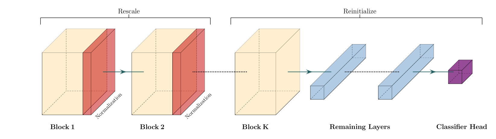
Figure 1: Given a deep neural network starting with $K$ convolutional blocks followed by other layers, lw proceeds sequentially from bottom to top (see Algorithm 1). When in block $k$ (e.g. $k=2$ in the figure above), the weights of all early blocks $\{1,\ldots,k\}$ are rescaled while subsequent layers are reinitialized. In addition, a normalization layer is inserted following block $K$.

Input: (1) Neural network with identified sequence of $K\geq 1$ conv blocks; (2) Training dataset; (3) $N\geq 1$.

Output: Trained model parameters.

Training:

1:Initialize the neural network architecture and record the scales of each layer during initialization;

2:for $k\in(1,2,\ldots,K)$ do

3:     for $n\in(1,2,\ldots,N)$ do

4:         Rescale the weights of all blocks $\{1,2,\ldots,k\}$;

5:         Compute $Z$: the output of Block $k$ of a sample $X$;

6:         Compute $\mu,\sigma\in\mathbb{R}$: mean and standard deviation of $Z$;

7:         if $n=1$ then

8:              Insert a lambda layer $\lambda x:(x-\mu)/\sigma$ after block $k$;

9:         else

10:              Update lambda layer with new values of $\mu$ and $\sigma$;

11:         end if

12:         Reinitialize all layers above block $k$;

13:         Fine-tune the entire model until convergence;

14:     end for

15:end for

Algorithm 1 Pseudocode of lw

It is worth noting that fc is a special case of lw, in which $K=1$ and $N>1$. Besides the prominent role of reinitialization, lw includes normalization and rescaling, which we show in an ablation study in Appendix F to be important. Next, we illustrate the basic principles of these reinitialization methods on a minimal example with synthetic data.

1.1 Synthetic Data Example

Table 1: Test accuracy [%] for the synthetic data experiment of Section 1.1 with different signal strengths $\alpha$ and different reinitialization methods. We observe that all initialization methods (with the exception of dsd) improve generalization in this example setting with lw performing best. In addition, reinitialization methods also tend to reduce the variance of the test accuracy.

$\alpha$	bl	welsr	dsd	wels	fc	lw
0.5	$20.3$	$24.6$	$22.9$	$23.1$	$23.6$	$25.2$
	($\pm 0.6$)	($\pm 1.0$)	($\pm 0.6$)	($\pm 1.4$)	($\pm 3.0$)	($\pm 0.8$)
$1.0$	$50.7$	$72.9$	$53.4$	$66.1$	$68.6$	$72.3$
	($\pm 5.4$)	($\pm 0.9$)	($\pm 0.7$)	($\pm 2.1$)	($\pm 2.1$)	($\pm 3.6$)
$2.0$	$94.6$	$98.2$	$90.3$	$96.8$	$99.0$	$99.8$
	($\pm 2.0$)	($\pm 0.4$)	($\pm 1.4$)	($\pm 0.1$)	($\pm 0.2$)	($\pm 0.2$)

Setup.

Let $\textbf{x}\in{\mathbb{R}}^{128}$ be the instance and y be its label, which is sampled uniformly at random from the set $\{0,1,...,7\}$. For the instances, on the other hand, each of the first 3 coordinates of x is chosen from $\{-1,1\}$ to encode the label y appropriately in binary form. For example, instances that belong to the class 0 would have their first three coordinates as $(-1,-1,-1)$, whereas instances in class 5 would have $(1,-1,1)$. Consequently, the first three coordinates of an instance correspond to its “signal.” The remaining 125 entries of x are randomly sampled i.i.d. from ${\mathcal{N}}(0,\,1)$.

Although we focus in this work on convolutional neural networks (CNN), we use a multilayer perceptron (MLP) in this synthetic data experiment for illustration purposes because the inputs are not images but generic feature vectors. The MLP contains two hidden layers of 32 neurons with ReLU activations (Nair and Hinton 2010) followed by a classifier head with softmax activations. It optimizes the cross–entropy loss. We train on 256 examples using gradient descent with a learning rate 0.05.

Methods.

Treating every layer as a block, we have $K=3$. If $200$ training steps are used per round of reinitialization and $N=3$, lw trains the model once for $200$ steps after which the 2^nd and 3^rd layers are reinitialized (in addition to rescaling and normalization). This is carried out $N=3$ times in the first layer before $k$ is incremented. The same process is repeated on each layer making a total of $200\times N\times K=1,800$ training steps overall. In wels, welsr, dsd, and fc, the model is trained for $200$ steps before reinitialization is applied, and this is repeated $K\times N$ times for the same total of $1,800$ steps. The baseline method corresponds to training the model once without reinitialization for a total of $1,800$ training steps.

Results.

When trained for 1,800 steps, the baseline (bl) achieves 100% training accuracy, but only around 51% test accuracy. The large gap between training and test accuracy for such a simple task is reminiscent of the classical phenomenon of overfitting. Note that the number of training examples is 256, which is generally small for 128 features of equal variance. On the other hand, reinitialization improves accuracy as shown in Table 1 even though these reinitialization methods do not have access to any additional data and use the same optimizer and hyper-parameters as baseline training. The training accuracy is 100% in all cases. We also observe that reinitialization tends to reduce the variance of the test accuracy (with respect to the random seed).

In the above experiment, both the signal part (first three coordinates) and the noise part (remaining coordinates) have the same scale (standard deviation 1). We can make the classification problem easier or harder by multiplying the signal part by a signal strength $\alpha>1$ or $\alpha<1$, respectively. We present the average test accuracy in Table 1 for a selection of values of $\alpha$ with $N=3$. Appendix A contains additional results when weight decay is added.

1.2 Contribution

In this work, we introduce a new layerwise reinitialization algorithm lw, which outperforms previous methods. We provide two explanations, supported by experiments, for why it improves generalization in convolutional neural networks. First, we show that lw improves the margin on the training examples without increasing the norm of the weights, hence leading to an improvement in known margin-based generalization bounds in neural networks. Second, we show that lw settles in flatter local minima of the loss surface.

Furthermore, we provide a comprehensive study comparing previous reinitialization methods: First, we evaluate different methods within the same context. For example, the comparison in (Taha, Shrivastava, and Davis 2021) uses only a single reinitialization round of the dense-sparse-dense approach (dsd), while dsd can be extended to multiple rounds. Also, (Zhao, Matsukawa, and Suzuki 2018) uses an ensemble of classifiers when reinitializing the fully-connected layers, which could (at least partially) explain the improvement in performance. By contrast, we follow a coherent training protocol for all methods. Second, we use our empirical evaluation to analyze the effect of the experiment’s design, such as augmentation, dropout, learning rate, and momentum. The goal is to determine if the effect of reinitialization could be achieved by tuning such settings. Third, we employ decision tree classifiers to identify when each reinitialization method is likely to outperform others. In summary, we:

1. Introduce a new reinitialization method that is motivated by common observations of generalization and memorization effects across the neural network’s layers. We show that it outperforms other methods with a statistically significant evidence at the 95% level.

2. Suggest two explanations, supported by experiments, for why lw is more successful at improving generalization in CNNs compared to other methods.

3. Present a comprehensive evaluation study of reinitialization methods covering more than 2,000 experiments for four convolutional architectures: (1) simplified CNN, (2) VGG16 (Simonyan and Zisserman 2015), (3) MobileNet (Howard et al. 2017) and (4) ResNet50 (He et al. 2016b). We conduct the evaluation over 12 benchmark image classification datasets (cf. Appendix B).

2 Related Work

Reinitialization.

As stated earlier, a number of works suggest that reinitializing a subset of the neural network parameters during training can improve generalization. This includes, the dense-sparse-dense (dsd) training workflow proposed by  (Han et al. 2017), in which reinitialization occurs only once during training. However, as the authors argue, the improvement in accuracy in dsd could be attributed to the effect of introducing sparsity, not reinitialization. Another example is “Knowledge Evolution”, including weight level splitting (wels) and its randomized version (welsr) (Taha, Shrivastava, and Davis 2021). It was noted that wels outperformed welsr, which agrees with our observations. Finally, some recent works propose to reinitialize the fully-connected layers only (Li et al. 2020; Zhao, Matsukawa, and Suzuki 2018). In particular, reinitializing the last layer several times and combining the models into an ensemble can improve performance (Zhao, Matsukawa, and Suzuki 2018). However, the improvement in accuracy could (at least partially) be attributed to the ensemble of predictors, not to reinitialization per se. For fair comparison, we extend dsd to multiple rounds of reinitialization and do not use an ensemble of predictors.

Generalization Bounds.

Several generalization bounds for neural networks have been proposed in the literature. Of those, a prototypical approach is to bound the generalization gap by a particular measure of the size of weights normalized by the margin on the training set. Examples of measures of the size of weights include the product of the $\ell_{1}$ norms (Bartlett 1998) and the product of the Frobenius norms of layers (Neyshabur, Tomioka, and Srebro 2015), among others (Bartlett, Foster, and Telgarsky 2017; Neyshabur et al. 2017; Arora et al. 2018). While such generalization bounds are often loose, they were found to be useful for ranking models (Neyshabur et al. 2017). The fact that rich hypothesis spaces could still generalize if they yield a large margin over the training set was used previously to explain the performance of boosting (Schapire et al. 1997). In Section 4, we show that lw boosts the margin on the training examples without increasing the size of the weights.

Flatness of the Local Minimum.

Another important line of work examines the connection between generalization and the curvature of the loss at the local minimum (Keskar et al. 2016; Neyshabur et al. 2017; Foret et al. 2021). Deep neural networks are known to converge to local minima with sparse eigenvalues ($>$94% zeros) in their Hessian (Chaudhari et al. 2019). Informally, a flat local minimum is robust to data perturbation, and this robustness can, in turn, be connected to regularization (Bishop 1995). In fact, some of the benefits of transfer learning were attributed to the flatness of the local minima (Neyshabur, Sedghi, and Zhang 2020). For a precise treatment, one may use the PAC-Bayes framework to derive a generalization bound that comprises of two terms: (1) sharpness of the local minimum, and (2) the weight norm over noise ratio (Neyshabur et al. 2017). Similar terms also surface in the notion of “local entropy” (Chaudhari et al. 2019). We show in Section 4 that lw improves both terms.

Generalization vs. Memorization.

Several works point out that early layers in a neural network tend to learn general-purpose representations whereas later layers specialize, e.g. (Raghu et al. 2019; Arpit et al. 2017; Yosinski et al. 2014; Maennel et al. 2020). This can be observed, for instance, using probes, in which classifiers are trained on the layer embeddings. As demonstrated in (Cohen, Sapiro, and Giryes 2018) and (Baldock, Maennel, and Neyshabur 2021), deep neural networks learn to separate classes at the early layers with real labels (generalization) but they only separate classes at later layers when the labels are random (memorization). One explanation for why lw improves generalization is that it encourages learning general rules at early layers and discourages memorization at later layers.

Table 2: Test accuracy results [%] for the five reinitialization methods across 12 benchmark datasets. Reinitialization improve generalization, in general, with lw often outperforming others. These numbers include data augmentation; see Appendix C for more results with different experiment settings. The abbreviations b,r,d,w,f,l stand for baseline, welsr, dsd, wels, fc, and lw, respectively. In lw , $N=1$. Also, every reinitialization method uses the same number of rounds $K$, where $K$ depends on the model architecture (cf. Appendix B). Note that we do not fine-tune the hyper-parameters $N$ and $K$. In the baseline method, which trains only once, we increase the maximum number of training steps to match that of reinitialization methods. In wels, welsr, and dsd, we follow (Taha, Shrivastava, and Davis 2021) in having 20% of the parameters reinitialized.

Dataset	Model	b	r	d	w	f	l
oxford-iiit	scnn	15.1	14.6	14.3	14.7	16.0	16.6
	vgg16	22.0	20.0	20.9	20.7	39.1	29.8
	mobilenet	27.7	24.1	23.2	24.3	23.5	41.7
	resnet50	29.7	33.3	39.1	31.9	36.6	34.4
dogs	scnn	07.4	08.2	07.7	08.0	08.1	08.6
	vgg16	16.0	16.9	15.5	16.7	37.3	31.2
	mobilenet	19.0	19.5	27.1	18.8	20.7	35.8
	resnet50	26.4	30.7	28.4	35.2	33.3	36.9
fmnist	scnn	92.3	92.3	92.2	92.2	92.5	92.7
	vgg16	90.7	92.3	91.5	92.3	92.1	92.8
	mobilenet	91.7	92.0	92.4	92.0	91.5	92.7
	resnet50	92.9	92.7	93.0	92.9	93.2	93.4
cars196	scnn	05.6	06.0	05.3	05.5	07.3	05.8
	vgg16	11.7	10.7	11.2	11.4	43.6	22.4
	mobilenet	06.9	16.2	09.1	11.9	13.8	44.0
	resnet50	21.8	42.5	33.2	43.1	36.7	43.6
mnist-cor	scnn	99.0	99.0	99.0	99.0	99.0	99.0
	vgg16	99.0	98.9	98.9	98.9	99.0	99.0
	mobilenet	98.9	98.8	98.9	98.8	98.9	99.0
	resnet50	99.1	99.0	99.1	99.1	99.0	99.1
cifar10-cor	scnn	82.4	83.8	82.7	83.3	84.2	84.8
	vgg16	83.6	86.5	84.7	85.8	84.7	88.3
	mobilenet	85.8	86.6	87.4	87.4	86.0	87.4
	resnet50	88.0	87.4	89.2	89.1	88.7	88.3
cifar10	scnn	82.7	84.2	82.5	83.7	84.9	84.3
	vgg16	84.7	86.8	84.9	85.9	85.0	88.9
	mobilenet	86.4	86.6	88.1	86.5	86.3	87.6
	resnet50	87.4	87.5	88.9	89.6	89.2	89.1
caltech101	scnn	50.1	52.2	52.2	51.5	54.4	52.8
	vgg16	55.9	55.8	57.1	56.3	67.1	59.1
	mobilenet	41.0	41.5	47.4	41.8	48.0	46.3
	resnet50	50.2	51.9	53.1	57.5	52.1	50.5
cassava	scnn	58.9	60.6	59.4	62.2	67.0	69.3
	vgg16	70.3	70.0	70.0	71.2	71.5	68.3
	mobilenet	62.3	72.8	80.1	76.1	77.3	81.1
	resnet50	46.5	79.2	82.9	82.6	77.6	73.9
cmaterdb	scnn	96.2	97.0	96.6	97.3	97.4	97.1
	vgg16	97.5	98.2	97.1	97.5	97.5	97.5
	mobilenet	97.9	97.4	97.7	98.0	97.5	97.0
	resnet50	97.4	97.9	97.7	97.4	97.7	98.4
birds2010	scnn	03.8	03.7	04.0	03.2	04.2	03.8
	vgg16	05.5	06.5	05.6	05.8	13.2	09.8
	mobilenet	06.6	09.0	08.1	06.2	07.4	09.8
	resnet50	08.5	12.5	11.2	13.0	11.9	10.6
cifar100	scnn	53.9	55.0	53.2	53.8	58.0	58.0
	vgg16	53.2	60.2	53.1	57.6	55.2	64.3
	mobilenet	57.3	59.3	60.6	65.2	57.1	57.8
	resnet50	59.9	60.0	61.8	62.1	60.3	60.7

3 Empirical Study

We begin by evaluating the performance of the five reinitialization methods discussed in Section 1 for four convolutional architectures on 12 benchmark datasets including, for example, CIFAR10/100 (Krizhevsky 2009), Fashion MNIST (Xiao, Rasul, and Vollgraf 2017), and Caltech101 (Fei-Fei, Fergus, and Perona 2004), among others (see Appendix B for details). All images are resized to $224\times 224$. The architectures are (1) simplified CNN, (2) VGG16 (Simonyan and Zisserman 2015), (3) MobileNet (Howard et al. 2017) and (4) ResNet50 (He et al. 2016b). We denote these by scnn, vgg16, mobilenet, and resnet50, respectively. We use He-initialization (He et al. 2015) for all models unless stated otherwise.

To recall, every reinitialization method trains the same model on the same dataset for several rounds. After each round, a binary mask of the model parameters is selected according to the reinitialization criteria and the update in Eq. (1) is applied for some random initialization $\eta$. After that, the model is fine-tuned on the same data. Blocks lwcorrespond to the standard blocks of the architecture (e.g. a block in Figure 1 would correspond to either an identity or a convolutional block in ResNet50). Also, 10% of the training split is reserved as validation set, which is used for early stopping in all methods.

To evaluate the relative performance of the reinitialization methods we perform a set of experiments in which we fix the hyperparameters for all architectures and datasets to the same values. The hyperparameters were chosen to work reasonably well across all combinations; in particular they enable reaching 100% training accuracy in all cases. We use SGD with an initial learning rate of 0.003 and momentum 0.9. The learning rate is decreased by a factor of 2 whenever the validation error does not improve for 20 epochs. The batch size is 256 and a maximum of 100k minibatch steps are used. We run all experiments, as explicitly stated, without data augmentation or with mild augmentation consisting of horizontal flipping and random cropping (in which the size is increased to $248\times 248$ before a crop of size $224\times 224$ is selected). Such fixed hyperparameters are suboptimal for some combinations of architectures and datasets and therefore the resulting numbers can be worse than state-of-the-art results. However, they enable reaching 100% training accuracy in all combinations of models and datasets. For example, increasing the learning rate to 0.01 would prevent ResNet50 from progressing its training error beyond that of random guessing on the cassava dataset.

Table 3: Significance analysis: A star ($\star$) in a cell indicates that the method in column outperforms the method in row with statistically significant evidence at the $95\%$ confidence level, computed using the exact binomial test. A circle ($\circ$) indicates that the significance test continues to hold even after applying Holm’s step-down correction for multiple hypothesis tests (Demšar 2006). There is no architecture where an algorithm outperforms lw statistically significantly, so the last (empty) row is omitted.

	scnn						vgg16						mobilenet						resnet50
	b	r	d	w	f	l	b	r	d	w	f	l	b	r	d	w	f	l	b	r	d	w	f	l
b					$\circ$	$\circ$		$\circ$		$\circ$	$\circ$	$\circ$			$\circ$	$\star$		$\circ$		$\circ$	$\circ$	$\circ$	$\circ$	$\circ$
r					$\circ$	$\circ$						$\circ$						$\circ$				$\circ$		$\star$
d		$\star$			$\circ$	$\circ$		$\circ$		$\star$	$\circ$	$\circ$						$\circ$
w					$\circ$	$\circ$					$\star$	$\circ$						$\circ$
f																		$\circ$				$\circ$

Table 2 provides the detailed results of the five reinitialization methods across the benchmark datasets with augmentation. Appendix C includes detailed results when other experiment settings are used. We now re-run these experiments with varying settings including augmentation (with/without), dropout rate (0 or 0.25) (Srivastava et al. 2014), and initializer (He normal (He et al. 2015) or Xavier uniform (Glorot and Bengio 2010)) and then aggregate the observations regarding which reinitialization method performs better than others (and the baseline). We perform an exact binomial test to evaluate which method performs statistically significantly better across the settings. In Table 3, we summarize these results. We observe that all reinitialization methods perform better than the baseline. In addition, lw outperforms the other methods with a statistical significant evidence at the 95% confidence level. Moreover, fc performs generally better than wels, welsr, and dsd. It is worth reiterating, that fc is a special case of lw that corresponds to $K=1$ and $N>1$.

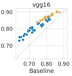
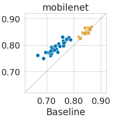
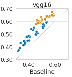
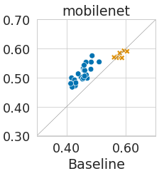
Figure 2: The test accuracy is displayed for the baseline ($x$-axis) vs. lw ($y$-axis) with $N=1$ for both vgg16 and mobilenet on CIFAR10 (top) and CIFAR100 (bottom). Amber dots are for experiments with augmentation while blue dots correspond to experiments without augmentation.

In Figure 2 we highlight a different view of the space of hyperparameters and reinitialization: For the architectures vgg16 and mobilenet and the popular datasets CIFAR-10/100, we plot the results for a wider range of hyperparameters and compare the resulting accuracies for the baseline and lw. Example of hyperparameters that we vary include the learning rate ($0.001$, $0.003$, or $0.01$), dropout rate ($0$, $0.25$, or $0.5$), momentum ($0$ or $0.9$), weight decay ($0$ or $10^{-5}$), and initializer (He normal or Xavier uniform). We observe that lw consistently outperforms the baseline. Further, the resulting accuracies range up to results that are as expected in the ‘vanilla’ setting we are considering here (without heavily tuning e.g. augmentation and regularization). Of course, better results can still be achieved when aiming for state-of-the-art results, see e.g. (Foret et al. 2021) for an in-depth discussion of the current best results on the CIFAR-10/100.

3.1 Effect of Experiment Design

To determine when a particular reinitialization method outperforms others, we train a decision tree classifier on the outcomes of several experiments that vary in design by, for example, the choice of the initializer (He normal or Xavier uniform), augmentation, and dropout. Every setting contains experiment runs of each of the 5 reinitialization methods in addition to the baseline for the four architectures and 12 benchmark datasets.

Figure 3: A decision tree classifier trained to predict the best reinitialization method based on the experiment design. The features are the training set size, number of classes, neural network architecture, dropout rate, augmentation, and the choice of initializer. When node impurity is large, i.e. Gini index $>0.5$, we report the top performing methods in the corresponding leaf.

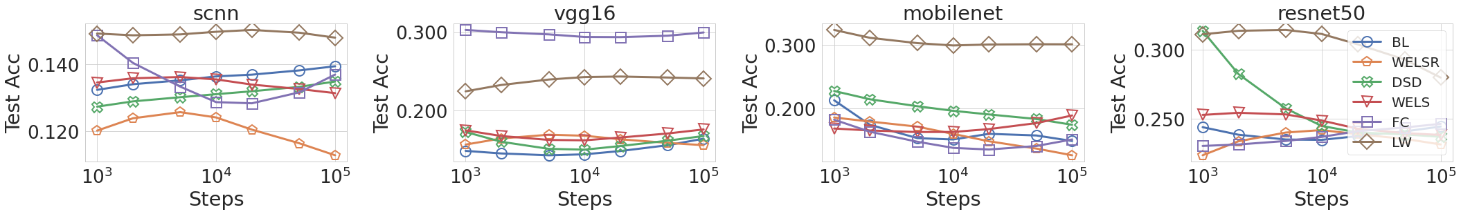
Figure 4: The test accuracy of reinitialization methods with different compute budgets plotted for Oxford-IIIT dataset (see Appendix G for full results on all datasets). The $x$-axis is the number of training steps per reinitialization round. For the baseline, the test accuracy is plotted over the same total number of steps as reinitialization. Most reinitialization methods quickly surpass the accuracy of the baseline for the same amount of compute.

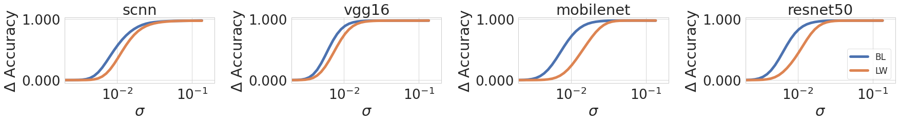
Figure 5: Bi-criteria plots for the change in training accuracy ($y$-axis) when the model parameters are perturbed by standard Gaussian noise $\mathcal{N}(0,\sigma^{2}I)$ for the Oxford-IIIT dataset. Lower curves suggest flatter local minima and better generalization. See Appendix G for full results on all datasets.

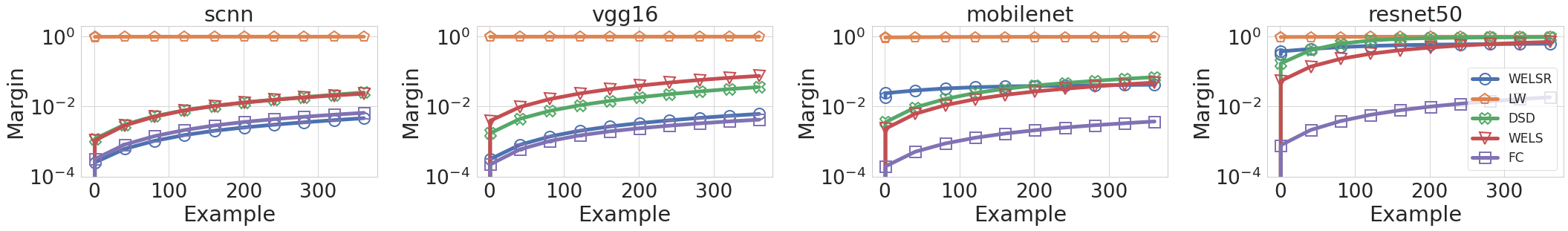
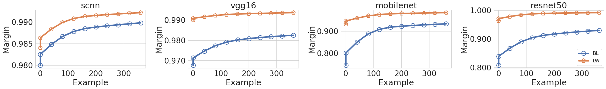
Figure 6: top: The smallest 400 margins in the training sample are plotted for different reinitialization methods in the Oxford-IIIT dataset. lw (orange) boosts the margin considerably compared to previous reinitialization methods. bottom: A comparison of the 400 smallest margins in the training sample between lw and bl. The curves are displayed separately for a better visualization, as they almost coincide in the wide ranged log-scale in the top two rows. Appendix G contains full results on all datasets.

3.2 Sharpness of the Local Minima

We use the decision tree classifier, implemented using the Scikit-Learn package (Pedregosa et al. 2011), for interpretability. The goal is to predict which reinitialization method performs best. Two features related to the dataset are included: the training set size and the number of classes. We use a minimum leaf size of 7 in the decision tree and a maximum depth of 4. Figure 3 displays the resulting decision tree. First, we observe that lw improves performance across the majority of combinations. The only exception is using ResNet50 with large training sets, in which most methods perform as well as the baseline.

3.3 Compute

In Table 2, every reinitialization round is trained until convergence. However, improvements in generalization can also be obtained at lower computational overhead by stopping earlier than at convergence in each round. This is illustrated in Figure 4. As shown in the figure, stopping early per round allows to realize the gain of reinitialization without incurring significant additional overhead. In addition, we show in Appendix E that training is faster in subsequent rounds of reinitialization.

4 Analysis

4.1 Boosting the Margin

As discussed earlier in Section 2, a typical approach for bounding the generalization gap in deep neural networks is to use a particular measure of the size of the weights normalized by the margin on the training sample. Let $D$ be the number of layers in a neural network, whose output is a composition of functions: $f(x)=f_{1}\circ f_{2}\circ\cdots f_{D}(x)$, where each $f_{i}(x)$ is of the form $f_{i}(x)=\sigma(W_{i}x)$ for some matrix $W_{i}$ and ReLU activation $\sigma$. Then, one measure of the size of the weight that relates to generalization is the product of the Frobenius norms of layers $\prod_{i=1}^{d}||W||_{F}^{2}$ (Neyshabur, Tomioka, and Srebro 2015; Neyshabur et al. 2017). This is normalized by the margin $\gamma>0$ on the training examples, which is the smallest difference between the score assigned to the true label and the next largest score. For a better visualization, we use the margin of the softmax output since it is normalized in the interval $[0,\,1]$.

Figure 6 displays the smallest 400 margins on the training sample for Oxford-IIIT dataset. Appendix G contains full results on all datasets. As shown in the figure, lw boosts the margin on the training sample considerably when compared to previous reinitialization methods. Most importantly, lw achieves this without increasing the size of the weights. To take the contribution of the normalization layers into account when calculating the product $\prod_{i=1}^{d}||W||_{F}^{2}$, we compare the product of the norms of the input to the classifier head (activations) and the norm of the weights of the classifier head in each method. We observe that lw tends to maintain the same size of the weights as the baseline. Appendix D provides further details.

We provide an informal argument for why this happens. First, the product of the norms of the weights in the identified $K$ blocks in lw (cf. Figure 1 and Algorithm 1) tend to remain unchanged due to the normalization layers inserted after each round. What changes is the norm of the final layers (following block $K$), but their norm tends to shrink because they train from scratch faster with each round (cf. Appendix E). As for the margin, because the network classifies all examples correctly in a few epochs in the final round of lw, any additional epochs have the effect of increasing the margin to reduce the cross entropy loss.

4.2 Sharpness of the Local Minima

Finally, we observe that the final solution provided by lw seems to reside in a “flatter” local minima of the loss surface than in the baseline. One method for quantifying flatness is to compare the impact on the training loss when the model parameters are perturbed by some standard Gaussian noise, which can be linked to generalization via explicit bounds (Neyshabur et al. 2017). To recall, both lw and bl share the same size of the weights (cf. Appendix D). Figure 5 shows that the solution reached by lw is more robust to model perturbation than in standard training. More precisely, for every amount of noise added into the model parameters w, the change in the training loss in lw is smaller than in standard training suggesting that the local minimum is flatter in lw.

5 Discussion

In this paper, we present a comprehensive evaluation of reinitialization algorithms and introduce a new method that outperforms others. Empirical results show that this method improves generalization across a wide range of architectures and hyper-parameters, particularly for small datasets. It relates to prior works that distinguish learning general rules in earlier layers from exceptions to the rules in later layers, because lw places more emphasis on the early layers of the neural network. We also argue that the improved generalization can be connected to the sharpness of the local minima and the margins on the training examples, and conducted further ablation and failure analyses using decision trees.

Our takeaway message is that the accuracy of convolutional neural networks can be improved for small datasets using bottom-up layerwise reinitialization, where the number of reinitialized layers may vary depending on the available compute budget. At one extreme, one would benefit from reinitializing the classifier’s head alone, but reinitializing all layers in sequence with rescaling and normalization yields better results. For large datasets, however, reinitialization does not seem to offer a benefit. We hope that the description of the observed positive effects will inspire others to study them more and to develop more efficient alternatives.

Appendix A Synthetic Data Experiment

We use the same type of data as described in Section 1.1, but look in more detail at the more difficult case $\alpha=0.5$, this means the first three entries of the data encode the 8 possible labels as the 8 corners of the cube $[-0.5,0.5]^{3}$, whereas the remaining entries are still sampled from the standard normal distribution. In addition, one may add a weight decay penalty to the task and examine the impact of rescaling alone. Specifically, we consider two cases:

• Rescaling: Instead of training once for $N$ epochs, we train 5 times for $N/5$ epochs, and in between we scale back all weights such that the norm of each layer matches the norm after initialization.

• Reinitialization: In addition to rescaling, we re-initialize the layers above the first one in the first two rounds, above the second layer in the next two rounds, and only the top layer in the last round.

The results are shown in Table 4. We use the same type of data as described above, but focus now at the more difficult case of $\alpha=0.5$.

We observe that one can get significantly better results with weight decay. Nevertheless, lw gives an additional benefit on top of the L2 regularization. In this particular experiment, rescaling seems to have the biggest effect but this is not generally the case in natural image datasets, in which the gain seems to be modest without reinitialization.

Table 4: Test accuracies (average of 100 runs)

L2 penalty	Baseline	Rescaling	lw
0.000	0.19	0.21	0.25
0.005	0.51	0.67	0.82
0.010	0.54	0.89	0.85
0.020	0.58	0.87	0.86
0.050	0.77	0.78	0.79
0.100	0.59	0.63	0.64

Appendix B Experiment Setup

B.1 Architectures

Throughout the main text, we use four different architectures: one simple convolutional neural network, and three standard deep convolutional models.

In all architectures, we use weight decay with penalty $10^{-5}$ unless explicitly stated otherwise. We also use layer normalization (Ba, Kiros, and Hinton 2016), implemented in TensorFlow (Abadi et al. 2015) using GroupNormalization layers with groups=1. Similar results are obtained when using Batch Normalization (Ioffe and Szegedy 2015).

In all experiments, we use SGD as an optimizer. Unless explicitly stated otherwise, we use a learning rate of 0.003 and momentum 0.9. Also, we use a batch size of 256. All experiments are executed on Tensor Processing Units for a maximum of 100,000 minibatch steps per reinitialization round. We resize images to $224\times 224$ in all experiments.

Simple CNN (scnn).

This architecture contains four convolutional blocks followed by one dense layer before the classifier head. The number of convolutional blocks $K$ used in this architecture is 4. Every convolutional block is a 2D convolutional layer, followed by layer normalization and ReLU activation. Precisely:

    conv2d              32 filters
    layer_norm;
    activation_relu

    conv2d              32 filters
    layer_norm;
    activation_relu
    max_pooling2d

    conv2d              64 filters
    layer_norm;
    activation_relu

    conv2d              64 filters
    layer_norm;
    activation_relu
    max_pooling2d

    flatten
    dense              512 units
    layer_norm;
    activation_relu
    dropout

    classifier_head

MobileNetV1 (mobilenet).

This is the standard shallow MobileNet architecture (Howard et al. 2017). The standard blocks in this architecture are either convolutional blocks with layer normalization and ReLU or depthwise separable convolutions with depthwise and pointwise layers followed by layer normalization and ReLU (see Figure 3 in Howard et al. (2017)). In the shallow architecture, the number of convolutional blocks $K$ is 7.

VGG16 (vgg16).

This is the standard VGG16 architecture (Simonyan and Zisserman 2015). The standard blocks in this architecture are convolutional layers with layer normalization and ReLU (see Table 1 in Simonyan and Zisserman (2015)). The number of convolutional blocks $K$ is 13.

ResNet50 (resnet50).

This is the standard ResNet50 architecture (He et al. 2016a). The standard blocks in this architecture either identity blocks or convolutional blocks (see Table 1 in He et al. (2016a)). The number of convolutional blocks $K$ used in this architecture is 16.

B.2 Datasets

The 12 benchmark datasets are all taken from the Tensorflow dataset repository (Abadi et al. 2015). Table 5 gives an overview of each dataset.

Table 5: Overview of the 12 benchmark datasets.

Name	—Training—	—Test—	# Classes
oxford-iiit	03,680	03,669	037
(Parkhi et al. 2012)
dogs	12,000	08,580	120
(Khosla et al. 2011)
fmnist	60,000	10,000	010
(Xiao, Rasul, and Vollgraf 2017)
cars196	08,144	08,041	196
(Krause et al. 2013)
mnist-cor	60,000	10,000	010
(Mu and Gilmer 2019)
cifar10-cor	50,000	10,000	010
(Hendrycks and Dietterich 2019)
cifar10	50,000	10,000	010
(Krizhevsky 2009)
caltech101	03,060	06,084	101
(Fei-Fei, Fergus, and Perona 2004)
cassava	05,656	01,885	004
(Mwebaze et al. 2019)
cmaterdb	05,000	01,000	010
(Das et al. 2012)
birds2010	03,000	03,033	200
(Welinder et al. 2010)
cifar100	50,000	10,000	100
(Krizhevsky 2009)

Appendix C Detailed Empirical Evaluation Results

As stated earlier in Section 3, Table 2 provides the results when augmentation is used but without dropout. We provide here two other settings: without augmentation and dropout and with both augmentation and dropout. We use the same other hyperparameters described in Section 3. Table 6 provides the results without augmentation and without dropout. Table 7 provides the results with both augmentation and dropout. We did not run the combination of dropout without augmentation.

Table 6: Test accuracy results [%] for the five reinitialization methods across 12 benchmark datasets. All reinitialization methods improve generalization, with lw outperforming others in most cases. Here no data augmentation or dropout are used, see Table 2 for results with data augmentation and Table 7 for results with both augmentation and dropout.

Dataset	Model	b	r	d	w	f	l
oxford-iiit	scnn	13.7	12.0	13.4	14.0	14.0	15.0
	vgg16	16.2	16.7	16.9	16.4	29.7	25.6
	mobilenet	13.4	13.8	17.2	15.9	14.8	30.1
	resnet50	24.0	24.2	22.9	24.9	23.7	28.5
dogs	scnn	05.8	05.2	05.2	05.1	05.1	06.1
	vgg16	11.4	11.8	10.7	10.3	24.2	19.1
	mobilenet	09.7	08.6	09.0	11.6	09.9	19.2
	resnet50	14.0	17.5	19.2	16.0	13.9	22.0
fmnist	scnn	91.8	91.7	91.7	91.7	91.8	92.1
	vgg16	92.4	92.6	92.4	92.6	92.7	92.5
	mobilenet	92.2	91.7	91.8	91.9	91.9	92.6
	resnet50	89.9	89.7	89.9	90.0	90.1	90.2
cars196	scnn	03.4	03.4	03.4	03.5	03.2	03.8
	vgg16	06.5	05.5	07.7	07.0	20.9	09.9
	mobilenet	06.1	08.9	05.3	07.4	06.8	22.2
	resnet50	10.1	12.8	13.4	13.7	10.4	12.6
mnist-cor	scnn	99.2	99.3	99.3	99.3	99.4	99.4
	vgg16	99.3	99.3	99.4	99.4	99.4	99.5
	mobilenet	99.5	99.4	99.4	99.3	99.4	99.5
	resnet50	99.0	99.1	99.0	99.1	99.2	99.0
cifar10-cor	scnn	71.8	75.1	73.7	75.7	74.9	75.2
	vgg16	76.7	79.2	78.5	80.5	77.7	81.6
	mobilenet	78.3	78.4	78.0	78.4	79.2	83.6
	resnet50	68.4	69.2	71.3	70.8	69.4	69.7
cifar10	scnn	72.2	75.1	74.5	75.9	74.8	75.9
	vgg16	76.8	79.3	78.6	80.8	77.4	81.4
	mobilenet	77.7	77.7	78.7	79.8	79.3	83.6
	resnet50	68.8	70.4	71.2	71.0	69.2	70.2
caltech101	scnn	51.1	49.9	49.8	48.4	50.8	50.7
	vgg16	54.1	55.4	54.2	55.9	69.1	57.3
	mobilenet	36.7	43.0	44.9	40.9	42.3	47.0
	resnet50	50.4	54.6	55.0	52.9	50.7	53.3
cassava	scnn	59.4	58.6	58.6	59.8	61.6	63.9
	vgg16	58.4	59.5	58.4	62.1	58.5	59.3
	mobilenet	52.6	57.9	63.6	62.2	55.4	70.0
	resnet50	61.9	57.3	62.8	58.1	56.7	63.9
cmaterdb	scnn	97.1	97.0	96.9	97.3	97.4	97.4
	vgg16	97.8	97.2	97.5	97.5	97.7	99.0
	mobilenet	98.6	98.6	98.6	98.6	98.1	98.6
	resnet50	94.5	94.9	97.1	95.9	96.7	95.8
birds2010	scnn	02.0	02.6	02.3	02.2	02.4	02.4
	vgg16	03.8	04.3	04.1	03.4	08.5	05.1
	mobilenet	04.5	03.9	05.2	05.9	05.3	08.1
	resnet50	06.9	08.7	10.0	10.0	06.5	10.0
cifar100	scnn	39.8	42.2	39.5	40.5	43.7	43.8
	vgg16	45.2	48.4	47.9	51.6	45.2	51.2
	mobilenet	44.7	46.1	54.3	44.3	42.0	50.9
	resnet50	36.4	37.5	40.4	38.9	36.7	38.0

Table 7: Test accuracy results [%] for the five reinitialization methods across 12 benchmark datasets. All reinitialization methods improve generalization, with lw outperforming others in most cases. Here both data augmentation and dropout are used, see Table 2 for results with data augmentation but no dropout and Table 6 for results without augmentation or dropout.

Dataset	Model	b	r	d	w	f	l
oxford-iiit	scnn	15.8	13.6	14.3	15.1	19.3	17.1
	vgg16	25.3	26.7	26.6	26.4	43.4	34.4
	mobilenet	28.4	29.1	27.8	27.9	22.0	41.0
	resnet50	33.1	35.2	41.2	37.4	32.6	35.6
dogs	scnn	08.4	08.9	07.6	08.0	09.6	09.1
	vgg16	17.7	19.7	19.5	18.9	34.9	35.9
	mobilenet	17.8	23.5	27.3	22.4	20.5	35.0
	resnet50	30.7	33.3	33.1	33.8	34.5	40.1
fmnist	scnn	93.1	93.0	92.8	93.2	93.3	93.0
	vgg16	91.7	92.4	91.7	92.1	92.4	93.0
	mobilenet	91.6	91.7	91.7	92.1	91.7	92.9
	resnet50	93.1	93.3	93.2	93.4	92.9	93.4
cars196	scnn	06.3	06.2	05.9	06.8	07.4	06.4
	vgg16	14.3	18.9	12.6	16.6	45.2	34.2
	mobilenet	09.5	16.1	30.8	24.1	16.4	44.5
	resnet50	19.8	45.7	43.0	48.1	45.0	47.5
mnist-cor	scnn	99.0	99.0	99.1	98.9	99.2	99.0
	vgg16	98.9	99.0	99.0	99.0	99.0	99.2
	mobilenet	98.8	99.0	99.0	98.9	99.0	99.0
	resnet50	99.1	99.1	99.1	99.1	99.1	99.1
cifar10-cor	scnn	84.0	85.3	84.9	85.0	85.2	85.8
	vgg16	84.8	86.5	84.9	85.9	85.4	88.8
	mobilenet	85.9	87.2	88.2	88.3	85.8	87.0
	resnet50	89.5	89.6	90.7	90.0	90.3	89.1
cifar10	scnn	84.6	86.0	85.8	85.4	85.9	85.6
	vgg16	85.0	87.1	85.3	85.6	85.9	89.5
	mobilenet	86.6	86.9	88.3	88.5	86.7	87.4
	resnet50	89.6	90.0	90.7	91.2	89.7	89.5
caltech101	scnn	51.4	53.5	51.1	52.6	52.4	53.6
	vgg16	59.6	61.7	60.8	61.0	68.1	62.7
	mobilenet	47.1	43.0	47.5	45.6	51.3	49.4
	resnet50	50.6	54.1	54.6	55.7	51.4	50.3
cassava	scnn	61.8	62.9	60.7	61.9	68.4	68.8
	vgg16	70.1	71.4	73.7	71.0	71.1	71.9
	mobilenet	68.5	70.0	78.6	74.3	73.7	80.5
	resnet50	74.2	77.6	81.5	80.9	73.5	78.6
cmaterdb	scnn	97.0	97.4	98.7	97.7	97.9	97.7
	vgg16	97.9	97.7	97.9	97.8	98.3	97.8
	mobilenet	97.4	98.6	97.9	97.5	97.3	98.2
	resnet50	97.8	97.5	98.0	97.8	98.6	98.6
birds2010	scnn	04.0	04.0	03.5	03.7	03.3	04.4
	vgg16	06.5	08.1	08.5	08.1	18.6	12.6
	mobilenet	02.5	09.6	05.1	06.3	08.4	09.0
	resnet50	11.5	14.8	13.3	15.2	13.5	13.3
cifar100	scnn	57.0	56.9	56.9	58.3	58.8	58.8
	vgg16	56.7	61.1	57.2	58.5	57.4	64.5
	mobilenet	58.0	60.6	60.4	64.8	58.2	58.1
	resnet50	59.6	61.4	61.8	63.5	63.1	62.2

Appendix D Size of the Weights

To calculate the norm of the weights while taking the contribution of the normalization layers into account, we compute the norm of the input to the classifier head (activations) for a random training sample of size 256. Then, we compute the Frobenius norm of the weights at the classifier head. Finally, we compute their product, which reflects the product of the Frobenius norm of layers stated in the generalization bound. Figure 7 shows a a Gaussian approximation to the ratio of the size of the weights of each reinitialization method over the size of the weights in the baseline. As shown in the figure, lw tends to maintain the size of the weights, while also boosting the margin on the training examples as discussed in Section 4

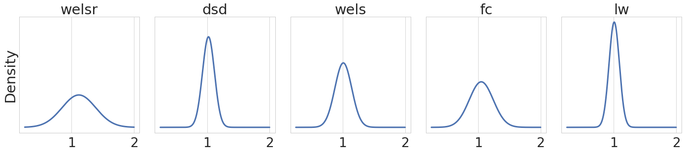
Figure 7: For each reinitialization method, the Gaussian approximation of the density of the ratio of the size of the weights over the size of the weights in the baseline method is shown. The density of the ratio in lw is concentrated around 1, which implies that lw tends to not increase the size of the weights.

Appendix E Training Speed

It is worth highlighting that while lw involves multiple rounds of training the whole model, training is often much faster in subsequent rounds. This is illustrated in Figure 8 for the vgg16 architecture. The experiment settings used to create Figure 8 are:

Learning Rate	0.003
Momentum	0
Weight Decay	1e-5
Augmentation	No
Dropout	0
Initializer	He Normal

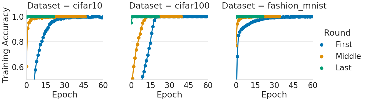
Figure 8: Training accuracy plotted against epochs in the first, middle, and last rounds of lw with $N=1$ in vgg16 (see Appendix E). A training round corresponds to fine-tuning the model until convergence. While lw involves multiple rounds of training, training can be much faster in subsequent rounds.

Appendix F Ablation

lw includes rescaling, normalization, and reinitialization. In some cases, these may not all be required and reinitialization alone suffices, but this is not always the case. We observe a consistent improvement in lw when rescaling and normalization are included, in addition to fine-tuning the whole model at each round. In general:

• The improvement in generalization in lw cannot be attributed to rescaling or normalization alone. Reinitialization has the main effect.

• There exist experiment designs in which reinitialization fails without normalization or fine-tuning the model.

• We observe cases in which rescaling alone helps but adding reinitialization improves performance further.

• The gain from lw cannot be obtained by just training the baseline longer (i.e. using the same computational budget).

In this section, we show that the primary effect in lw comes from reinitialization, and that the improvement in generalization cannot be attributed to rescaling or normalization alone. We also show that fine-tuning the whole model performs better than freezing the early layers. Finally, we illustrate a case where lw without normalization fails.

Rescaling.

In the synthetic data experiment in Appendix A, we show that rescaling improves performance compared to the baseline but adding re-initializations improves it further.

Reinitialization.

We use the vgg16 architecture with the same hyperparameters as listed in Appendix E.

We train it on CIFAR10 and CIFAR100. First, we observe that applying the same sequential process with rescaling and normalization but without reinitialization does not have an impact on the test accuracy. The test accuracy in CIFAR10 remains at around 66% and in CIFAR100 at around 34% in all rounds, similar to the baseline (this is different from the results in Table 6 because momentum is not used here). When reinitialization is added, we obtain the familiar looking curves where the test accuracy improves steadily with each round. In particular, it reaches around 75% in CIFAR10 and around 42% in CIFAR100. This shows that the improvement in lw cannot be attributed to normalization or rescaling alone.

Fine-tuning vs. Freezing.

lw fine-tunes the entire model in each round. One alternative approach is to freeze the early blocks. However, because of the co-adaptability between neurons that arises during training (Yosinski et al. 2014), freezing some layers and fine-tuning the rest is difficult to optimize and can harm its performance (Yosinski et al. 2014). This is also true for reinitialization methods in general. Hence, the entire model including the kept layers is fine-tuned at each round.

We illustrate this with one example. The architecture is vgg16 on CIFAR100 but without normalization layers. If we apply lw while freezing the early layers instead of fine-tuning them, the training accuracy stays at 100% after each round until about round 5 before it drops to 1% and stays at 1% training accuracy throughout the subsequent rounds. Fine-tuning the whole model does not exhibit this behavior.

Normalization.

lw inserts normalization layers after each round with no trainable parameters. To illustrate why normalization is important, let the architecture be vgg16 on CIFAR100 again but without normalization layers. If we apply lw without adding normalization, the test accuracy drops from about 34% to 24%. With the normalization layers inserted by lw, it improves to 42%.

Training Longer.

The improvement in lw cannot be obtained by simply training longer even with learning rate scheduling. Throughout our experiments (e.g. Tables 2 and 6), we also train the baseline longer to have the same number of training steps in total as reinitialization methods. Despite that, reinitialization methods improve performance considerably.

Appendix G Complete Figures for all Datasets

For completeness, we provide the full version of Figures 4, 6, and 5 in this section. These are provided in Figures 9, 10, 11, and 12.

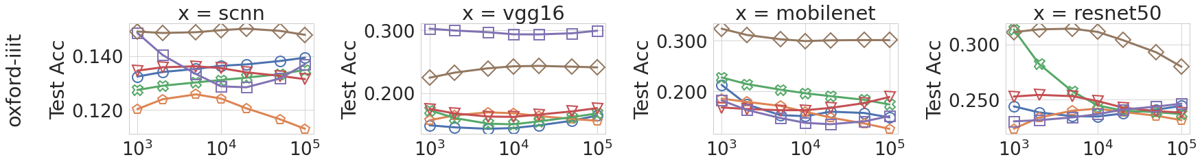
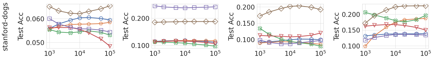
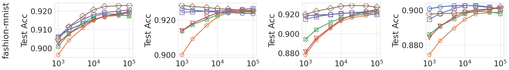
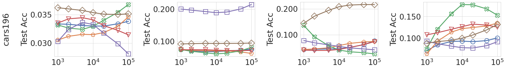
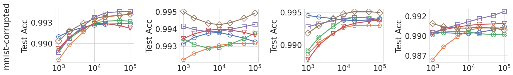
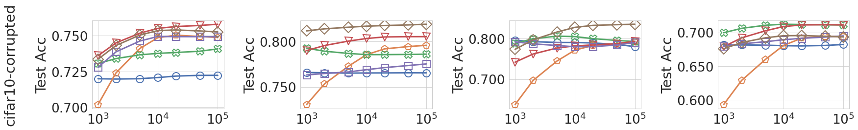
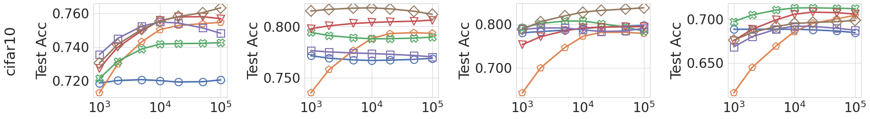
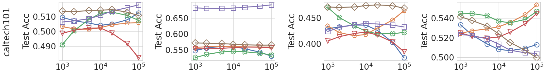
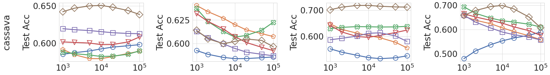
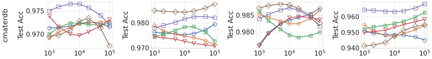
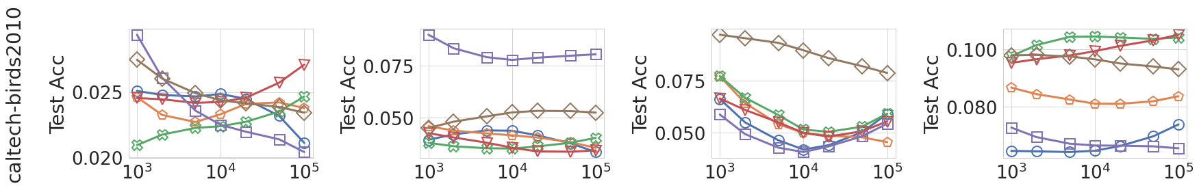
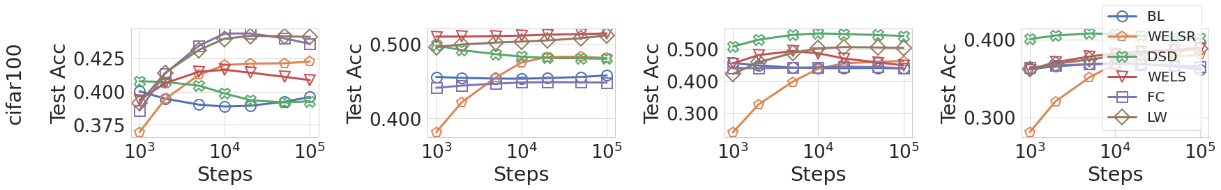
Figure 9: The full version of Figure 4, which contains the full set of datasets.

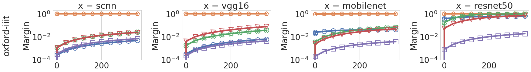
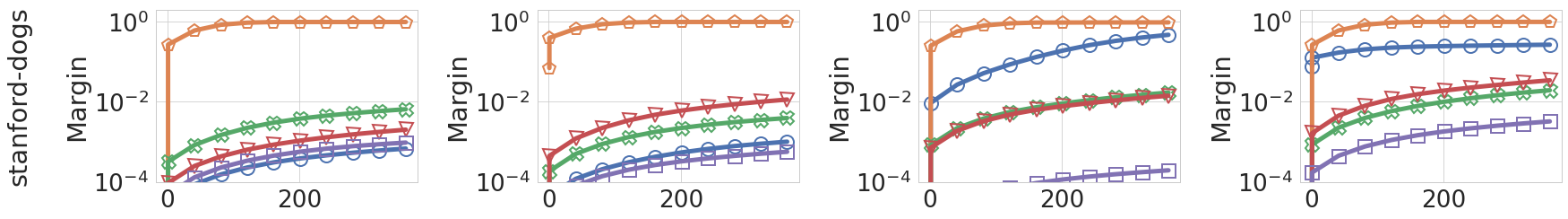
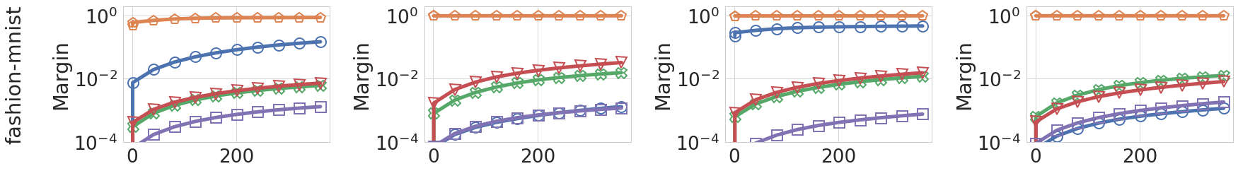
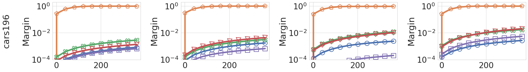
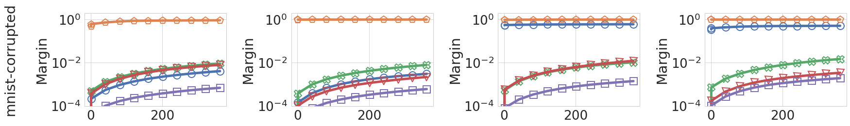
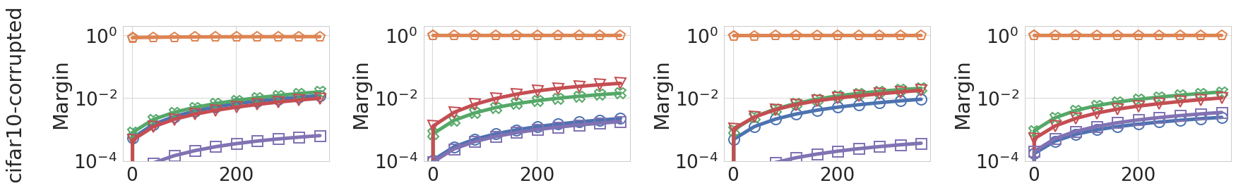
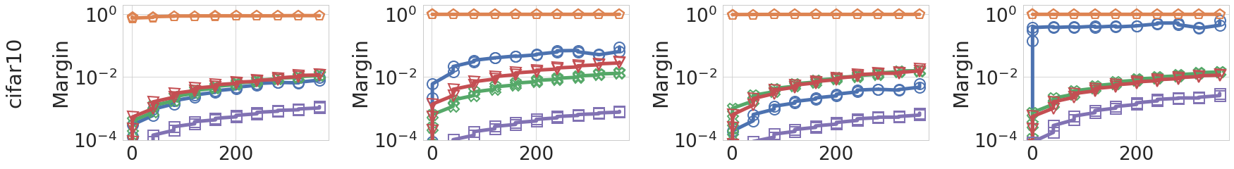
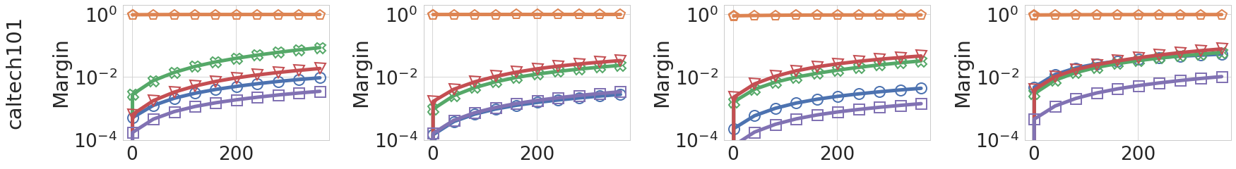
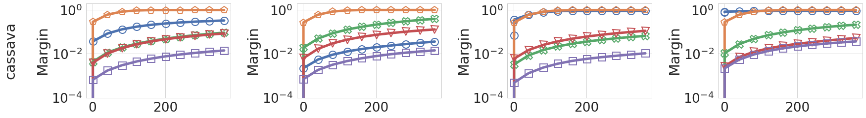
Figure 10: The full version of Figure 6 (top), which contains the full set of datasets.

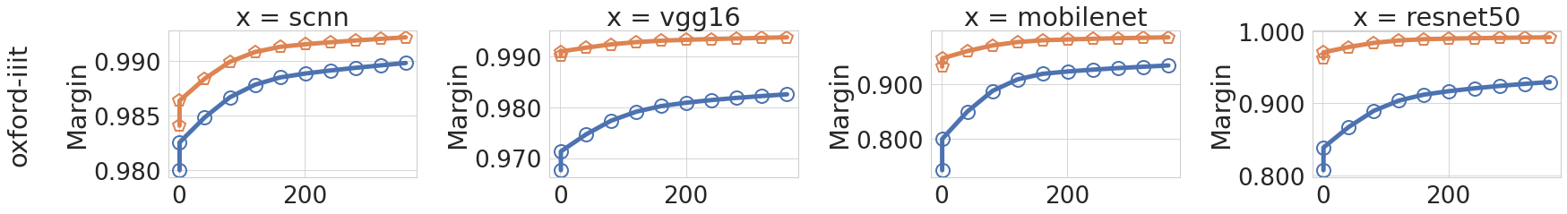
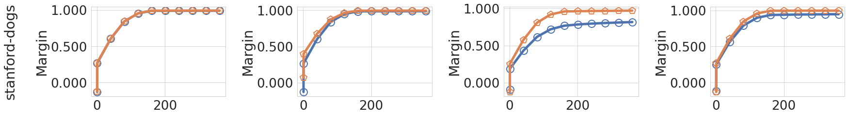
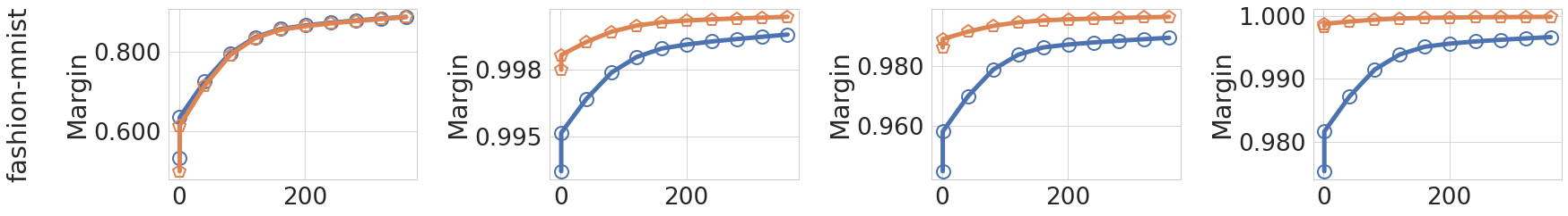
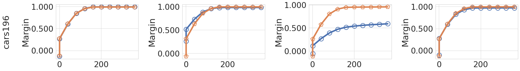
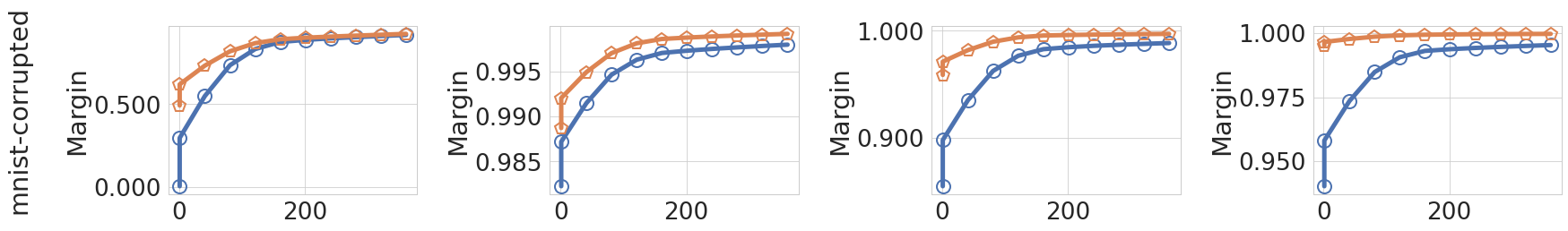
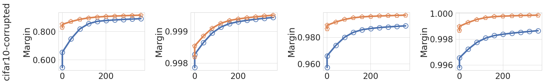
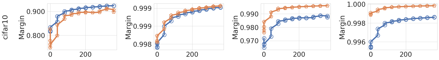
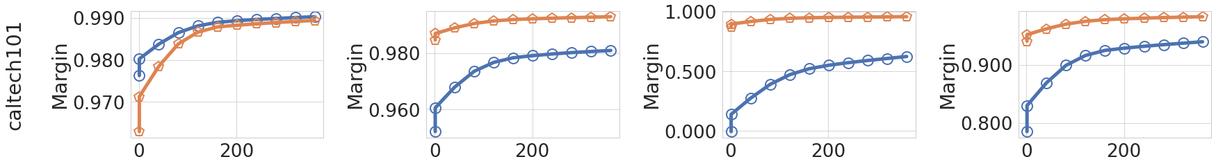
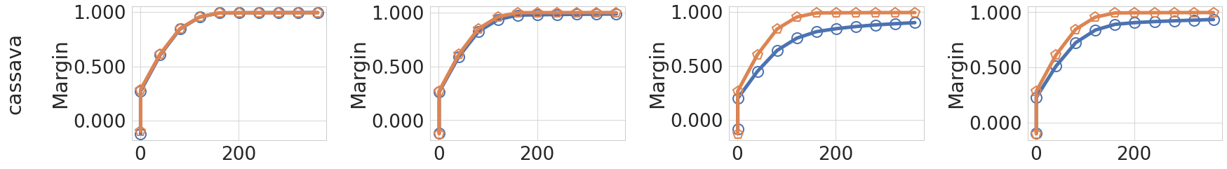
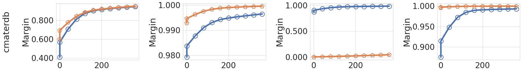
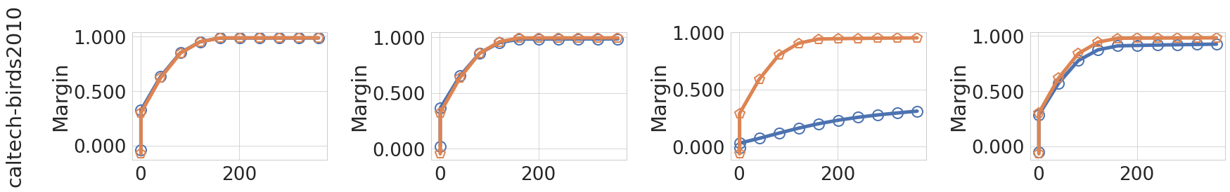
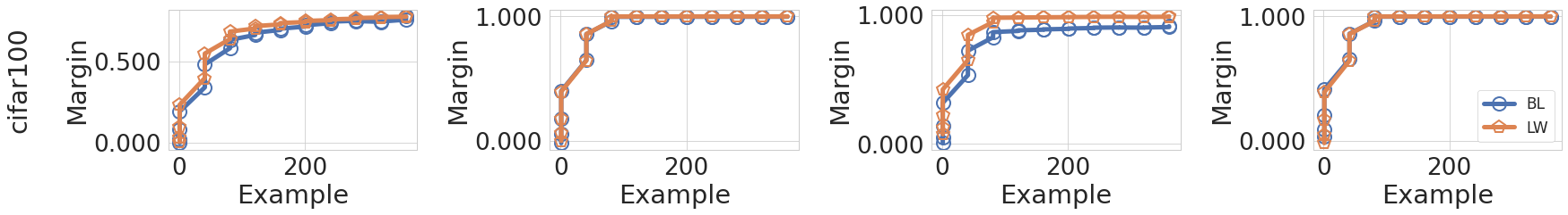
Figure 11: The full version of Figure 6 (bottom), which contains the full set of datasets.

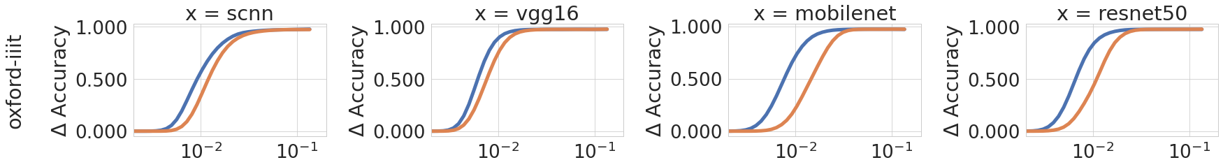
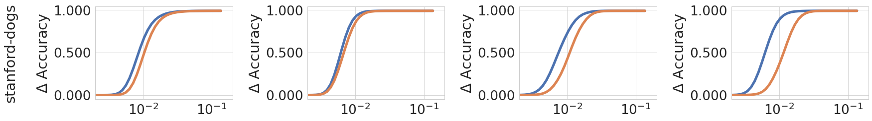
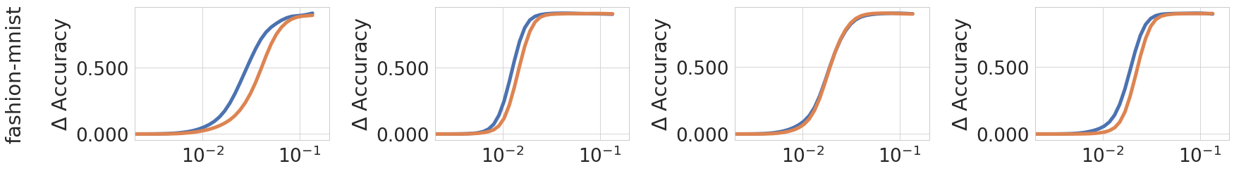
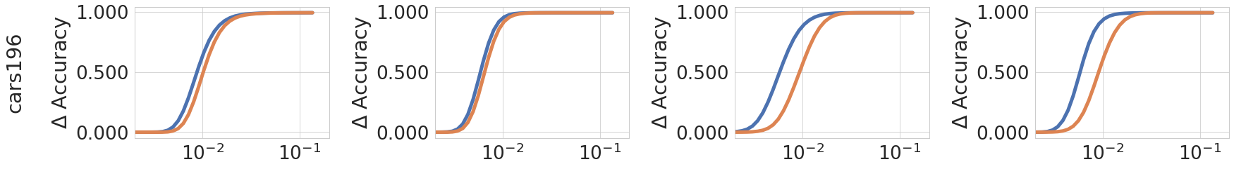
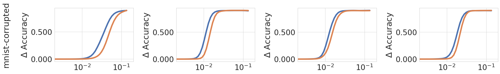
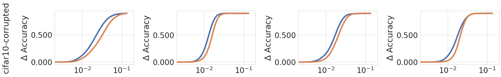
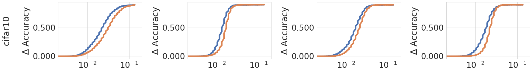
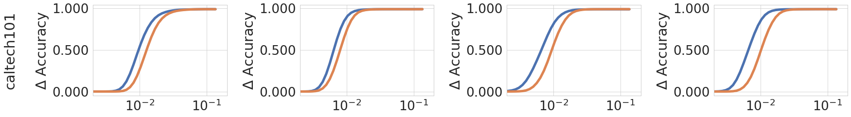
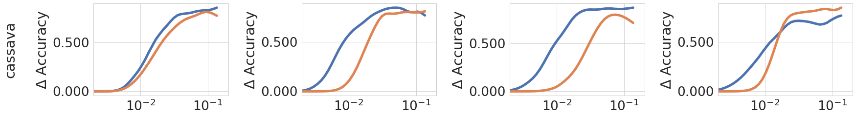
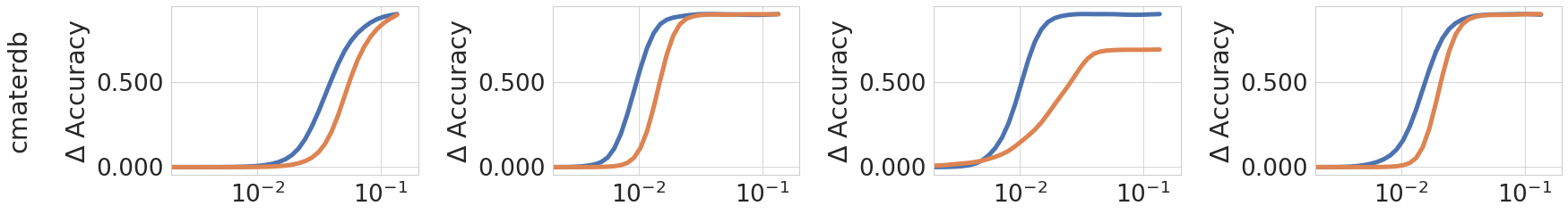
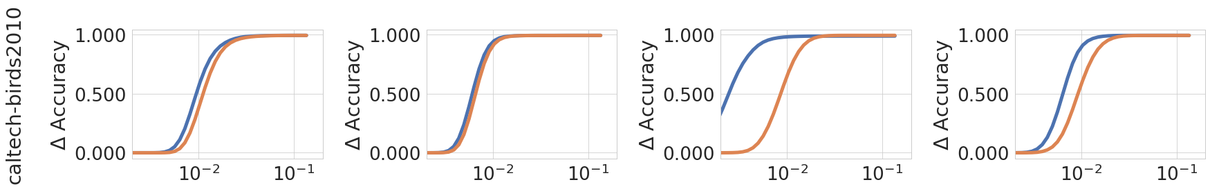
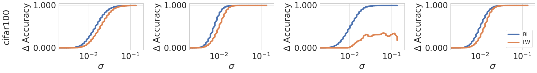
Figure 12: The full version of Figure 5, which contains the full set of datasets.

References

- Abadi et al. (2015) Abadi, M.; Agarwal, A.; Barham, P.; Brevdo, E.; Chen, Z.; Citro, C.; Corrado, G. S.; Davis, A.; Dean, J.; Devin, M.; et al. 2015. TensorFlow: Large-Scale Machine Learning on Heterogeneous Systems. arXiv:1603.04467.
- Arora et al. (2018) Arora, S.; Ge, R.; Neyshabur, B.; and Zhang, Y. 2018. Stronger generalization bounds for deep nets via a compression approach. In ICML.
- Arpit et al. (2017) Arpit, D.; Jastrzkebski, S.; Ballas, N.; Krueger, D.; Bengio, E.; Kanwal, M. S.; Maharaj, T.; Fischer, A.; Courville, A.; Bengio, Y.; and Lacoste-Julien, S. 2017. A closer look at memorization in deep networks. In ICML.
- Ba, Kiros, and Hinton (2016) Ba, J. L.; Kiros, J. R.; and Hinton, G. E. 2016. Layer normalization. In NeurIPS Deep Learning Symposium.
- Baldock, Maennel, and Neyshabur (2021) Baldock, R. J.; Maennel, H.; and Neyshabur, B. 2021. Deep Learning Through the Lens of Example Difficulty. arXiv preprint arXiv:2106.09647.
- Bartlett (1998) Bartlett, P. L. 1998. The sample complexity of pattern classification with neural networks: the size of the weights is more important than the size of the network. IEEE Transactions on Information Theory, 44(2): 525–536.
- Bartlett, Foster, and Telgarsky (2017) Bartlett, P. L.; Foster, D. J.; and Telgarsky, M. J. 2017. Spectrally-normalized margin bounds for neural networks. In NeurIPS.
- Bishop (1995) Bishop, C. M. 1995. Training with noise is equivalent to Tikhonov regularization. Neural computation, 7(1): 108–116.
- Chaudhari et al. (2019) Chaudhari, P.; Choromanska, A.; Soatto, S.; LeCun, Y.; Baldassi, C.; Borgs, C.; Chayes, J.; Sagun, L.; and Zecchina, R. 2019. Entropy-SGD: Biasing gradient descent into wide valleys. Journal of Statistical Mechanics: Theory and Experiment, 2019(12): 124018.
- Cohen, Sapiro, and Giryes (2018) Cohen, G.; Sapiro, G.; and Giryes, R. 2018. DNN or k-NN: That is the Generalize vs. Memorize Question. arXiv:1805.06822.
- Das et al. (2012) Das, N.; Reddy, J. M.; Sarkar, R.; Basu, S.; Kundu, M.; Nasipuri, M.; and Basu, D. K. 2012. A Statistical-topological Feature Combination for Recognition of Handwritten Numerals. Appl. Soft Comput., 12(8): 2486–2495.
- Demšar (2006) Demšar, J. 2006. Statistical comparisons of classifiers over multiple data sets. Journal of Machine Learning Research, 7: 1–30.