Abstract

In this paper we further elaborate on the Bose-Einstein condensate (BEC) dark matter model extended in our preceding work [Phys. Rev. D 2020, 102, 083510] by the inclusion of 6th order (or three-particle) repulsive self-interaction term. Herein, our goal is to complete the picture through adding to the model the 4th order repulsive self-interaction. The results of our analysis confirm the following: while in the preceding work the two-phase structure and the possibility of first-order phase transition was established, here we demonstrate that with the two self-interactions involved, the nontrivial phase structure of the enriched model remains intact. For this to hold, we study the conditions which the parameters of the model, including the interaction parameters, should satisfy. As a by-product and in order to provide some illustration, we obtain the rotation curves and the (bipartite) entanglement entropy for the case of particular dwarf galaxy.

Keywords: dark matter; halo; Bose-Einstein condensate; two- and three-particle self-interactions; two-phase structure; first-order phase transition; dwarf galaxies; rotation curves; entanglement entropy

1 Introduction

Although the concept of dark matter (DM) is a widely accepted one, its precise nature is still escaping. There exist vast multitude of different approaches and models, among which the modeling of DM as Bose-Einstein condensate (BEC), see e.g. [1, 2, 3, 4], the overviews [5, 6] and many others, finds each time more and more support. Positions of BEC model of DM were especially enforced after the works  [7, 8, 9] which demonstrated ability of BEC DM to avoid the core-cusp and the gravitational collapse [10] problems. Also, the model gives quite successful description [7, 11, 12, 13] of the rotation curves of a number of galaxies, at least dwarf and the low surface brightness ones.

Nevertheless, even within this well-elaborated model there also exist some tensions and issues which can be improved. To this end, there is in particular a possibility to apply appropriate tools from the powerful and efficient theory of deformations. Namely, the $\mu$-deformed analog of Bose-gas model developed in [14], with the so-called $\mu$-calculus as a base, has demonstrated clearly the following preferable features: (i) the evaluated mass of DM halo appears more realistic; (ii) the obtained critical temperature of condensation of $\mu$-Bose gas $T^{(\mu)}_{C}$ depends on the deformation parameter $\mu$,  $\mu>0$, and is higher [15] than the usual $T_{C}$; (iii) $\mu$-deformation based description of the rotation curves [16] fits better than the curves inferred within the ordinary BEC model.

It is also worth to mention the recent work [17] which uses the concept of deformed spatial commutation relations for scalar field in order to develop a class of generalization of the Bose-condensate DM model. Such an extension has good potential to achieve improvements.

Another line of extension of the BEC model of DM, developed recently in [18], involves sixth order (or 3-particle) self-interaction term  $\psi^{6}$. Due to presence of the latter, the modified model manifests nontrivial phase structure: there exist two distinct phases, certain region of instability, and the possibility of first-order phase transition.

In order to make the extended model even more complete, it is natural to include, besides the $\psi^{6}$, also the two-particle self-interaction encoded in the term  $\psi^{4}$. Analysis of such “doubly-nonlinear” extension of [18] and BEC model of DM is the goal of the present paper.

The structure of the paper is the following. Necessary details of the model are given in Section 2, and main part that involves obtaining thermodynamic functions and their key properties is presented in Section 3. In Sections 4 and 5 we consider briefly, again for the situation of presence of both two- and three-particle interactions, the rotation curves of selected galaxy and the respective bipartite entanglement entropy of two centrally symmetric regions of the halo of this same galaxy. In our concluding section, we present a discussion of the results.

2 The Model

We describe the Bose-Einstein condensate by real function $\psi(r)$ of radial variable $r=|\mathbf{r}|$, using a constant chemical potential $\tilde{\mu}$. Our study is based on the energy functional $\Gamma$ in a ball $B=\{\mathbf{r}\in\mathbb{R}^{3}|\,|\mathbf{r}|\leq R\}$ and the Poisson equation:

$$\Gamma=4\pi\int_{0}^{R}\left[\frac{\hbar^{2}}{2m}(\partial_{r}\psi(r))^{2}+m\psi^{2}(r)V_{\mathrm{gr}}(r)+\frac{U_{2}}{2}\psi^{4}(r)+\frac{U_{3}}{3}\psi^{6}(r)-\tilde{\mu}\psi^{2}(r)\right]\,r^{2}\,\mathrm{d}r,$$ (1)

$$\Delta_{r}V_{\mathrm{gr}}(r)=4\pi Gm|\psi(r)|^{2},$$ (2)

where $\Delta_{r}$ is the radial part of Laplace operator that acts as

$$\Delta_{r}f(r)=\partial^{2}_{r}f(r)+\frac{2}{r}\,\partial_{r}f(r),$$ (3)

$$\Delta^{-1}_{r}f(r)=-\frac{1}{r}\int_{0}^{r}f(s)\,s^{2}\,\mathrm{d}s-\int_{r}^{R}f(s)\,s\,\mathrm{d}s,$$ (4)

$R$ being the radius of the ball where the matter is located.

Focusing here on the effects of interparticle interactions, we leave aside the slow rotation of the condensate [13], which can be taken into account through the chemical potential [17].

For convenience, let us introduce dimensionless variables:

$$\psi(r)=\sqrt{\varrho_{0}}\,\chi(\xi),\quad r=r_{0}\,\xi,\quad u=\tilde{\mu}\,\frac{mr_{0}^{2}}{\hbar^{2}},$$

$$A=4\pi\frac{Gm^{3}\varrho_{0}r_{0}^{4}}{\hbar^{2}},\quad Q=U_{2}\frac{\varrho_{0}mr_{0}^{2}}{\hbar^{2}},\quad B=U_{3}\frac{\varrho_{0}^{2}mr_{0}^{2}}{\hbar^{2}}.$$ (5)

Here $\chi(\xi)$ is a real dimensionless scalar field; $\varrho_{0}$ and $r_{0}$ characterize typical measures of the central particle density and the system size, respectively.

Thus, we arrive at

$$\frac{\Gamma}{\Gamma_{0}}=\int_{0}^{\xi_{B}}\left[\frac{1}{2}(\partial_{\xi}\chi)^{2}-u\chi^{2}+A\chi^{2}\varphi+\frac{Q}{2}\chi^{4}+\frac{B}{3}\chi^{6}\right]\xi^{2}\,\mathrm{d}\xi,\quad\Gamma_{0}=\frac{4\pi\hbar^{2}r_{0}\varrho_{0}}{m},$$

$$\Delta_{\xi}\varphi(\xi)=\chi^{2}(\xi),$$ (6)

where $\xi_{B}=R/r_{0}$, whereas $\Delta_{\xi}$ and $\Delta^{-1}_{\xi}$ are given by (3), (4) in terms of $\xi$ replacing $r$.

To estimate the range of parameter values, we turn to astrophysical situations. Since we suggest to take into account the three-particle interaction in relatively dense DM of light bosons with masses of the order of $10^{-22}\ \mathrm{eV}\,c^{-2}$, ranges of the parameters can be found by considering the DM of galactic cores with a central mass density $\rho_{0}=m\varrho_{0}$ of the order of $10^{-20}\ \mathrm{kg}\,\mathrm{m}^{-3}$, in the region of radius $r_{0}$ smaller than 1 kpc. Then, extracting $r_{0}$ from the definition (5) of the measure of gravitational interaction $A$,

$$r_{0}\simeq 0.824\ \mathrm{kpc}\,\left[\frac{A}{10}\right]^{1/4}\,\left[\frac{mc^{2}}{10^{-22}\ \mathrm{eV}}\right]^{-1/2}\,\left[\frac{\rho_{0}}{10^{-20}\ \mathrm{kg}\,\mathrm{m}^{-3}}\right]^{-1/4},$$ (7)

we can adopt that $A\sim 10$ [18].

It is clear that the gravity results from integral effect of a whole system. Unlike, (thermo)dynamics of internal processes is determined by repulsive interactions among bosons, represented by the parameters $Q$ and $B$ under the condition $B>A$. The role of pairwise interaction, controlled by $Q$, is assumed to be comparable with the effect of gravity.

Using (7), the characteristic energy density $\varepsilon_{0}=\hbar^{2}\varrho_{0}/(mr^{2}_{0})$ is evaluated as

$$\varepsilon_{0}\simeq 33.82\ \mathrm{eV}\,\mathrm{cm}^{-3}\,\left[\frac{A}{10}\right]^{-1/2}\,\left[\frac{mc^{2}}{10^{-22}\ \mathrm{eV}}\right]^{-1}\,\left[\frac{\rho_{0}}{10^{-20}\ \mathrm{kg}\,\mathrm{m}^{-3}}\right]^{3/2}.$$ (8)

In the pressure units, $33.82\ \mathrm{eV}\,\mathrm{cm}^{-3}\simeq 5.42\cdot 10^{-12}\ \mathrm{Pa}$.

Extremizing of functional $\Gamma$, i.e. $\delta\Gamma/\delta\chi(\xi)=0$, yields the set of field equations:

$$\frac{1}{2}\Delta_{\xi}\chi+u\chi-A\chi\varphi-Q\chi^{3}-B\chi^{5}=0,\hskip 25.0pt\Delta_{\xi}\varphi=\chi^{2}.$$ (9)

We combine the model equations in the spirit of [18] by introducing the field $\upsilon(\xi)$:

$$\upsilon(\xi)=\int_{0}^{\xi}\chi^{2}(s)\,s\,\mathrm{d}s,\hskip 25.0pt\upsilon(\xi_{B})=-\varphi(0).$$ (10)

As result,

$$2\frac{\Gamma}{\Gamma_{0}}=\int_{0}^{\xi_{B}}\left[(\partial_{\xi}\chi)^{2}-u_{*}\,\chi^{2}(\xi)+\frac{Q_{*}}{2}\,\chi^{4}(\xi)+\frac{B_{*}}{3}\,\chi^{6}(\xi)\right]\,\xi^{2}\,\mathrm{d}\xi$$

$$\hskip 28.45274pt-\frac{A_{*}}{2}\int_{0}^{\xi_{B}}[\upsilon(\xi_{B})-\upsilon(\xi)]^{2}\,\mathrm{d}\xi,$$ (11)

$$\Delta_{\xi}\chi+\nu\chi-\chi\frac{A_{*}}{\xi}\int_{0}^{\xi}\upsilon(s)\,\mathrm{d}s-Q_{*}\chi^{3}-B_{*}\chi^{5}=0,$$ (12)

$$\partial_{\xi}\upsilon(\xi)=\xi\,\chi^{2}(\xi),\hskip 25.0pt\upsilon(0)=0,$$ (13)

$$\nu=A_{*}\upsilon(\xi_{B})+u_{*},$$ (14)

where $A_{*}=2A$, $Q_{*}=2Q$, $B_{*}=2B$, and $\nu$ (put instead of $u_{*}=2u$) are arbitrary positive parameters. The system boundary $\xi_{B}$ is defined from the condition $\chi(\xi_{B})=0$ and is the first zero of oscillating function $\chi(\xi)$.

In order to find a decreasing solution $\chi(\xi)$ for admissible $\xi$ with a finite initial value $\chi_{0}=\chi(0)<\infty$, we first impose $\chi^{\prime}(0)=0$ and then formulate the conditions which allow to fix $\chi_{0}$, through expanding $\chi(\xi)=\chi_{0}+C_{2}\xi^{2}+\dots$ at $\xi\to 0$. On substituting that in (12), (13), the following algebraic equations result:

$$6C_{2}+\nu\chi_{0}-Q_{*}\chi^{3}-B_{*}\chi^{5}_{0}=0,$$

$$\nu C_{2}-\frac{A_{*}}{6}\,\chi^{3}_{0}-3Q_{*}\chi^{2}_{0}C_{2}-5B_{*}\chi^{4}_{0}C_{2}=0.$$ (15)

Combining the two, we find that the value $\chi_{0}$ should satisfy the equation $S(A_{*},B_{*},Q_{*},\nu,\chi_{0})=0$, where

$$S(A_{*},B_{*},Q_{*},\nu,z)=A_{*}z^{2}-(5B_{*}z^{4}+3Q_{*}z^{2}-\nu)(\nu-Q_{*}z^{2}-B_{*}z^{4}),$$ (16)

plus the condition $2C_{2}=\chi^{\prime\prime}(0)\leq 0$. Taken altogether, these constrain $\chi_{0}$ as $z_{1}<\chi_{0}<z_{2}$, where

$$z_{1}=\left[\sqrt{\left(\frac{3Q_{*}}{10B_{*}}\right)^{2}+\frac{\nu}{5B_{*}}}-\frac{3Q_{*}}{10B_{*}}\right]^{1/2},\quad z_{2}=\left[\sqrt{\left(\frac{Q_{*}}{2B_{*}}\right)^{2}+\frac{\nu}{B_{*}}}-\frac{Q_{*}}{2B_{*}}\right]^{1/2}.$$ (17)

Technically, the search for the initial value $\chi_{0}$ of the model which takes into account the pair interaction is similar to the problem with three-particle interaction only [18]. Likewise, we notice three regimes (for given $A_{*}$, $Q_{*}$, $B_{*}$ and $\nu$): 1) no solution for $\chi_{0}$ that, in Eq. (12), leads to $\chi(\xi)=0$; 2) single solution $\chi_{0}$ that corresponds to a minimal admissible value $\nu_{\mathrm{min}}$ from which the system starts to evolve; 3) pair of (positive) solutions for $\chi_{0}$, when we should choose a minimal one, because the other leads to divergent $\chi(\xi)$. Usually, for fixed $(A_{*},Q_{*},B_{*})$, but increasing $\nu$, the indicated sequence of all three options occurs.

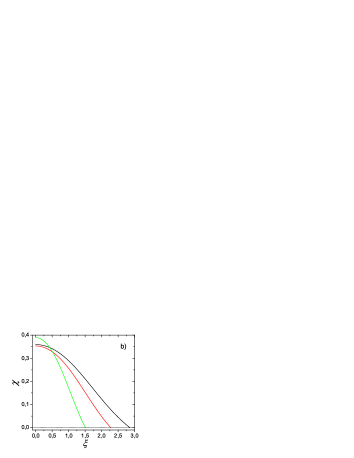
It is useful to analyze the system from the quantum-mechanical point of view. Equation (12) for $\xi\leq\xi_{B}$ can be conveniently rewritten in the Schrödinger form to describe the scattering of a particle whose wave function is taken as $f(\xi)=c\chi(\xi)$ ($c$ is a normalization depended on a total number of particles) in the potential $V_{\mathrm{eff}}$:

$$\left(-\frac{1}{2}\Delta_{\xi}+V_{\mathrm{eff}}(\xi)\right)f(\xi)=uf(\xi),$$ (18)

$$V_{\mathrm{eff}}(\xi)=V_{2}(\xi)+V_{3}(\xi),$$ (19)

$$V_{2}(\xi)=Q\chi^{2}(\xi)+V_{\mathrm{gr}}(\xi),\quad V_{3}(\xi)=B\chi^{4}(\xi),$$ (20)

$$V_{\mathrm{gr}}(\xi)=-A\upsilon(\xi_{B})+\frac{A}{\xi}\int_{0}^{\xi}\upsilon(s)\mathrm{d}s,$$ (21)

where potentials $V_{2}$ and $V_{3}$ come from two and three-particle interactions, respectively. Substituting the found solution $\chi(\xi)$, we can see that the form of potential $V_{\mathrm{eff}}$ depends also on a chemical potential $u$ (or parameter $\nu$).

Figure 1: a) The effective potential $V_{\mathrm{eff}}(\xi)$ for $u_{\mathrm{black}}\simeq 0.149$, $u_{\mathrm{red}}\simeq-0.502$, $u_{\mathrm{green}}\simeq-2.046$. Dashed parts of the curves correspond to a pure gravitational potential $-A\cdot{\cal N}/\xi$ outside the particle system. b) The field $\chi(\xi)$ for the same values of chemical potential $u$, and $\chi(\xi)=0$ at $\xi=\xi_{B}$. Here $A=10$, $B=20$, $Q=1.36$ for definiteness.

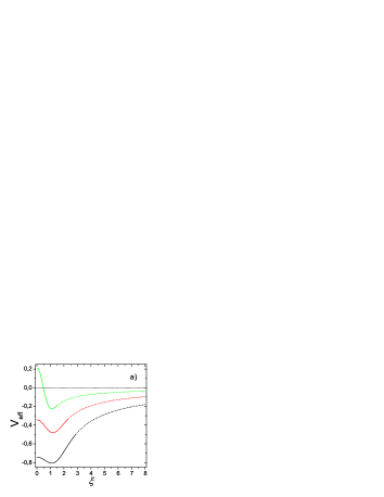
In Fig. 1 we have used the values $A=10$, $B=20$ and $Q=1.36$. The latter one plays the role of “critical” value (its sense is seen in Fig. 2 below, with explanations at the end of the next Section). We relate the particular forms of $V_{\mathrm{eff}}$ given in Fig. 1a with the physical situations depicted in Fig. 2 below. Namely, green curve in Fig. 1a is chosen for liquid-like (dense) state in Fig. 2, when the three-particle interaction contributes to a hard-core part of potential at small $\xi$. Red curve is constructed in the vicinity of the critical point of the first-order phase transition, when the potential $V_{\mathrm{eff}}$ is similar to the harmonic trap. Black curve corresponds to gaseous (dilute) state in the effective (truncated) gravitational potential, when the kinetic energy term dominates ($u>0$).

In the range $\xi\geq\xi_{B}$ we come to the problem of a particle in the gravitational field (see the dashed curves in Fig. 1a) created by the system of ${\cal N}$ particles:

$$\left(-\frac{1}{2}\Delta_{\xi}-A\frac{{\cal N}}{\xi}\right)f_{k}(\xi)=\frac{k^{2}}{2}f_{k}(\xi),\quad f_{k}(\xi_{B})=0,\quad f^{\prime}_{k}(\xi_{B})=f^{\prime}(\xi_{B}),$$ (22)

where

$${\cal N}=\int_{0}^{\xi_{B}}\chi^{2}(\xi)\,\xi^{2}\mathrm{d}\xi$$ (23)

is the total number of particles within the ball $\xi\leq\xi_{B}$, which determines the total mass.

At this stage a wave number $k$ is ambiguous. Oscillating and decaying solution to this equation (for any real $k$ and pure imaginary $\kappa$ and $s$) is given as:

$$f_{k}(\xi)=\frac{c_{1}M_{s,1/2}(\kappa\xi)+c_{2}W_{s,1/2}(\kappa\xi)}{\xi},\quad\kappa=2\mathrm{i}k,\quad s=\frac{2A{\cal N}}{\kappa},$$ (24)

$$c_{1}=f^{\prime}(\xi_{B})\,\xi^{2}_{B}\,\frac{W_{s,1/2}(\kappa\xi_{B})}{F(\kappa)},\hskip 25.0ptc_{2}=-f^{\prime}(\xi_{B})\,\xi^{2}_{B}\,\frac{M_{s,1/2}(\kappa\xi_{B})}{F(\kappa)},$$ (25)

$$F(\kappa)=(1+s)M_{1+s,1/2}(\kappa\xi_{B})\,W_{s,1/2}(\kappa\xi_{B})+M_{s,1/2}(\kappa\xi_{B})\,W_{1+s,1/2}(\kappa\xi_{B}).$$ (26)

Here $M_{\mu,\nu}(z)$ and $W_{\mu,\nu}(z)$ are the Whittaker functions.

This solution might be interpreted as the gravitational capture of a dark matter particle (a radial wave with energy $k^{2}/2$) outside the dark matter ball, when $\xi\to\infty$. In the case of initially resting particle with $k=0$, the solution is described in terms of Bessel functions $J_{1}(z)$ and $Y_{1}(z)$.

Thus, the account of interaction confirms the possibility of bound states, which can manifest themselves in the form of different thermodynamic phases. Further, all global quantities of the model, computed at fixed $A$, $Q$ and $B$, are supposed to be functions of free parameter $\nu$. Therefore, dependence, say, of $a$ on $b$ should be treated in parametric form: $a(b)=\{(b(\nu),a(\nu))|\nu\geq\nu_{\mathrm{min}}\}$.

3 Thermodynamic Quantities and Two Phases

To study the macroscopic properties, let us define an effective chemical potential $\mu(\xi)$ [19], which includes the gravitational potential jointly with the term of quantum fluctuations, and replaces further the constant chemical potential $u$, that is

$$\mu(\xi)+A\varphi(\xi)-\frac{1}{2\chi(\xi)}\Delta_{\xi}\chi(\xi)=u.$$ (27)

Accordingly to the equation of motion (9), $\mu$ determines $\chi$ as

$$\mu(\xi)=Q\chi^{2}(\xi)+B\chi^{4}(\xi),\hskip 25.0pt\mu(\xi_{B})=0.$$ (28)

For finding macroscopic characteristics, we appeal to the thermodynamic relations at $T=0$, using a local particle density $\eta(\xi)=\chi^{2}(\xi)$:

$$\mathrm{d}p(\xi) = \eta(\xi)\,\mathrm{d}\mu(\xi),\hskip 48.93872ptp(\xi_{B})=0,$$ (29)

$$\varepsilon(\xi) = \eta(\xi)\,\mu(\xi)-p(\xi),\hskip 25.0pt\varepsilon(\xi_{B})=0,$$ (30)

where functions $p(\xi)$ and $\varepsilon(\xi)$ determine the (dimensionless) mean pressure $P$ and the internal energy $E$:

$$P=\frac{3}{\xi^{3}_{B}}\int_{0}^{\xi_{B}}p(\xi)\,\xi^{2}\,\mathrm{d}\xi,\hskip 25.0ptE=\int_{0}^{\xi_{B}}\varepsilon(\xi)\,\xi^{2}\,\mathrm{d}\xi.$$ (31)

Hereafter, $\xi^{3}_{B}/3$ represents the volume of the system.

Therefore, we need to integrate the Gibbs–Duhem relation (29) and then to substitute $p(\xi)$ into the Euler relation (30) in order to find $\varepsilon(\xi)$. This way, the explicit expressions are obtained:

$$p(\xi)=\frac{Q}{2}\eta^{2}(\xi)+\frac{2}{3}B\eta^{3}(\xi),\hskip 25.0pt\varepsilon(\xi)=\frac{Q}{2}\eta^{2}(\xi)+\frac{1}{3}B\eta^{3}(\xi),$$ (32)

which give us the equation of state by inserting the solution $\eta(\xi)$ of (12)–(14).

The (local) internal pressure $p(\xi)$ behaves spatially with radius accoding to

$$\frac{\partial_{\xi}p(\xi)}{\eta(\xi)}=\partial_{\xi}\mu_{q}(\xi)=-A\frac{n(\xi)}{\xi^{2}}+\partial_{\xi}\left(\frac{1}{2\chi(\xi)}\Delta_{\xi}\chi(\xi)\right),\quad n(\xi)=\int_{0}^{\xi}\eta(s)\,s^{2}\,\mathrm{d}s.$$ (33)

We do not solve it because all necessary fields are found explicitly from Eqs. (12)–(14).

Mean particle density is

$$\sigma=\frac{3}{\xi^{3}_{B}}\int_{0}^{\xi_{B}}\chi^{2}(\xi)\,\xi^{2}\mathrm{d}\xi.$$ (34)

Figure 2: Equation of state of dark matter at $T=0$ and fixed parameters $A$ and $B$. A slow growth in dimensionless pressure $P$ at relatively low density $\sigma$ corresponds to a dilute phase of matter, while a steep rise indicates a denser liquidlike phase at high densities. Orange curve (with two extrema) demonstrates the presence of metastable states. Black line is for a critical value of $Q_{c}=1.36$. Green line exemplifies a continuous transition between the two phases at $Q<Q_{c}$.

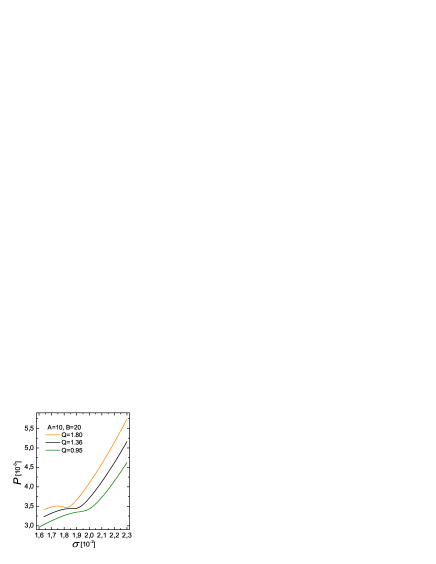
Dependence of mean internal pressure $P$, see (31), on this density $\sigma$ is presented in Fig. 2 for various parameters of interaction. The curves obtained numerically reveal the presence of two stable phases of dark matter with $\partial P/\partial\sigma>0$: the dilute one ($\partial^{2}P/\partial\sigma^{2}<0$) and the denser liquidlike one ($\partial^{2}P/\partial\sigma^{2}>0$). The characteristic points of the phase diagram are determined from the conditions: $\partial P/\partial\sigma=0$ and $\partial^{2}P/\partial\sigma^{2}=0$. The simultaneous fulfillment of these conditions at a single point determines the critical point, which belongs to the black curve in Fig. 2, and inferring of which is one of main tasks here. The existence of a critical point of a first-order phase transition is essentially related to the competition between gravitational and pair interactions, controlled by the parameter $Q$.

While the presence of metastable states, linked with the two-extrema behavior at $Q>1.36$ and shown by the orange curve, clearly indicates mixing of the gaseous and liquid phases, a detailed description of the transition between the two phases at $Q<1.36$ requires the use of additional thermodynamic characteristics, as is already done in [18] by means of the perturbation pressure $\Pi_{\nu}$ for $Q=0$.

It is important to emphasize that herein we reveal a discontinuous behavior (jump between two phases) of the density $\sigma$ with the change in the internal pressure $P$. The existence of such a regime, as we show, is allowed at $Q>1.36$ for $A=10$ and $B=20$. Although the existence of a denser, liquidlike phase of DM (in a relatively small region of halo) is possible at $Q=0$, the condition $Q>0$ is required in describing the galactic DM halos [7], even without taking into account the three-particle interaction.

Note that a continuous change in the parameter $Q$ can lead to the intersection of different curves $P(\sigma)$, that indicates the possibility of realizing one thermodynamic state by fixation of different sets of parameters. Such ambiguity in the set of parameters can complicate the interpretation and reproduction of observables.

4 The Rotation Curves

Important information about dark matter is extracted and verified from the rotation curves of galaxies. As our model is aimed to study the processes in dark matter in the galaxy cores, that is, in relatively small regions of space with a noticeable density, its direct application to the description of rotation curves should be limited to dwarf galaxies (or other dark matter dominated compact galaxies). One of the possibilities for describing larger (halo-type) objects is to extend the model, similarly to what was proposed in [18]. Besides, the lack of accounting for the rigid rotation of matter in the model does not allow us to describe the curves of rotating galaxies. Nevertheless, we consider it important and interesting to demonstrate the capabilities of our model, in which we accurately took into account quantum fluctuations in the condensate and (both two- and) three-particle interactions. Although the extensions of the model are indicated in [18, 17], the included effects make it possible to further validate the Bose-condensate approach, to compare with and supplement the results of [7].

Thus, the tangential velocity $v$ of a test particle moving in the spherically symmetric DM halo can be represented as

$$v(r)=\sqrt{G\frac{M(r)}{r}},\hskip 25.0ptM(r)=4\pi\int_{0}^{r}\rho(s)\,s^{2}\,\mathrm{d}s,$$ (35)

where $\rho(r)=m|\psi(r)|^{2}$ is a mass density such that $\rho(R)=0$ at $R=r_{0}\xi_{B}$.

Figure 3: Rotation curves for dwarf galaxy M81dwB with mass $M=3\cdot 10^{8}M_{\odot}$. Blue dots are the observed data for $r\leq 1~{}\text{kpc}$. Solid lines are obtained within the model under certain restrictions: cyan line is for $M^{(1)}_{\rm BEC}=3\cdot 10^{8}M_{\odot}$ and $R^{(1)}=1~{}\text{kpc}$; black line is for $M^{(2)}_{\rm BEC}=3\cdot 10^{8}M_{\odot}$ and $R^{(2)}\simeq 1.12~{}\text{kpc}$; orange line corresponds to $M^{(3)}_{\rm BEC}=3.5\cdot 10^{8}M_{\odot}$ and $R^{(3)}=1.3~{}\text{kpc}$.

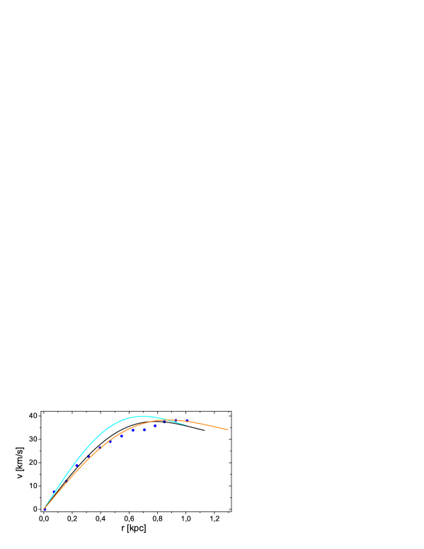
Let us illustrate the model predictions for the rotation curves of the M81 galaxy, shown in Fig. 3. Note especially the free parameters of the model $A$, $B$, $Q$, $\nu$, $\rho_{0}$ that we use for fitting, as well as the restricting characteristics: the total mass $M$ of dark matter and the halo radius $R$.

The galaxy M81 with no rigid rotation gives us the most striking proof of the Bose-condensate approach, as noted in [7]. Let us use this example to emphasize main features of the description of rotation curves.

First of all, note it looks rather difficult to indicate unambiguously the parameters for the rotation curve: the same dependence $v(r)$ can be realized for different sets of the parameters. This is a consequence of the symmetry of the model equations. For this reason, we give only graphs that are interesting for physics, and omit the mathematics of identifying the symmetries.

In our example, it is worth to note a possibility to construct the curve colored in cyan in Fig. 3 with $Q=0$, when the pair interaction is absent. At the same time, the best fitted dependencies, represented by other curves, always require $Q>0$. This implies that the repulsive pair interaction should be taken into account in realistic models of dark matter in (dwarf) galaxies [11, 20].

5 Entanglement Entropy

The possibility of estimating the entanglement entropy in a general Bose condensate was developed, in particular, in [21]. The idea of using this entropy as a criterion for differentiating the BEC dark matter from cold dark matter (CDM) was proposed in [22]. Although a more precise analysis requires studying the effects of interference of particles from interacting subsystems, here we estimate the entropy between two separated (central and surrounding) parts of radially inhomogeneous BEC dark matter of a galaxy. Omitting the normalization constants, we use the formula (in accordance with [21, 22]):

$$S_{E}(x)=\ln{\{c(x\xi_{B})\,[1-c(x\xi_{B})]\}},\hskip 25.0ptx=\xi/\xi_{B}=r/R.$$ (36)

Here $c(\xi)=n(\xi)/{\cal N}$ is the fraction of particles contained in the central subsystem, $n(\xi)$ being defined in (33).

Figure 4: Entanglement entropy $S_{E}$ within the model with $A=10$, $B=20$, $Q=1.36$ and $u\simeq-2.046$.

A typical dependence of the entanglement entropy on the specific radius is shown in Fig. 4. It is worth noting that, although the system is inhomogeneous, and $c(\xi)$ is not a constant, the maximum influence of one subsystem of particles upon the other turns out to occur at $x=0.5$. What concerns negative sign of $S_{E}(x)$: that is eliminated by explicit account of normalization constant, that is, by adding definite positive number (of the order $10^{2}$ or higher, see e.g. [22]) which depends on the mass of dark matter particles and their number in the subregion.

6 Discussion

In the framework of the extended version of BEC dark matter model that involves two- and three-particle interactions we explored the solutions of the system of equations (11)-(14) as well as the properties of thermodynamic functions. The analysis has led us to the conclusions that the interplay of the basic free parameters $A$, $Q$ and $B$ gives interesting consequences for the system under study including dark matter halo properties: (i) first, the effective interaction potential, see (18)-(21) and Fig. 1, and the density profiles; (ii) the equation of state which shows basic dependence on the parameter $Q$ including existence of its “critical” value $Q_{C}$ that separates different regimes; (iii) persistence at $Q>Q_{C}$ of nontrivial phase structure (inherited from the restricted pure $\psi^{6}$ sub-model). The obtained information on the thermodynamic function such as the mass density profile, enabled us to infer in Sec. 3 the galactic rotation curves, and the bipartite entanglement entropy in Sec. 4. The former clearly demonstrated, with the example of dwarf galaxy M81, that the model can easily provide nice agreement with observational data. As follows from the treatment of rotational curves, the parameter $Q$ responsible for the two-particle interaction plays essential role. Besides, as seen in Fig. 2, at $Q>Q_{C}$ the model reveals the most rich behavior: the curves possess two extrema that implies the metastability region. At $Q\geq Q_{C}$, only inflection points do survive. Without $Q$ (without pair interaction) we could not have such features of unexpected behavior. Anyway, for both $Q>0$ and $Q=0$ (that brings us back to the situation explored in [18]) the two phases are present, though their identification involves differing thermodynamical functions.

It is of interest to compare the model considered in this paper with some of the nonlinear (namely, non-polynomial) extensions of the BEC model of DM, e.g. those studied in [23, 24, 25, 26] where the scalar potential $V_{0}[\cosh\left(\lambda\kappa\Phi\right)-1]$ was employed, with $\kappa=\sqrt{8\pi G}$. The essential feature of these models is the presence of all-order nonlinearities, with the corresponding powers of the single free parameter $\lambda$ (note that $\lambda$ can be viewed as a deformation parameter since at $\lambda\to 0$ the potential and thus the interaction are vanishing). On one hand, the model studied above is obviously simpler than the models involving $\cosh$ or $\cos$: indeed, we encounter the first terms of series expansion if the parameters are restricted as $A=\sqrt{B}=\lambda$. On the other hand, the $\sim\!\psi^{4}$ plus $\sim\!\psi^{6}$ model studied herein is richer in the sense that it operates with the free parameters $A,\ {B},\ Q$, instead of single one. It is this property that allowed us to disclose (confirm) the existence of two phases and of the phase transition. Moreover, the influence of different values of these parameters was essential in our treatment of the rotation curves and the entanglement entropy, see Fig. 4 above.

Concerning the entanglement, an interesting question arises for the situation when dark matter particles are not elementary bosons, but composites built from two bosons or two fermions. In the both cases (i) the composites differ from pure bosons and are naturally realizable, as can be seen in [27], through deformed oscillators or deformed bosons (or quasi-bosons); (ii) bipartite internal entanglement entropy of quasibosons obtained in [28, 29] turned out to depend on the deformation parameter. The question now is as follows: to which extent the microscopic intra-quasibosonic entanglement and its entropy do affect (superimpose with) the macroscopic entanglement and the entanglement entropy that was studied in Sec. 5 above. Also it is no doubt important to explore in detail the connection [21, 30, 31, 32] between peculiarities of the behavior of entanglement and the phase transition (of the first order in our case), especially in the context of the properties of dark matter. We hope to explore these questions in one of our future works.

References

- [1] Sin, S.-J. Late-time phase transition and the galactic halo as a Bose liquid. Phys. Rev. D 1994, 50, 3650.
- [2] Lee, J.-W.; Koh, I.-G. Galactic halos as boson stars. Phys. Rev. D 1996, 53, 2236.
- [3] Hu, W.; Barkana, R.; Gruzinov, A. Fuzzy cold dark matter: the wave properties of ultralight particles. Phys. Rev. Lett. 2000, 85, 1158.
- [4] Bohmer, C.G.; Harko, T. Can Dark Matter Be a Bose-Einstein Condensate? J. Cosmol. Astropart. Phys. 2007, 06, 025.
- [5] Suarez, A.; Roblez, V.; Matos, T. A review on the scalar field/Bose-Einstein condensate Dark Matter. Astrophys. Space Sci. Proc. 2014, 38, 107.
- [6] Fan, J.J. Ultralight Repulsive Dark Matter and BEC. Physics of the Dark Universe 2016, 14, 84-94.
- [7] Harko, T. Bose-Einstein condensation of dark matter solves the core/cusp problem. J. Cosmol. Astropart. Phys. 2011, 05, 022.
- [8] Deng, H.; Hertzberg, M.P.; Namjoo, M.H.; Masoumi, A. Can Light Dark Matter Solve the Core-Cusp Problem? Phys. Rev. D 2018, 98, 023513.
- [9] Harko, T. Jeans instability and turbulent gravitational collapse of Bose–Einstein condensate dark matter halos. Eur. Phys. J. C 2019, 79, 787.
- [10] Khlopov, M.Yu.; Malomed, B.A.; Zeldovich, Ya.B. Gravitational instability of scalar fields and formation of primordial black holes. Mon. Not. R. Astron. Soc. 1985, 215, 575-589.
- [11] Craciun, M.; Harko, T. Testing Bose-Einstein condensate dark matter models with the SPARC galactic rotation curves data. Eur. Phys. J. C 2020, 80, 1-28.
- [12] Magana, J.; Matos, T. A brief review of the scalar field dark matter model. J. Phys.: Conf. Ser. 2012, 378, 012012.
- [13] Zhang, X.; Chan, M.H.; Harko, T.; Liang, S.-D.; Leung, C.S. Slowly rotating Bose-Einstein condensate galactic dark matter halos, and their rotation curves. Eur. Phys. J. C 2018, 78, 346.
- [14] Gavrilik, A.M.; Kachurik, I.I.; Khelashvili, M.V.; Nazarenko, A.V. Condensate of -Bose gas as a model of dark matter. Physica A: Stat. Mech. Appl. 2018, 506, 835–843.
- [15] Rebesh, A.P.; Gavrilik, A.M.; Kachurik, I.I. Elements of -calculus and thermodynamics of -Bose gas model. Ukr. J. Phys. 2013, 85, 041123.
- [16] Gavrilik, A.M.; Kachurik, I.I.; Khelashvili, M.V. Galaxy Rotation Curves in the -Deformation Based Approach to Dark Matter. Ukr. J. Phys. 2019, 64(11), 1042–1049.
- [17] Nazarenko, A.V. Partition function of the Bose-Einstein condensate dark matter and the modified Gross-Pitaevskii equation. Int. J. Mod. Phys. D 2020, 29, 2050018.
- [18] Gavrilik, A.M.; Khelashvili, M.V.; Nazarenko, A.V. Bose-Einstein condensate dark matter model with three-particle interaction and two-phase structure. Phys. Rev. D 2020, 102, 083510.
- [19] Landau, L.D.; Lifshitz, E.M. Statistical Physics; Pergamon Press: New York, USA, 1978.
- [20] Kun, E.; Keresztes, Z.; Gergely, L. Slowly rotating Bose–Einstein condensate compared with the rotation curves of 12 dwarf galaxies. Astron. Astrophys. 2020, 633, A75.
- [21] Klich, I.; Refael, G.; Silva, A. Measuring entanglement entropies in many-body systems. Phys. Rev. A 2006, 74, 032306.
- [22] Lee, J.-W. Quantum entanglement of dark matter. JKPS 2018, 73, 1596.
- [23] Sahni, V.; Wang, L. A New Cosmological Model of Quintessence and Dark Matter. Phys. Rev. D 2000, 62, 103517.
- [24] Matos, T.; Urena-Lopez, L.A. Quintessence and Scalar Dark Matter in the Universe. Class. Quantum Grav. 2001, 17, L75.
- [25] Chavanis, P.H. Phase transitions between dilute and dense axion stars. Phys. Rev. D 2018, 98, 023009.
- [26] Chavanis, P.H. Dissipative self-gravitating Bose-Einstein condensates with arbitrary nonlinearity as a model of dark matter. Eur. Phys. J. Plus 2017, 132, 248.
- [27] Gavrilik, A.M.; Kachurik, I.I.; Mishchenko, Y.A. Quasibosons composed of two -fermions: realization by deformed oscillators. J. Phys. A: Math. Theor. 2011, 44(47), 475303.
- [28] Gavrilik, A.M.; Mishchenko, Y.A. Entanglement in composite bosons realized by deformed oscillators. Phys. Lett. A 2012, 376(19), 1596-1600.
- [29] Gavrilik, A.M.; Mishchenko, Y.A. Energy dependence of the entanglement entropy of composite boson (quasiboson) systems. J. Phys. A: Math. Theor. 2013, 46(14), 145301.
- [30] Vidal, G.; Latorre, J.I.; Rico, E.; Kitaev, A. Entanglement in Quantum Critical Phenomena. Phys. Rev. Lett. 2003, 90(22), 227902.
- [31] Wu, L.-A.; Sarandy, M.S.; Lidar, D.A. Quantum Phase Transitions and Bipartite Entanglement. Phys. Rev. Lett. 2004, 93, 250404.
- [32] Wu. L.-A.; Sarandy, M.S.; Lidar, D.A.; Sham, L.J. Linking entanglement and quantum phase transitions via density-functional theory. Phys. Rev. A 2006, 74, 052335.