\jyear

2021

[1,2]\fnmAlan \surMishler

[1]\orgdivDepartment of Statistics & Data Science, \orgnameCarnegie Mellon University, \orgaddress\cityPittsburgh, \statePA, \postcode15213, \countryUSA

2]\orgdivJ. P. Morgan AI Research, \orgaddress\cityNew York, \stateNY, \countryUSA

FADE: FAir Double Ensemble Learning for Observable and Counterfactual Outcomes

contact@alanmishler.com    \fnmEdward \surKennedy edward@stat.cmu.edu * [
Abstract

Methods for building fair predictors often involve tradeoffs between fairness and accuracy and between different fairness criteria, but the nature of these tradeoffs varies. Recent work seeks to characterize these tradeoffs in specific problem settings, but these methods often do not accommodate users who wish to improve the fairness of an existing benchmark model without sacrificing accuracy, or vice versa. These results are also typically restricted to observable accuracy and fairness criteria. We develop a flexible framework for fair ensemble learning that allows users to efficiently explore the fairness-accuracy space or to improve the fairness or accuracy of a benchmark model. Our framework can simultaneously target multiple observable or counterfactual fairness criteria, and it enables users to combine a large number of previously trained and newly trained predictors. We provide theoretical guarantees that our estimators converge at fast rates. We apply our method on both simulated and real data, with respect to both observable and counterfactual accuracy and fairness criteria. We show that, surprisingly, multiple unfairness measures can sometimes be minimized simultaneously with little impact on accuracy, relative to unconstrained predictors or existing benchmark models.

keywords:
fairness, counterfactual fairness, causal inference, in-processing, post-processing

1 Introduction

Classification and regression models are increasingly widely used to inform or render decisions in domains such as healthcare, criminal justice, education, hiring, and consumer finance. Given the high-stakes nature of such decisions, it is important to ensure that these models are both accurate, to maximize their overall benefits and minimize their overall harms; and fair, so that the benefits and harms do not accrue disproportionately to already (under)privileged groups. In recent years, there have been many well-publicized cases of algorithmic systems whose performance varies over sensitive features such as race and gender in ways that appear to harm marginalized populations (Angwin and Larson, 2016; Buolamwini and Gebru, 2018; Obermeyer et al, 2019).

In response to concerns such as these, the algorithmic fairness community has developed a wide array of methods for removing or minimizing unfairness in models. In some cases, the most accurate models under consideration do not satisfy a chosen fairness criterion, so there is a fairness-accuracy tradeoff (Friedler et al, 2019; Menon and Williamson, 2018; Zhao and Gordon, 2019). Many methods therefore aim to maximize predictive accuracy subject to a bound on some quantitative unfairness criterion (Zafar et al, 2017; Donini et al, 2018; Woodworth et al, 2017). Some methods adopt a complementary perspective, seeking to minimize unfairness subject to an accuracy constraint (Zafar et al, 2017; Coston et al, 2021). Many strict versions of fairness criteria are pairwise unsatisfiable in real-world settings, so there may also be fairness-fairness tradeoffs (Chouldechova, 2017; Kleinberg et al, 2017; Kim et al, 2020).

In some cases, however, tradeoffs are small to nonexistent: model fairness can be increased with minimal loss of accuracy, or vice versa (Dutta et al, 2020; Coston et al, 2021; Rodolfa et al, 2021). Recently there has been growing interest in characterizing these tradeoffs both theoretically and empirically for specific problems and specific classes of models (Berk et al, 2017; Kim et al, 2020; Liu and Vicente, 2021). Current methods for illuminating these tradeoffs do not readily accommodate users who wish to improve the fairness and/or accuracy of an existing benchmark model rather than exploring the fairness-accuracy space. Additionally, these methods are designed to handle observable accuracy and fairness criteria, i.e. criteria that depend on observable outcomes. They do not address counterfactual accuracy and fairness criteria, which depend on counterfactual outcomes and which are relevant to many settings in which algorithms are used to support decision making. In general, there are very few methods designed to build predictors that satisfy counterfactual versions of common fairness criteria like equalized odds (Mishler et al, 2021).

To address these limitations, we propose FAir Double Ensemble learning (FADE), a simple and flexible framework that builds predictors as weighted combinations of basis functions that are chosen by the user. Within this framework, we develop three methods: (1) minimizing risk subject to fairness constraints, (2) minimizing unfairness subject to a risk constraint, and (3) efficiently generating a large class of unfairness-penalized predictors. The weights in method (3) have a closed-form expression that varies smoothly over a vector of unfairness penalty parameters, allowing users to trace out paths in fairness-accuracy spaces. It is computationally extremely fast to compute and evaluate thousands or even tens of thousands of models of this form. These methods accommodate users who wish to improve the fairness of an existing model without sacrificing accuracy, or vice versa, or who wish to understand fairness-accuracy and fairness-fairness tradeoffs in their problem.

In sum, FADE has the following properties:

  • It allows users to target specific fairness and accuracy constraints as well as to efficiently explore fairness-accuracy and fairness-fairness tradeoffs.

  • It can target a range of both observable and counterfactual accuracy and fairness criteria, separately or simultaneously.

  • It enables users to combine previously trained and newly trained predictors, thereby collapsing the distinction between in-processing and post-processing approaches to building fair predictors.

  • In the context of counterfactual accuracy and fairness, it utilizes doubly robust estimators, which yield fast convergence rates under relatively weak nonparametric assumptions. The excess risk and excess unfairness of our estimators, suitably defined, shrink to 0 at up to n𝑛\sqrt{n} rates even when relevant nuisance parameters are estimated at slower rates that are typical in nonparametric machine learning.

The remainder of the paper is organized as follows. In Section 2, we discuss background and related work. In Section 3, we formalize our problem and define three estimands, all of which are formulated as optimization problems. The first estimand involves minimizing risk subject to a fairness constraint, the second involves minimizing unfairness subject to a risk constraint, and the third utilizes penalty terms rather than constraints to trace out paths in fairness-accuracy space. Section 4 provides a set of assumptions necessary to relate counterfactual quantities to observable data. In Section 5, we define our estimators and give theoretical guarantees for their performance. We illustrate FADE on simulated data in Section 6 and on real data in Sections 7 and 8.111Code to reproduce the results will be made available in the Github repository amishler/FAir-Double-Ensemble-Learning. In a counterfactual setting, FADE substantially improves both the fairness and accuracy of the COMPAS recidivism predictor (Section 7). In an observable setting, FADE yields many predictors that perform comparably to or better than other fairness methods on an income prediction task, while allowing users much more flexibility in the final model form (Section 8). We conclude in Section 9.

2 Background and related work

We use the terms “predictor” and “model” interchangeably to refer to any mapping from covariates to outputs that is intended to estimate an unknown quantity, whether that quantity is an unobserved label or an as-yet unrealized outcome. We use “accuracy” or “risk” to refer to any measure that tracks how well a predictor estimates the target quantity, such as mean-squared error or 0-1 error, and “performance” to refer to a model’s joint accuracy and fairness characteristics.

2.1 Ways of achieving fairness

The fairness literature generally distinguishes three approaches for developing fair predictors. Pre-processing approaches transform the input data to remove bias (Calmon et al, 2017; Feldman et al, 2015; Kamiran and Calders, 2012; Zemel et al, 2013). In-processing or in-training approaches enforce fairness via constraints or regularization terms during the learning process (Donini et al, 2018; Kamishima et al, 2012; Woodworth et al, 2017; Zafar et al, 2017). Post-processing approaches learn functions to map the outputs of existing predictors to new outputs (Hardt et al, 2016; Pleiss et al, 2017; Kim et al, 2019). Our approach enables users to combine previously existing predictors with newly trained predictors or other basis functions, essentially collapsing the distinction between in-processing and post-processing.

2.2 Observational and counterfactual fairness

Many popular fairness criteria place restrictions on the joint distribution of predictions, outcomes, and a sensitive feature. For example, the criterion of independence, also known as statistical parity or demographic parity, requires that the predictions be marginally independent of the sensitive feature (Calders et al, 2009; Barocas et al, 2018), while separation or equalized odds requires that they be independent conditional on the outcome (Hardt et al, 2016). Criteria such as equalized odds that depend on the outcome may be defined with respect to observable or potential (aka “counterfactual”) outcomes. Counterfactual versions of these criteria are appropriate in risk assessment settings, i.e. settings in which the model is meant to estimate the risk of an adverse outcome absent a specific intervention (Coston et al, 2020). In these settings, the potential outcomes of interest are the outcomes that would occur if, possibly counterfactually, a decision variable were set to some baseline level (Neyman, 1923; Holland, 1986). Examples arise in areas such as healthcare, where doctors must predict who would develop complications without further treatment; criminal justice, where judges must predict who would recidivate if released pretrial; and consumer finance, where banks must predict who would default if issued a loan.

A distinct set of causal fairness criteria consider counterfactuals with respect to the sensitive feature rather than with respect to a decision variable (Kilbertus et al, 2017; Kusner et al, 2017; Nabi and Shpitser, 2018; Zhang and Bareinboim, 2018; Nabi et al, 2019; Wang et al, 2019). These criteria consider questions like “what would the risk prediction be if the defendant had been of a different race their whole life?” rather than “what would the outcome be if this person were released pretrial?” We do not consider these criteria here; see (Mishler et al, 2021), Section 3.2 for further discussion.

Most of the existing fairness literature is concerned with observable fairness criteria and accuracy measures. To our knowledge, only two papers have developed methods to satisfy the type of counterfactual criteria described above. Mishler et al (2021) developed a post-processing method that maximizes accuracy while satisfying (approximate) counterfactual equalized odds or related fairness criteria. Their approach takes as input a binary classifier and outputs a randomized binary classifier. In contrast, our method applies to both classification and regression, and it combines in-processing and post-processing.

Coston et al (2021) developed a method to minimize various unfairness measures subject to an accuracy constraint. They considered both the observable setting and a selective labels setting, when the outcome of interest is observed only for a non-representative subset of the population. Although the terminology differs, this is essentially equivalent to the counterfactual setting that we consider. Their method involves iterative optimization and outputs a randomized predictor that is constructed as a distribution over a set of models.

In contrast to both of the above methods, our framework can handle any of the following: (1) minimizing risk subject to fairness constraints, (2) minimizing unfairness subject to an accuracy constraint, and (3) efficiently producing a large set of models that vary in their risk and fairness properties. Method (3) utilizes a set of closed-form solutions that are extremely fast to compute. Our methods also output deterministic rather than randomized predictors, though in a classification setting these can be turned into randomized classifiers by treating the output in [0,1]01[0,1] as a probability and sampling from the corresponding Bernoulli distribution, as described in Section 8.1. Our methods apply to a large class of observable and counterfactual accuracy and fairness criteria.

2.3 Fairness-accuracy and fairness-fairness tradeoffs

Within a candidate set of models, the most accurate model and the most fair model may not be the same model, in which case there is a fairness-accuracy tradeoff. The shape of this tradeoff depends on the model set, the accuracy and fairness criteria, and the distribution of the data (Dutta et al, 2020). While some papers emphasize the unavoidable existence of such tradeoffs (Calders et al, 2009; Corbett-Davies et al, 2017; Menon and Williamson, 2018; Woodworth et al, 2017; Zhao and Gordon, 2019), other papers have found that in practical settings they are sometimes so small as to be irrelevant; that is, relative to a baseline model, it may be possible to substantially improve a given fairness criterion with little to no decrement in accuracy, or vice versa (Coston et al, 2021; Rodolfa et al, 2021).

Different fairness criteria may also trade off with one another. In their strictest form, many fairness criteria are mutually unsatisfiable in real-world conditions (Chouldechova, 2017; Kleinberg et al, 2017). In practice, many methods make use of continuous-valued relaxations of these criteria, which may be more or less simultaneously satisfiable, to a degree that again depends on the modeling choices and data distribution.

Recent work aims to characterize fairness-accuracy and fairness-fairness tradeoffs both theoretically (Dutta et al, 2020; Kim et al, 2020) and empirically (Berk et al, 2017; Liu and Vicente, 2021). Like Berk et al (2017), our penalized predictor method uses fairness regularization terms to trace out different paths in fairness-accuracy space; however, their results consider observable accuracy and fairness measures, whereas ours encompass both observable and counterfactual measures. We also consider a (broad) class of fairness criteria that yield closed-form solutions, and we provide theoretical guarantees for our methods.

In some cases, users have clear accuracy or fairness constraints that they wish their models to satisfy. These constraints might derive from moral, legal, or business considerations. For example, a business might wish to ensure that a hiring algorithm generates positive recommendations for roughly equal percentages of male and female applicants, in order to avoid potential disparate impact. Conversely, a business might wish to improve the fairness of an existing model without sacrificing accuracy (profit). We provide an explicit correspondence between our constrained and penalized predictors and show how the set of penalized models can be “seeded” with models that target specific fairness or accuracy constraints.

Our method also makes it easy for users and auditors to understand whether a model in use could be made more fair without a substantial loss of accuracy, or vice versa. This is useful both for improving model performance and for understanding whether a particular level of unfairness can be justified as a type of “business necessity,” or whether fairness can be improved without compromising accuracy (Coston et al, 2021).

3 Setup and estimands

Our data is of the form Z=(A,X,S,D,Y)𝑍𝐴𝑋𝑆𝐷𝑌similar-toZ=(A,X,S,D,Y)\sim\mathbb{P}, for sensitive feature A{0,1}𝐴01A\in\{0,1\}, additional covariates X𝒳𝑋𝒳X\in\mathcal{X}, previously trained predictor(s) S𝒮𝑆𝒮S\in\mathcal{S}, decision or treatment D𝒟𝐷𝒟D\in\mathcal{D}, and outcome or label Y[y,uy]𝑌subscript𝑦subscript𝑢𝑦Y\in[\ell_{y},u_{y}] with bounds y,uysubscript𝑦subscript𝑢𝑦\ell_{y},u_{y}. If no previously trained predictors are available, then we have S=𝑆S=\emptyset. We denote by Yi0superscriptsubscript𝑌𝑖0Y_{i}^{0} the potential outcome YiD=0superscriptsubscript𝑌𝑖𝐷0Y_{i}^{D=0}, that is, the outcome or label that would be observed for individual i𝑖i if, possibly contrary to fact, the decision were set to Di=0subscript𝐷𝑖0D_{i}=0. For example, Y0superscript𝑌0Y^{0} could indicate whether an individual would recidivate if released pretrial. We assume that Y0superscript𝑌0Y^{0} also lies in [y,uy]subscript𝑦subscript𝑢𝑦[\ell_{y},u_{y}]. In settings where we are interested in observational rather than counterfactual fairness, we may have D=𝐷D=\emptyset. We assume that Z𝒵p𝑍𝒵superscript𝑝Z\subseteq\mathcal{Z}\subset\mathbb{R}^{p} for compact 𝒵𝒵\mathcal{Z}.

Let W=(A,X,S)𝒲𝑊𝐴𝑋𝑆𝒲W=(A,X,S)\in\mathcal{W} represent the collected covariates. We let Y~~𝑌\widetilde{Y} denote either Y𝑌Y and Y0superscript𝑌0Y^{0} as appropriate, since we are interested in both observational and counterfactual fairness and accuracy measures. We refer to Y~=Y~𝑌𝑌\widetilde{Y}=Y as the observable setting and Y~=Y0~𝑌superscript𝑌0\widetilde{Y}=Y^{0} as the counterfactual setting. Broadly speaking, we seek functions of the form f:𝒲[y,uy]:𝑓maps-to𝒲subscript𝑦subscript𝑢𝑦f:\mathcal{W}\mapsto[\ell_{y},u_{y}] that are both accurate and fair in predicting Y~~𝑌\widetilde{Y}. Our goals are (1) to enable users to target specific fairness or accuracy constraints, and (2) to trace out the fairness and accuracy properties of a large set of models, both in order to understand setting-specific fairness-accuracy and fairness-fairness tradeoffs and in order to maximize the user’s ability to choose a desirable model.

Remark 1 (Additional notation).

We let \|\cdot\| denote an appropriate L2subscript𝐿2L_{2} norm. That is, for any random variable f(Z)𝑓𝑍f(Z) taking values in \mathbb{R}, f(Z)=((f(Z))2𝑑(Z))1/2norm𝑓𝑍superscriptsuperscript𝑓𝑍2differential-d𝑍12\|f(Z)\|=(\int(f(Z))^{2}d\mathbb{P}(Z))^{1/2} denotes the L2()subscript𝐿2L_{2}(\mathbb{P}) norm, while for a non-random vector vk𝑣superscript𝑘v\in\mathbb{R}^{k}, v=(j=1kvj2)1/2norm𝑣superscriptsuperscriptsubscript𝑗1𝑘superscriptsubscript𝑣𝑗212\|v\|=(\sum_{j=1}^{k}v_{j}^{2})^{1/2} denotes the Euclidean L2subscript𝐿2L_{2} norm. For a random vector f(Z)𝑓𝑍f(Z) taking values in ksuperscript𝑘\mathbb{R}^{k}, f(Z)=(j=1kfj(Z)2)1/2norm𝑓𝑍superscriptsuperscriptsubscript𝑗1𝑘superscriptnormsubscript𝑓𝑗𝑍212\|f(Z)\|=(\sum_{j=1}^{k}\|f_{j}(Z)\|^{2})^{1/2}.

3.1 FADE summary

The “Ensemble learning” part of “FAir Double Ensemble learning” has its usual sense, referring to an ensemble of predictors. The “Double” part captures several features of our approach: (1) it combines in-processing and post-processing; (2) it accommodates both observable and counterfactual outcomes; (3) it (optionally) has two stages, first learning predictors and then learning their ensemble weights; and (4) in the counterfactual setting, it utilizes doubly robust estimators, which also appear in the literature under the heading “double machine learning” (Tsiatis, 2006; Chernozhukov et al, 2018). These features are illustrated in the remainder of this section and in Section 5.

3.2 Accuracy and fairness measures

The risk (accuracy) measure we consider is the MSE:

Risk(f)=𝔼[(f(W)Y~)2]Risk𝑓𝔼delimited-[]superscript𝑓𝑊~𝑌2\displaystyle\operatorname{Risk}(f)=\mathbb{E}[(f(W)-\widetilde{Y})^{2}]

We consider (un)fairness measures UF(f)UF𝑓\operatorname{UF}(f) that can be expressed in the form

UF(f)UF𝑓\displaystyle\operatorname{UF}(f) =|𝔼[g(W,Y~)f(W)]|absent𝔼delimited-[]𝑔𝑊~𝑌𝑓𝑊\displaystyle=\lvert\mathbb{E}[g(W,\widetilde{Y})f(W)]\rvert (1)

where g(W,Y~)𝑔𝑊~𝑌g(W,\widetilde{Y}) is a bounded fairness function that depends only on W𝑊W and Y~~𝑌\widetilde{Y}, not on D𝐷D. This accommodates a broad range of measures, including measures described by the following proposition. All proofs are given in the Appendix.

Proposition 1.

Let α0,α1subscript𝛼0subscript𝛼1\alpha_{0},\alpha_{1}\in\mathbb{R} and let h0,h1subscript0subscript1h_{0},h_{1} be mappings from {0,1}×Y~01~𝑌\{0,1\}\times\widetilde{Y} to {0,1}01\{0,1\}. Consider an unfairness measure

UF(f)=|α0𝔼[f(W)h0(A,Y~)=1]α1𝔼[f(W)h1(A,Y~)=1]|UF𝑓subscript𝛼0𝔼delimited-[]conditional𝑓𝑊subscript0𝐴~𝑌1subscript𝛼1𝔼delimited-[]conditional𝑓𝑊subscript1𝐴~𝑌1\displaystyle\operatorname{UF}(f)=\lvert\alpha_{0}\mathbb{E}[f(W)\mid h_{0}(A,\widetilde{Y})=1]-\alpha_{1}\mathbb{E}[f(W)\mid h_{1}(A,\widetilde{Y})=1]\rvert

and assume that (h0(A,Y~)=1)>0,(h1(A,Y~)=1)>0formulae-sequencesubscript0𝐴~𝑌10subscript1𝐴~𝑌10\mathbb{P}(h_{0}(A,\widetilde{Y})=1)>0,\mathbb{P}(h_{1}(A,\widetilde{Y})=1)>0. Then there exists a fairness function g(W,Y~)𝑔𝑊~𝑌g(W,\widetilde{Y}) such that UF(f)=|𝔼[g(W,Y~)f(W)]|UF𝑓𝔼delimited-[]𝑔𝑊~𝑌𝑓𝑊\operatorname{UF}(f)=\lvert\mathbb{E}[g(W,\widetilde{Y})f(W)]\rvert, namely

g(W,Y~)𝑔𝑊~𝑌\displaystyle g(W,\widetilde{Y}) =α0h0(A,Y~)𝔼[h0(A,Y~)]α1h1(A,Y~)𝔼[h1(A,Y~)]absentsubscript𝛼0subscript0𝐴~𝑌𝔼delimited-[]subscript0𝐴~𝑌subscript𝛼1subscript1𝐴~𝑌𝔼delimited-[]subscript1𝐴~𝑌\displaystyle=\alpha_{0}\frac{h_{0}(A,\widetilde{Y})}{\mathbb{E}[h_{0}(A,\widetilde{Y})]}-\alpha_{1}\frac{h_{1}(A,\widetilde{Y})}{\mathbb{E}[h_{1}(A,\widetilde{Y})]}

That is, (1) is compatible with any fairness measure that can be expressed as a (weighted) difference of average predictions conditioned on events that are a function of the sensitive feature and the outcome. Functions of this form must in general be estimated, since they depend on unknown expected values. We focus in this paper on the following measures, which we refer to equivalently as disparities. We first express each in a canonical form, and then we identify the corresponding fairness function g(W,Y~)𝑔𝑊~𝑌g(W,\widetilde{Y}), dropping the arguments (W,Y~)𝑊~𝑌(W,\widetilde{Y}) for convenience.

Definition 1.

The rate disparity (rate-diff) is

|𝔼[f(W)A=0]𝔼[f(W)A=1]|𝔼delimited-[]conditional𝑓𝑊𝐴0𝔼delimited-[]conditional𝑓𝑊𝐴1\displaystyle\lvert\mathbb{E}[f(W)\mid A=0]-\mathbb{E}[f(W)\mid A=1]\rvert

with fairness function

gratesuperscript𝑔rate\displaystyle g^{\text{rate}} =1A𝔼[1A]A𝔼[A]absent1𝐴𝔼delimited-[]1𝐴𝐴𝔼delimited-[]𝐴\displaystyle=\frac{1-A}{\mathbb{E}[1-A]}-\frac{A}{\mathbb{E}[A]}
Definition 2.

For Y~{0,1}~𝑌01\widetilde{Y}\in\{0,1\}, the generalized False Positive Rate disparity (FPR-diff) is

|𝔼[f(W)A=0,Y~=0]𝔼[f(W)A=1,Y~=0]|𝔼delimited-[]formulae-sequenceconditional𝑓𝑊𝐴0~𝑌0𝔼delimited-[]formulae-sequenceconditional𝑓𝑊𝐴1~𝑌0\displaystyle\lvert\mathbb{E}[f(W)\mid A=0,\widetilde{Y}=0]-\mathbb{E}[f(W)\mid A=1,\widetilde{Y}=0]\rvert

with fairness function

gFPRsuperscript𝑔FPR\displaystyle g^{\text{FPR}} =(1Y~)(1A)𝔼[(1Y~)(1A)](1Y~)A𝔼[(1Y~)A]absent1~𝑌1𝐴𝔼delimited-[]1~𝑌1𝐴1~𝑌𝐴𝔼delimited-[]1~𝑌𝐴\displaystyle=\frac{(1-\widetilde{Y})(1-A)}{\mathbb{E}[(1-\widetilde{Y})(1-A)]}-\frac{(1-\widetilde{Y})A}{\mathbb{E}[(1-\widetilde{Y})A]}
Definition 3.

For Y~{0,1}~𝑌01\widetilde{Y}\in\{0,1\}, the generalized False Negative Rate disparity (FNR-diff) is

|𝔼[1f(W)A=0,Y~=1]𝔼[1f(W)A=1,Y~=1]|𝔼delimited-[]formulae-sequence1conditional𝑓𝑊𝐴0~𝑌1𝔼delimited-[]formulae-sequence1conditional𝑓𝑊𝐴1~𝑌1\displaystyle\lvert\mathbb{E}[1-f(W)\mid A=0,\widetilde{Y}=1]-\mathbb{E}[1-f(W)\mid A=1,\widetilde{Y}=1]\rvert

with fairness function

gFNRsuperscript𝑔FNR\displaystyle g^{\text{FNR}} =Y~A𝔼[Y~A](1Y~)(1A)𝔼[Y~(1A)]absent~𝑌𝐴𝔼delimited-[]~𝑌𝐴1~𝑌1𝐴𝔼delimited-[]~𝑌1𝐴\displaystyle=\frac{\widetilde{Y}A}{\mathbb{E}[\widetilde{Y}A]}-\frac{(1-\widetilde{Y})(1-A)}{\mathbb{E}[\widetilde{Y}(1-A)]}

These definitions are closely related to common fairness criteria described in Section 2.2. The criterion of independence requires predictions f(W)𝑓𝑊f(W) to be independent of the sensitive feature A𝐴A. Rate-diff measures violations of this criterion (Calders and Verwer, 2010). Equal opportunity requires the false negative rates to be equal across the two groups, while equalized odds requires both the false positive and the false negative rates to be equal (Hardt et al, 2016). FNR-diff therefore measures violations of equal opportunity, while FPR-diff and FNR-diff together measure violations of equalized odds.

For continuous-valued predictors, it may be challenging to attain full (conditional) independence. Hence it is common to focus only on average conditional predictions (e.g. Corbett-Davies et al, 2017).

3.3 Predictor classes

We consider predictors that lie in the linear span of a set of basis functions b=b(W)=(b1(W),bk(W))𝑏𝑏𝑊subscript𝑏1𝑊subscript𝑏𝑘𝑊b=b(W)=(b_{1}(W),\ldots b_{k}(W)), where each function bj(W)subscript𝑏𝑗𝑊b_{j}(W) maps from 𝒲𝒲\mathcal{W} to \mathbb{R}. That is, for a given b𝑏b we seek predictors in the set bsubscript𝑏\mathcal{F}_{b}, where

b={bTβ:βk}subscript𝑏conditional-setsuperscript𝑏𝑇𝛽𝛽superscript𝑘\displaystyle\mathcal{F}_{b}=\{b^{T}\beta:\beta\in\mathbb{R}^{k}\}

Predictors of this form are commonly referred to as (a linear) ensemble, stacked predictors, or aggregated predictors (Breiman, 1996; Juditsky and Nemirovski, 2000; Tsybakov, 2003; Polley and Van Der Laan, 2010). In the context of our method, we refer to these as FADE predictors. The vector b𝑏b is determined by the user. It can include for example previously trained predictors S𝑆S, newly trained predictors, or arbitrary orthogonal basis functions such as trigonometric functions or polynomials. Our approach makes it easy for users to search across a range of different bases b𝑏b.

In this paper, we consider a regime in which k<n𝑘𝑛k<n, where n𝑛n is the sample size, since this simplifies estimation. In practice, users might wish to use bases of dimension kn𝑘𝑛k\geq n, such as spline bases or kernel basis functions. We briefly consider these and other possibilities in Appendix F. In our asymptotic analyses, we also generally assume that the basis is eventually fixed, meaning k↛↛𝑘k\not\rightarrow\infty. We intend to analyze settings in which kn𝑘𝑛k\geq n and/or k𝑘k\rightarrow\infty in future work.

Depending on b𝑏b, the set bsubscript𝑏\mathcal{F}_{b} may be relatively rich. For example, b𝑏b could be a truncated orthonormal basis of the space L2(𝒲)subscript𝐿2𝒲L_{2}(\mathcal{W}) of square-integrable functions, in which case bsubscript𝑏\mathcal{F}_{b} could approximate L2subscript𝐿2L_{2} to a degree chosen by the user.

Our theoretical analyses utilize the following two assumptions about the basis.

Assumption 1 (PSD outer product).

Uniformly in n𝑛n, the eigenvalues of 𝔼[bbT]𝔼delimited-[]𝑏superscript𝑏𝑇\mathbb{E}[bb^{T}] are bounded above and away from 0.

This assumption asserts that the basis functions b1(W),bk(W)subscript𝑏1𝑊subscript𝑏𝑘𝑊b_{1}(W),\ldots b_{k}(W) are not too collinear. It means that 𝔼[bbT]𝔼delimited-[]𝑏superscript𝑏𝑇\mathbb{E}[bb^{T}] is always positive semi-definite. In a regime in which the basis is eventually fixed, this assumption simply requires that the basis functions are never perfectly collinear.

Assumption 2 (Bounded basis norm).

Uniformly in n𝑛n, supw𝒲b(w)<subscriptsupremum𝑤𝒲norm𝑏𝑤\sup_{w\in\mathcal{W}}\|b(w)\|<\infty, where b(w)norm𝑏𝑤\|b(w)\| is the Euclidean L2subscript𝐿2L_{2} norm.

When k↛↛𝑘k\not\rightarrow\infty, this assumption simply requires the norm b(w)norm𝑏𝑤\|b(w)\| to be finite over the covariate space. In a setting in which k𝑘k is allowed to grow to infinity, this assumption can be relaxed to one which controls the growth rate of supw𝒲b(w)subscriptsupremum𝑤𝒲norm𝑏𝑤\sup_{w\in\mathcal{W}}\|b(w)\|. See Remark 7 in Section 5.

3.4 Estimands

We first define two estimands that are solutions to constrained least squares problems. These estimands represent users who have clear target fairness or accuracy constraints. We then show that these estimands can be equivalently expressed via penalized least squares problems that admit closed-form solutions. These solutions are indexed by an unfairness penalty parameter; by varying this parameter, we may trace out curves in accuracy-fairness space over bsubscript𝑏\mathcal{F}_{b}.

Suppose that there are t𝑡t fairness measures that can be expressed via fairness functions gj,j=1,,tformulae-sequencesubscript𝑔𝑗𝑗1𝑡g_{j},j=1,\ldots,t. For a given k𝑘k-dimensional basis b𝑏b, define the risk-minimization (risk-min) parameter βrsubscriptsuperscript𝛽𝑟\beta^{*}_{r} and the unfairness-minimization (unfair-min) parameter βusubscriptsuperscript𝛽𝑢\beta^{*}_{u} as the solutions to the following optimization problems:

βr=subscriptsuperscript𝛽𝑟absent\displaystyle\beta^{*}_{r}= argminβk𝔼[(bTβY~)2]subscriptargmin𝛽superscript𝑘𝔼delimited-[]superscriptsuperscript𝑏𝑇𝛽~𝑌2\displaystyle\operatorname*{arg\,min}_{\beta\in\mathbb{R}^{k}}\mathbb{E}[(b^{T}\beta-\widetilde{Y})^{2}]
subject to (𝔼[gjbTβ])2ϵj2,j=1,tformulae-sequencesubject to superscript𝔼delimited-[]subscript𝑔𝑗superscript𝑏𝑇𝛽2superscriptsubscriptitalic-ϵ𝑗2𝑗1𝑡\displaystyle\text{subject to }\-\ (\mathbb{E}[g_{j}b^{T}\beta])^{2}\leq\epsilon_{j}^{2},\quad j=1,\ldots t
βu=subscriptsuperscript𝛽𝑢absent\displaystyle\beta^{*}_{u}= argminβkj=1tαj(𝔼[gjbTβ])2subscriptargmin𝛽superscript𝑘superscriptsubscript𝑗1𝑡subscript𝛼𝑗superscript𝔼delimited-[]subscript𝑔𝑗superscript𝑏𝑇𝛽2\displaystyle\operatorname*{arg\,min}_{\beta\in\mathbb{R}^{k}}\sum_{j=1}^{t}\alpha_{j}(\mathbb{E}[g_{j}b^{T}\beta])^{2}
subject to 𝔼[(bTβY~)2]ϵsubject to 𝔼delimited-[]superscriptsuperscript𝑏𝑇𝛽~𝑌2italic-ϵ\displaystyle\text{subject to }\mathbb{E}[(b^{T}\beta-\widetilde{Y})^{2}]\leq\epsilon

for user-chosen constraints ϵj0subscriptitalic-ϵ𝑗0\epsilon_{j}\geq 0, ϵ>0italic-ϵ0\epsilon>0, and weights αjsubscript𝛼𝑗\alpha_{j}. That is, βrsubscriptsuperscript𝛽𝑟\beta^{*}_{r} indexes the most accurate predictor in bsubscript𝑏\mathcal{F}_{b} among those that satisfy t𝑡t specified fairness constraints, and βusubscriptsuperscript𝛽𝑢\beta^{*}_{u} indexes the most fair predictor among those that satisfy a specified risk constraint.

We constrain ϵ>0italic-ϵ0\epsilon>0 because otherwise we’d be insisting on a perfectly accurate predictor, which is generally impossible in practice. The risk-min problem is always feasible with ϵj0subscriptitalic-ϵ𝑗0\epsilon_{j}\geq 0, since the predictor defined by β=0𝛽0\beta=0 always satisfies the fairness constraints. Under Assumption 1, βrsubscriptsuperscript𝛽𝑟\beta^{*}_{r} is unique, since the objective is strictly convex. The unfair-min problem may be infeasible, if there is no predictor in bsubscript𝑏\mathcal{F}_{b} whose risk is less than or equal to ϵitalic-ϵ\epsilon. This may not be an issue in practice, if ϵitalic-ϵ\epsilon represents (an estimate of) the risk of an existing benchmark model. With slight modifications, all our subsequent results would carry through if this constraint were explicitly expressed with respect to a benchmark model; for the sake of simplicity, however, we leave it in this form. If the unfairness-minimization problem is feasible and j=1tαj𝔼[gjb]𝔼[gjb]Tsuperscriptsubscript𝑗1𝑡subscript𝛼𝑗𝔼delimited-[]subscript𝑔𝑗𝑏𝔼superscriptdelimited-[]subscript𝑔𝑗𝑏𝑇\sum_{j=1}^{t}\alpha_{j}\mathbb{E}[g_{j}b]\mathbb{E}[g_{j}b]^{T} is positive definite, then βusubscriptsuperscript𝛽𝑢\beta^{*}_{u} is unique, since the objective is strictly convex.

Note that the fairness constraints in the risk-min problem can be equivalently written in affine form, as |𝔼[gjf(W)]|ϵj𝔼delimited-[]subscript𝑔𝑗𝑓𝑊subscriptitalic-ϵ𝑗\lvert\mathbb{E}[g_{j}f(W)]\rvert\leq\epsilon_{j}, meaning that βrsubscriptsuperscript𝛽𝑟\beta^{*}_{r} is the solution to a quadratic program. We express the constraints in squared form for notational consistency with the penalized estimand, which is defined as follows.

For any λ=(λ1,,λt)𝜆subscript𝜆1subscript𝜆𝑡\lambda=(\lambda_{1},\ldots,\lambda_{t}), with all λj0,j=1,,tformulae-sequencesubscript𝜆𝑗0𝑗1𝑡\lambda_{j}\geq 0,j=1,\ldots,t, define the penalized-minimization (penalized-min) estimand βλsubscriptsuperscript𝛽𝜆\beta^{*}_{\lambda} as:

βλ=argminβk𝔼[(bTβY~)2]+j=1tλj(𝔼[gjbTβ])2subscriptsuperscript𝛽𝜆subscriptargmin𝛽superscript𝑘𝔼delimited-[]superscriptsuperscript𝑏𝑇𝛽~𝑌2superscriptsubscript𝑗1𝑡subscript𝜆𝑗superscript𝔼delimited-[]subscript𝑔𝑗superscript𝑏𝑇𝛽2\displaystyle\beta^{*}_{\lambda}=\operatorname*{arg\,min}_{\beta\in\mathbb{R}^{k}}\mathbb{E}[(b^{T}\beta-\widetilde{Y})^{2}]+\sum_{j=1}^{t}\lambda_{j}\left(\mathbb{E}[g_{j}b^{T}\beta]\right)^{2}

This can be written in an equivalent closed form:

βλ=(𝔼[bbT]+j=1tλj𝔼[gjb]𝔼[gjb]T)1𝔼[Y~b]subscriptsuperscript𝛽𝜆superscript𝔼delimited-[]𝑏superscript𝑏𝑇superscriptsubscript𝑗1𝑡subscript𝜆𝑗𝔼delimited-[]subscript𝑔𝑗𝑏𝔼superscriptdelimited-[]subscript𝑔𝑗𝑏𝑇1𝔼delimited-[]~𝑌𝑏\displaystyle\beta^{*}_{\lambda}=\left(\mathbb{E}[bb^{T}]+\sum_{j=1}^{t}\lambda_{j}\mathbb{E}[g_{j}b]\mathbb{E}[g_{j}b]^{T}\right)^{-1}\mathbb{E}[\widetilde{Y}b]

Under Assumption 1, the matrix inverse always exists, since each matrix 𝔼[gjb]𝔼[gjb]T𝔼delimited-[]subscript𝑔𝑗𝑏𝔼superscriptdelimited-[]subscript𝑔𝑗𝑏𝑇\mathbb{E}[g_{j}b]\mathbb{E}[g_{j}b]^{T} is positive semi-definite and 𝔼[bbT]𝔼delimited-[]𝑏superscript𝑏𝑇\mathbb{E}[bb^{T}] is positive definite, and hence by Weyl’s inequality the entire matrix is positive definite.

We now establish a correspondence between the constrained and penalized forms. Let \mathcal{I} denote the set of active fairness constraints at βrsubscriptsuperscript𝛽𝑟\beta^{*}_{r}, that is, ={j{1,,t}:(𝔼[gjbTβr])2=ϵj2}conditional-set𝑗1𝑡superscript𝔼delimited-[]subscript𝑔𝑗superscript𝑏𝑇subscriptsuperscript𝛽𝑟2superscriptsubscriptitalic-ϵ𝑗2\mathcal{I}=\{j\in\{1,\ldots,t\}:(\mathbb{E}[g_{j}b^{T}\beta^{*}_{r}])^{2}=\epsilon_{j}^{2}\}.

Assumption 3 (LICQ).

The set of vectors {𝔼[gjb]𝔼[gjb]Tβr:j}conditional-set𝔼delimited-[]subscript𝑔𝑗𝑏𝔼superscriptdelimited-[]subscript𝑔𝑗𝑏𝑇subscriptsuperscript𝛽𝑟𝑗\{\mathbb{E}[g_{j}b]\mathbb{E}[g_{j}b]^{T}\beta^{*}_{r}:j\in\mathcal{I}\} is linearly independent.

Assumption 3, which is expected to hold in practical settings, is the Linear Independence Constraint Qualification (LICQ), which yields an injective mapping from the constrained to the penalized form.

Proposition 2.

Under Assumption 1, for any βrsubscriptsuperscript𝛽𝑟\beta^{*}_{r} there exists a λ0+t𝜆superscriptsubscriptlimit-from0𝑡\lambda\in\mathbb{R}_{0+}^{t} such that βλ=βrsubscriptsuperscript𝛽𝜆subscriptsuperscript𝛽𝑟\beta^{*}_{\lambda}=\beta^{*}_{r}. If Assumption 3 holds, then this λ𝜆\lambda is unique.

We will utilize the penalized form to efficiently construct a large set of predictors that vary in their accuracy and fairness properties. We will see that we can exploit an empirical analogue of Proposition 2 to “seed” this set with models that target specified fairness constraints.

Proposition 3.

Fix λ0+t𝜆superscriptsubscriptlimit-from0𝑡\lambda\in\mathbb{R}_{0+}^{t}, λ0𝜆0\lambda\neq 0. Under Assumption 1, βλ=βrsubscriptsuperscript𝛽𝜆subscriptsuperscript𝛽𝑟\beta^{*}_{\lambda}=\beta^{*}_{r} with fairness constraints ϵj2=(𝔼[gjbTβλ])2superscriptsubscriptitalic-ϵ𝑗2superscript𝔼delimited-[]subscript𝑔𝑗superscript𝑏𝑇subscriptsuperscript𝛽𝜆2\epsilon_{j}^{2}=(\mathbb{E}[g_{j}b^{T}\beta^{*}_{\lambda}])^{2}.

Proposition 3 expresses the converse direction of the relationship between βrsubscriptsuperscript𝛽𝑟\beta^{*}_{r} and βλsubscriptsuperscript𝛽𝜆\beta^{*}_{\lambda}. The constraints ϵjsubscriptitalic-ϵ𝑗\epsilon_{j} that define βrsubscriptsuperscript𝛽𝑟\beta^{*}_{r} are arguably easier to reason about than the penalties λjsubscript𝜆𝑗\lambda_{j} that define βλsubscriptsuperscript𝛽𝜆\beta^{*}_{\lambda}. This proposition therefore facilitates interpretation of penalized estimands in terms of their corresponding constrained forms.

An analogous penalized form can be written that corresponds to βusubscriptsuperscript𝛽𝑢\beta^{*}_{u}, with results that match Propositions 2 and 3. For estimation purposes, however, we focus in this paper on βλsubscriptsuperscript𝛽𝜆\beta^{*}_{\lambda}, so we do not develop that form here.

Remark 2 (Predictor truncation).

Any βk𝛽superscript𝑘\beta\in\mathbb{R}^{k} indexes a predictor bTβbsuperscript𝑏𝑇𝛽subscript𝑏b^{T}\beta\in\mathcal{F}_{b}. Since Y0superscript𝑌0Y^{0} and Y𝑌Y are bounded in [u,uy]subscript𝑢subscript𝑢𝑦[\ell_{u},u_{y}], however, the resulting predictor may be truncated to lie in [u,uy]subscript𝑢subscript𝑢𝑦[\ell_{u},u_{y}], if the bounds are known.

Our final estimands consist of the risk and (un)fairness properties of any fixed predictor fβsubscript𝑓𝛽f_{\beta}:

Risk(fβ)Risksubscript𝑓𝛽\displaystyle\operatorname{Risk}(f_{\beta}) =𝔼[(fβY~)2]absent𝔼delimited-[]superscriptsubscript𝑓𝛽~𝑌2\displaystyle=\mathbb{E}[(f_{\beta}-\widetilde{Y})^{2}]
UFj(fβ)subscriptUF𝑗subscript𝑓𝛽\displaystyle\operatorname{UF}_{j}(f_{\beta}) =𝔼[gjfβ],j=1,tformulae-sequenceabsent𝔼delimited-[]subscript𝑔𝑗subscript𝑓𝛽𝑗1𝑡\displaystyle=\mathbb{E}[g_{j}f_{\beta}],\quad j=1,\ldots t

In particular, once we have computed some estimate β^^𝛽{\widehat{\beta}} of βrsubscriptsuperscript𝛽𝑟\beta^{*}_{r} or βusubscriptsuperscript𝛽𝑢\beta^{*}_{u}, or βλsubscriptsuperscript𝛽𝜆\beta^{*}_{\lambda}, it is of interest to estimate the risk and fairness of the resulting predictor fβ^subscript𝑓^𝛽f_{\widehat{\beta}}.

4 Identification

When Y~=Y0~𝑌superscript𝑌0\widetilde{Y}=Y^{0}, i.e. when the risk and fairness functions are defined with respect to counterfactual rather than observable outcomes, we require assumptions in order to identify these quantities in terms of the observed data. For ease of notation, we first define three nuisance parameters that appear in the estimands and associated estimators.

π=π(W)𝜋𝜋𝑊\displaystyle\pi=\pi(W) =(D=1W)absent𝐷conditional1𝑊\displaystyle=\mathbb{P}(D=1\mid W)
μ0=μ0(W)subscript𝜇0subscript𝜇0𝑊\displaystyle\mu_{0}=\mu_{0}(W) =𝔼[YW,D=0]absent𝔼delimited-[]conditional𝑌𝑊𝐷0\displaystyle=\mathbb{E}[Y\mid W,D=0]
ν0=ν0(W)subscript𝜈0subscript𝜈0𝑊\displaystyle\nu_{0}=\nu_{0}(W) =𝔼[Y2W,D=0]absent𝔼delimited-[]conditionalsuperscript𝑌2𝑊𝐷0\displaystyle=\mathbb{E}[Y^{2}\mid W,D=0]

π(W)𝜋𝑊\pi(W) is the propensity score, while μ0subscript𝜇0\mu_{0} and ν0subscript𝜈0\nu_{0} are regressions with respect to the observed outcome and the squared observed outcome. In a classification setting with Y{0,1}𝑌01Y\in\{0,1\}, we have Y2=Ysuperscript𝑌2𝑌Y^{2}=Y, so ν0=μ0subscript𝜈0subscript𝜇0\nu_{0}=\mu_{0}. We make the following common causal inference assumptions:

Assumption 4 (Consistency).

Y=DY1+(1D)Y0𝑌𝐷superscript𝑌11𝐷superscript𝑌0Y=DY^{1}+(1-D)Y^{0}.

Assumption 5 (Positivity).

δ(0,1) s.t. (π(W)1δ)=1𝛿01 s.t. 𝜋𝑊1𝛿1\exists\delta\in(0,1)\text{ s.t. }\mathbb{P}(\pi(W)\leq 1-\delta)=1.

Assumption 6 (Ignorability).

Y0DWperpendicular-toabsentperpendicular-tosuperscript𝑌0conditional𝐷𝑊Y^{0}\mathchoice{\mathrel{\hbox to0.0pt{$\displaystyle\perp$\hss}\mkern 2.0mu{\displaystyle\perp}}}{\mathrel{\hbox to0.0pt{$\textstyle\perp$\hss}\mkern 2.0mu{\textstyle\perp}}}{\mathrel{\hbox to0.0pt{$\scriptstyle\perp$\hss}\mkern 2.0mu{\scriptstyle\perp}}}{\mathrel{\hbox to0.0pt{$\scriptscriptstyle\perp$\hss}\mkern 2.0mu{\scriptscriptstyle\perp}}}D\mid W.

Consistency signifies that for each individual, the treatment received matches the outcome that is observed, meaning for example that one person’s treatment status does not affect other people’s outcomes. Positivity requires that within covariate strata W𝑊W, individuals have some chance of not receiving treatment, meaning that there is no stratum of measure >0absent0>0 in which all individuals are guaranteed to receive treatment. Finally, ignorability precludes unmeasured confounders that affect both treatment status and the potential outcome. Positivity and ignorability may be satisfied in randomized experiments in which treatment is assigned (conditionally) at random, or in observational studies given an appropriate set of covariates W𝑊W.

Note that these assumptions may not hold exactly in practice. For example, in an observational study, the measured covariates may not be sufficient to fully deconfound D𝐷D and Y0superscript𝑌0Y^{0}. The enterprise of sensitivity analysis in causal inference parameterizes violations of these assumptions and models their effect on downstream estimation (Rosenbaum, 1987; Liu et al, 2013; Richardson et al, 2014; Bonvini and Kennedy, 2021). We leave sensitivity analysis in our setting for future work.

For convenience, we also define the following:

ϕitalic-ϕ\displaystyle\phi =ϕ(Z)=1D1π(Yμ0)+μ0absentitalic-ϕ𝑍1𝐷1𝜋𝑌subscript𝜇0subscript𝜇0\displaystyle=\phi(Z)=\frac{1-D}{1-\pi}(Y-\mu_{0})+\mu_{0}
ϕ¯¯italic-ϕ\displaystyle\underline{\phi} =ϕ¯(Z)=1D1π(Y2ν0)+ν0absent¯italic-ϕ𝑍1𝐷1𝜋superscript𝑌2subscript𝜈0subscript𝜈0\displaystyle=\underline{\phi}(Z)=\frac{1-D}{1-\pi}(Y^{2}-\nu_{0})+\nu_{0}

Under the identifying assumptions, these are the uncentered influence functions for 𝔼[Y0]𝔼delimited-[]superscript𝑌0\mathbb{E}[Y^{0}] and 𝔼[(Y0)2]𝔼delimited-[]superscriptsuperscript𝑌02\mathbb{E}[(Y^{0})^{2}], respectively (Bickel et al, 1993; van der Laan and Robins, 2003; Tsiatis, 2006; Kennedy, 2016).

Proposition 4.

Under Assumptions 56, the counterfactual risk, FPR-diff, and FNR-diff for any function f:𝒲:𝑓maps-to𝒲f:\mathcal{W}\mapsto\mathbb{R} are identified as follows.

𝔼[(fY0)2]𝔼delimited-[]superscript𝑓superscript𝑌02\displaystyle\mathbb{E}[(f-Y^{0})^{2}] =𝔼[(fμ0)2]+var(Y0)absent𝔼delimited-[]superscript𝑓subscript𝜇02varsuperscript𝑌0\displaystyle=\mathbb{E}[(f-\mu_{0})^{2}]+\ \mbox{\rm\bf\sf var}\ (Y^{0}) (2)
=𝔼[f22fμ0+ν0]absent𝔼delimited-[]superscript𝑓22𝑓subscript𝜇0subscript𝜈0\displaystyle=\mathbb{E}[f^{2}-2f\mu_{0}+\nu_{0}] (3)
𝔼[gcFPRf(W)]𝔼delimited-[]superscript𝑔cFPR𝑓𝑊\displaystyle\mathbb{E}[g^{\text{cFPR}}f(W)] =𝔼[{(1μ0)(1A)𝔼[(1μ0)(1A)](1μ0)A𝔼[(1μ0)A]}f(W)]absent𝔼delimited-[]1subscript𝜇01𝐴𝔼delimited-[]1subscript𝜇01𝐴1subscript𝜇0𝐴𝔼delimited-[]1subscript𝜇0𝐴𝑓𝑊\displaystyle=\mathbb{E}\left[\left\{\frac{(1-\mu_{0})(1-A)}{\mathbb{E}[(1-\mu_{0})(1-A)]}-\frac{(1-\mu_{0})A}{\mathbb{E}[(1-\mu_{0})A]}\right\}f(W)\right]
𝔼[gcFNRf(W)]𝔼delimited-[]superscript𝑔cFNR𝑓𝑊\displaystyle\mathbb{E}[g^{\text{cFNR}}f(W)] =𝔼[{μ0A𝔼[μ0A](1μ0(1A)𝔼[μ0(1A)]}f(W)]\displaystyle=\mathbb{E}\left[\left\{\frac{\mu_{0}A}{\mathbb{E}[\mu_{0}A]}-\frac{(1-\mu_{0}(1-A)}{\mathbb{E}[\mu_{0}(1-A)]}\right\}f(W)\right]

These expressions also hold if μ0subscript𝜇0\mu_{0} is replaced with ϕitalic-ϕ\phi and ν0subscript𝜈0\nu_{0} is replaced with ϕ¯¯italic-ϕ\underline{\phi}.

We do not include the rate-diff, since this involves only the sensitive feature and the decision variable, not outcomes, and is therefore trivially identified.

Remark 3 (Multiple risk expressions).

Expressions (2) and (3) show that when estimating the risk-min parameter βrsubscriptsuperscript𝛽𝑟\beta^{*}_{r}, we can either minimize an estimate of 𝔼[(fμ0)2]𝔼delimited-[]superscript𝑓subscript𝜇02\mathbb{E}[(f-\mu_{0})^{2}] or an estimate of 𝔼[f22fμ0]𝔼delimited-[]superscript𝑓22𝑓subscript𝜇0\mathbb{E}[f^{2}-2f\mu_{0}]; the terms var(Y0)varsuperscript𝑌0\ \mbox{\rm\bf\sf var}\ (Y^{0}) and ν0subscript𝜈0\nu_{0} are constant with respect to f𝑓f and so drop out of the minimization. The nuisance parameter ν0subscript𝜈0\nu_{0} will only be required when we wish to estimate the actual risk of a given predictor, as well as when estimating the unfair-min parameter β^usubscript^𝛽𝑢{\widehat{\beta}}_{u}, since that involves a constraint on the actual risk. Note that ν0subscript𝜈0\nu_{0} would not be required to solve unfair-min if the accuracy constraint were defined with respect to an existing benchmark model, since the two ν0subscript𝜈0\nu_{0} terms in the constraint would cancel out.

5 Estimation

We require a training set 𝒟trainsubscript𝒟train\mathcal{D}_{\text{train}}, which is used to construct estimates β^^𝛽{\widehat{\beta}} of the optimal weights βrsubscriptsuperscript𝛽𝑟\beta^{*}_{r} or βusubscriptsuperscript𝛽𝑢\beta^{*}_{u} or βλsubscriptsuperscript𝛽𝜆\beta^{*}_{\lambda}, and a test set 𝒟testsubscript𝒟test\mathcal{D}_{\text{test}}, which is used to estimate the risk and fairness values of the resulting predictor(s) fβ^subscript𝑓^𝛽f_{\widehat{\beta}}. If the user wishes to train new basis predictors, then an additional dataset 𝒟learnsubscript𝒟learn\mathcal{D}_{\text{learn}} is also required. This is not needed if the user is only aggregating arbitrary basis functions, like trigonometric functions, or previously existing predictors S𝑆S.

In order to obtain fast rates for our estimators, in the counterfactual setting we split 𝒟trainsubscript𝒟train\mathcal{D}_{\text{train}} and 𝒟testsubscript𝒟test\mathcal{D}_{\text{test}} into separate folds for estimating the nuisance parameters and the target parameters. The sample splitting scheme is shown in Figure 1. For simplicity, we illustrate a single split, but in practice cross-fitting can be used within each dataset.

𝒟learnsubscript𝒟learn\mathcal{D}_{\text{learn}}
Learn basis predictors bj(W)subscript𝑏𝑗𝑊b_{j}(W) for j{1,,k}𝑗1𝑘j\subseteq\{1,\ldots,k\}𝒟traintargetsuperscriptsubscript𝒟traintarget\mathcal{D}_{\text{train}}^{\text{target}}
𝒟trainsubscript𝒟train\mathcal{D}_{\text{train}}
𝒟trainnuissuperscriptsubscript𝒟trainnuis\mathcal{D}_{\text{train}}^{\text{nuis}} 𝒟traintargetsuperscriptsubscript𝒟traintarget\mathcal{D}_{\text{train}}^{\text{target}}
π^,μ^0,ν^0subscriptabsentmissing-subexpression^𝜋subscript^𝜇0subscript^𝜈0\underbracket{\hskip 72.79999pt\hphantom{012}}_{\begin{subarray}{c}\\ \widehat{\pi},\-\ \widehat{\mu}_{0},\-\ \widehat{\nu}_{0}\end{subarray}} β^subscriptabsentmissing-subexpression^𝛽\underbracket{\hskip 72.79999pt\hphantom{012}}_{\begin{subarray}{c}\\ {\widehat{\beta}}\end{subarray}}
𝒟testsubscript𝒟test\mathcal{D}_{\text{test}}
𝒟testnuissuperscriptsubscript𝒟testnuis\mathcal{D}_{\text{test}}^{\text{nuis}} 𝒟testtargetsuperscriptsubscript𝒟testtarget\mathcal{D}_{\text{test}}^{\text{target}}
π^,μ^0,ν^0subscriptabsentmissing-subexpression^𝜋subscript^𝜇0subscript^𝜈0\underbracket{\hskip 72.79999pt\hphantom{012}}_{\begin{subarray}{c}\\ \widehat{\pi},\-\ \widehat{\mu}_{0},\-\ \widehat{\nu}_{0}\end{subarray}} Risk & fairness of fβ^subscriptabsentmissing-subexpressionRisk & fairness of subscript𝑓^𝛽\underbracket{\hskip 72.79999pt\hphantom{012}}_{\begin{subarray}{c}\\ \text{\small{Risk \& fairness of }}f_{\widehat{\beta}}\end{subarray}}
Figure 1: Sample splitting scheme. 𝒟learnsubscript𝒟learn\mathcal{D}_{\text{learn}} is not needed if all the basis functions already exist. 𝒟trainnuissuperscriptsubscript𝒟trainnuis\mathcal{D}_{\text{train}}^{\text{nuis}} and 𝒟testnuissuperscriptsubscript𝒟testnuis\mathcal{D}_{\text{test}}^{\text{nuis}} are used to estimate nuisance parameters, while 𝒟traintargetsuperscriptsubscript𝒟traintarget\mathcal{D}_{\text{train}}^{\text{target}} and 𝒟testtargetsuperscriptsubscript𝒟testtarget\mathcal{D}_{\text{test}}^{\text{target}} are used to estimate target parameters. β^^𝛽{\widehat{\beta}} represents a weight vector that is an estimate of βrsubscriptsuperscript𝛽𝑟\beta^{*}_{r} or βusubscriptsuperscript𝛽𝑢\beta^{*}_{u} or βλsubscriptsuperscript𝛽𝜆\beta^{*}_{\lambda}, while fβ^subscript𝑓^𝛽f_{\widehat{\beta}} represents the predictor indexed by β^^𝛽{\widehat{\beta}}. Splitting 𝒟trainsubscript𝒟train\mathcal{D}_{\text{train}} and 𝒟testsubscript𝒟test\mathcal{D}_{\text{test}} is only required in the counterfactual setting, since there are no nuisance parameters in the observable setting. In practice, cross-fitting may be used within both 𝒟trainsubscript𝒟train\mathcal{D}_{\text{train}} and 𝒟testsubscript𝒟test\mathcal{D}_{\text{test}}.

We solve empirical versions of the identified minimization problems that define the estimands. Let ϕ^,ϕ¯^^italic-ϕ^¯italic-ϕ\widehat{\phi},\widehat{\underline{\phi}} denote estimates of ϕitalic-ϕ\phi and ϕ¯¯italic-ϕ\underline{\phi} constructed from estimates π^^𝜋\widehat{\pi}, μ^0subscript^𝜇0\widehat{\mu}_{0}, ν^0subscript^𝜈0\widehat{\nu}_{0}.

For any fixed function f:𝒵:𝑓maps-to𝒵f:\mathcal{Z}\mapsto\mathbb{R}, let n(f(Z))=n1i=1nf(Z)subscript𝑛𝑓𝑍superscript𝑛1superscriptsubscript𝑖1𝑛𝑓𝑍\mathbb{P}_{n}(f(Z))=n^{-1}\sum_{i=1}^{n}f(Z) and (f)=f𝑑(Z)𝑓𝑓differential-d𝑍\mathbb{P}(f)=\int fd\mathbb{P}(Z) denote the sample and population expectations of f𝑓f, so that for example (ϕ)=𝔼[ϕ]italic-ϕ𝔼delimited-[]italic-ϕ\mathbb{P}(\phi)=\mathbb{E}[\phi] while (ϕ^)=𝔼[ϕ^𝒟train]^italic-ϕ𝔼delimited-[]conditional^italic-ϕsubscript𝒟train\mathbb{P}(\widehat{\phi})=\mathbb{E}[\widehat{\phi}\mid\mathcal{D}_{\text{train}}] or 𝔼[ϕ^𝒟test]𝔼delimited-[]conditional^italic-ϕsubscript𝒟test\mathbb{E}[\widehat{\phi}\mid\mathcal{D}_{\text{test}}] is the expected value of ϕ^(Z)^italic-ϕ𝑍\widehat{\phi}(Z) once the relevant nuisance function estimate ϕ^^italic-ϕ\widehat{\phi} has been constructed. That is, (ϕ^)^italic-ϕ\mathbb{P}(\widehat{\phi}) is a random variable that depends on the nuisance data, while n(ϕ^)subscript𝑛^italic-ϕ\mathbb{P}_{n}(\widehat{\phi}) is a random variable that depends on both the nuisance and target data. In order to avoid excess notation, for quantities like (ϕ^)^italic-ϕ\mathbb{P}(\widehat{\phi}) and n(ϕ^)subscript𝑛^italic-ϕ\mathbb{P}_{n}(\widehat{\phi}), we will rely on context to make it clear whether ϕ^^italic-ϕ\widehat{\phi} depends on 𝒟trainsubscript𝒟train\mathcal{D}_{\text{train}} or 𝒟testsubscript𝒟test\mathcal{D}_{\text{test}}.

For notational convenience, let g^jsubscript^𝑔𝑗\widehat{g}_{j} with no arguments denote gj(W,Y)subscript𝑔𝑗𝑊𝑌g_{j}(W,Y) in the observable setting and gj(W,ϕ^)subscript𝑔𝑗𝑊^italic-ϕg_{j}(W,\widehat{\phi}) in the counterfactual setting. That is g^j=gjsubscript^𝑔𝑗subscript𝑔𝑗\widehat{g}_{j}=g_{j} in the observable setting, since there is no nuisance quantity to estimate, but g^jgjsubscript^𝑔𝑗subscript𝑔𝑗\widehat{g}_{j}\neq g_{j} in the counterfactual setting. The occasional use of g^jsubscript^𝑔𝑗\widehat{g}_{j} for both settings allows us to concisely state certain conditions and results.

Assumption 7 (Bounded propensity estimator).

γ(0,1) s.t. 𝛾01 s.t. \exists\gamma\in(0,1)\text{ s.t. } (π^(A,X,S)1γ)=1^𝜋𝐴𝑋𝑆1𝛾1\mathbb{P}(\widehat{\pi}(A,X,S)\leq 1-\gamma)=1.

Assumption 7 is the empirical analogue of the positivity assumption (5). It can be trivially satisfied by truncating π^^𝜋\widehat{\pi} at 1δ1𝛿1-\delta, the positivity threshold in Assumption 5.

Assumption 8 (Consistent nuisance estimators).

π^π=o(1)norm^𝜋𝜋subscript𝑜1\|\widehat{\pi}-\pi\|=o_{\mathbb{P}}(1) and μ^0μ0=o(1)normsubscript^𝜇0subscript𝜇0subscript𝑜1\|\widehat{\mu}_{0}-\mu_{0}\|=o_{\mathbb{P}}(1) and ν^0ν0=o(1)normsubscript^𝜈0subscript𝜈0subscript𝑜1\|\widehat{\nu}_{0}-\nu_{0}\|=o_{\mathbb{P}}(1).

This assumption is reasonable if nonparametric methods are used to construct the nuisance parameter estimates. With slight procedural modifications, this assumption can be relaxed to require consistency in the influence function estimators ϕ^^italic-ϕ\widehat{\phi} and ϕ¯^^¯italic-ϕ\widehat{\underline{\phi}} without necessarily requiring consistency in each of the nuisance parameter estimators. For simplicity, we do not address this.

5.1 Constrained FADE estimators

The risk-min and unfair-min estimators β^rsubscript^𝛽𝑟{\widehat{\beta}}_{r} and β^usubscript^𝛽𝑢{\widehat{\beta}}_{u} are defined for the observable and counterfactual settings in Tables 1 and 2.

Observable (Y~=Y~𝑌𝑌\widetilde{Y}=Y) Counterfactual (Y~=Y0~𝑌superscript𝑌0\widetilde{Y}=Y^{0})
β^r=subscript^𝛽𝑟absent\displaystyle{\widehat{\beta}}_{r}= argminβkn[(bTβY)2]subscriptargmin𝛽superscript𝑘subscript𝑛delimited-[]superscriptsuperscript𝑏𝑇𝛽𝑌2\displaystyle\operatorname*{arg\,min}_{\beta\in\mathbb{R}^{k}}\mathbb{P}_{n}[(b^{T}\beta-Y)^{2}] s.t. (n[gj(W,Y)bTβ])2ϵj2,j=1,tformulae-sequencesuperscriptsubscript𝑛delimited-[]subscript𝑔𝑗𝑊𝑌superscript𝑏𝑇𝛽2superscriptsubscriptitalic-ϵ𝑗2𝑗1𝑡\displaystyle\left(\mathbb{P}_{n}[g_{j}(W,Y)b^{T}\beta]\right)^{2}\leq\epsilon_{j}^{2},\-\ j=1,\ldots t β^r=subscript^𝛽𝑟absent\displaystyle{\widehat{\beta}}_{r}= argminβkn[(bTβϕ^)2]subscriptargmin𝛽superscript𝑘subscript𝑛delimited-[]superscriptsuperscript𝑏𝑇𝛽^italic-ϕ2\displaystyle\operatorname*{arg\,min}_{\beta\in\mathbb{R}^{k}}\mathbb{P}_{n}[(b^{T}\beta-\widehat{\phi})^{2}] s.t. (n[gj(W,ϕ^)bTβ])2ϵj2,j=1,tformulae-sequencesuperscriptsubscript𝑛delimited-[]subscript𝑔𝑗𝑊^italic-ϕsuperscript𝑏𝑇𝛽2superscriptsubscriptitalic-ϵ𝑗2𝑗1𝑡\displaystyle\left(\mathbb{P}_{n}[g_{j}(W,\widehat{\phi})b^{T}\beta]\right)^{2}\leq\epsilon_{j}^{2},\-\ j=1,\ldots t
Table 1: Definition of the unfair-min estimator β^rsubscript^𝛽𝑟{\widehat{\beta}}_{r} in the observable and counterfactual settings.
Observable (Y~=Y~𝑌𝑌\widetilde{Y}=Y) Counterfactual (Y~=Y0~𝑌superscript𝑌0\widetilde{Y}=Y^{0})
β^u=subscript^𝛽𝑢absent\displaystyle{\widehat{\beta}}_{u}= argminβkj=1tαj(n[gj(W,Y)bTβ])2subscriptargmin𝛽superscript𝑘superscriptsubscript𝑗1𝑡subscript𝛼𝑗superscriptsubscript𝑛delimited-[]subscript𝑔𝑗𝑊𝑌superscript𝑏𝑇𝛽2\displaystyle\operatorname*{arg\,min}_{\beta\in\mathbb{R}^{k}}\sum_{j=1}^{t}\alpha_{j}\left(\mathbb{P}_{n}[g_{j}(W,Y)b^{T}\beta]\right)^{2} s.t. n[(bTβY)2]ϵ2subscript𝑛delimited-[]superscriptsuperscript𝑏𝑇𝛽𝑌2superscriptitalic-ϵ2\displaystyle\mathbb{P}_{n}\left[(b^{T}\beta-Y)^{2}\right]\leq\epsilon^{2} β^u=subscript^𝛽𝑢absent\displaystyle{\widehat{\beta}}_{u}= argminβkj=1tαj(n[gj(W,ϕ^)bTβ])2subscriptargmin𝛽superscript𝑘superscriptsubscript𝑗1𝑡subscript𝛼𝑗superscriptsubscript𝑛delimited-[]subscript𝑔𝑗𝑊^italic-ϕsuperscript𝑏𝑇𝛽2\displaystyle\operatorname*{arg\,min}_{\beta\in\mathbb{R}^{k}}\sum_{j=1}^{t}\alpha_{j}\left(\mathbb{P}_{n}[g_{j}(W,\widehat{\phi})b^{T}\beta]\right)^{2} s.t. n[(bTβ)22(bTβ)ϕ^+ϕ¯^]ϵ2subscript𝑛delimited-[]superscriptsuperscript𝑏𝑇𝛽22superscript𝑏𝑇𝛽^italic-ϕ^¯italic-ϕsuperscriptitalic-ϵ2\displaystyle\mathbb{P}_{n}\left[(b^{T}\beta)^{2}-2(b^{T}\beta)\widehat{\phi}+\widehat{\underline{\phi}}\right]\leq\epsilon^{2}
Table 2: Definition of the risk-min estimator β^usubscript^𝛽𝑢{\widehat{\beta}}_{u} in the observable and counterfactual settings.

As with the corresponding estimands βrsubscriptsuperscript𝛽𝑟\beta^{*}_{r} and βusubscriptsuperscript𝛽𝑢\beta^{*}_{u}, the optimization problem that defines β^rsubscript^𝛽𝑟{\widehat{\beta}}_{r} is always feasible, while the problem that defines β^usubscript^𝛽𝑢{\widehat{\beta}}_{u} may not be, if there is no predictor in bsubscript𝑏\mathcal{F}_{b} with estimated risk less than or equal to ϵitalic-ϵ\epsilon. If n[bbT]subscript𝑛delimited-[]𝑏superscript𝑏𝑇\mathbb{P}_{n}[bb^{T}] is positive definite, then β^rsubscript^𝛽𝑟{\widehat{\beta}}_{r} is unique, since the objective is strictly convex. Under Assumption 1, this will hold with probability approaching 1 in n𝑛n, or with probability 1 if, say, at least one of the covariates in W𝑊W is continuously distributed. If the problem that defines β^usubscript^𝛽𝑢{\widehat{\beta}}_{u} is feasible and j=1tαjn[g^jb]n[g^jb]Tsuperscriptsubscript𝑗1𝑡subscript𝛼𝑗subscript𝑛delimited-[]subscript^𝑔𝑗𝑏subscript𝑛superscriptdelimited-[]subscript^𝑔𝑗𝑏𝑇\sum_{j=1}^{t}\alpha_{j}\mathbb{P}_{n}[\widehat{g}_{j}b]\mathbb{P}_{n}[\widehat{g}_{j}b]^{T} is positive definite, then β^usubscript^𝛽𝑢{\widehat{\beta}}_{u} is unique, since the objective is strictly convex.

We next consider the excess risk and the excess unfairness for the constrained predictors. In the counterfactual setting, we require assumptions on the rate at which the nuisance parameters are estimated.

Assumption 9 (Nuisance parameter rates).
π^πμ^0μ0norm^𝜋𝜋normsubscript^𝜇0subscript𝜇0\displaystyle\|\widehat{\pi}-\pi\|\|\widehat{\mu}_{0}-\mu_{0}\| =o(1/n)absentsubscript𝑜1𝑛\displaystyle=o_{\mathbb{P}}(1/\sqrt{n})
π^πν^0ν0norm^𝜋𝜋normsubscript^𝜈0subscript𝜈0\displaystyle\|\widehat{\pi}-\pi\|\|\widehat{\nu}_{0}-\nu_{0}\| =o(1/n)absentsubscript𝑜1𝑛\displaystyle=o_{\mathbb{P}}(1/\sqrt{n})

Assumption 9 says that the product of errors in the nuisance parameter estimators goes to 0 faster than n𝑛\sqrt{n}. That can be satisfied for example if the nuisance parameters are estimated at faster than n1/4superscript𝑛14n^{1/4} rates, which can be achieved in nonparametric settings under appropriate smoothness or sparsity conditions (Györfi et al, 2002; Raskutti et al, 2011).

Definition 4.

The excess risk is defined for β^rsubscript^𝛽𝑟{\widehat{\beta}}_{r} and β^usubscript^𝛽𝑢{\widehat{\beta}}_{u} as:

[(bTβ^rY~)2][(bTβrY~)2]delimited-[]superscriptsuperscript𝑏𝑇subscript^𝛽𝑟~𝑌2delimited-[]superscriptsuperscript𝑏𝑇subscriptsuperscript𝛽𝑟~𝑌2\displaystyle\mathbb{P}[(b^{T}{\widehat{\beta}}_{r}-\widetilde{Y})^{2}]-\mathbb{P}[(b^{T}\beta^{*}_{r}-\widetilde{Y})^{2}] (risk-min)
[(bTβ^uY~)2]ϵ2delimited-[]superscriptsuperscript𝑏𝑇subscript^𝛽𝑢~𝑌2superscriptitalic-ϵ2\displaystyle\mathbb{P}[(b^{T}{\widehat{\beta}}_{u}-\widetilde{Y})^{2}]-\epsilon^{2} (unfair-min)
Theorem 1 (Excess risk in the constrained setting).

Under Assumptions 12 for the observable setting, and Assumptions 12 and 49 for the counterfactual setting:

[(bTβ^rY~)2][(bTβrY~)2]delimited-[]superscriptsuperscript𝑏𝑇subscript^𝛽𝑟~𝑌2delimited-[]superscriptsuperscript𝑏𝑇subscriptsuperscript𝛽𝑟~𝑌2\displaystyle\mathbb{P}[(b^{T}{\widehat{\beta}}_{r}-\widetilde{Y})^{2}]-\mathbb{P}[(b^{T}\beta^{*}_{r}-\widetilde{Y})^{2}] =O(1/n)absentsubscript𝑂1𝑛\displaystyle=O_{\mathbb{P}}(1/\sqrt{n}) (risk-min)
[(bTβ^uY~)2]ϵ2delimited-[]superscriptsuperscript𝑏𝑇subscript^𝛽𝑢~𝑌2superscriptitalic-ϵ2\displaystyle\mathbb{P}[(b^{T}{\widehat{\beta}}_{u}-\widetilde{Y})^{2}]-\epsilon^{2} =O(1/n)absentsubscript𝑂1𝑛\displaystyle=O_{\mathbb{P}}(1/\sqrt{n}) (unfair-min)
Definition 5.

The excess unfairness for β^rsubscript^𝛽𝑟{\widehat{\beta}}_{r} and β^usubscript^𝛽𝑢{\widehat{\beta}}_{u} is defined as:

maxj=1,,t{(([gjbTβ^r])2ϵj2)+}subscript𝑗1𝑡subscriptsuperscriptdelimited-[]subscript𝑔𝑗superscript𝑏𝑇subscript^𝛽𝑟2superscriptsubscriptitalic-ϵ𝑗2\displaystyle\max_{j=1,\ldots,t}\left\{\left((\mathbb{P}[g_{j}b^{T}{\widehat{\beta}}_{r}])^{2}-\epsilon_{j}^{2}\right)_{+}\right\} (risk-min)
j=1tαj{([gjbTβ^u])2([gjbTβu])2}superscriptsubscript𝑗1𝑡subscript𝛼𝑗superscriptdelimited-[]subscript𝑔𝑗superscript𝑏𝑇subscript^𝛽𝑢2superscriptdelimited-[]subscript𝑔𝑗superscript𝑏𝑇subscriptsuperscript𝛽𝑢2\displaystyle\sum_{j=1}^{t}\alpha_{j}\left\{(\mathbb{P}[g_{j}b^{T}{\widehat{\beta}}_{u}])^{2}-(\mathbb{P}[g_{j}b^{T}\beta^{*}_{u}])^{2}\right\} (unfair-min)

where ()+=max{,0}subscript0(\cdot)_{+}=\max\{\cdot,0\} denotes the positive part function.

Theorem 2 (Excess unfairness in the constrained setting).

Under Assumptions 12 for the observable setting, and Assumptions 12 and 49 for the counterfactual setting:

maxj=1,,t{(([gjbTβ^r])2ϵj2)+}subscript𝑗1𝑡subscriptsuperscriptdelimited-[]subscript𝑔𝑗superscript𝑏𝑇subscript^𝛽𝑟2superscriptsubscriptitalic-ϵ𝑗2\displaystyle\max_{j=1,\ldots,t}\left\{\left((\mathbb{P}[g_{j}b^{T}{\widehat{\beta}}_{r}])^{2}-\epsilon_{j}^{2}\right)_{+}\right\} =O(1/n)absentsubscript𝑂1𝑛\displaystyle=O_{\mathbb{P}}(1/\sqrt{n}) (risk-min)
j=1tαj{([gjbTβ^u])2([gjbTβu])2}superscriptsubscript𝑗1𝑡subscript𝛼𝑗superscriptdelimited-[]subscript𝑔𝑗superscript𝑏𝑇subscript^𝛽𝑢2superscriptdelimited-[]subscript𝑔𝑗superscript𝑏𝑇subscriptsuperscript𝛽𝑢2\displaystyle\sum_{j=1}^{t}\alpha_{j}\left\{(\mathbb{P}[g_{j}b^{T}{\widehat{\beta}}_{u}])^{2}-(\mathbb{P}[g_{j}b^{T}\beta^{*}_{u}])^{2}\right\} =O(1/n)absentsubscript𝑂1𝑛\displaystyle=O_{\mathbb{P}}(1/\sqrt{n}) (unfair-min)

These results show that if a user has specific fairness or risk constraints in mind, in the observable setting, they can generate a predictor in a rich linear space that is asymptotically guaranteed to meet these constraints, while minimizing the corresponding risk or unfairness. In the counterfactual setting, they can do the same thing with the same fast rate guarantees, as long as the nuisance parameters are estimated at fast enough rates.

Of course, any particular estimates β^r,β^usubscript^𝛽𝑟subscript^𝛽𝑢{\widehat{\beta}}_{r},{\widehat{\beta}}_{u} may violate their target risk and fairness constraints by arbitrary amounts, since the constraints used to compute them are themselves estimated. Suppose that β^rsubscript^𝛽𝑟{\widehat{\beta}}_{r} was evaluated on the test set, and one of its estimated unfairness values was found to exceed the constraint ϵjsubscriptitalic-ϵ𝑗\epsilon_{j} by an unacceptable amount. To remedy this, the user could lower the value of ϵjsubscriptitalic-ϵ𝑗\epsilon_{j} and compute a new β^rsubscript^𝛽𝑟{\widehat{\beta}}_{r} under this more stringent constraint. They could repeat this process until they found a β^rsubscript^𝛽𝑟{\widehat{\beta}}_{r} with acceptable estimated fairness. Since β^rsubscript^𝛽𝑟{\widehat{\beta}}_{r} is the solution to a quadratic program, however, this is computationally costly, and there is no guarantee that additional searching will yield improvements. A predictor that is more fair with respect to one fairness constraint may be less fair with respect to other constraints, or may incur unacceptable additional risk.

Ideally, the user might wish to treat the fairness constraints as tuning parameters, selecting a large set of constraint vectors (ϵ1,,ϵt)0+tsubscriptitalic-ϵ1subscriptitalic-ϵ𝑡superscriptsubscriptlimit-from0𝑡(\epsilon_{1},\ldots,\epsilon_{t})\in\mathbb{R}_{0+}^{t}, computing β^rsubscript^𝛽𝑟{\widehat{\beta}}_{r} for each vector, and comparing the risk and fairness properties of all the resulting predictors. In the next section, we use the closed-form penalized estimators to accomplish something equivalent to this, with trivial additional computational cost.

5.2 Penalized FADE estimators

In the observable and counterfactual settings, the estimator β^λsubscript^𝛽𝜆{\widehat{\beta}}_{\lambda} takes the following equivalent forms, which mirror the two expressions given for βλsubscriptsuperscript𝛽𝜆\beta^{*}_{\lambda}:

β^λsubscript^𝛽𝜆\displaystyle{\widehat{\beta}}_{\lambda} =argminβkn[(bTβY)2]+j=1tλj(n[gjbTβ])2absentsubscriptargmin𝛽superscript𝑘subscript𝑛delimited-[]superscriptsuperscript𝑏𝑇𝛽𝑌2superscriptsubscript𝑗1𝑡subscript𝜆𝑗superscriptsubscript𝑛delimited-[]subscript𝑔𝑗superscript𝑏𝑇𝛽2\displaystyle=\operatorname*{arg\,min}_{\beta\in\mathbb{R}^{k}}\mathbb{P}_{n}[(b^{T}\beta-Y)^{2}]+\sum_{j=1}^{t}\lambda_{j}\left(\mathbb{P}_{n}[g_{j}b^{T}\beta]\right)^{2} (Observable)
=(n(bbT)+j=1tλjn(gjb)n(gjb)T)1n(bY)absentsuperscriptsubscript𝑛𝑏superscript𝑏𝑇superscriptsubscript𝑗1𝑡subscript𝜆𝑗subscript𝑛subscript𝑔𝑗𝑏subscript𝑛superscriptsubscript𝑔𝑗𝑏𝑇1subscript𝑛𝑏𝑌\displaystyle=\left(\mathbb{P}_{n}(bb^{T})+\sum_{j=1}^{t}\lambda_{j}\mathbb{P}_{n}(g_{j}b)\mathbb{P}_{n}(g_{j}b)^{T}\right)^{-1}\mathbb{P}_{n}(bY)
β^λsubscript^𝛽𝜆\displaystyle{\widehat{\beta}}_{\lambda} =argminβkn[(bTβϕ^)2]+j=1tλj(n[g^jbTβ])2absentsubscriptargmin𝛽superscript𝑘subscript𝑛delimited-[]superscriptsuperscript𝑏𝑇𝛽^italic-ϕ2superscriptsubscript𝑗1𝑡subscript𝜆𝑗superscriptsubscript𝑛delimited-[]subscript^𝑔𝑗superscript𝑏𝑇𝛽2\displaystyle=\operatorname*{arg\,min}_{\beta\in\mathbb{R}^{k}}\mathbb{P}_{n}[(b^{T}\beta-\widehat{\phi})^{2}]+\sum_{j=1}^{t}\lambda_{j}\left(\mathbb{P}_{n}[\widehat{g}_{j}b^{T}\beta]\right)^{2} (Counterfactual)
=(n(bbT)+j=1tλjn(g^jb)n(g^jb)T)1n(bϕ^)absentsuperscriptsubscript𝑛𝑏superscript𝑏𝑇superscriptsubscript𝑗1𝑡subscript𝜆𝑗subscript𝑛subscript^𝑔𝑗𝑏subscript𝑛superscriptsubscript^𝑔𝑗𝑏𝑇1subscript𝑛𝑏^italic-ϕ\displaystyle=\left(\mathbb{P}_{n}(bb^{T})+\sum_{j=1}^{t}\lambda_{j}\mathbb{P}_{n}(\widehat{g}_{j}b)\mathbb{P}_{n}(\widehat{g}_{j}b)^{T}\right)^{-1}\mathbb{P}_{n}(b\widehat{\phi})

assuming that the relevant matrix inverse exists. A sufficient condition for it to exist is that n[bbT]subscript𝑛delimited-[]𝑏superscript𝑏𝑇\mathbb{P}_{n}[bb^{T}] is positive definite, which, as discussed above, will happen with probability 1 or approaching 1 under Assumption 1.

The procedure we propose is given in Figure 2. The user first chooses a large set of vectors Λn0+tsubscriptΛ𝑛superscriptsubscriptlimit-from0𝑡\Lambda_{n}\subset\mathbb{R}_{0+}^{t}, which we assume may depend on sample size. They then compute the solution set ^n={β^λ:λΛn}subscript^𝑛conditional-setsubscript^𝛽𝜆𝜆subscriptΛ𝑛\widehat{\mathcal{B}}_{n}=\{{\widehat{\beta}}_{\lambda}:\lambda\in\Lambda_{n}\}, estimate the risk and fairness properties of each fβ:β^n:subscript𝑓𝛽𝛽subscript^𝑛f_{\beta}:\beta\in\widehat{\mathcal{B}}_{n}, and select a predictor with a favorable performance profile.

1. Pick a large set of vectors Λn0+tsubscriptΛ𝑛superscriptsubscriptlimit-from0𝑡\Lambda_{n}\subset\mathbb{R}_{0+}^{t}. 2. Compute the solution set ^n={β^λ:λΛn}subscript^𝑛conditional-setsubscript^𝛽𝜆𝜆subscriptΛ𝑛\widehat{\mathcal{B}}_{n}=\{{\widehat{\beta}}_{\lambda}:\lambda\in\Lambda_{n}\}. 3. Compute the estimated risk and fairness properties of each fβ:β^n:subscript𝑓𝛽𝛽subscript^𝑛f_{\beta}:\beta\in\widehat{\mathcal{B}}_{n}. 4. Select a predictor fβsubscript𝑓𝛽f_{\beta} with favorable risk and fairness properties.

Figure 2: Penalized FADE estimation procedure.

Propositions 2 and 3 established a correspondence between the constrained and penalized estimands, so each β^λsubscript^𝛽𝜆{\widehat{\beta}}_{\lambda} may be regarded as an estimate either of the penalized-min estimand βλsubscriptsuperscript𝛽𝜆\beta^{*}_{\lambda} or of some risk-min estimand βrsubscriptsuperscript𝛽𝑟\beta^{*}_{r}. The value of the penalized perspective is that Step 2 in this procedure can be carried out extremely efficiently. Since each matrix n(g^jb)n(g^jb)Tsubscript𝑛subscript^𝑔𝑗𝑏subscript𝑛superscriptsubscript^𝑔𝑗𝑏𝑇\mathbb{P}_{n}(\widehat{g}_{j}b)\mathbb{P}_{n}(\widehat{g}_{j}b)^{T} has rank 1, the overall matrix inverse can be computed by computing n(bbT)1subscript𝑛superscript𝑏superscript𝑏𝑇1\mathbb{P}_{n}(bb^{T})^{-1} and then applying a series of simple algebraic operations, per the Sherman-Morrison update formula. This is expressed in the following proposition.

Proposition 5.

Let

λ¯j=(λ1,,λj), so that λ¯t=λformulae-sequencesubscript¯𝜆𝑗subscript𝜆1subscript𝜆𝑗 so that subscript¯𝜆𝑡𝜆\displaystyle\overline{\lambda}_{j}=(\lambda_{1},\ldots,\lambda_{j}),\text{ so that }\overline{\lambda}_{t}=\lambda
mj=n(g^jb)subscript𝑚𝑗subscript𝑛subscript^𝑔𝑗𝑏\displaystyle m_{j}=\mathbb{P}_{n}(\widehat{g}_{j}b)
𝐐^0=n(bbT)1subscript^𝐐0subscript𝑛superscript𝑏superscript𝑏𝑇1\displaystyle\mathbf{\widehat{Q}}_{0}=\mathbb{P}_{n}(bb^{T})^{-1}
𝐐^1(λ1)=𝐐^0λ1𝐐^0m1m1T𝐐^01+λ1m1T𝐐^0m1subscript^𝐐1subscript𝜆1subscript^𝐐0subscript𝜆1subscript^𝐐0subscript𝑚1superscriptsubscript𝑚1𝑇subscript^𝐐01subscript𝜆1superscriptsubscript𝑚1𝑇subscript^𝐐0subscript𝑚1\displaystyle\mathbf{\widehat{Q}}_{1}(\lambda_{1})=\mathbf{\widehat{Q}}_{0}-\frac{\lambda_{1}\mathbf{\widehat{Q}}_{0}m_{1}m_{1}^{T}\mathbf{\widehat{Q}}_{0}}{1+\lambda_{1}m_{1}^{T}\mathbf{\widehat{Q}}_{0}m_{1}}
𝐐^j(λ¯j)=𝐐^j1(λ¯j1)λj𝐐^j1(λ¯j1)mjmjT𝐐^j1(λ¯j1)1+λjmjT𝐐^j1(λ¯j1)mj, for j=2,,tformulae-sequencesubscript^𝐐𝑗subscript¯𝜆𝑗subscript^𝐐𝑗1subscript¯𝜆𝑗1subscript𝜆𝑗subscript^𝐐𝑗1subscript¯𝜆𝑗1subscript𝑚𝑗superscriptsubscript𝑚𝑗𝑇subscript^𝐐𝑗1subscript¯𝜆𝑗11subscript𝜆𝑗superscriptsubscript𝑚𝑗𝑇subscript^𝐐𝑗1subscript¯𝜆𝑗1subscript𝑚𝑗 for 𝑗2𝑡\displaystyle\mathbf{\widehat{Q}}_{j}(\overline{\lambda}_{j})=\mathbf{\widehat{Q}}_{j-1}(\overline{\lambda}_{j-1})-\frac{\lambda_{j}\mathbf{\widehat{Q}}_{j-1}(\overline{\lambda}_{j-1})m_{j}m_{j}^{T}\mathbf{\widehat{Q}}_{j-1}(\overline{\lambda}_{j-1})}{1+\lambda_{j}m_{j}^{T}\mathbf{\widehat{Q}}_{j-1}(\overline{\lambda}_{j-1})m_{j}},\-\ \text{ for }j=2,\ldots,t

Then

β^λ={𝐐^t(λt)1n(bϕ^)(Counterfactual)𝐐^t(λt)1n(bY)(Observable)subscript^𝛽𝜆casessubscript^𝐐𝑡superscriptsubscript𝜆𝑡1subscript𝑛𝑏^italic-ϕ(Counterfactual)subscript^𝐐𝑡superscriptsubscript𝜆𝑡1subscript𝑛𝑏𝑌(Observable)\displaystyle{\widehat{\beta}}_{\lambda}=\begin{cases}\mathbf{\widehat{Q}}_{t}(\lambda_{t})^{-1}\mathbb{P}_{n}(b\widehat{\phi})&\text{(Counterfactual)}\\ \mathbf{\widehat{Q}}_{t}(\lambda_{t})^{-1}\mathbb{P}_{n}(bY)&\text{(Observable)}\end{cases}

Proposition 5 says that to compute the set ^nsubscript^𝑛\widehat{\mathcal{B}}_{n} requires only a single matrix inversion, to compute 𝐐^0subscript^𝐐0\mathbf{\widehat{Q}}_{0}. Each vector mjsubscript𝑚𝑗m_{j} also only needs to be computed once. The remaining operations are algebraic. Since 𝐐^0subscript^𝐐0\mathbf{\widehat{Q}}_{0} is a k×k𝑘𝑘k\times k matrix and each mjsubscript𝑚𝑗m_{j} is a vector of length k𝑘k, if b𝑏b is a relatively small basis, then 𝐐^0subscript^𝐐0\mathbf{\widehat{Q}}_{0} will be fast to compute, and all the remaining algebraic operations will be fast. In our simulations and real data analyses, we show that we can get good results with a very small number of basis functions (e.g. 4 to 6), which yield extremely fast computations.

How should ΛnsubscriptΛ𝑛\Lambda_{n} be chosen in Step 1? Since Λn0+tsubscriptΛ𝑛superscriptsubscriptlimit-from0𝑡\Lambda_{n}\subset\mathbb{R}_{0+}^{t}, one simple possibility is to take a one-dimensional grid of points between 00 and some arbitrary large number and then construct the tlimit-from𝑡t-dimensional Cartesian product. Since β^λsubscript^𝛽𝜆{\widehat{\beta}}_{\lambda} is smooth in λ𝜆\lambda, and since the risk and fairness measures are smooth in β^^𝛽{\widehat{\beta}}, we can expect that such a grid will enable us to move smoothly around the fairness-accuracy space, and that we won’t be missing desirable predictors that lie in between the grid points222The movement won’t be entirely smooth if predictions are truncated to lie in [y,uy]subscript𝑦subscript𝑢𝑦[\ell_{y},u_{y}]..

Another possibility is to “seed” ΛnsubscriptΛ𝑛\Lambda_{n} with values that correspond to a particular β^rsubscript^𝛽𝑟{\widehat{\beta}}_{r}. That is, fix some constraints ϵjsubscriptitalic-ϵ𝑗\epsilon_{j} and solve the dual of the risk-min program that defines β^rsubscript^𝛽𝑟{\widehat{\beta}}_{r}. The dual solution λsuperscript𝜆{\lambda^{*}} indexes a penalized-min problem whose solution is β^rsubscript^𝛽𝑟{\widehat{\beta}}_{r}, so ΛnsubscriptΛ𝑛\Lambda_{n} can then be constructed as a grid around this λsuperscript𝜆{\lambda^{*}}. See the proof of Proposition 2 for a more detailed explanation.

This “seeding” approach provides a way to ensure that the set {β^λ:λΛn}conditional-setsubscript^𝛽𝜆𝜆subscriptΛ𝑛\{{\widehat{\beta}}_{\lambda}:\lambda\in\Lambda_{n}\} includes estimators that in some sense target reasonable constraints, particularly for users with specific constraints in mind. This approach requires solving just a single constrained optimization problem, to establish a point of reference in fairness-accuracy space.

The procedure we have described allows users to efficiently construct and evaluate a very large set of models that fall in different points in fairness-accuracy space. In sections 6, 7, and 8, we show that this procedure enables us to find high-performing models in both observable and counterfactual settings, with simulated and real data. With minimal searching over possible bases, we are able to find models that substantially outperform existing models and methods with respect to both fairness and accuracy.

Remark 4 (Penalized version of unfair-min).

Since βλsubscriptsuperscript𝛽𝜆\beta^{*}_{\lambda} is constructed as a penalized equivalent of βrsubscriptsuperscript𝛽𝑟\beta^{*}_{r}, the seeding approach to constructing ΛnsubscriptΛ𝑛\Lambda_{n} that we have described allows users to target particular fairness constraints but not particular risk constraints. It is straightforward to develop an analogous procedure around a penalized version of βusubscriptsuperscript𝛽𝑢\beta^{*}_{u} that allows users to seed ΛnsubscriptΛ𝑛\Lambda_{n} with estimators that target particular risk constraints. In practice, it is not likely to matter much, since the construction of β^λsubscript^𝛽𝜆{\widehat{\beta}}_{\lambda} should allow users to flexibly explore the fairness-accuracy space and find an estimator that accommodates their desired constraints, if one exists in the span of the chosen basis.

Remark 5 (Arbitrary FADE weights).

An even simpler and plausibly just as effective alternative to computing the collection {β^λ:λΛn}conditional-setsubscript^𝛽𝜆𝜆subscriptΛ𝑛\{{\widehat{\beta}}_{\lambda}:\lambda\in\Lambda_{n}\} is to simply define an arbitrary set ksuperscript𝑘\mathcal{B}\subset\mathbb{R}^{k}, perhaps constrained to lie in the simplex or in an L1subscript𝐿1L_{1} box around the origin. That is, the user could simply evaluate arbitrary sets of basis weights to see if any of them yields a reasonable predictor. This set could be similarly constructed as a grid around a particular β^rsubscript^𝛽𝑟{\widehat{\beta}}_{r} or β^usubscript^𝛽𝑢{\widehat{\beta}}_{u}, if users have specific fairness or accuracy constraints they wish to target.

Remark 6 (Resemblance to ridge regression).

β^λsubscript^𝛽𝜆{\widehat{\beta}}_{\lambda} resembles a ridge regression estimator. In ridge regression and other regularized estimators, however, the penalty tuning parameter λ𝜆\lambda is expected to go to 0 as n𝑛n\rightarrow\infty. In our setting, λ𝜆\lambda serves to enforce fairness rather than to modulate the variance-bias tradeoff, so there is no reason for it to shrink with n𝑛n. Without unfairness penalties, the predictor won’t automatically get more fair as the data gets larger.

We now develop theoretical guarantees for the penalized FADE estimators. Let h(n)𝑛h(n) denote the rate at which the product of nuisance parameter errors π^πμ^0μ0norm^𝜋𝜋normsubscript^𝜇0subscript𝜇0\|\widehat{\pi}-\pi\|\|\widehat{\mu}_{0}-\mu_{0}\| grows or converges, and let h¯(n)¯𝑛\underline{h}(n) denote the rate for π^πν^0ν0norm^𝜋𝜋normsubscript^𝜈0subscript𝜈0\|\widehat{\pi}-\pi\|\|\widehat{\nu}_{0}-\nu_{0}\|. That is,

π^πμ^0μ0=O(h(n))norm^𝜋𝜋normsubscript^𝜇0subscript𝜇0subscript𝑂𝑛\displaystyle\|\widehat{\pi}-\pi\|\|\widehat{\mu}_{0}-\mu_{0}\|=O_{\mathbb{P}}(h(n))
π^πν^0ν0=O(h¯(n))norm^𝜋𝜋normsubscript^𝜈0subscript𝜈0subscript𝑂¯𝑛\displaystyle\|\widehat{\pi}-\pi\|\|\widehat{\nu}_{0}-\nu_{0}\|=O_{\mathbb{P}}(\underline{h}(n))

Under ideal conditions, Assumption 9 will hold, so that the product of nuisance parameter errors decay faster than 1/n1𝑛1/\sqrt{n}, but the subsequent results do not require this.

Assumption 10 (Compact superset ΛΛ\Lambda).

For all n𝑛n, ΛnΛtsubscriptΛ𝑛Λsuperscript𝑡\Lambda_{n}\subseteq\Lambda\subset\mathbb{R}^{t} for some compact set ΛΛ\Lambda.

Definition 6.

For any λ0+t𝜆superscriptsubscriptlimit-from0𝑡\lambda\in\mathbb{R}_{0+}^{t}, the excess risk for β^λsubscript^𝛽𝜆{\widehat{\beta}}_{\lambda} is

[(bTβ^λY~)2][(bTβλY~)2]delimited-[]superscriptsuperscript𝑏𝑇subscript^𝛽𝜆~𝑌2delimited-[]superscriptsuperscript𝑏𝑇subscriptsuperscript𝛽𝜆~𝑌2\displaystyle\mathbb{P}[(b^{T}{\widehat{\beta}}_{\lambda}-\widetilde{Y})^{2}]-\mathbb{P}[(b^{T}\beta^{*}_{\lambda}-\widetilde{Y})^{2}]
Theorem 3 (Uniform rate for excess risk in the penalized setting).

Under Assumptions 12 for the observable setting; and Assumptions 12, 49, and 10 for the counterfactual setting:

supλΛ{[(bTβ^λY~)2][(bTβλY~)2]}subscriptsupremum𝜆Λdelimited-[]superscriptsuperscript𝑏𝑇subscript^𝛽𝜆~𝑌2delimited-[]superscriptsuperscript𝑏𝑇subscriptsuperscript𝛽𝜆~𝑌2\displaystyle\sup_{\lambda\in\Lambda}\left\{\mathbb{P}\left[\left(b^{T}{\widehat{\beta}}_{\lambda}-\widetilde{Y}\right)^{2}\right]-\mathbb{P}\left[\left(b^{T}\beta^{*}_{\lambda}-\widetilde{Y}\right)^{2}\right]\right\} =O(1/n)+O(h(n))absentsubscript𝑂1𝑛subscript𝑂𝑛\displaystyle=O_{\mathbb{P}}(\sqrt{1/n})+O_{\mathbb{P}}(h(n))

In other words, the excess risk goes to 0 uniformly at 1/n1𝑛\sqrt{1/n} or the nuisance rate h(n)𝑛h(n), whichever is slower. We have a similar result for the excess unfairness, which is defined as follows.

Definition 7.

For any λ0+t𝜆superscriptsubscriptlimit-from0𝑡\lambda\in\mathbb{R}_{0+}^{t}, the excess unfairness for β^λsubscript^𝛽𝜆{\widehat{\beta}}_{\lambda} is

{maxj1,,t([gjbTβ^λ][gjbTβλ])}subscript𝑗1𝑡delimited-[]subscript𝑔𝑗superscript𝑏𝑇subscript^𝛽𝜆delimited-[]subscript𝑔𝑗superscript𝑏𝑇subscriptsuperscript𝛽𝜆\displaystyle\left\{\max_{j\in 1,\ldots,t}\left(\mathbb{P}\left[g_{j}b^{T}{\widehat{\beta}}_{\lambda}\right]-\mathbb{P}\left[g_{j}b^{T}\beta^{*}_{\lambda}\right]\right)\right\}

We have defined excess unfairness as the max over j𝑗j, but it makes little difference if we define it instead as the sum over j𝑗j. Note that here we haven’t used the squared unfairness.

Theorem 4 (Uniform rate for excess unfairness in the penalized setting).

Under Assumptions 12 for the observable setting; and Assumptions 12, 49, and 10 for the counterfactual setting:

supλΛ{maxj1,,t([gjbTβ^λ][gjbTβλ])}subscriptsupremum𝜆Λsubscript𝑗1𝑡delimited-[]subscript𝑔𝑗superscript𝑏𝑇subscript^𝛽𝜆delimited-[]subscript𝑔𝑗superscript𝑏𝑇subscriptsuperscript𝛽𝜆\displaystyle\sup_{\lambda\in\Lambda}\left\{\max_{j\in 1,\ldots,t}\left(\mathbb{P}\left[g_{j}b^{T}{\widehat{\beta}}_{\lambda}\right]-\mathbb{P}\left[g_{j}b^{T}\beta^{*}_{\lambda}\right]\right)\right\} =O(1/n)+O(h(n))absentsubscript𝑂1𝑛subscript𝑂𝑛\displaystyle=O_{\mathbb{P}}(\sqrt{1/n})+O_{\mathbb{P}}(h(n))
Remark 7 (Allowing k𝑘k\rightarrow\infty).

We can obtain similar theoretical results in a regime in which the basis dimension k𝑘k is allowed to grow to \infty, if we require that supw𝒲b(w)=O(k)subscriptsupremum𝑤𝒲norm𝑏𝑤𝑂𝑘\sup_{w\in\mathcal{W}}\|b(w)\|=O(\sqrt{k}) and that klog(k)/n0𝑘𝑘𝑛0k\log(k)/n\rightarrow 0. The first requirement is a stronger version of Assumption 2, while the second insists that k𝑘k not grow too fast in n𝑛n. Under these additional requirements, we attain a rate of O(k/n)+O(kh(n))subscript𝑂𝑘𝑛subscript𝑂𝑘𝑛O_{\mathbb{P}}(\sqrt{k/n})+O_{\mathbb{P}}(\sqrt{k}\cdot h(n)) in Theorems 3 and 4. These results extend the results of Belloni et al (2015) to a setting with nuisance parameters and penalty terms. As illustrated in that paper, these requirements are weak enough to allow the basis to asymptotically span rich function spaces such as the space of square integrable functions.

5.3 Risk and unfairness of a fixed predictor

Once a user has constructed a predictor or a set of candidate predictors, they will naturally wish to estimate the risk and fairness properties of those predictors, for example before choosing one to deploy in a decision-making context. The risk and unfairness of a fixed predictor fβsubscript𝑓𝛽f_{\beta} are estimated as

Risk^(fβ)^Risksubscript𝑓𝛽\displaystyle\widehat{\operatorname{Risk}}(f_{\beta}) ={n[(fβY)2](Observable)n[fβ22fβϕ^+ϕ¯^](Counterfactual)absentcasessubscript𝑛delimited-[]superscriptsubscript𝑓𝛽𝑌2(Observable)subscript𝑛delimited-[]superscriptsubscript𝑓𝛽22subscript𝑓𝛽^italic-ϕ^¯italic-ϕ(Counterfactual)\displaystyle=\begin{cases}\mathbb{P}_{n}[(f_{\beta}-Y)^{2}]&\text{(Observable)}\\ \mathbb{P}_{n}[f_{\beta}^{2}-2f_{\beta}\widehat{\phi}+\widehat{\underline{\phi}}]&\text{(Counterfactual)}\end{cases}
UF^j(fβ)subscript^UF𝑗subscript𝑓𝛽\displaystyle\widehat{\operatorname{UF}}_{j}(f_{\beta}) ={n[gj(W,Y)fβ](Observable)n[gj(W,ϕ^)fβ](Counterfactual)absentcasessubscript𝑛delimited-[]subscript𝑔𝑗𝑊𝑌subscript𝑓𝛽(Observable)subscript𝑛delimited-[]subscript𝑔𝑗𝑊^italic-ϕsubscript𝑓𝛽(Counterfactual)\displaystyle=\begin{cases}\mathbb{P}_{n}[g_{j}(W,Y)f_{\beta}]&\text{(Observable)}\\ \mathbb{P}_{n}[g_{j}(W,\widehat{\phi})f_{\beta}]&\text{(Counterfactual)}\end{cases}

for j=1,t𝑗1𝑡j=1,\ldots t.

Theorem 5 (Asymptotic normality of risk and unfairness estimators).

Consider fairness functions gj{grate,gFPR,gFNR}subscript𝑔𝑗superscript𝑔ratesuperscript𝑔FPRsuperscript𝑔FNRg_{j}\in\{g^{\text{rate}},g^{\text{FPR}},g^{\text{FNR}}\}. Under Assumptions 12 for the observable (Obs.) setting; and Assumptions 12, 49, and 10 for the counterfactual (Count.) setting:

n(Risk^(fβ)Risk(fβ))𝑑{N(0,var((fβY)2))(Obs.)N(0,var(fβ22fβϕ+ϕ¯))(Count.)𝑑𝑛^Risksubscript𝑓𝛽Risksubscript𝑓𝛽cases𝑁0varsuperscriptsubscript𝑓𝛽𝑌2(Obs.)𝑁0varsuperscriptsubscript𝑓𝛽22subscript𝑓𝛽italic-ϕ¯italic-ϕ(Count.)\displaystyle\sqrt{n}\left(\widehat{\operatorname{Risk}}(f_{\beta})-\operatorname{Risk}(f_{\beta})\right)\xrightarrow{d}\begin{cases}N\left(0,\ \mbox{\rm\bf\sf var}\ ((f_{\beta}-Y)^{2})\right)&\text{(Obs.)}\\ N\left(0,\ \mbox{\rm\bf\sf var}\ (f_{\beta}^{2}-2f_{\beta}\phi+\underline{\phi})\right)&\text{(Count.)}\end{cases}
n(UF^j(fβ)UFj(fβ))𝑑{N(0,var(gj(W,Y)fβ))(Obs.)N(0,var((γ0)1η0(γ1)1η1))(Count.)𝑑𝑛subscript^UF𝑗subscript𝑓𝛽subscriptUF𝑗subscript𝑓𝛽cases𝑁0varsubscript𝑔𝑗𝑊𝑌subscript𝑓𝛽(Obs.)𝑁0varsuperscriptsubscript𝛾01subscript𝜂0superscriptsubscript𝛾11subscript𝜂1(Count.)\displaystyle\sqrt{n}\left(\widehat{\operatorname{UF}}_{j}(f_{\beta})-\operatorname{UF}_{j}(f_{\beta})\right)\xrightarrow{d}\begin{cases}N\left(0,\ \mbox{\rm\bf\sf var}\ (g_{j}(W,Y)f_{\beta})\right)&\text{(Obs.)}\\ N\left(0,\ \mbox{\rm\bf\sf var}\ \left(\mathbb{P}(\gamma_{0})^{-1}\eta_{0}-\mathbb{P}(\gamma_{1})^{-1}\eta_{1}\right)\right)&\text{(Count.)}\end{cases}

where, for a{0,1}𝑎01a\in\{0,1\},

γasubscript𝛾𝑎\displaystyle\gamma_{a} ={(1ϕ)1{A=a}(for gFPR)ϕ1{A=a}(for gFNR)absentcases1italic-ϕ1𝐴𝑎(for gFPR)italic-ϕ1𝐴𝑎(for gFNR)\displaystyle=\begin{cases}(1-\phi)\mathbbold{1}\{A=a\}&\text{(for $g^{\text{FPR}}$)}\\ \phi\mathbbold{1}\{A=a\}&\text{(for $g^{\text{FNR}}$)}\end{cases}
ηasubscript𝜂𝑎\displaystyle\eta_{a} =γa(fβ[γafβ][γa])absentsubscript𝛾𝑎subscript𝑓𝛽delimited-[]subscript𝛾𝑎subscript𝑓𝛽delimited-[]subscript𝛾𝑎\displaystyle=\gamma_{a}\left(f_{\beta}-\frac{\mathbb{P}[\gamma_{a}f_{\beta}]}{\mathbb{P}[\gamma_{a}]}\right)

Under Theorem 5, asymptotically valid confidence intervals can be constructed, and asymptotically valid hypothesis tests conducted, for Risk(fβ)Risksubscript𝑓𝛽\operatorname{Risk}(f_{\beta}) and UFj(fβ)subscriptUF𝑗subscript𝑓𝛽\operatorname{UF}_{j}(f_{\beta}).

In the next three sections, we illustrate FADE on simulated and real data, in both observable and counterfactual settings. Given the correspondence between the constrained and penalized FADE forms established in Propositions 2 and 3, we do not conduct separate simulations for these two settings. We emphasize the penalized form because of its substantial computational advantages over the constrained form.

6 Simulations

We illustrate the penalized FADE procedure in the counterfactual setting, i.e when Y~=Y0~𝑌superscript𝑌0\widetilde{Y}=Y^{0}. As in a real data setting, each estimator β^λsubscript^𝛽𝜆{\widehat{\beta}}_{\lambda} is constructed using only observable data, but unlike in a real data setting, we use the known values of Y0superscript𝑌0Y^{0} to evaluate the resulting predictors.

All computations in this and subsequent sections were carried out on a 2013 MacBook Pro with a 2.4 GHz dual-core processor and 8GB of RAM.

6.1 Data-generating process

The data generating process is as follows, for data Z=(A,X,D,Y0,Y1,Y)𝑍𝐴𝑋𝐷superscript𝑌0superscript𝑌1𝑌Z=(A,X,D,Y^{0},Y^{1},Y).

(A=1)𝐴1\displaystyle\mathbb{P}(A=1) =0.3absent0.3\displaystyle=0.3
XAconditional𝑋𝐴\displaystyle X\mid A N(A(1,0.8,4,2)T,I4)similar-toabsent𝑁𝐴superscript10.842𝑇subscript𝐼4\displaystyle\sim N\left(A*(1,-0.8,4,2)^{T},I_{4}\right)
(D=1A,X)𝐷conditional1𝐴𝑋\displaystyle\mathbb{P}(D=1\mid A,X) =min{0.975,expit((A,X)T(0.2,1,1,1,1))}absent0.975expitsuperscript𝐴𝑋𝑇0.21111\displaystyle=\min\{0.975,\-\ \operatorname{expit}((A,X)^{T}(0.2,-1,1,-1,1))\}
(Y0=1A,X,D)superscript𝑌0conditional1𝐴𝑋𝐷\displaystyle\mathbb{P}(Y^{0}=1\mid A,X,D) =expit((A,X)T(5,2,3,4,5))absentexpitsuperscript𝐴𝑋𝑇52345\displaystyle=\operatorname{expit}((A,X)^{T}(-5,2,-3,4,-5))
(Y1=1A,X,D)superscript𝑌1conditional1𝐴𝑋𝐷\displaystyle\mathbb{P}(Y^{1}=1\mid A,X,D) =expit((A,X)T(1,2,3,4,5))absentexpitsuperscript𝐴𝑋𝑇12345\displaystyle=\operatorname{expit}((A,X)^{T}(1,-2,3,-4,5))
Y𝑌\displaystyle Y =(1D)Y0+DY1absent1𝐷superscript𝑌0𝐷superscript𝑌1\displaystyle=(1-D)Y^{0}+DY^{1}

where I4subscript𝐼4I_{4} denotes the 4×4444\times 4 identity matrix. A=1𝐴1A=1 represents the minority group. There are no previously trained predictors; i.e. S=𝑆S=\emptyset, so the collected covariates consist of W=(A,X)𝑊𝐴𝑋W=(A,X). This data generating process satisfies the identifying assumptions, Assumptions 46: the last line expresses the consistency assumption; the propensity score π(A,X)=(D=1A,X)𝜋𝐴𝑋𝐷conditional1𝐴𝑋\pi(A,X)=\mathbb{P}(D=1\mid A,X) is upper bounded at 0.975 to satisfy positivity; and YaDWperpendicular-toabsentperpendicular-tosuperscript𝑌𝑎conditional𝐷𝑊Y^{a}\mathchoice{\mathrel{\hbox to0.0pt{$\displaystyle\perp$\hss}\mkern 2.0mu{\displaystyle\perp}}}{\mathrel{\hbox to0.0pt{$\textstyle\perp$\hss}\mkern 2.0mu{\textstyle\perp}}}{\mathrel{\hbox to0.0pt{$\scriptstyle\perp$\hss}\mkern 2.0mu{\scriptstyle\perp}}}{\mathrel{\hbox to0.0pt{$\scriptscriptstyle\perp$\hss}\mkern 2.0mu{\scriptscriptstyle\perp}}}D\mid W for a{0,1}𝑎01a\in\{0,1\}, satisfying ignorability.

The two groups A=0𝐴0A=0 and A=1𝐴1A=1 differ in the distribution of covariates (Figure 3) and decisions and outcomes (Table 3). The minority group experiences a positive decision (D=1)𝐷1(D=1) 18%percent1818\% of the time, while the majority group experiences it 50%percent5050\% of the time. Outcomes Y0superscript𝑌0Y^{0} and Y𝑌Y are higher for the minority group, with a larger disparity for potential outcomes than for observable outcomes. All measures are computed on a dataset of size 50,000.

Refer to caption
Figure 3: Conditional covariate distributions for the two groups A=0𝐴0A=0 and A=1𝐴1A=1 in the simulated data. Curves are kernel density estimates.
A𝐴A 𝔼[DA]𝔼delimited-[]conditional𝐷𝐴\mathbb{E}[D\mid A] 𝔼[Y0A]𝔼delimited-[]conditionalsuperscript𝑌0𝐴\mathbb{E}[Y^{0}\mid A] 𝔼[YA]𝔼delimited-[]conditional𝑌𝐴\mathbb{E}[Y\mid A]
0 0.50 0.50 0.67
1 0.18 0.76 0.71
Table 3: Distribution of decisions and outcomes for groups A=0𝐴0A=0 and A=1𝐴1A=1 in the simulated data.

As a reference point for our method, in Table 4 we compute the performance of the counterfactual Bayes-optimal predictor f(A,X)=𝔼[Y0A,X]𝑓𝐴𝑋𝔼delimited-[]conditionalsuperscript𝑌0𝐴𝑋f(A,X)=\mathbb{E}[Y^{0}\mid A,X], which is defined in the data-generating process. We include both MSE, with is the measure directly targeted by our method, as well as area under the curve (AUC). The Bayes-optimal predictor is highly accurate, with an MSE of 0.05 and an AUC of 0.98. The MSE of 0.05 is a lower bound on the risk achievable by any predictor. Unsurprisingly, given the difference in the distribution of outcomes across the two groups, the Bayes-optimal predictor has a large rate-diff (|𝔼[fA=0]𝔼[fA=1]|𝔼delimited-[]conditional𝑓𝐴0𝔼delimited-[]conditional𝑓𝐴1\lvert\mathbb{E}[f\mid A=0]-\mathbb{E}[f\mid A=1]\rvert). The differences in generalized false positive and false negative rates, however, are relatively small.

Predictor MSE AUC rate-diff FPR-diff FNR-diff
Bayes-optimal 0.05 0.98 0.26 0.07 0.05
Table 4: Risk and fairness measures with respect to Y0superscript𝑌0Y^{0} for the Bayes-optimal predictor 𝔼[Y0A,X]𝔼delimited-[]conditionalsuperscript𝑌0𝐴𝑋\mathbb{E}[Y^{0}\mid A,X] in the simulated data. The predictor is highly accurate, with low MSE and high AUC. It has a relatively large rate disparity but small disparities in generalized false positive and false negative rates.

6.2 Base predictors and nuisance models

We now investigate the performance of the penalized FADE procedure. We randomly sample three iid datasets of size n = 1000, representing 𝒟learn,𝒟trainnuissubscript𝒟learnsuperscriptsubscript𝒟trainnuis\mathcal{D}_{\text{learn}},\mathcal{D}_{\text{train}}^{\text{nuis}}, and 𝒟traintargetsuperscriptsubscript𝒟traintarget\mathcal{D}_{\text{train}}^{\text{target}}. We train four base predictors on 𝒟trainsubscript𝒟train\mathcal{D}_{\text{train}}, with A,X𝐴𝑋A,X as covariates and Y𝑌Y as the outcome. We train only on data in which D=0𝐷0D=0: under the ignorability assumption, 𝔼[YA,X,D=0]=𝔼[Y0A,X]𝔼delimited-[]conditional𝑌𝐴𝑋𝐷0𝔼delimited-[]conditionalsuperscript𝑌0𝐴𝑋\mathbb{E}[Y\mid A,X,D=0]=\mathbb{E}[Y^{0}\mid A,X], so this results in predictors which are designed to estimate Y0superscript𝑌0Y^{0}. The predictors consist of a random forest, a gradient boosted (GB) classifier, a Gaussian Naive Bayes model, and a ridge regression, all chosen for convenience and ease of computation. (In practice, a logistic regression would be a natural choice for a base predictor. Since the actual regression function 𝔼[Y0A,X]𝔼delimited-[]conditionalsuperscript𝑌0𝐴𝑋\mathbb{E}[Y^{0}\mid A,X] is logistic, however, we do not use this model in order to avoid making the problem too easy, and to simulate a real data setting in which it is unlikely that the true regression function is known up to a finite dimensional parameter.) In addition to these predictors, we include a mean predictor, which always predicts the conditional sample mean n(YD=0)subscript𝑛conditional𝑌𝐷0\mathbb{P}_{n}(Y\mid D=0). This plays essentially the same role as an intercept in ordinary linear regression.

We use random forest classifiers to estimate the propensity and outcome models π^^𝜋\widehat{\pi} and μ^0subscript^𝜇0\widehat{\mu}_{0} on 𝒟trainnuissuperscriptsubscript𝒟trainnuis\mathcal{D}_{\text{train}}^{\text{nuis}}. All models were trained with their default tuning parameters using the scikit-learn library in Python. Predictors β^λsubscript^𝛽𝜆{\widehat{\beta}}_{\lambda} are computed using 𝒟traintargetsuperscriptsubscript𝒟traintarget\mathcal{D}_{\text{train}}^{\text{target}}.

After a set of penalty vectors Λn0+tsubscriptΛ𝑛superscriptsubscriptlimit-from0𝑡\Lambda_{n}\subset\mathbb{R}_{0+}^{t} is chosen and the corresponding model coefficients ^n={β^λ:λΛn}subscript^𝑛conditional-setsubscript^𝛽𝜆𝜆subscriptΛ𝑛\widehat{\mathcal{B}}_{n}=\{{\widehat{\beta}}_{\lambda}:\lambda\in\Lambda_{n}\} are computed, we estimate the risk of fairness properties of every fβ:β^n:subscript𝑓𝛽𝛽subscript^𝑛f_{\beta}:\beta\in\widehat{\mathcal{B}}_{n}. In order to understand the true range of risk and fairness values that our method produces, we use a large test set 𝒟testsubscript𝒟test\mathcal{D}_{\text{test}} of size 10,000, and in place of ϕ^^italic-ϕ\widehat{\phi}, the nuisance quantity that would be required in a real data setting, we use the known values of Y0superscript𝑌0Y^{0} to compute the risk and fairness estimates. (For comparison purposes, estimates were also computed using μ0subscript𝜇0\mu_{0} instead of Y0superscript𝑌0Y^{0}; the results were virtually identical.) Since the true Y0superscript𝑌0Y^{0} is used, there is no need to split 𝒟testsubscript𝒟test\mathcal{D}_{\text{test}} into 𝒟testnuissuperscriptsubscript𝒟testnuis\mathcal{D}_{\text{test}}^{\text{nuis}} and 𝒟testtargetsuperscriptsubscript𝒟testtarget\mathcal{D}_{\text{test}}^{\text{target}}.

Table 5 shows the performance of the base predictors as well as the ordinary unpenalized least squares (OLS) solution, i.e. the predictor fβλsubscript𝑓subscript𝛽𝜆f_{\beta_{\lambda}} with λ=0𝜆0\lambda=0. The OLS predictor is the (estimated) MSE-minimal aggregation of the five base predictors, computed without regard for fairness. The OLS weights are [0.27,0.09,0.40,0.11,0.94]0.270.090.400.110.94[-0.27,0.09,0.40,-0.11,0.94]; each base predictor appears to make a nontrivial contribution. The MSE of the base predictors ranges from 0.08 to 0.27. The four non-constant predictors improve substantially on the mean predictor with respect to both MSE and AUC. The mean predictor necessarily has a value of 0 for all three disparities, while the disparities of the other base predictors vary between 0.10 and 0.59. As expected, the OLS predictor has lower MSE than any of the base predictors. The performance of the OLS predictor is similar to the performance of the Bayes-optimal predictor in Table 5: both have a small MSE, a relatively large rate disparity, and relatively small error rate disparities.

Predictor MSE AUC rate-diff FPR-diff FNR-diff
Mean 0.27 0.50 0.00 0.00 0.00
Random Forest 0.09 0.95 0.28 0.21 0.11
GB Classifier 0.08 0.96 0.31 0.22 0.10
Naive Bayes 0.17 0.84 0.52 0.59 0.40
Ridge 0.09 0.98 0.22 0.09 0.10
OLS 0.07 0.98 0.26 0.10 0.08
Table 5: Performance of the five base predictors and the ordinary least squares (OLS) predictor in the simulated data. The OLS weights are [0.27,0.09,0.40,0.11,0.94]0.270.090.400.110.94[-0.27,0.09,0.40,-0.11,0.94]. The OLS predictor substantially improves on the MSE of the base predictors. The performance profile of the OLS predictor is close to the profile of the Bayes-optimal predictor in Table 4.

6.3 Results: one unfairness penalty

We now compute a set of unfairness-penalized predictors, applying a single unfairness penalty at a time. Let

Λn,1={0,0.001,0.01,1,10,20,50,100,500,1000,2000}.subscriptΛ𝑛100.0010.01110205010050010002000\displaystyle\Lambda_{n,1}=\{0,0.001,0.01,1,10,20,50,100,500,1000,2000\}.

For each λΛn,1𝜆subscriptΛ𝑛1\lambda\in\Lambda_{n,1}, we compute β^λsubscript^𝛽𝜆{\widehat{\beta}}_{\lambda} for each fairness function g{grate,gFPR,gFNR}𝑔superscript𝑔ratesuperscript𝑔FPRsuperscript𝑔FNRg\in\{g^{\text{rate}},g^{\text{FPR}},g^{\text{FNR}}\}. The value λ=0𝜆0\lambda=0 corresponds in each case to the OLS solution, so this yields a total of (|Λn,1|1)3+1=31subscriptΛ𝑛113131(\lvert\Lambda_{n,1}\rvert-1)*3+1=31 predictors.

The risk and unfairness values for each predictor are plotted in Figure 4. The disparity corresponding to the targeted constraint is represented by a solid line, while the other two disparities and the MSE are represented by dashed lines. We emphasize that the values in this figure are computed on 𝒟testsubscript𝒟test\mathcal{D}_{\text{test}}, after the predictors β^λsubscript^𝛽𝜆{\widehat{\beta}}_{\lambda} are computed on 𝒟trainsubscript𝒟train\mathcal{D}_{\text{train}}.

As expected, as λ𝜆\lambda increases, the targeted disparity of the resulting predictor generally decreases. The decrease is monotonic, except at one point: λ=1𝜆1\lambda=1 for FPR-diff, which may be a result of sampling noise. The rate difference decreases from 0.26 to 0.04. The FPR disparity decreases from 0.10 to 0, then remains at 0.01. The FNR disparity decreases from 0.08 to 0.04. When the rate disparity is penalized, the decrease in the target disparity is accompanied by a slight increase in MSE, from 0.07 to 0.09, as well as small increases in FPR-diff and FNR-diff. When FPR-diff is penalized, all three disparities fall together, while the increase in MSE is miniscule, from 0.067 to 0.071. The same is true when FNR-diff is targeted: the MSE increases from 0.067 to 0.069.

These results illustrate (1) that the penalty term successfully controls the target disparity, (2) that an increase in fairness need not come at the cost of a substantial decrease in accuracy, and (3) that a decrease in one disparity need not produce an increase in other disparities. In the second two panels, the FADE predictors are uniformly more fair than the OLS predictor, with essentially no change in accuracy. Additionally, in these two panels, even though only one disparity was penalized at a time, all three disparities decrease as λ𝜆\lambda increases.

Refer to caption
Figure 4: Risk and fairness for predictors subject to one of three penalties, in the simulated data. The x-axis represents the unfairness penalty coefficient λ𝜆\lambda, with the leftmost point (λ=0𝜆0\lambda=0) in each panel corresponding to the OLS solution. The y-axis represents the MSE and the disparity values of the resulting predictor β^λsubscript^𝛽𝜆{\widehat{\beta}}_{\lambda}, computed on an independent test set of size 10,000 using the known values of Y0superscript𝑌0Y^{0}. Solid lines indicate the metric that is penalized in training.

6.4 Results: multiple unfairness penalties

We now apply all three unfairness penalties simultaneously. Define Λ=Λn,1×Λn,1×Λn,10+3ΛsubscriptΛ𝑛1subscriptΛ𝑛1subscriptΛ𝑛1superscriptsubscriptlimit-from03\Lambda=\Lambda_{n,1}\times\Lambda_{n,1}\times\Lambda_{n,1}\subset\mathbb{R}_{0+}^{3}. The collection ^n={β^λ:λΛ}subscript^𝑛conditional-setsubscript^𝛽𝜆𝜆Λ\widehat{\mathcal{B}}_{n}=\{{\widehat{\beta}}_{\lambda}:\lambda\in\Lambda\} now indexes |Λn,1|3=1331superscriptsubscriptΛ𝑛131331\lvert\Lambda_{n,1}\rvert^{3}=1331 predictors. We use the same base predictors and nuisance predictors as in the previous section. The process of training the predictors, computing ^nsubscript^𝑛\widehat{\mathcal{B}}_{n}, and estimating the risk and fairness for each predictor, took less than 10 seconds.

Figure 5 plots each of the three disparities against MSE, for each of the 1331 predictors, as well as the base predictors and the OLS predictor. As expected, the OLS predictor has the smallest MSE. Fewer than 1331 dots are visible in each panel, due to the fact that many of the predictors substantially overlap in fairness-accuracy space. Nevertheless, the predictors span a wide range of performance profiles. For all three disparities, predictors exist that take the disparity to 0, with relatively small increase in MSE relative to the OLS predictor. For rate-diff and FNR-diff, these predictors notably do not appear in Figure 4, where the lowest value for these two disparities are 0.04. We only discover these predictors by applying multiple penalties simultaneously. All the FADE predictors are substantially more accurate than the mean predictor.

Figure 6 plots the same 1331 predictors with respect to each pair of disparities, with color indicating MSE. This figure illustrates the interplay of three metrics at once, and is of interest to users who wish to control two disparities simultaneously. For example, users who wish to target (counterfactual) equalized odds would be interested in the bottom panel that plots FNR-diff and FPR-diff.

These views once again reveal a wide range of predictor behavior. Unsurprisingly, many of the highest MSE predictors are close to the origin, but the relationship between MSE and distance to the origin is far from monotonic. In all three panels, there is a line of predictors stretching from the OLS predictor that represent improvements in both disparities with minimal increase in MSE. In the bottom panel, for example, there are predictors with FPR-diff close to 0, FNR-diff under 0.05, and MSE under 0.10. These predictors approximately satisfy equalized odds, and they represent an increase in MSE of less than 0.03 relative to the OLS predictor.

In order to examine this more precisely, Table 6 shows the performance of the predictors with the minimum L2 distance from the origin in the fairness-accuracy subspace defined by MSE as well as zero to three disparities. For example, the “MSE + rate” row represents the predictor with the smallest L2subscript𝐿2L_{2} norm in the (MSE, rate-diff) vector, while the “MSE + rate + FPR + FNR” row represents the predictor with the smallest L2subscript𝐿2L_{2} norm in the (MSE, rate-diff, FPR-diff, FNR-diff) vector. FPR-diff and FNR-diff can be minimized, singly or jointly, with no increase in MSE relative to the OLS predictor. Rate-diff can be substantially reduced with a relatively small increase in MSE. Perhaps surprisingly, all three disparities can be jointly minimized, to 0.06 (rate-diff), 0.03 (FPR-diff), and 0.02 (FNR-diff), with only a 0.06 increase in MSE and a 0.02 decrease in AUC relative to the unpenalized OLS predictor.
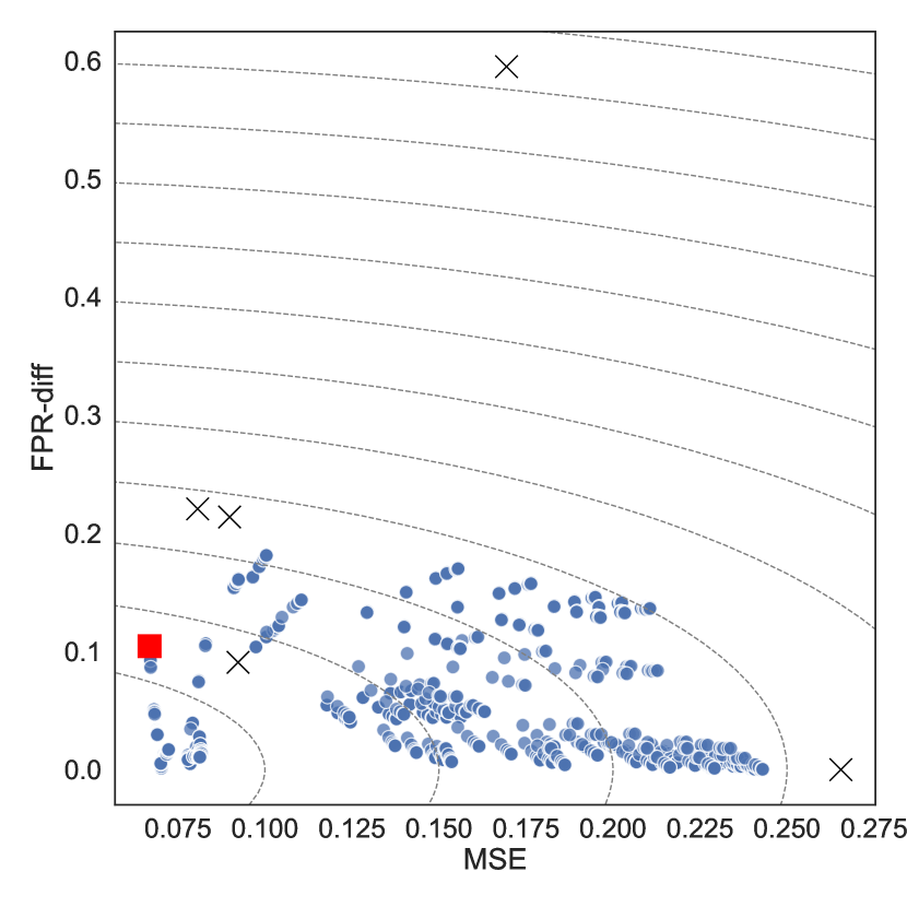
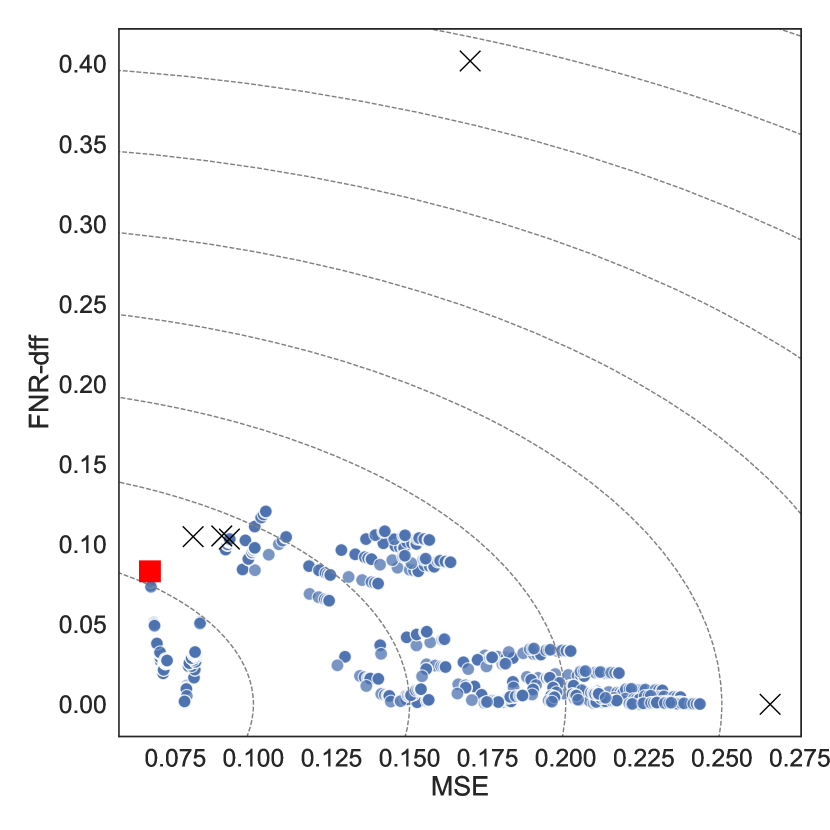
Refer to caption
Refer to caption
Refer to caption
Figure 5: Disparity and MSE values for each of 1331 predictors in the simulated data. Black “X”s represent the base predictors, with the mean predictor at the bottom right of each panel. The red square is the OLS predictor, and the blue dots are the FADE predictors. Radius lines indicate distance from the origin. Despite substantial overlap, the predictors span a wide range of fairness and accuracy values. For each disparity, many predictors exist which take that disparity to 0, at a small cost in MSE relative to the OLS predictor.
Refer to caption
Refer to caption
Refer to caption
Figure 6: Pairs of disparity values and MSE values for each of 1331 predictors in the simulated data. Black “X”s represent the base predictors, with the mean predictor at the origin in each panel. The red square is the OLS predictor, and the dots are the FADE predictors. Radius lines indicate distance from the origin. Each pair of disparities can be jointly decreased with minimal increase in MSE relative to the OLS predictor.
Predictor MSE AUC rate-diff FPR-diff FNR-diff
MSE (OLS) 0.07 0.98 0.26 0.10 0.08
MSE + rate 0.09 0.95 0.04 0.16 0.10
MSE + FPR 0.07 0.98 0.19 0.00 0.03
MSE + FNR 0.07 0.98 0.18 0.01 0.02
MSE + rate + FPR 0.12 0.90 0.04 0.05 0.09
MSE + rate + FNR 0.10 0.95 0.04 0.16 0.08
MSE + FPR + FNR 0.07 0.98 0.18 0.01 0.02
MSE + rate + FPR + FNR 0.13 0.96 0.06 0.03 0.02
Table 6: Performance of the FADE predictors that minimize the Euclidean norm of MSE and zero or more disparities, in the simulated data. The top row represents the OLS predictor, included again for reference. All three disparities can be minimized, singly or jointly, with no impact or a small impact on MSE.

7 Results: recidivism risk prediction

We next illustrate FADE on the COMPAS dataset gathered by ProPublica (Angwin and Larson, 2016; Angwin et al, 2016). The dataset comprises public arrest records, criminal records, and COMPAS scores from a single county in Florida, spanning 2013–2016. COMPAS is a collection of tools developed by the company Equivant (formerly Northpointe) designed to assess the risk of recidivism. We utilize the COMPAS scores for general, as opposed to violent, recidivism. The scores consist of risk deciles, coded 1-10, which we normalize to the range [0.1,1]0.11[0.1,1]. COMPAS takes as input up to 137 features (Northpointe, 2015; Rudin et al, 2020), which are unavailable in this dataest. We utilize just three features as covariates: an indicator for defendant age greater than 45, an indicator for defendant age less than 25, and the number of prior arrests, ranging from 0 to 29. Previous work has found that predictors trained using just these covariates perform similarly to COMPAS (Angelino et al, 2018).

The sensitive feature is race, restricted to defendants who are coded African-American (n=3175𝑛3175n=3175) or Caucasian (n=2013𝑛2013n=2013). The decision variable D𝐷D represent pretrial release, with D=0𝐷0D=0 if defendants are released and D=1𝐷1D=1 if they are detained. The outcome of interest Y0superscript𝑌0Y^{0} is rearrest within two years, should a defendant be released pretrial. Since it difficult to assess the plausibility of the positivity and ignorability assumptions without consulting with domain experts, we conducted analyses in both the counterfactual and observable setting. The results and conclusions were largely the same, so we only include the counterfactual results.

We split the data into five datasets, each with approximately 1040 rows: 𝒟learnsubscript𝒟learn\mathcal{D}_{\text{learn}}, 𝒟trainnuissuperscriptsubscript𝒟trainnuis\mathcal{D}_{\text{train}}^{\text{nuis}}, 𝒟traintargetsuperscriptsubscript𝒟traintarget\mathcal{D}_{\text{train}}^{\text{target}}, 𝒟testnuissuperscriptsubscript𝒟testnuis\mathcal{D}_{\text{test}}^{\text{nuis}}, and 𝒟testtargetsuperscriptsubscript𝒟testtarget\mathcal{D}_{\text{test}}^{\text{target}}. As base predictors, we used the four model types from the previous section as well as a logistic regression. We used random forest classifiers for the nuisance predictors in both the training and test data. Table 7 gives the estimated performance of the five base predictors, COMPAS, and the OLS predictor, which spans COMPAS and the base predictors. Previous work found differences in a binarized version of COMPAS for both observable (Angwin and Larson, 2016) and counterfactual (Mishler, 2019) false positive vs false negative rates for African-American vs. Caucasian defendants. Those differences appear here in the generalized error rates. COMPAS also has a large rate disparity. Perhaps surprisingly, the base predictors all yield smaller disparities than COMPAS, even though they generally also have smaller MSE.

We compute FADE predictors using the same sets of penalty vectors ΛΛ\Lambda as in the previous section. Figure 7 shows disparities and MSE values for all 1331 predictors. Most predictors fall within a narrow range of MSE values that also includes COMPAS, so the primary value of aggregation here is in reducing disparities. Nearly all the FADE predictors improve on COMPAS in terms of both risk and fairness. The top row of Figure 7 shows that all three disparities can be individually reduced to 0 with minimal cost in MSE relative to the OLS predictor, and the bottom row shows that these improvements also extend over pairs of disparities.

MSE rate-diff FPR-diff FNR-diff
Mean 0.26 0.00 0.00 0.00
Random Forest 0.28 0.05 0.03 0.02
Logistic 0.22 0.06 0.06 0.00
GB Classifier 0.23 0.06 0.01 0.05
Ridge 0.22 0.05 0.05 0.00
COMPAS 0.24 0.15 0.15 0.08
OLS 0.22 0.09 0.09 0.05
Table 7: Estimated performance of the five base predictors, COMPAS, and the OLS predictor in the COMPAS dataset. The OLS weights are [0.39,0.12,0.79,0.10,1.08,0.93]0.390.120.790.101.080.93[0.39,0.12,0.79,0.10,-1.08,0.93]. The OLS predictor does not perform substantially better than the base predictors. COMPAS has different false positive and false negative rates for African-American vs Caucasian defendants, as well as a rate disparity. The base predictors all have smaller disparities than COMPAS, and–perhaps surprisingly–generally smaller MSE.
Refer to caption
Refer to caption
Refer to caption
Refer to caption
Refer to caption
Refer to caption
Figure 7: Disparity against MSE (top row) or pairs of disparities colored by MSE (bottom row), for each of 1331 predictors in the COMPAS data. The black triangle represents COMPAS, the black “X”s represent the other base predictors, the red square is the OLS predictor, and the blue dots are the FADE predictors. Radius lines indicate distance from the origin. Most of the predictors improve on COMPAS in terms of both MSE and the relevant disparity. For each disparity, many predictors exist which take that disparity to 0, at a small cost in MSE relative to the OLS predictor.

8 Results: income prediction

Finally, we apply our method in the observable setting, using the Adult dataset (Dua and Graff, 2017). This dataset comprises demographic variables derived from the 1994 U.S. Census. We consider sex as a sensitive feature, coded 0 or 1, and we utilize as covariates a set of indicator variables representing age by decade, and a set of indicator variables representing the number of years of education. The classification task is to predict whether an individual’s income is over $50K/year, for example for the purpose of deciding whether to issue a loan.

We randomly split the data into four datasets: 𝒟learnsubscript𝒟learn\mathcal{D}_{\text{learn}} and 𝒟trainsubscript𝒟train\mathcal{D}_{\text{train}}, consisting of 14,653 and 14,652 rows; and 𝒟testsubscript𝒟test\mathcal{D}_{\text{test}} and 𝒟validatesubscript𝒟validate\mathcal{D}_{\text{validate}}, consisting of 9,768 and 9,769 rows. 𝒟validatesubscript𝒟validate\mathcal{D}_{\text{validate}} is used to compare the performance of the selected best predictors to predictors that are developed using existing fairness methods.

This dataset does not contain any previously trained predictors. We use the same five base predictor types as in the COMPAS analysis. Additionally, we use 𝒟trainsubscript𝒟train\mathcal{D}_{\text{train}} to train three “fair” predictors with other fairness methods: adversarial debiasing (Zhang et al, 2018), reductions (Agarwal et al, 2018), and a meta-algorithm (Celis et al, 2020). All predictors were trained using the Python library aif360, a set of tools that provide access to a range of fairness methods via a consistent interface (Bellamy et al, 2018). The three chosen methods yield binary classifiers, and they are all designed to minimize rate-diff in an observable setting with a binary outcome. Since, for a binary classifier Y^^𝑌\widehat{Y}, MSE is equal to classification error (Y^Y)^𝑌𝑌\mathbb{P}(\widehat{Y}\neq Y), we may regard these three predictors as the result of methods that seek to minimize MSE among specific classes of binary predictors.

We construct FADE predictors using the five base predictors (“base5”) or the five base predictors and the three fair predictors (“base8”). Table 8 gives the performance of the base predictors, the fair predictors, and the two OLS predictors. Compared to the base predictors, two of the three fairness methods result in a substantially lower rate-diff, which is the disparity they aim to minimize. The base predictors and the OLS predictors have lower MSE, higher AUC, and higher disparities compared to these two fair predictors.

Predictor MSE AUC rate-diff FPR-diff FNR-diff
Mean 0.18 0.50 0.00 0.00 0.00
Random Forest 0.14 0.81 0.19 0.14 0.24
Logistic 0.14 0.81 0.20 0.14 0.25
GB Classifier 0.14 0.82 0.19 0.13 0.24
Ridge 0.14 0.81 0.17 0.13 0.16
Adversarial 0.21 0.67 0.07 0.00 0.03
Reductions 0.22 0.62 0.01 0.03 0.07
Meta 0.30 0.68 0.18 0.26 0.26
OLS - base5 0.14 0.82 0.19 0.13 0.24
OLS - base8 0.14 0.81 0.20 0.14 0.25
Table 8: Estimated performance in the Adult dataset of five base predictors, three predictors trained using existing fairness methods, and the two OLS predictors, which aggregate only the five base predictors or all eight predictors. The OLS weights are [0.03,0.29,0.65,0.03,0.01]0.030.290.650.030.01[0.03,0.29,0.65,0.03,0.01], for base5, and [0.01,0.26,0.56,0.18,0.04,0.02,0.03,0]0.010.260.560.180.040.020.030[-0.01,0.26,0.56,0.18,0.04,-0.02,-0.03,0], for base8. Only two of the three fairness methods successfully control their targeted disparity, rate-diff. The Meta predictor has a rate-diff which is comparable to the base predictors which are trained without regard to fairness. The OLS predictors perform comparably to the base predictors.

We compute FADE predictors using the same sets of penalty vectors ΛΛ\Lambda as in the previous two sections. Figure 7 shows disparities and MSE values for all 1331 predictors. Fairness-accuracy tradeoffs are most evident for rate-diff and FPR-diff in the top row of this figure, where only the five base predictors are used. In the bottom row, where the fair predictors are included as basis functions, the tradeoffs essentially disappear: all three disparities can be reduced to 0 with virtually no cost in MSE.
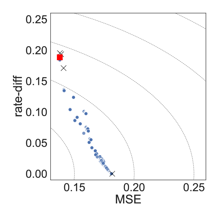
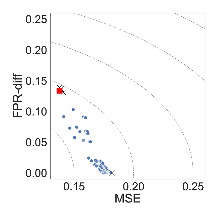
Refer to caption
Refer to caption
Refer to caption
Refer to caption
Refer to caption
Refer to caption
Figure 8: Disparity against MSE for FADE predictors based on the five base predictors (top row) or the five base predictors plus the three fair predictors, for each of 1331 FADE predictors in the Adult data. Black “X”s represent the base predictors, the red square is the OLS predictor, and the blue dots are the FADE predictors. Radius lines indicate distance from the origin. For the sake of legibility, the Meta predictor, which has an MSE of 0.30, is excluded. The top row exhibits small but clear fairness-accuracy tradeoffs for rate-diff and FPR-diff. The bottom row shows that with the inclusion of the fair predictors, each disparity can be taken to 0 with almost no cost in MSE relative to the OLS model.

8.1 Model validation

Using the performance estimates from the test data, we select the FADE predictors that minimize the distance from the origin in each of seven fairness-accuracy subspaces, for both the base5 and base8 predictors. We then compute risk and fairness estimates for each of these predictors, as well as the three fair predictors, on the validation data (Table 9). The estimates on the test and validation data differed by no more than approximately 0.005.

Both the base5 and base8 FADE predictors are substantially more fair than the OLS predictors, while incurring very small increases in MSE. The high AUC values confirm that these are accurate predictors. All the FADE predictors have small disparities compared to the OLS predictors. Explicitly minimizing multiple disparities simultaneously is not necessarily more costly in terms of performance than minimizing a single disparity.

The FADE predictors have substantially lower MSE and higher AUC than the fair predictors, and they are in many cases more fair. The fair predictors achieve values of 0.08, 0.01, and 0.17 for rate-diff, the disparity they aim to minimize. The base5 FADE predictors that include rate-diff in their criteria achieve rate-diffs of 0.04, 0.04, 0.06, and 0.02. The corresponding base8 FADE predictors achieve rate-diffs of 0.01, 0.03, 0.01, and 0.03.

The base5 results show that FADE yields predictors that perform comparably to or better than existing fairness methods. The base8 results highlight the flexibility of our approach: multiple predictors can be aggregated, regardless of whether or not they are trained with fairness properties in mind, with different weights to target different disparities. In this case, including the fair predictors in the aggregation improves both accuracy and fairness.

Each of the fair prediction methods contains tuning parameters that can be adjusted to return different predictors, as well as settings that allow them to target different fairness constraints, such as equalized odds. However, each method can only target a single fairness constraint at once. Additionally, these methods can take substantial time to run. A single run of the Meta method took roughly 5 seconds, the Reductions method ran in approximately 15 seconds, and the Adversarial method, which relies on neural nets, took roughly a minute. By contrast, we were able to train the base predictors and compute and evaluate 1331 FADE predictors in 25 seconds.

The three fair predictors are binary by construction, whereas our method returns continuous predictors. Of course, these continuous predictors can be treated as binary, either by thresholding the output (yielding a deterministic classifier) or by treating the output as a probability and sampling from a corresponding Bernoulli distribution (yielding a randomized classifier). It is fast to compute estimates of the accuracy and fairness values from either of these two binarized classifiers and choose one which minimizes the criteria of interest. For example, the base5 FADE predictors include a predictor which, when thresholded at 0.5 to yield a deterministic binary classifier, achieves a classification error of 0.24 and disparities of 0 (to two digits). This has very slightly higher classification error than the Adversarial and Reductions predictors, but it exactly achieves equalized odds and demographic parity.

Predictor MSE AUC rate-diff FPR-diff FNR-diff
base5 MSE (OLS-base5) 0.14 0.82 0.19 0.13 0.24
MSE + rate 0.16 0.73 0.04 0.02 0.10
MSE + FPR 0.15 0.80 0.09 0.06 0.13
MSE + FNR 0.16 0.75 0.10 0.09 0.01
MSE + rate + FPR 0.16 0.73 0.04 0.02 0.10
MSE + rate + FNR 0.16 0.75 0.06 0.05 0.01
MSE + FPR + FNR 0.16 0.75 0.06 0.05 0.01
MSE + rate + FPR + FNR 0.17 0.73 0.02 0.02 0.00
base8 MSE (OLS-base8) 0.14 0.81 0.20 0.14 0.25
MSE + rate 0.15 0.79 0.01 0.03 0.02
MSE + FPR 0.14 0.79 0.06 0.01 0.10
MSE + FNR 0.15 0.79 0.05 0.01 0.01
MSE + rate + FPR 0.15 0.79 0.03 0.00 0.01
MSE + rate + FNR 0.15 0.79 0.01 0.03 0.01
MSE + FPR + FNR 0.15 0.79 0.04 0.00 0.01
MSE + rate + FPR + FNR 0.15 0.79 0.03 0.01 0.01
fair Adversarial 0.21 0.67 0.08 0.01 0.04
Reductions 0.22 0.62 0.01 0.03 0.06
Meta 0.30 0.68 0.17 0.26 0.24
Table 9: Performance of the predictors that minimize the Euclidean norm of MSE and zero to three disparities, in the Adult data. The OLS predictors and the three fair predictors are included again for reference. Predictors are selected on the test data and evaluated on the validation data. The base5 FADE predictors aggregate the five base predictors, and the base8 FADE predictors aggregate all eight predictors. All three disparities can be minimized, singly or jointly, with only a small impact on MSE, and a small impact on AUC. Aggregated predictors are more accurate than the fair predictors, and have comparable or smaller values of rate-diff, the disparity that the fair predictors aim to minimize.

9 Conclusion

We developed a framework, FAir Double Ensemble learning (FADE), for constructing fair predictors and for exploring fairness-accuracy and fairness-fairness tradeoffs. This framework is extremely flexible, allowing users to combine arbitrary sets of predictors, including previously trained predictors and newly trained ones, regardless of whether they are designed to satisfy fairness constraints or not. FADE thereby collapses the distinction between in-processing and post-processing approaches to building fair predictors. FADE can accommodate a wide range of disparities and allows users to minimize multiple disparities simultaneously. FADE also accommodates both observable and counterfactual outcomes, joining a very small set of existing methods for targeting counterfactual accuracy and counterfactual versions of fairness criteria like equalized odds.

Within the FADE framework, we developed three methods. The first two “constrained” methods allow users to minimize mean squared error subject to explicit fairness constraints, or minimize unfairness subject to an explicit constraint on the mean squared error. The third “penalized” method allows users to efficiently construct large sets of predictors and evaluate their risk and fairness properties. The penalized method enables users to efficiently explore fairness-accuracy and fairness-fairness tradeoffs in their problem setting, and it enables them to find a predictor with a favorable risk and fairness profile. Our theoretical results show that FADE predictors converge to optimal behavior at fast rates, and our empirical results show that in many cases, disparities can be substantially reduced with no tangible loss of accuracy–or even an increase in accuracy–relative to the unpenalized least squares solution or an existing benchmark predictor.

Although our penalized approach is designed to minimize mean squared error and to penalize certain classes of disparities, the resulting predictors can naturally be evaluated with respect to any accuracy or fairness metric. For example, users might wish to consider only binary classifiers, so they may wish to evaluate classification error on thresholded versions of the FADE predictors. The penalized approach provides a principled way to explore various fairness-accuracy spaces, even if the fairness and/or accuracy metrics of interest aren’t explicitly represented in the penalized expression.

Finally, the efficiency of our penalized method relies on the particular closed form of the parameterized predictors, which arises as a result of the mean squared error and the squared fairness terms. However, any quadratic function that involves a positive definite matrix has a closed form solution. This form could be preserved under different accuracy metrics and fairness terms by, for example, adding a regularization term βTMβsuperscript𝛽𝑇𝑀𝛽\beta^{T}M\beta for some positive-definite matrix M𝑀M. This suggests that our approach could be adapted to explicitly target other accuracy and/or fairness metrics.

\bmhead

Acknowledgments We are grateful to Alexandra Chouldechova, Aaditya Ramdas, Cosma Shalizi, Ilya Shpitser, and Larry Wasserman for comments on earlier versions of this work. This work was completed while Alan Mishler was a PhD student at Carnegie Mellon University.

Appendix A Proof preliminaries

For convenience, we collect all the assumptions that appear in the paper, with their short descriptors:

1.  For all n𝑛n, 𝔼[bbT]𝔼delimited-[]𝑏superscript𝑏𝑇\mathbb{E}[bb^{T}] is positive definite. (PSD outer product)
2.  Uniformly in nsupw𝒲b(w)<.2.  Uniformly in nsubscriptsupremum𝑤𝒲norm𝑏𝑤\displaystyle\text{2. \-\ Uniformly in $n$, }\sup_{w\in\mathcal{W}}\|b(w)\|<\infty. (Bounded basis norm)
3.  The set {𝔼[gjb]𝔼[gjb]Tβr:j}conditional-set𝔼delimited-[]subscript𝑔𝑗𝑏𝔼superscriptdelimited-[]subscript𝑔𝑗𝑏𝑇subscriptsuperscript𝛽𝑟𝑗\{\mathbb{E}[g_{j}b]\mathbb{E}[g_{j}b]^{T}\beta^{*}_{r}:j\in\mathcal{I}\} is linearly independent. (LICQ - population)
4. Y=DY1+(1D)Y0.4. 𝑌𝐷superscript𝑌11𝐷superscript𝑌0\displaystyle\text{4. \-\ }Y=DY^{1}+(1-D)Y^{0}. (Consistency)
5. δ(0,1) s.t. (π(W)1δ)=1.5. 𝛿01 s.t. 𝜋𝑊1𝛿1\displaystyle\text{5. \-\ }\exists\delta\in(0,1)\text{ s.t. }\mathbb{P}(\pi(W)\leq 1-\delta)=1. (Positivity)
6. Y0DW.perpendicular-toabsentperpendicular-to6. superscript𝑌0conditional𝐷𝑊\displaystyle\text{6. \-\ }Y^{0}\mathchoice{\mathrel{\hbox to0.0pt{$\displaystyle\perp$\hss}\mkern 2.0mu{\displaystyle\perp}}}{\mathrel{\hbox to0.0pt{$\textstyle\perp$\hss}\mkern 2.0mu{\textstyle\perp}}}{\mathrel{\hbox to0.0pt{$\scriptstyle\perp$\hss}\mkern 2.0mu{\scriptstyle\perp}}}{\mathrel{\hbox to0.0pt{$\scriptscriptstyle\perp$\hss}\mkern 2.0mu{\scriptscriptstyle\perp}}}D\mid W. (Ignorability)
7. γ(0,1) s.t. (π^(A,X,S)1γ)=1.7. 𝛾01 s.t. ^𝜋𝐴𝑋𝑆1𝛾1\displaystyle\text{7. \-\ }\exists\gamma\in(0,1)\text{ s.t. }\mathbb{P}(\widehat{\pi}(A,X,S)\leq 1-\gamma)=1. (Bounded propensity estimator)
8. π^π=o(1) and μ^0μ0=o(1) and ν^0ν0=o(1).8. norm^𝜋𝜋subscript𝑜1 and normsubscript^𝜇0subscript𝜇0subscript𝑜1 and normsubscript^𝜈0subscript𝜈0subscript𝑜1\displaystyle\text{8. \-\ }\|\widehat{\pi}-\pi\|=o_{\mathbb{P}}(1)\text{ and }\|\widehat{\mu}_{0}-\mu_{0}\|=o_{\mathbb{P}}(1)\text{ and }\|\widehat{\nu}_{0}-\nu_{0}\|=o_{\mathbb{P}}(1). (Consistent nuisance estimators)
9. π^πμ^0μ0=o(1/n).9. norm^𝜋𝜋normsubscript^𝜇0subscript𝜇0subscript𝑜1𝑛\displaystyle\text{9. \-\ }\|\widehat{\pi}-\pi\|\|\widehat{\mu}_{0}-\mu_{0}\|=o_{\mathbb{P}}(1/\sqrt{n}). (Nuisance parameter rates)
π^πν^0ν0=o(1/n).norm^𝜋𝜋normsubscript^𝜈0subscript𝜈0subscript𝑜1𝑛\displaystyle\quad\-\ \|\widehat{\pi}-\pi\|\|\widehat{\nu}_{0}-\nu_{0}\|=o_{\mathbb{P}}(1/\sqrt{n}).
10. ΛnΛt for some compact Λ.10. subscriptΛ𝑛Λsuperscript𝑡 for some compact Λ\displaystyle\text{10. \-\ }\Lambda_{n}\subseteq\Lambda\subset\mathbb{R}^{t}\text{ for some compact }\Lambda. (Compact ΛΛ\Lambda)

Recall that for any function f:𝒵:𝑓maps-to𝒵f:\mathcal{Z}\mapsto\mathbb{R}, we defined n(f)=n1j=1nf=f𝑑n(Z)subscript𝑛𝑓superscript𝑛1superscriptsubscript𝑗1𝑛𝑓𝑓differential-dsubscript𝑛𝑍\mathbb{P}_{n}(f)=n^{-1}\sum_{j=1}^{n}f=\int fd\mathbb{P}_{n}(Z) and (f)=f𝑑(Z)𝑓𝑓differential-d𝑍\mathbb{P}(f)=\int fd\mathbb{P}(Z) as the sample and population expectations of f𝑓f, so that for example (ϕ^)=𝔼[ϕ^𝒟train]^italic-ϕ𝔼delimited-[]conditional^italic-ϕsubscript𝒟train\mathbb{P}(\widehat{\phi})=\mathbb{E}[\widehat{\phi}\mid\mathcal{D}_{\text{train}}] or 𝔼[ϕ^𝒟test]𝔼delimited-[]conditional^italic-ϕsubscript𝒟test\mathbb{E}[\widehat{\phi}\mid\mathcal{D}_{\text{test}}] is the expected value of ϕ^(Z)^italic-ϕ𝑍\widehat{\phi}(Z) once the relevant nuisance function estimate ϕ^^italic-ϕ\widehat{\phi} has been constructed.

We state several lemmas that are used in the proofs for the constrained and penalized settings. The first is a restatement of Lemma 2 in Kennedy et al (2020).

Lemma 1 (Kennedy, 2020).

Let f^:𝒵:^𝑓maps-to𝒵\widehat{f}:\mathcal{Z}\mapsto\mathbb{R} be a function estimated on a nuisance dataset 𝒟nuissuperscript𝒟nuis\mathcal{D}^{\text{nuis}} independent of nsubscript𝑛\mathbb{P}_{n}, and let f:𝒵:𝑓maps-to𝒵f:\mathcal{Z}\mapsto\mathbb{R} be another function. Assume var(f^f𝒟nuis)<var^𝑓conditional𝑓superscript𝒟nuis\ \mbox{\rm\bf\sf var}\ (\widehat{f}-f\mid\mathcal{D}^{\text{nuis}})<\infty. Then

(n)(f^f)subscript𝑛^𝑓𝑓\displaystyle(\mathbb{P}_{n}-\mathbb{P})(\widehat{f}-f) =O(f^fn)absentsubscript𝑂norm^𝑓𝑓𝑛\displaystyle=O_{\mathbb{P}}\left(\frac{\|\widehat{f}-f\|}{\sqrt{n}}\right)
Lemma 2 (Double robustness).

Let f:𝒲p:𝑓maps-to𝒲superscript𝑝f:\mathcal{W}\mapsto\mathbb{R}^{p} for any p𝑝p be a function with f(W)M<norm𝑓𝑊𝑀\|f(W)\|\leq M<\infty for some M𝑀M. Under Assumption 5 (positivity),

f(W)(ϕ^ϕ)norm𝑓𝑊^italic-ϕitalic-ϕ\displaystyle\|f(W)(\widehat{\phi}-\phi)\| =O(μ0μ^0π^π)absentsubscript𝑂normsubscript𝜇0subscript^𝜇0norm^𝜋𝜋\displaystyle=O_{\mathbb{P}}\left(\|\mu_{0}-\widehat{\mu}_{0}\|\|\widehat{\pi}-\pi\|\right)
f(W)(ϕ¯^ϕ¯)norm𝑓𝑊^¯italic-ϕ¯italic-ϕ\displaystyle\|f(W)(\widehat{\underline{\phi}}-\underline{\phi})\| =O(ν0ν^0π^π)absentsubscript𝑂normsubscript𝜈0subscript^𝜈0norm^𝜋𝜋\displaystyle=O_{\mathbb{P}}\left(\|\nu_{0}-\widehat{\nu}_{0}\|\|\widehat{\pi}-\pi\|\right)

It follows immediately that

(f(W)(ϕ^ϕ))𝑓𝑊^italic-ϕitalic-ϕ\displaystyle\mathbb{P}\left(f(W)(\widehat{\phi}-\phi)\right) =O(μ0μ^0π^π)absentsubscript𝑂normsubscript𝜇0subscript^𝜇0norm^𝜋𝜋\displaystyle=O_{\mathbb{P}}\left(\|\mu_{0}-\widehat{\mu}_{0}\|\|\widehat{\pi}-\pi\|\right)
(f(W)(ϕ¯^ϕ¯))𝑓𝑊^¯italic-ϕ¯italic-ϕ\displaystyle\mathbb{P}\left(f(W)(\widehat{\underline{\phi}}-\underline{\phi})\right) =O(ν0ν^0π^π)absentsubscript𝑂normsubscript𝜈0subscript^𝜈0norm^𝜋𝜋\displaystyle=O_{\mathbb{P}}\left(\|\nu_{0}-\widehat{\nu}_{0}\|\|\widehat{\pi}-\pi\|\right)

Proof:

(f(W)(ϕ^ϕ))𝑓𝑊^italic-ϕitalic-ϕ\displaystyle\mathbb{P}\left(f(W)(\widehat{\phi}-\phi)\right) =(f(W)(1D1π^(Yμ^0)+μ^01D1π(Yμ0)μ0))absent𝑓𝑊1𝐷1^𝜋𝑌subscript^𝜇0subscript^𝜇01𝐷1𝜋𝑌subscript𝜇0subscript𝜇0\displaystyle=\mathbb{P}\left(f(W)\left(\frac{1-D}{1-\widehat{\pi}}(Y-\widehat{\mu}_{0})+\widehat{\mu}_{0}-\frac{1-D}{1-\pi}(Y-\mu_{0})-\mu_{0}\right)\right)
=(f(W)(1D1π^(μ0μ^0)+μ^01D1π(μ0μ0)μ0))absent𝑓𝑊1𝐷1^𝜋subscript𝜇0subscript^𝜇0subscript^𝜇01𝐷1𝜋subscript𝜇0subscript𝜇0subscript𝜇0\displaystyle=\mathbb{P}\left(f(W)\left(\frac{1-D}{1-\widehat{\pi}}(\mu_{0}-\widehat{\mu}_{0})+\widehat{\mu}_{0}-\frac{1-D}{1-\pi}(\mu_{0}-\mu_{0})-\mu_{0}\right)\right)
=(f(W)(1π1π^(μ0μ^0)+μ^0μ0))absent𝑓𝑊1𝜋1^𝜋subscript𝜇0subscript^𝜇0subscript^𝜇0subscript𝜇0\displaystyle=\mathbb{P}\left(f(W)\left(\frac{1-\pi}{1-\widehat{\pi}}(\mu_{0}-\widehat{\mu}_{0})+\widehat{\mu}_{0}-\mu_{0}\right)\right)
=(f(W)((μ0μ^0)(π^π)1π))absent𝑓𝑊subscript𝜇0subscript^𝜇0^𝜋𝜋1𝜋\displaystyle=\mathbb{P}\left(f(W)\left(\frac{(\mu_{0}-\widehat{\mu}_{0})(\widehat{\pi}-\pi)}{1-\pi}\right)\right)
1δ(f(W)(μ0μ^0)(π^π))absent1𝛿𝑓𝑊subscript𝜇0subscript^𝜇0^𝜋𝜋\displaystyle\leq\frac{1}{\delta}\mathbb{P}(f(W)(\mu_{0}-\widehat{\mu}_{0})(\widehat{\pi}-\pi))
1δf(W)μ0μ^0π^πabsent1𝛿norm𝑓𝑊normsubscript𝜇0subscript^𝜇0norm^𝜋𝜋\displaystyle\leq\frac{1}{\delta}\|f(W)\|\|\mu_{0}-\widehat{\mu}_{0}\|\|\widehat{\pi}-\pi\|
=O(μ0μ^0π^π)absentsubscript𝑂normsubscript𝜇0subscript^𝜇0norm^𝜋𝜋\displaystyle=O_{\mathbb{P}}\left(\|\mu_{0}-\widehat{\mu}_{0}\|\|\widehat{\pi}-\pi\|\right)

where the second and third lines use iterated expectation, conditioning on W𝑊W; the fifth line uses Assumption 5 (positivity); and the sixth line uses the Cauchy-Schwarz inequality.

Appendix B Proofs of propositions

B.1 Proof of Proposition 1

Proof: Let α0,α1subscript𝛼0subscript𝛼1\alpha_{0},\alpha_{1}\in\mathbb{R}, let h0,h1subscript0subscript1h_{0},h_{1} be mappings from {0,1}×Y~01~𝑌\{0,1\}\times\widetilde{Y} to {0,1}01\{0,1\}, and let g(W,Y~)=α0h0(A,Y~)𝔼[h0(A,Y~)]α1h1(A,Y~)𝔼[h1(A,Y~)]𝑔𝑊~𝑌subscript𝛼0subscript0𝐴~𝑌𝔼delimited-[]subscript0𝐴~𝑌subscript𝛼1subscript1𝐴~𝑌𝔼delimited-[]subscript1𝐴~𝑌g(W,\widetilde{Y})=\alpha_{0}\frac{h_{0}(A,\widetilde{Y})}{\mathbb{E}[h_{0}(A,\widetilde{Y})]}-\alpha_{1}\frac{h_{1}(A,\widetilde{Y})}{\mathbb{E}[h_{1}(A,\widetilde{Y})]}. Then

𝔼[f(W)h0(A,Y~)]𝔼delimited-[]𝑓𝑊subscript0𝐴~𝑌\displaystyle\mathbb{E}[f(W)h_{0}(A,\widetilde{Y})] =𝔼[𝔼[f(W)h0(A,Y~)h0(A,Y~)]]absent𝔼delimited-[]𝔼delimited-[]conditional𝑓𝑊subscript0𝐴~𝑌subscript0𝐴~𝑌\displaystyle=\mathbb{E}[\mathbb{E}[f(W)h_{0}(A,\widetilde{Y})\mid h_{0}(A,\widetilde{Y})]]
=𝔼[f(W)h0(A,Y~)=1](h0(A,Y~)=1)absent𝔼delimited-[]conditional𝑓𝑊subscript0𝐴~𝑌1subscript0𝐴~𝑌1\displaystyle=\mathbb{E}[f(W)\mid h_{0}(A,\widetilde{Y})=1]\mathbb{P}(h_{0}(A,\widetilde{Y})=1)
=𝔼[f(W)h0(A,Y~)=1]𝔼[h0(A,Y~)]absent𝔼delimited-[]conditional𝑓𝑊subscript0𝐴~𝑌1𝔼delimited-[]subscript0𝐴~𝑌\displaystyle=\mathbb{E}[f(W)\mid h_{0}(A,\widetilde{Y})=1]\mathbb{E}[h_{0}(A,\widetilde{Y})]
𝔼[f(W)h0(A,Y~)=1]absent𝔼delimited-[]conditional𝑓𝑊subscript0𝐴~𝑌1\displaystyle\implies\mathbb{E}[f(W)\mid h_{0}(A,\widetilde{Y})=1] =𝔼[f(W)h0(A,Y~)]𝔼[h0(A,Y~)]absent𝔼delimited-[]𝑓𝑊subscript0𝐴~𝑌𝔼delimited-[]subscript0𝐴~𝑌\displaystyle=\frac{\mathbb{E}[f(W)h_{0}(A,\widetilde{Y})]}{\mathbb{E}[h_{0}(A,\widetilde{Y})]}

where 𝔼[h0(A,Y~)]>0𝔼delimited-[]subscript0𝐴~𝑌0\mathbb{E}[h_{0}(A,\widetilde{Y})]>0 by assumption. By similar reasoning for h1subscript1h_{1}, it follows that

|α0𝔼[f(W)h0(A,Y~)=1]α1𝔼[f(W)h1(A,Y~)=1]|subscript𝛼0𝔼delimited-[]conditional𝑓𝑊subscript0𝐴~𝑌1subscript𝛼1𝔼delimited-[]conditional𝑓𝑊subscript1𝐴~𝑌1\displaystyle\lvert\alpha_{0}\mathbb{E}[f(W)\mid h_{0}(A,\widetilde{Y})=1]-\alpha_{1}\mathbb{E}[f(W)\mid h_{1}(A,\widetilde{Y})=1]\rvert =|𝔼[g(W,Y~)f(W)]|absent𝔼delimited-[]𝑔𝑊~𝑌𝑓𝑊\displaystyle=\lvert\mathbb{E}[g(W,\widetilde{Y})f(W)]\rvert

as desired.

B.2 Proof of Proposition 2

Proof: Define the Lagrangian L(β,v)𝐿𝛽𝑣L(\beta,v) of the risk-min program that defines βrsubscriptsuperscript𝛽𝑟\beta^{*}_{r}:

L(β,v)𝐿𝛽𝑣\displaystyle L(\beta,v) =𝔼[(bTβY~)2]+j=1tvj{(𝔼[gjbTβ])2ϵj2}absent𝔼delimited-[]superscriptsuperscript𝑏𝑇𝛽~𝑌2superscriptsubscript𝑗1𝑡subscript𝑣𝑗superscript𝔼delimited-[]subscript𝑔𝑗superscript𝑏𝑇𝛽2superscriptsubscriptitalic-ϵ𝑗2\displaystyle=\mathbb{E}[(b^{T}\beta-\widetilde{Y})^{2}]+\sum_{j=1}^{t}v_{j}\left\{\left(\mathbb{E}[g_{j}b^{T}\beta]\right)^{2}-\epsilon_{j}^{2}\right\}

Under Assumption 1, the risk-min program is a strictly convex quadratic program, and it is feasible by construction. Therefore, the dual program has at least one solution λ0+t𝜆superscriptsubscriptlimit-from0𝑡\lambda\in\mathbb{R}_{0+}^{t}, and strong duality holds, so the primal solution βrsubscriptsuperscript𝛽𝑟\beta^{*}_{r} and λ𝜆\lambda jointly satisfy the KKT conditions. In particular, βL(βr,λ)=0subscript𝛽𝐿subscriptsuperscript𝛽𝑟𝜆0\nabla_{\beta}L(\beta^{*}_{r},\lambda)=0 (stationarity). By computing βL(β,u)subscript𝛽𝐿𝛽𝑢\nabla_{\beta}L(\beta,u), we see that this equality holds iff

βrsubscriptsuperscript𝛽𝑟\displaystyle\beta^{*}_{r} =(𝔼[bbT]+j=1tλj𝔼[gjb]𝔼[gjb]T)1𝔼[Y~b]absentsuperscript𝔼delimited-[]𝑏superscript𝑏𝑇superscriptsubscript𝑗1𝑡subscript𝜆𝑗𝔼delimited-[]subscript𝑔𝑗𝑏𝔼superscriptdelimited-[]subscript𝑔𝑗𝑏𝑇1𝔼delimited-[]~𝑌𝑏\displaystyle=\left(\mathbb{E}[bb^{T}]+\sum_{j=1}^{t}\lambda_{j}\mathbb{E}[g_{j}b]\mathbb{E}[g_{j}b]^{T}\right)^{-1}\mathbb{E}[\widetilde{Y}b]
=βλabsentsubscriptsuperscript𝛽𝜆\displaystyle=\beta^{*}_{\lambda}

If Assumption 3 holds, then λ𝜆\lambda is unique by Theorem 2 in Wachsmuth (2013).

B.3 Proof of Proposition 3

Proof: Assumption 1 again ensures that βλsubscriptsuperscript𝛽𝜆\beta^{*}_{\lambda} exists and is unique. The KKT conditions for the risk-min program are satisfied by setting ϵj2=(n[g^jbTβ^λ])2superscriptsubscriptitalic-ϵ𝑗2superscriptsubscript𝑛delimited-[]subscript^𝑔𝑗superscript𝑏𝑇subscript^𝛽𝜆2\epsilon_{j}^{2}=(\mathbb{P}_{n}[\widehat{g}_{j}b^{T}{\widehat{\beta}}_{\lambda}])^{2}, which then implies that

βλ=subscriptsuperscript𝛽𝜆absent\displaystyle\beta^{*}_{\lambda}= argminβk𝔼[(bTβY~)2]subscriptargmin𝛽superscript𝑘𝔼delimited-[]superscriptsuperscript𝑏𝑇𝛽~𝑌2\displaystyle\operatorname*{arg\,min}_{\beta\in\mathbb{R}^{k}}\mathbb{E}[(b^{T}\beta-\widetilde{Y})^{2}]
subject to (𝔼[gjbTβ])2(n[g^jbTβ^λ])2,j=1,tformulae-sequencesubject to superscript𝔼delimited-[]subscript𝑔𝑗superscript𝑏𝑇𝛽2superscriptsubscript𝑛delimited-[]subscript^𝑔𝑗superscript𝑏𝑇subscript^𝛽𝜆2𝑗1𝑡\displaystyle\text{subject to }\-\ (\mathbb{E}[g_{j}b^{T}\beta])^{2}\leq(\mathbb{P}_{n}[\widehat{g}_{j}b^{T}{\widehat{\beta}}_{\lambda}])^{2},\quad j=1,\ldots t
=\displaystyle= βrsubscriptsuperscript𝛽𝑟\displaystyle\beta^{*}_{r}

B.4 Proof of Proposition 4

Proof: Beginning with the risk, note that

var(Y0)varsuperscript𝑌0\displaystyle\ \mbox{\rm\bf\sf var}\ (Y^{0}) =𝔼[(Y0)2](𝔼[Y0])2absent𝔼delimited-[]superscriptsuperscript𝑌02superscript𝔼delimited-[]superscript𝑌02\displaystyle=\mathbb{E}[(Y^{0})^{2}]-(\mathbb{E}[Y^{0}])^{2}
=𝔼{𝔼[(Y0)2W]}(𝔼{𝔼[Y0W]})2absent𝔼𝔼delimited-[]conditionalsuperscriptsuperscript𝑌02𝑊superscript𝔼𝔼delimited-[]conditionalsuperscript𝑌0𝑊2\displaystyle=\mathbb{E}\{\mathbb{E}[(Y^{0})^{2}\mid W]\}-(\mathbb{E}\{\mathbb{E}[Y^{0}\mid W]\})^{2}
=𝔼{𝔼[Y2W,D=0]}(𝔼{𝔼[YW,D=0]})2absent𝔼𝔼delimited-[]conditionalsuperscript𝑌2𝑊𝐷0superscript𝔼𝔼delimited-[]conditional𝑌𝑊𝐷02\displaystyle=\mathbb{E}\{\mathbb{E}[Y^{2}\mid W,D=0]\}-(\mathbb{E}\{\mathbb{E}[Y\mid W,D=0]\})^{2}
=𝔼[ν0](𝔼[μ0])2absent𝔼delimited-[]subscript𝜈0superscript𝔼delimited-[]subscript𝜇02\displaystyle=\mathbb{E}[\nu_{0}]-(\mathbb{E}[\mu_{0}])^{2}

where the second line uses iterated expectation and the third line follows from the consistency and ignorability assumptions. We then have

𝔼[(fY0)2]𝔼delimited-[]superscript𝑓superscript𝑌02\displaystyle\mathbb{E}[(f-Y^{0})^{2}] =𝔼{𝔼[f22Y0+(Y0)2W]}absent𝔼𝔼delimited-[]superscript𝑓22superscript𝑌0conditionalsuperscriptsuperscript𝑌02𝑊\displaystyle=\mathbb{E}\{\mathbb{E}[f^{2}-2Y^{0}+(Y^{0})^{2}\mid W]\}
=𝔼[f22μ0+ν0]absent𝔼delimited-[]superscript𝑓22subscript𝜇0subscript𝜈0\displaystyle=\mathbb{E}[f^{2}-2\mu_{0}+\nu_{0}]
=𝔼[(fμ0)2]+(𝔼[ν0]𝔼[μ02])]]\displaystyle=\mathbb{E}[(f-\mu_{0})^{2}]+(\mathbb{E}[\nu_{0}]-\mathbb{E}[\mu_{0}^{2}])]]
=𝔼[(fμ0)2]+var(Y0)absent𝔼delimited-[]superscript𝑓subscript𝜇02varsuperscript𝑌0\displaystyle=\mathbb{E}[(f-\mu_{0})^{2}]+\ \mbox{\rm\bf\sf var}\ (Y^{0})

The last and third-to-last lines give the equalities in the proposition. Turning to the FPR-diff, by Definition 2 and Proposition 1, we have

𝔼[gcFPRf(W)]𝔼delimited-[]superscript𝑔cFPR𝑓𝑊\displaystyle\mathbb{E}[g^{\text{cFPR}}f(W)] =𝔼[{(1Y0)(1A)𝔼[(1Y0)(1A)](1Y0)A𝔼[(1Y0)A]}f(W)]absent𝔼delimited-[]1superscript𝑌01𝐴𝔼delimited-[]1superscript𝑌01𝐴1superscript𝑌0𝐴𝔼delimited-[]1superscript𝑌0𝐴𝑓𝑊\displaystyle=\mathbb{E}\left[\left\{\frac{(1-Y^{0})(1-A)}{\mathbb{E}[(1-Y^{0})(1-A)]}-\frac{(1-Y^{0})A}{\mathbb{E}[(1-Y^{0})A]}\right\}f(W)\right]
=𝔼[𝔼{(1Y0)(1A)𝔼[(1Y0)(1A)](1Y0)A𝔼[(1Y0)A]|W}f(W)]absent𝔼delimited-[]𝔼conditional-set1superscript𝑌01𝐴𝔼delimited-[]1superscript𝑌01𝐴1superscript𝑌0𝐴𝔼delimited-[]1superscript𝑌0𝐴𝑊𝑓𝑊\displaystyle=\mathbb{E}\left[\mathbb{E}\left\{\frac{(1-Y^{0})(1-A)}{\mathbb{E}[(1-Y^{0})(1-A)]}-\frac{(1-Y^{0})A}{\mathbb{E}[(1-Y^{0})A]}\-\ \Big{|}\-\ W\right\}f(W)\right]
=𝔼[{(1μ0)(1A)𝔼[(1μ0)(1A)](1μ0)A𝔼[(1μ0)A]}f(W)]absent𝔼delimited-[]1subscript𝜇01𝐴𝔼delimited-[]1subscript𝜇01𝐴1subscript𝜇0𝐴𝔼delimited-[]1subscript𝜇0𝐴𝑓𝑊\displaystyle=\mathbb{E}\left[\left\{\frac{(1-\mu_{0})(1-A)}{\mathbb{E}[(1-\mu_{0})(1-A)]}-\frac{(1-\mu_{0})A}{\mathbb{E}[(1-\mu_{0})A]}\right\}f(W)\right]

where the last line again follows from the consistency and ignorability assumptions. The result for gcFNRsuperscript𝑔cFNRg^{\text{cFNR}} follows by identical reasoning.

Appendix C Proof of Theorem 5

We prove this theorem first, since the result is used in the proofs of the other theorems. In the observable setting, the theorem follows immediately from the central limit theorem, so the subsequent derivations are for the counterfactual setting.

C.1 Asymptotic normality of the risk estimator

For any fixed predictor fβsubscript𝑓𝛽f_{\beta}, we have

Risk^(fβ)Risk(fβ)=^Risksubscript𝑓𝛽Risksubscript𝑓𝛽absent\displaystyle\widehat{\operatorname{Risk}}(f_{\beta})-\operatorname{Risk}(f_{\beta})= n[fβ2(2bTβ)ϕ^+ϕ¯^][fβ2(2bTβ)ϕ+ϕ¯]subscript𝑛delimited-[]superscriptsubscript𝑓𝛽22superscript𝑏𝑇𝛽^italic-ϕ^¯italic-ϕdelimited-[]superscriptsubscript𝑓𝛽22superscript𝑏𝑇𝛽italic-ϕ¯italic-ϕ\displaystyle\-\ \mathbb{P}_{n}[f_{\beta}^{2}-(2b^{T}\beta)\widehat{\phi}+\widehat{\underline{\phi}}]-\mathbb{P}[f_{\beta}^{2}-(2b^{T}\beta)\phi+\underline{\phi}]
=\displaystyle= (n){fβ22fβϕ+ϕ¯}+limit-fromsubscript𝑛superscriptsubscript𝑓𝛽22subscript𝑓𝛽italic-ϕ¯italic-ϕ\displaystyle\-\ (\mathbb{P}_{n}-\mathbb{P})\left\{f_{\beta}^{2}-2f_{\beta}\phi+\underline{\phi}\right\}+
(n){2fβ(ϕϕ^)+(ϕ¯^ϕ¯)}+limit-fromsubscript𝑛2subscript𝑓𝛽italic-ϕ^italic-ϕ^¯italic-ϕ¯italic-ϕ\displaystyle\-\ (\mathbb{P}_{n}-\mathbb{P})\left\{2f_{\beta}(\phi-\widehat{\phi})+(\widehat{\underline{\phi}}-\underline{\phi})\right\}+
{2fβ(ϕϕ^)+(ϕ¯^ϕ¯)}2subscript𝑓𝛽italic-ϕ^italic-ϕ^¯italic-ϕ¯italic-ϕ\displaystyle\-\ \mathbb{P}\left\{2f_{\beta}(\phi-\widehat{\phi})+(\widehat{\underline{\phi}}-\underline{\phi})\right\}

The second term of the last equality is O(μ^0μ0π^π/n)=o(1/n)subscript𝑂normsubscript^𝜇0subscript𝜇0norm^𝜋𝜋𝑛subscript𝑜1𝑛O_{\mathbb{P}}(\|\widehat{\mu}_{0}-\mu_{0}\|\|\widehat{\pi}-\pi\|/\sqrt{n})=o_{\mathbb{P}}(1/\sqrt{n}) by Lemma 1, Lemma 2, and Assumption 9. The third term is o(1/n)subscript𝑜1𝑛o_{\mathbb{P}}(1/\sqrt{n}) by Lemma 2 and Assumption 9. We therefore have

Risk^(fβ)Risk(fβ)^Risksubscript𝑓𝛽Risksubscript𝑓𝛽\displaystyle\widehat{\operatorname{Risk}}(f_{\beta})-\operatorname{Risk}(f_{\beta}) =(n){fβ22fβϕ+ϕ¯}+o(1/n)absentsubscript𝑛superscriptsubscript𝑓𝛽22subscript𝑓𝛽italic-ϕ¯italic-ϕsubscript𝑜1𝑛\displaystyle=(\mathbb{P}_{n}-\mathbb{P})\left\{f_{\beta}^{2}-2f_{\beta}\phi+\underline{\phi}\right\}+o_{\mathbb{P}}(1/\sqrt{n}) (4)

and the result follows by the central limit theorem.

C.2 Asymptotic normality of the unfairness estimators

Since gratesuperscript𝑔rateg^{\text{rate}} does not depend on the outcome, we have g^ind=gratesuperscript^𝑔indsuperscript𝑔rate\widehat{g}^{\text{ind}}=g^{\text{rate}}, and the result follows immediately from the central limit theorem. We now prove the result for gFPRsuperscript𝑔FPRg^{\text{FPR}} in the counterfactual setting. We have

n(g^jfβ)(gjfβ)subscript𝑛subscript^𝑔𝑗subscript𝑓𝛽subscript𝑔𝑗subscript𝑓𝛽\displaystyle\mathbb{P}_{n}(\widehat{g}_{j}f_{\beta})-\mathbb{P}(g_{j}f_{\beta}) ={n[γ^0fβ]n[γ^0]n[γ^1fβ]n[γ^1]}{[γ0fβ][γ0][γ1fβ][γ1]}absentsubscript𝑛delimited-[]subscript^𝛾0subscript𝑓𝛽subscript𝑛delimited-[]subscript^𝛾0subscript𝑛delimited-[]subscript^𝛾1subscript𝑓𝛽subscript𝑛delimited-[]subscript^𝛾1delimited-[]subscript𝛾0subscript𝑓𝛽delimited-[]subscript𝛾0delimited-[]subscript𝛾1subscript𝑓𝛽delimited-[]subscript𝛾1\displaystyle=\left\{\frac{\mathbb{P}_{n}[\widehat{\gamma}_{0}f_{\beta}]}{\mathbb{P}_{n}[\widehat{\gamma}_{0}]}-\frac{\mathbb{P}_{n}[\widehat{\gamma}_{1}f_{\beta}]}{\mathbb{P}_{n}[\widehat{\gamma}_{1}]}\right\}-\left\{\frac{\mathbb{P}[\gamma_{0}f_{\beta}]}{\mathbb{P}[\gamma_{0}]}-\frac{\mathbb{P}[\gamma_{1}f_{\beta}]}{\mathbb{P}[\gamma_{1}]}\right\} (5)

Considering just the γ^0subscript^𝛾0\widehat{\gamma}_{0} and γ0subscript𝛾0\gamma_{0} terms, we have

n[γ^0fβ]n[γ^0][γ0fβ][γ0]=n[γ^0fβ][γ0][γ0]n[γ^0]n[γ^0][γ0]subscript𝑛delimited-[]subscript^𝛾0subscript𝑓𝛽subscript𝑛delimited-[]subscript^𝛾0delimited-[]subscript𝛾0subscript𝑓𝛽delimited-[]subscript𝛾0subscript𝑛delimited-[]subscript^𝛾0subscript𝑓𝛽delimited-[]subscript𝛾0delimited-[]subscript𝛾0subscript𝑛delimited-[]subscript^𝛾0subscript𝑛delimited-[]subscript^𝛾0delimited-[]subscript𝛾0\displaystyle\frac{\mathbb{P}_{n}[\widehat{\gamma}_{0}f_{\beta}]}{\mathbb{P}_{n}[\widehat{\gamma}_{0}]}-\frac{\mathbb{P}[\gamma_{0}f_{\beta}]}{\mathbb{P}[\gamma_{0}]}=\frac{\mathbb{P}_{n}[\widehat{\gamma}_{0}f_{\beta}]\mathbb{P}[\gamma_{0}]-\mathbb{P}[\gamma_{0}]\mathbb{P}_{n}[\widehat{\gamma}_{0}]}{\mathbb{P}_{n}[\widehat{\gamma}_{0}]\mathbb{P}[\gamma_{0}]}
=[γ0](n[γ^0fβ][γ0fβ])[γ0fβ](n[γ^0][γ0])n[γ^0][γ0]absentdelimited-[]subscript𝛾0subscript𝑛delimited-[]subscript^𝛾0subscript𝑓𝛽delimited-[]subscript𝛾0subscript𝑓𝛽delimited-[]subscript𝛾0subscript𝑓𝛽subscript𝑛delimited-[]subscript^𝛾0delimited-[]subscript𝛾0subscript𝑛delimited-[]subscript^𝛾0delimited-[]subscript𝛾0\displaystyle=\frac{\mathbb{P}[\gamma_{0}]\Big{(}\mathbb{P}_{n}[\widehat{\gamma}_{0}f_{\beta}]-\mathbb{P}[\gamma_{0}f_{\beta}]\Big{)}-\mathbb{P}[\gamma_{0}f_{\beta}]\Big{(}\mathbb{P}_{n}[\widehat{\gamma}_{0}]-\mathbb{P}[\gamma_{0}]\Big{)}}{\mathbb{P}_{n}[\widehat{\gamma}_{0}]\mathbb{P}[\gamma_{0}]}
=n[γ^0]1{(n[γ^0fβ][γ0fβ])(1)[γ0fβ][γ0](n[γ^0][γ0])(2)}absentsubscript𝑛superscriptdelimited-[]subscript^𝛾01subscriptsubscript𝑛delimited-[]subscript^𝛾0subscript𝑓𝛽delimited-[]subscript𝛾0subscript𝑓𝛽1delimited-[]subscript𝛾0subscript𝑓𝛽delimited-[]subscript𝛾0subscriptsubscript𝑛delimited-[]subscript^𝛾0delimited-[]subscript𝛾02\displaystyle=\mathbb{P}_{n}[\widehat{\gamma}_{0}]^{-1}\Big{\{}\underbrace{\left(\mathbb{P}_{n}[\widehat{\gamma}_{0}f_{\beta}]-\mathbb{P}[\gamma_{0}f_{\beta}]\right)}_{(1)}-\frac{\mathbb{P}[\gamma_{0}f_{\beta}]}{\mathbb{P}[\gamma_{0}]}\underbrace{(\mathbb{P}_{n}[\widehat{\gamma}_{0}]-\mathbb{P}[\gamma_{0}])}_{(2)}\Big{\}} (6)

Terms (1) and (2) in (6) can be expanded as follows:

(1)1\displaystyle(1) =(n)γ0fβ+(n)((γ^0γ0)fβ)+((γ^0γ0)fβ)absentsubscript𝑛subscript𝛾0subscript𝑓𝛽subscript𝑛subscript^𝛾0subscript𝛾0subscript𝑓𝛽subscript^𝛾0subscript𝛾0subscript𝑓𝛽\displaystyle=(\mathbb{P}_{n}-\mathbb{P})\gamma_{0}f_{\beta}+(\mathbb{P}_{n}-\mathbb{P})((\widehat{\gamma}_{0}-\gamma_{0})f_{\beta})+\mathbb{P}((\widehat{\gamma}_{0}-\gamma_{0})f_{\beta})
(2)2\displaystyle(2) =(n)γ0+(n)(γ^0γ0)+(γ^0γ0)absentsubscript𝑛subscript𝛾0subscript𝑛subscript^𝛾0subscript𝛾0subscript^𝛾0subscript𝛾0\displaystyle=(\mathbb{P}_{n}-\mathbb{P})\gamma_{0}+(\mathbb{P}_{n}-\mathbb{P})(\widehat{\gamma}_{0}-\gamma_{0})+\mathbb{P}(\widehat{\gamma}_{0}-\gamma_{0})

In both these expressions, the second term is O(ϕ^ϕ/n)=o(1/n)subscript𝑂norm^italic-ϕitalic-ϕ𝑛subscript𝑜1𝑛O_{\mathbb{P}}(\|\widehat{\phi}-\phi\|/\sqrt{n})=o_{\mathbb{P}}(1/\sqrt{n}) by Lemma 1 and Assumption 9, and the third term is o(1/n)subscript𝑜1𝑛o_{\mathbb{P}}(1/\sqrt{n}) by Lemma 2 and Assumption 9. Under Assumption 7, n[γ^0]1subscript𝑛superscriptdelimited-[]subscript^𝛾01\mathbb{P}_{n}[\widehat{\gamma}_{0}]^{-1} is bounded, while [γ0fβ]/[γ0]delimited-[]subscript𝛾0subscript𝑓𝛽delimited-[]subscript𝛾0\mathbb{P}[\gamma_{0}f_{\beta}]/\mathbb{P}[\gamma_{0}] is bounded under Assumption 5. Therefore, we can rewrite (5) as

n[γ^0]1(n){γ0(fβ[γ0fβ][γ0])}+o(1/n)subscript𝑛superscriptdelimited-[]subscript^𝛾01subscript𝑛subscript𝛾0subscript𝑓𝛽delimited-[]subscript𝛾0subscript𝑓𝛽delimited-[]subscript𝛾0subscript𝑜1𝑛\displaystyle\mathbb{P}_{n}[\widehat{\gamma}_{0}]^{-1}(\mathbb{P}_{n}-\mathbb{P})\left\{\gamma_{0}\left(f_{\beta}-\frac{\mathbb{P}[\gamma_{0}f_{\beta}]}{\mathbb{P}[\gamma_{0}]}\right)\right\}+o_{\mathbb{P}}(1/\sqrt{n})
=\displaystyle= n[γ^0]1(n)η0+o(1/n)subscript𝑛superscriptdelimited-[]subscript^𝛾01subscript𝑛subscript𝜂0subscript𝑜1𝑛\displaystyle\-\ \mathbb{P}_{n}[\widehat{\gamma}_{0}]^{-1}(\mathbb{P}_{n}-\mathbb{P})\eta_{0}+o_{\mathbb{P}}(1/\sqrt{n})

We can therefore rewrite n(g^jfβ)(gjfβ)subscript𝑛subscript^𝑔𝑗subscript𝑓𝛽subscript𝑔𝑗subscript𝑓𝛽\mathbb{P}_{n}(\widehat{g}_{j}f_{\beta})-\mathbb{P}(g_{j}f_{\beta}) as

n[γ^0]1(n)η0+n[γ^1]1(n)η1+o(1/n)subscript𝑛superscriptdelimited-[]subscript^𝛾01subscript𝑛subscript𝜂0subscript𝑛superscriptdelimited-[]subscript^𝛾11subscript𝑛subscript𝜂1subscript𝑜1𝑛\displaystyle\mathbb{P}_{n}[\widehat{\gamma}_{0}]^{-1}(\mathbb{P}_{n}-\mathbb{P})\eta_{0}+\mathbb{P}_{n}[\widehat{\gamma}_{1}]^{-1}(\mathbb{P}_{n}-\mathbb{P})\eta_{1}+o_{\mathbb{P}}(1/\sqrt{n})

Note that the analysis of term (2) in (6) yields that n[γ^0][γ0]=o(1)subscript𝑛delimited-[]subscript^𝛾0delimited-[]subscript𝛾0subscript𝑜1\mathbb{P}_{n}[\widehat{\gamma}_{0}]-\mathbb{P}[\gamma_{0}]=o_{\mathbb{P}}(1). Applying the central limit theorem to the vector (η0,η1)subscript𝜂0subscript𝜂1(\eta_{0},\eta_{1}), followed the continuous mapping theorem, Slutsky’s theorem, and the delta method, we have

n(n(g^jfβ)(gjfβ))𝑑N(0,var((γ0)1η0(γ1)1η1))𝑑𝑛subscript𝑛subscript^𝑔𝑗subscript𝑓𝛽subscript𝑔𝑗subscript𝑓𝛽𝑁0varsuperscriptsubscript𝛾01subscript𝜂0superscriptsubscript𝛾11subscript𝜂1\displaystyle\sqrt{n}\left(\mathbb{P}_{n}(\widehat{g}_{j}f_{\beta})-\mathbb{P}(g_{j}f_{\beta})\right)\xrightarrow{d}N\left(0,\ \mbox{\rm\bf\sf var}\ \left(\mathbb{P}(\gamma_{0})^{-1}\eta_{0}-\mathbb{P}(\gamma_{1})^{-1}\eta_{1}\right)\right)

as desired. The result for gFNRsuperscript𝑔FNRg^{\text{FNR}} follows by identical reasoning.

Appendix D Proofs for constrained FADE

We state two additional lemmas that are only used in the constrained setting. The first lemma gives sufficient conditions under which the optimal value of an estimated convex problem converges at a particular rate to the optimal value of the target convex program. It is a adaptation of Theorem 3.5 in Shapiro (1991) that follows immediately from Theorems 2.1 and 3.4 in that same paper.

Lemma 3.

(Shapiro, 1991)   Let ΘΘ\Theta be a compact subset of ksuperscript𝑘\mathbb{R}^{k}. Let C(Θ)𝐶ΘC(\Theta) denote the set of continuous real-valued functions on ΘΘ\Theta, with =C(Θ)××C(Θ)𝐶Θ𝐶Θ\mathcal{L}=C(\Theta)\times\ldots\times C(\Theta) the r𝑟r-dimensional Cartesian product. Let ψ(θ)=(ψ0,,ψr)𝜓𝜃subscript𝜓0subscript𝜓𝑟\psi(\theta)=\left(\psi_{0},\ldots,\psi_{r}\right)\in\mathcal{L} be a vector of convex functions. Consider the quantity αsuperscript𝛼\alpha^{*} defined as the solution to the following convex optimization program:

α=minθΘsuperscript𝛼subscript𝜃Θ\displaystyle\alpha^{*}=\min_{\theta\in\Theta}\quad ψ0(θ)subscript𝜓0𝜃\displaystyle\psi_{0}(\theta)
subject to ψj(θ)0,j=1,,rformulae-sequencesubscript𝜓𝑗𝜃0𝑗1𝑟\displaystyle\psi_{j}(\theta)\leq 0,\-\ j=1,\ldots,r

Assume that Slater’s condition holds, so that there is some θΘ𝜃Θ\theta\in\Theta for which the inequalities are satisfied and non-affine inequalities are strictly satisfied, i.e. ψj(θ)<0subscript𝜓𝑗𝜃0\psi_{j}(\theta)<0 if ψjsubscript𝜓𝑗\psi_{j} is non-affine. Now consider a sequence of approximating programs, for n=1,2,𝑛12n=1,2,\ldots:

α^n=minθΘsubscript^𝛼𝑛subscript𝜃Θ\displaystyle\widehat{\alpha}_{n}=\min_{\theta\in\Theta}\quad ψ^0n(θ)subscript^𝜓0𝑛𝜃\displaystyle\widehat{\psi}_{0n}(\theta)
subject to ψ^jn(θ)0,j=1,,rformulae-sequencesubscript^𝜓𝑗𝑛𝜃0𝑗1𝑟\displaystyle\widehat{\psi}_{jn}(\theta)\leq 0,\-\ j=1,\ldots,r

with ψ^n(θ):=(ψ^0n,,ψ^rn)assignsubscript^𝜓𝑛𝜃subscript^𝜓0𝑛subscript^𝜓𝑟𝑛\widehat{\psi}_{n}(\theta):=\left(\widehat{\psi}_{0n},\ldots,\widehat{\psi}_{rn}\right)\in\mathcal{L}. Assume that f(n)(ψ^nψ)𝑓𝑛subscript^𝜓𝑛𝜓f(n)(\widehat{\psi}_{n}-\psi) converges in distribution to a random element W𝑊W\in\mathcal{L} for some real-valued function f(n)𝑓𝑛f(n). Then:

f(n)(α^nα0)L𝑓𝑛subscript^𝛼𝑛subscript𝛼0𝐿\displaystyle f(n)(\widehat{\alpha}_{n}-\alpha_{0})\rightsquigarrow L

for a particular random variable L𝐿L. It follows that α^nα0=O(1/f(n))subscript^𝛼𝑛subscript𝛼0subscript𝑂1𝑓𝑛\widehat{\alpha}_{n}-\alpha_{0}=O_{\mathbb{P}}(1/f(n)).

D.1 Intermediate result

The next lemma applies Lemma 3 to the risk-min and unfair-min settings. For analytical purposes, we suppose that for each k𝑘k, the quantities βr,β^r,βu,β^usubscriptsuperscript𝛽𝑟subscript^𝛽𝑟subscriptsuperscript𝛽𝑢subscript^𝛽𝑢\beta^{*}_{r},{\widehat{\beta}}_{r},\beta^{*}_{u},{\widehat{\beta}}_{u} are constrained to lie in some (arbitrarily large) compact set ΘkksubscriptΘ𝑘superscript𝑘\Theta_{k}\subseteq\mathbb{R}^{k}. Since k↛↛𝑘k\not\rightarrow\infty, ultimately ΘksubscriptΘ𝑘\Theta_{k} is fixed to some set ΘΘ\Theta. For example, ΘΘ\Theta could be given by box constraints defined by the largest and smallest numbers the machine can represent. Since this is a device for asymptotic analysis, we do not express it in the actual optimization. Under Assumption 2, it follows that bTβsuperscript𝑏𝑇𝛽b^{T}\beta is uniformly bounded in ΘΘ\Theta. (Recall that in practice, the output of any predictor will be truncated to lie in [y,uy]subscript𝑦subscript𝑢𝑦[\ell_{y},u_{y}].)

Per Proposition 4 and Remark 3, we can write the objective function for the risk-min parameter βrsubscriptsuperscript𝛽𝑟\beta^{*}_{r} equivalently as [(bTβ)22(bTβ)ϕ]delimited-[]superscriptsuperscript𝑏𝑇𝛽22superscript𝑏𝑇𝛽italic-ϕ\mathbb{P}[(b^{T}\beta)^{2}-2(b^{T}\beta)\phi] in the counterfactual setting (or [(bTβ)22(bTβ)Y]delimited-[]superscriptsuperscript𝑏𝑇𝛽22superscript𝑏𝑇𝛽𝑌\mathbb{P}[(b^{T}\beta)^{2}-2(b^{T}\beta)Y] in the observable setting), since the term [ϕ2]delimited-[]superscriptitalic-ϕ2\mathbb{P}[\phi^{2}] (or [Y2]delimited-[]superscript𝑌2\mathbb{P}[Y^{2}]) drops out of the minimization. We utilize this form for analysis.

Denote by ψ0,ψt+1subscript𝜓0subscript𝜓𝑡1\psi_{0},\ldots\psi_{t+1} and ψ^0,ψ^t+1subscript^𝜓0subscript^𝜓𝑡1\widehat{\psi}_{0},\ldots\widehat{\psi}_{t+1} the population and empirical risk and unfairness functions, each of which is a mapping from ΘΘ\Theta to \mathbb{R}. For the counterfactual setting, these are given by

ψ0(β)=[(bTβ)22(bTβ)ϕ]ψj(β)=([gjbTβ)])2ψt+1(β)=[(bTβ)2(2bTβ)ϕ+ϕ¯]ψ^0=n[(bTβ)22(bTβ)ϕ^)]ψ^j(β)=(n[g^jbTβ])2,j=1,tψt+1(β)=n[(bTβ)2(2bTβ)ϕ^+ϕ¯^]\begin{aligned} &\psi_{0}(\beta)=\mathbb{P}[(b^{T}\beta)^{2}-2(b^{T}\beta)\phi]\\ &\psi_{j}(\beta)=(\mathbb{P}[g_{j}b^{T}\beta)])^{2}\\ &\psi_{t+1}(\beta)=\mathbb{P}[(b^{T}\beta)^{2}-(2b^{T}\beta)\phi+\underline{\phi}]\end{aligned}\qquad\begin{aligned} &\widehat{\psi}_{0}=\mathbb{P}_{n}[(b^{T}\beta)^{2}-2(b^{T}\beta)\widehat{\phi})]\\ &\widehat{\psi}_{j}(\beta)=(\mathbb{P}_{n}[\widehat{g}_{j}b^{T}\beta])^{2},\qquad j=1,\ldots t\\ &\psi_{t+1}(\beta)=\mathbb{P}_{n}[(b^{T}\beta)^{2}-(2b^{T}\beta)\widehat{\phi}+\widehat{\underline{\phi}}]\end{aligned} (7)

The observable setting substitutes Y𝑌Y for ϕitalic-ϕ\phi, Y2superscript𝑌2Y^{2} for ϕ¯¯italic-ϕ\underline{\phi}, and gjsubscript𝑔𝑗g_{j} for g^jsubscript^𝑔𝑗\widehat{g}_{j}. Let 𝒞(Θ)𝒞Θ\mathcal{C}(\Theta) denote the set of continuous real-valued functions on ΘΘ\Theta, with (Θ)=𝒞(Θ)××𝒞(Θ)Θ𝒞Θ𝒞Θ\mathcal{L}(\Theta)=\mathcal{C}(\Theta)\times\ldots\times\mathcal{C}(\Theta) the Cartesian product (with suitable dimension). Let ψ(),ψ^():Θ(Θ):subscript𝜓subscript^𝜓maps-toΘΘ\psi_{(\bullet)},\widehat{\psi}_{(\bullet)}:\Theta\mapsto\mathcal{L}(\Theta) be the vectors of functions that define the population and empirical optimization problem, for {r,u}\bullet\in\{r,u\}, representing the risk-min and unfair-min problems. That is, for risk-min, define

ψ(r)subscript𝜓𝑟\displaystyle\psi_{(r)} =(ψ0(β),ψ1(β),,ψt(β))Tabsentsuperscriptsubscript𝜓0𝛽subscript𝜓1𝛽subscript𝜓𝑡𝛽𝑇\displaystyle=\big{(}\psi_{0}(\beta),\-\ \psi_{1}(\beta),\ldots,\psi_{t}(\beta)\big{)}^{T}
ψ^(r)subscript^𝜓𝑟\displaystyle\widehat{\psi}_{(r)} =(ψ^0(β),ψ^1(β),,ψ^t(β))Tabsentsuperscriptsubscript^𝜓0𝛽subscript^𝜓1𝛽subscript^𝜓𝑡𝛽𝑇\displaystyle=\left(\widehat{\psi}_{0}(\beta),\-\ \widehat{\psi}_{1}(\beta),\ldots,\widehat{\psi}_{t}(\beta)\right)^{T}

and for unfair-min, define

ψ(u)subscript𝜓𝑢\displaystyle\psi_{(u)} =(j=1tαjψj(β),ψt+1(β))Tabsentsuperscriptsuperscriptsubscript𝑗1𝑡subscript𝛼𝑗subscript𝜓𝑗𝛽subscript𝜓𝑡1𝛽𝑇\displaystyle=\left(\sum_{j=1}^{t}\alpha_{j}\psi_{j}(\beta),\-\ \psi_{t+1}(\beta)\right)^{T}
ψ^(u)subscript^𝜓𝑢\displaystyle\widehat{\psi}_{(u)} =(j=1tαjψ^j(β),ψ^t+1(β))Tabsentsuperscriptsuperscriptsubscript𝑗1𝑡subscript𝛼𝑗subscript^𝜓𝑗𝛽subscript^𝜓𝑡1𝛽𝑇\displaystyle=\left(\sum_{j=1}^{t}\alpha_{j}\widehat{\psi}_{j}(\beta),\-\ \widehat{\psi}_{t+1}(\beta)\right)^{T}

The first element in each of ψ(r)subscript𝜓𝑟\psi_{(r)} and ψ(u)subscript𝜓𝑢\psi_{(u)} is the objective function, and the remaining elements are the constraint functions.

Lemma 4 (Convergence rates of estimated functions).

Under Assumptions 1 and 2 for the observable setting, and Assumptions 1 and 46 for the counterfactual setting, there exist random elements Cr,Cusubscript𝐶𝑟subscript𝐶𝑢C_{r},C_{u} taking values in the appropriate space (Θ)Θ\mathcal{L}(\Theta) such that

n(ψ^(r)ψ(r))𝑑Cr𝑑𝑛subscript^𝜓𝑟subscript𝜓𝑟subscript𝐶𝑟\displaystyle\sqrt{n}(\widehat{\psi}_{(r)}-\psi_{(r)})\xrightarrow{d}C_{r}
n(ψ^(u)ψ(u))𝑑Cu𝑑𝑛subscript^𝜓𝑢subscript𝜓𝑢subscript𝐶𝑢\displaystyle\sqrt{n}(\widehat{\psi}_{(u)}-\psi_{(u)})\xrightarrow{d}C_{u}

where the convergence is in L2subscript𝐿2L_{2} norm.

Proof: We will utilize the fact that the class {bTβ:βΘ}conditional-setsuperscript𝑏𝑇𝛽𝛽Θ\{b^{T}\beta:\beta\in\Theta\} is \mathbb{P}-Donsker, since bTβsuperscript𝑏𝑇𝛽b^{T}\beta is parametric and Lipschitz in β𝛽\beta under Assumption 2.

In the observable setting, we have

ψ^(r)ψ(r)subscript^𝜓𝑟subscript𝜓𝑟\displaystyle\widehat{\psi}_{(r)}-\psi_{(r)} =(n)((bTβ)22(bTβ)Y,g1bTβ,gtbTβ)Tabsentsubscript𝑛superscriptsuperscriptsuperscript𝑏𝑇𝛽22superscript𝑏𝑇𝛽𝑌subscript𝑔1superscript𝑏𝑇𝛽subscript𝑔𝑡superscript𝑏𝑇𝛽𝑇\displaystyle=(\mathbb{P}_{n}-\mathbb{P})\left((b^{T}\beta)^{2}-2(b^{T}\beta)Y,\-\ g_{1}b^{T}\beta,\-\ \ldots\-\ g_{t}b^{T}\beta\right)^{T}

so that the result follows immediately from the central limit theorem and the Donsker condition. We now turn to the counterfactual setting. First, consider the objective function ψ0subscript𝜓0\psi_{0}.

ψ^0(β)subscript^𝜓0𝛽\displaystyle\widehat{\psi}_{0}(\beta) ψ0(β)=n{(bTβ)22(bTβ)ϕ^}{(bTβ)22(bTβ)ϕ}subscript𝜓0𝛽subscript𝑛superscriptsuperscript𝑏𝑇𝛽22superscript𝑏𝑇𝛽^italic-ϕsuperscriptsuperscript𝑏𝑇𝛽22superscript𝑏𝑇𝛽italic-ϕ\displaystyle-\psi_{0}(\beta)=\mathbb{P}_{n}\left\{(b^{T}\beta)^{2}-2(b^{T}\beta)\widehat{\phi}\right\}-\mathbb{P}\left\{(b^{T}\beta)^{2}-2(b^{T}\beta)\phi\right\}
=(n){(bTβ)2}{n(bTβϕ^)(bTβϕ)}absentsubscript𝑛superscriptsuperscript𝑏𝑇𝛽2subscript𝑛superscript𝑏𝑇𝛽^italic-ϕsuperscript𝑏𝑇𝛽italic-ϕ\displaystyle=(\mathbb{P}_{n}-\mathbb{P})\left\{(b^{T}\beta)^{2}\right\}-\left\{\mathbb{P}_{n}(b^{T}\beta\widehat{\phi})-\mathbb{P}(b^{T}\beta\phi)\right\}
=(n){(bTβ)2ϕ}+(n)(2(bTβ)(ϕϕ^))+(2(bTβ)(ϕϕ^))absentsubscript𝑛superscriptsuperscript𝑏𝑇𝛽2italic-ϕsubscript𝑛2superscript𝑏𝑇𝛽italic-ϕ^italic-ϕ2superscript𝑏𝑇𝛽italic-ϕ^italic-ϕ\displaystyle=(\mathbb{P}_{n}-\mathbb{P})\left\{(b^{T}\beta)^{2}-\phi\right\}+(\mathbb{P}_{n}-\mathbb{P})(2(b^{T}\beta)(\phi-\widehat{\phi}))+\mathbb{P}(2(b^{T}\beta)(\phi-\widehat{\phi}))

The second term is O(μ^0μ0π^π/n)=o(1/n)subscript𝑂normsubscript^𝜇0subscript𝜇0norm^𝜋𝜋𝑛subscript𝑜1𝑛O_{\mathbb{P}}(\|\widehat{\mu}_{0}-\mu_{0}\|\|\widehat{\pi}-\pi\|/\sqrt{n})=o_{\mathbb{P}}(1/\sqrt{n}) by Lemma 1, Lemma 2, and Assumption 9. The third term is o(1/n)subscript𝑜1𝑛o_{\mathbb{P}}(1/\sqrt{n}) by Lemma 2 and Assumption 9. We therefore have

ψ^0(β)ψ0(β)subscript^𝜓0𝛽subscript𝜓0𝛽\displaystyle\widehat{\psi}_{0}(\beta)-\psi_{0}(\beta) =(n){(bTβ)2ϕ}+o(1/n)absentsubscript𝑛superscriptsuperscript𝑏𝑇𝛽2italic-ϕsubscript𝑜1𝑛\displaystyle=(\mathbb{P}_{n}-\mathbb{P})\left\{(b^{T}\beta)^{2}-\phi\right\}+o_{\mathbb{P}}(1/\sqrt{n}) (8)

We now consider the unfairness functions ψj,j=1,tformulae-sequencesubscript𝜓𝑗𝑗1𝑡\psi_{j},j=1,\ldots t. We have

ψ^j(β)ψj(β)={n(g^jbTβ)+(gjbTβ)}{n(g^jbTβ)(gjbTβ)}subscript^𝜓𝑗𝛽subscript𝜓𝑗𝛽subscript𝑛subscript^𝑔𝑗superscript𝑏𝑇𝛽subscript𝑔𝑗superscript𝑏𝑇𝛽subscript𝑛subscript^𝑔𝑗superscript𝑏𝑇𝛽subscript𝑔𝑗superscript𝑏𝑇𝛽\displaystyle\widehat{\psi}_{j}(\beta)-\psi_{j}(\beta)=\left\{\mathbb{P}_{n}(\widehat{g}_{j}b^{T}\beta)+\mathbb{P}(g_{j}b^{T}\beta)\right\}\left\{\mathbb{P}_{n}(\widehat{g}_{j}b^{T}\beta)-\mathbb{P}(g_{j}b^{T}\beta)\right\}
={n(g^jbTβ)+(gjbTβ)}(n(γ^0)1,n(γ^1)1)(n)(η0η1)+o(1/n)absentsubscript𝑛subscript^𝑔𝑗superscript𝑏𝑇𝛽subscript𝑔𝑗superscript𝑏𝑇𝛽subscript𝑛superscriptsubscript^𝛾01subscript𝑛superscriptsubscript^𝛾11subscript𝑛matrixsubscript𝜂0subscript𝜂1subscript𝑜1𝑛\displaystyle=\left\{\mathbb{P}_{n}(\widehat{g}_{j}b^{T}\beta)+\mathbb{P}(g_{j}b^{T}\beta)\right\}\left(\mathbb{P}_{n}(\widehat{\gamma}_{0})^{-1},\-\ \mathbb{P}_{n}(\widehat{\gamma}_{1})^{-1}\right)(\mathbb{P}_{n}-\mathbb{P})\begin{pmatrix}\eta_{0}\\ \eta_{1}\end{pmatrix}+o_{\mathbb{P}}(1/\sqrt{n}) (9)

where the second line follows the derivation in Section C.2, coupled with the fact that n(g^jbTβ)+(gjbTβ)=o(1)subscript𝑛subscript^𝑔𝑗superscript𝑏𝑇𝛽subscript𝑔𝑗superscript𝑏𝑇𝛽subscript𝑜1\mathbb{P}_{n}(\widehat{g}_{j}b^{T}\beta)+\mathbb{P}(g_{j}b^{T}\beta)=o_{\mathbb{P}}(1). Finally, the analysis of ψt+1subscript𝜓𝑡1\psi_{t+1} is already given in Section C.1:

ψ^t+1ψt+1subscript^𝜓𝑡1subscript𝜓𝑡1\displaystyle\widehat{\psi}_{t+1}-\psi_{t+1} =(n)((bTβ)22(bTβ)ϕ+ϕ¯)+o(1/n)absentsubscript𝑛superscriptsuperscript𝑏𝑇𝛽22superscript𝑏𝑇𝛽italic-ϕ¯italic-ϕsubscript𝑜1𝑛\displaystyle=(\mathbb{P}_{n}-\mathbb{P})\left((b^{T}\beta)^{2}-2(b^{T}\beta)\phi+\underline{\phi}\right)+o_{\mathbb{P}}(1/\sqrt{n}) (10)

Suppose we have a single fairness function gjsubscript𝑔𝑗g_{j}. Combining (8), (9), and (10), we have shown that ψ^(r)ψ(r)subscript^𝜓𝑟subscript𝜓𝑟\widehat{\psi}_{(r)}-\psi_{(r)} can be written as

ψ^(r)ψ(r)=M(n)((bTβ)2ϕη0η1)+(o(1/n)o(1/n)), wheresubscript^𝜓𝑟subscript𝜓𝑟𝑀subscript𝑛matrixsuperscriptsuperscript𝑏𝑇𝛽2italic-ϕsubscript𝜂0subscript𝜂1matrixsubscript𝑜1𝑛subscript𝑜1𝑛 where\displaystyle\widehat{\psi}_{(r)}-\psi_{(r)}=M(\mathbb{P}_{n}-\mathbb{P})\begin{pmatrix}(b^{T}\beta)^{2}-\phi\\ \eta_{0}\\ \eta_{1}\end{pmatrix}+\begin{pmatrix}o_{\mathbb{P}}(1/\sqrt{n})\\ o_{\mathbb{P}}(1/\sqrt{n})\end{pmatrix},\text{ where }
M=[1000{n(g^jbTβ)+(gjbTβ)}n(γ^0)1{n(g^jbTβ)+(gjbTβ)}n(γ^1)1]𝑀matrix1000subscript𝑛subscript^𝑔𝑗superscript𝑏𝑇𝛽subscript𝑔𝑗superscript𝑏𝑇𝛽subscript𝑛superscriptsubscript^𝛾01subscript𝑛subscript^𝑔𝑗superscript𝑏𝑇𝛽subscript𝑔𝑗superscript𝑏𝑇𝛽subscript𝑛superscriptsubscript^𝛾11\displaystyle M=\begin{bmatrix}1&0&0\\ 0&\left\{\mathbb{P}_{n}(\widehat{g}_{j}b^{T}\beta)+\mathbb{P}(g_{j}b^{T}\beta)\right\}\mathbb{P}_{n}(\widehat{\gamma}_{0})^{-1}&-\left\{\mathbb{P}_{n}(\widehat{g}_{j}b^{T}\beta)+\mathbb{P}(g_{j}b^{T}\beta)\right\}\mathbb{P}_{n}(\widehat{\gamma}_{1})^{-1}\end{bmatrix}

Applying the central limit theorem, Slutsky’s theorem, the continuous mapping theorem, and the delta method, we have that n(ψ^(r)(β)ψ(r)(β))𝑛subscript^𝜓𝑟𝛽subscript𝜓𝑟𝛽\sqrt{n}(\widehat{\psi}_{(r)}(\beta)-\psi_{(r)}(\beta)) converges to a normal distribution for any fixed β𝛽\beta. Under the Donsker condition, this convergence is uniform over β𝛽\beta, and n(ψ^(r)ψ(r))𝑛subscript^𝜓𝑟subscript𝜓𝑟\sqrt{n}(\widehat{\psi}_{(r)}-\psi_{(r)}) converges to a Gaussian process. Equivalent reasoning applies in the case of multiple fairness functions, and to n(ψ^(u)ψ(u))𝑛subscript^𝜓𝑢subscript𝜓𝑢\sqrt{n}(\widehat{\psi}_{(u)}-\psi_{(u)}).

We now prove Theorems 1 and 2. The two proofs proceed along similar lines. We will again utilize the fact that {bTβ:βΘ}conditional-setsuperscript𝑏𝑇𝛽𝛽Θ\{b^{T}\beta:\beta\in\Theta\} is \mathbb{P}-Donsker, so that the empirical process {n(n)(bTβ):βΘ}conditional-set𝑛subscript𝑛superscript𝑏𝑇𝛽𝛽Θ\{\sqrt{n}(\mathbb{P}_{n}-\mathbb{P})(b^{T}\beta):\beta\in\Theta\} converges to a Gaussian process.

D.2 Proof of Theorem 1 (Excess risk in constrained FADE)

Proof: We consider the risk-min problem first. We expand the excess risk by adding and subtracting the objective function at the solution β^rsubscript^𝛽𝑟{\widehat{\beta}}_{r}:

[(bTβ^r)22(bTβ^r)ϕ^][(bTβr)22(bTβr)ϕ]delimited-[]superscriptsuperscript𝑏𝑇subscript^𝛽𝑟22superscript𝑏𝑇subscript^𝛽𝑟^italic-ϕdelimited-[]superscriptsuperscript𝑏𝑇subscriptsuperscript𝛽𝑟22superscript𝑏𝑇subscriptsuperscript𝛽𝑟italic-ϕ\displaystyle\mathbb{P}\left[(b^{T}{\widehat{\beta}}_{r})^{2}-2(b^{T}{\widehat{\beta}}_{r})\widehat{\phi}\right]-\mathbb{P}\left[(b^{T}\beta^{*}_{r})^{2}-2(b^{T}\beta^{*}_{r})\phi\right]
=\displaystyle= [(bTβ^r)22(bTβ^r)ϕ^]n[(bTβ^r)22(bTβ^r)ϕ^]+delimited-[]superscriptsuperscript𝑏𝑇subscript^𝛽𝑟22superscript𝑏𝑇subscript^𝛽𝑟^italic-ϕlimit-fromsubscript𝑛delimited-[]superscriptsuperscript𝑏𝑇subscript^𝛽𝑟22superscript𝑏𝑇subscript^𝛽𝑟^italic-ϕ\displaystyle\-\ \mathbb{P}\left[(b^{T}{\widehat{\beta}}_{r})^{2}-2(b^{T}{\widehat{\beta}}_{r})\widehat{\phi}\right]-\mathbb{P}_{n}\left[(b^{T}{\widehat{\beta}}_{r})^{2}-2(b^{T}{\widehat{\beta}}_{r})\widehat{\phi}\right]\-\ +
n[(bTβ^r)22(bTβ^r)ϕ^][(bTβr)22(bTβr)ϕ]subscript𝑛delimited-[]superscriptsuperscript𝑏𝑇subscript^𝛽𝑟22superscript𝑏𝑇subscript^𝛽𝑟^italic-ϕdelimited-[]superscriptsuperscript𝑏𝑇subscriptsuperscript𝛽𝑟22superscript𝑏𝑇subscriptsuperscript𝛽𝑟italic-ϕ\displaystyle\-\ \mathbb{P}_{n}\left[(b^{T}{\widehat{\beta}}_{r})^{2}-2(b^{T}{\widehat{\beta}}_{r})\widehat{\phi}\right]-\mathbb{P}\left[(b^{T}\beta^{*}_{r})^{2}-2(b^{T}\beta^{*}_{r})\phi\right]

The second term is O(1/n)subscript𝑂1𝑛O_{\mathbb{P}}(1/\sqrt{n}) by Lemma 4 and Shapiro’s theorem. The first term is just ψ0(β^r)ψ^0(β^r)subscript𝜓0subscript^𝛽𝑟subscript^𝜓0subscript^𝛽𝑟\psi_{0}({\widehat{\beta}}_{r})-\widehat{\psi}_{0}({\widehat{\beta}}_{r}), which is O(1/n)subscript𝑂1𝑛O_{\mathbb{P}}(1/\sqrt{n}) by (8) in the proof of Lemma 4 coupled with the Donsker condition. Hence, the excess risk is O(1/n)subscript𝑂1𝑛O_{\mathbb{P}}(1/\sqrt{n}), as claimed.

We now turn to the unfair-min problem. The excess risk is

[(bTβ^u)22(bTβ^u)ϕ+ϕ¯)]ϵ2\displaystyle\-\ \mathbb{P}[(b^{T}{\widehat{\beta}}_{u})^{2}-2(b^{T}{\widehat{\beta}}_{u})\phi+\underline{\phi})]-\epsilon^{2}
\displaystyle\leq [(bTβ^u)22(bTβ^u)ϕ+ϕ¯)]n[(bTβ^u)22(bTβ^u)ϕ^+ϕ¯^)]\displaystyle\-\ \mathbb{P}[(b^{T}{\widehat{\beta}}_{u})^{2}-2(b^{T}{\widehat{\beta}}_{u})\phi+\underline{\phi})]-\mathbb{P}_{n}[(b^{T}{\widehat{\beta}}_{u})^{2}-2(b^{T}{\widehat{\beta}}_{u})\widehat{\phi}+\widehat{\underline{\phi}})]
=absent\displaystyle=- (n)[(bTβ^u)2+(2bTβ^u)ϕ+ϕ¯]+limit-fromsubscript𝑛delimited-[]superscriptsuperscript𝑏𝑇subscript^𝛽𝑢22superscript𝑏𝑇subscript^𝛽𝑢italic-ϕ¯italic-ϕ\displaystyle(\mathbb{P}_{n}-\mathbb{P})\left[(b^{T}{\widehat{\beta}}_{u})^{2}+(2b^{T}{\widehat{\beta}}_{u})\phi+\underline{\phi}\right]\-\ +
(n)[(2bTβ^u)(ϕ^ϕ)+(ϕ¯^ϕ¯)]+limit-fromsubscript𝑛delimited-[]2superscript𝑏𝑇subscript^𝛽𝑢^italic-ϕitalic-ϕ^¯italic-ϕ¯italic-ϕ\displaystyle(\mathbb{P}_{n}-\mathbb{P})\left[(2b^{T}{\widehat{\beta}}_{u})(\widehat{\phi}-\phi)+(\widehat{\underline{\phi}}-\underline{\phi})\right]\-\ +
[(2bTβ^u)(ϕ^ϕ)+(ϕ¯^ϕ¯)]delimited-[]2superscript𝑏𝑇subscript^𝛽𝑢^italic-ϕitalic-ϕ^¯italic-ϕ¯italic-ϕ\displaystyle\mathbb{P}\left[(2b^{T}{\widehat{\beta}}_{u})(\widehat{\phi}-\phi)+(\widehat{\underline{\phi}}-\underline{\phi})\right]

The first term is O(1/n)subscript𝑂1𝑛O_{\mathbb{P}}(1/\sqrt{n}) by the central limit theorem and the Donsker condition. The second term is O(ϕ^ϕ/n)=o(1/n)subscript𝑂norm^italic-ϕitalic-ϕ𝑛subscript𝑜1𝑛O_{\mathbb{P}}(\|\widehat{\phi}-\phi\|/\sqrt{n})=o_{\mathbb{P}}(1/\sqrt{n}) by Lemma 1, Lemma 2, and Assumption 8. The last term is o(1/n)subscript𝑜1𝑛o_{\mathbb{P}}(1/\sqrt{n}) by Lemma 2. The excess risk is therefore O(1/n)subscript𝑂1𝑛O_{\mathbb{P}}(1/\sqrt{n}), as claimed.

D.3 Proof of Theorem 2 (Excess unfairness in constrained FADE)

Proof: We consider the unfair-min problem first. We expand the excess unfairness by adding and subtracting the objective function at the solution β^usubscript^𝛽𝑢{\widehat{\beta}}_{u}:

j=1tαj([gjbTβ^u])2j=1tαj([gjbTβu])2superscriptsubscript𝑗1𝑡subscript𝛼𝑗superscriptdelimited-[]subscript𝑔𝑗superscript𝑏𝑇subscript^𝛽𝑢2superscriptsubscript𝑗1𝑡subscript𝛼𝑗superscriptdelimited-[]subscript𝑔𝑗superscript𝑏𝑇subscriptsuperscript𝛽𝑢2\displaystyle\sum_{j=1}^{t}\alpha_{j}(\mathbb{P}[g_{j}b^{T}{\widehat{\beta}}_{u}])^{2}-\sum_{j=1}^{t}\alpha_{j}(\mathbb{P}[g_{j}b^{T}\beta^{*}_{u}])^{2}
=j=1tαj{([gjbTβ^u])2(n[g^jbTβ^u])2}+j=1tαj{(n[g^jbTβ^u])2([gjbTβu])2}absentsuperscriptsubscript𝑗1𝑡subscript𝛼𝑗superscriptdelimited-[]subscript𝑔𝑗superscript𝑏𝑇subscript^𝛽𝑢2superscriptsubscript𝑛delimited-[]subscript^𝑔𝑗superscript𝑏𝑇subscript^𝛽𝑢2superscriptsubscript𝑗1𝑡subscript𝛼𝑗superscriptsubscript𝑛delimited-[]subscript^𝑔𝑗superscript𝑏𝑇subscript^𝛽𝑢2superscriptdelimited-[]subscript𝑔𝑗superscript𝑏𝑇subscriptsuperscript𝛽𝑢2\displaystyle=\sum_{j=1}^{t}\alpha_{j}\left\{(\mathbb{P}[g_{j}b^{T}{\widehat{\beta}}_{u}])^{2}-(\mathbb{P}_{n}[\widehat{g}_{j}b^{T}{\widehat{\beta}}_{u}])^{2}\right\}+\sum_{j=1}^{t}\alpha_{j}\left\{(\mathbb{P}_{n}[\widehat{g}_{j}b^{T}{\widehat{\beta}}_{u}])^{2}-(\mathbb{P}[g_{j}b^{T}\beta^{*}_{u}])^{2}\right\} (11)

Again, the second term is O(1/n)subscript𝑂1𝑛O_{\mathbb{P}}(1/\sqrt{n}) by Lemma 4 and Shapiro’s theorem. The first term is equal to j=1tαj(ψj(β^)ψ^j(β^))superscriptsubscript𝑗1𝑡subscript𝛼𝑗subscript𝜓𝑗^𝛽subscript^𝜓𝑗^𝛽\sum_{j=1}^{t}\alpha_{j}(\psi_{j}({\widehat{\beta}})-\widehat{\psi}_{j}({\widehat{\beta}})), which is O(1/n)subscript𝑂1𝑛O_{\mathbb{P}}(1/\sqrt{n}) by (9) in the proof of Lemma 4 coupled with the Donsker condition. The excess unfairness is therefore O(1/n)subscript𝑂1𝑛O_{\mathbb{P}}(1/\sqrt{n}), as claimed.

We now turn to the risk-min problem. The excess unfairness for constraint j𝑗j is

([gjbTβ^u])2ϵ2superscriptdelimited-[]subscript𝑔𝑗superscript𝑏𝑇subscript^𝛽𝑢2superscriptitalic-ϵ2\displaystyle\-\ (\mathbb{P}[g_{j}b^{T}{\widehat{\beta}}_{u}])^{2}-\epsilon^{2}
\displaystyle\leq ([gjbTβ^u])2(n[g^jbTβ^u])2superscriptdelimited-[]subscript𝑔𝑗superscript𝑏𝑇subscript^𝛽𝑢2superscriptsubscript𝑛delimited-[]subscript^𝑔𝑗superscript𝑏𝑇subscript^𝛽𝑢2\displaystyle\-\ (\mathbb{P}[g_{j}b^{T}{\widehat{\beta}}_{u}])^{2}-(\mathbb{P}_{n}[\widehat{g}_{j}b^{T}{\widehat{\beta}}_{u}])^{2}
=\displaystyle= O(1/n)subscript𝑂1𝑛\displaystyle\-\ O_{\mathbb{P}}(1/\sqrt{n})

where the last line simply uses the analysis for term (1) from (11). The excess unfairness is therefore O(1/n)subscript𝑂1𝑛O_{\mathbb{P}}(1/\sqrt{n}), as claimed.

Appendix E Proofs for penalized FADE

Throughout this section, let

𝐐^λsubscript^𝐐𝜆\displaystyle\mathbf{\widehat{Q}}_{\lambda} =n(bbT)+j=1tλjn(g^jb)n(g^jb)Tabsentsubscript𝑛𝑏superscript𝑏𝑇superscriptsubscript𝑗1𝑡subscript𝜆𝑗subscript𝑛subscript^𝑔𝑗𝑏subscript𝑛superscriptsubscript^𝑔𝑗𝑏𝑇\displaystyle=\mathbb{P}_{n}(bb^{T})+\sum_{j=1}^{t}\lambda_{j}\mathbb{P}_{n}(\widehat{g}_{j}b)\mathbb{P}_{n}(\widehat{g}_{j}b)^{T}
𝐐λsubscript𝐐𝜆\displaystyle\mathbf{Q}_{\lambda} =(bbT)+j=1tλj(gjb)(gjb)Tabsent𝑏superscript𝑏𝑇superscriptsubscript𝑗1𝑡subscript𝜆𝑗subscript𝑔𝑗𝑏superscriptsubscript𝑔𝑗𝑏𝑇\displaystyle=\mathbb{P}(bb^{T})+\sum_{j=1}^{t}\lambda_{j}\mathbb{P}(g_{j}b)\mathbb{P}(g_{j}b)^{T}

so that

βλ=𝐐λ1(bY~)subscript𝛽𝜆superscriptsubscript𝐐𝜆1𝑏~𝑌\displaystyle\beta_{\lambda}=\mathbf{Q}_{\lambda}^{-1}\mathbb{P}(b\widetilde{Y})
β^λ={𝐐^λ1n(bY)(Observable)𝐐^λ1n(bϕ^)(Counterfactual)subscript^𝛽𝜆casessuperscriptsubscript^𝐐𝜆1subscript𝑛𝑏𝑌(Observable)superscriptsubscript^𝐐𝜆1subscript𝑛𝑏^italic-ϕ(Counterfactual)\displaystyle{\widehat{\beta}}_{\lambda}=\begin{cases}\mathbf{\widehat{Q}}_{\lambda}^{-1}\mathbb{P}_{n}(bY)&\text{(Observable)}\\ \mathbf{\widehat{Q}}_{\lambda}^{-1}\mathbb{P}_{n}(b\widehat{\phi})&\text{(Counterfactual)}\end{cases}

Under the assumptions of Theorems 3 and 4, we prove several preliminary results that are used in the theorem proofs.

Lemma 5.

(Bounded norm for 𝐐^λ1superscriptsubscript^𝐐𝜆1\mathbf{\widehat{Q}}_{\lambda}^{-1}).

(𝐐^λ1)C1 for some constant Cnormsuperscriptsubscript^𝐐𝜆1𝐶1 for some constant 𝐶\displaystyle\mathbb{P}(\|\mathbf{\widehat{Q}}_{\lambda}^{-1}\|)\leq C\rightarrow 1\text{ for some constant }C

Proof: This follows from Assumption 1 plus the consistency of 𝐐^λsubscript^𝐐𝜆\mathbf{\widehat{Q}}_{\lambda} for 𝐐λsubscript𝐐𝜆\mathbf{Q}_{\lambda}. It follows that 𝐐^λ1=O(1)normsuperscriptsubscript^𝐐𝜆1subscript𝑂1\|\mathbf{\widehat{Q}}_{\lambda}^{-1}\|=O_{\mathbb{P}}(1).

Lemma 6.

Fix a λΛ𝜆Λ\lambda\in\Lambda. Then

β^λβλnormsubscript^𝛽𝜆subscriptsuperscript𝛽𝜆\displaystyle\|{\widehat{\beta}}_{\lambda}-\beta^{*}_{\lambda}\| ={O(1/n)(Observable)O(1/n)+O(h(n))(Counterfactual)absentcasessubscript𝑂1𝑛(Observable)subscript𝑂1𝑛subscript𝑂𝑛(Counterfactual)\displaystyle=\begin{cases}O_{\mathbb{P}}(\sqrt{1/n})&\text{(Observable)}\\ O_{\mathbb{P}}(\sqrt{1/n})+O_{\mathbb{P}}\left(h(n)\right)&\text{(Counterfactual)}\end{cases}

Proof: In the observable setting, we have

β^λβλsubscript^𝛽𝜆subscriptsuperscript𝛽𝜆\displaystyle{\widehat{\beta}}_{\lambda}-\beta^{*}_{\lambda} =(𝐐^λ1𝐐λ1)(bY)absentsuperscriptsubscript^𝐐𝜆1superscriptsubscript𝐐𝜆1𝑏𝑌\displaystyle=(\mathbf{\widehat{Q}}_{\lambda}^{-1}-\mathbf{Q}_{\lambda}^{-1})\mathbb{P}(bY)
=𝐐^λ1(𝐐λ𝐐^λ)𝐐1(bY)absentsuperscriptsubscript^𝐐𝜆1subscript𝐐𝜆subscript^𝐐𝜆superscript𝐐1𝑏𝑌\displaystyle=\mathbf{\widehat{Q}}_{\lambda}^{-1}(\mathbf{Q}_{\lambda}-\mathbf{\widehat{Q}}_{\lambda})\mathbf{Q}^{-1}\mathbb{P}(bY)
=𝐐^λ1(𝐐λ𝐐^λ)βλabsentsuperscriptsubscript^𝐐𝜆1subscript𝐐𝜆subscript^𝐐𝜆subscriptsuperscript𝛽𝜆\displaystyle=\mathbf{\widehat{Q}}_{\lambda}^{-1}(\mathbf{Q}_{\lambda}-\mathbf{\widehat{Q}}_{\lambda})\beta^{*}_{\lambda}
=𝐐^λ1{(n)(bbTβλ)+\displaystyle=\mathbf{\widehat{Q}}_{\lambda}^{-1}\Big{\{}(\mathbb{P}_{n}-\mathbb{P})(bb^{T}\beta^{*}_{\lambda})\-\ +
j=1t[λj(n)(bgj)(gjbTβλ)+n(bgj)(n)(gjbTβλ)]}\displaystyle\qquad\qquad\sum_{j=1}^{t}\left[\lambda_{j}(\mathbb{P}_{n}-\mathbb{P})(bg_{j})\mathbb{P}(g_{j}b^{T}\beta^{*}_{\lambda})+\mathbb{P}_{n}(bg_{j})(\mathbb{P}_{n}-\mathbb{P})(g_{j}b^{T}\beta^{*}_{\lambda})\right]\Big{\}}

The norm of each term in the braces is O(1/n)subscript𝑂1𝑛O_{\mathbb{P}}(1/\sqrt{n}) by the central limit theorem. By Lemma 5, 𝐐^λ1superscriptsubscript^𝐐𝜆1\mathbf{\widehat{Q}}_{\lambda}^{-1} doesn’t contribute to the rate, so β^λβλ=O(1/n)normsubscript^𝛽𝜆subscriptsuperscript𝛽𝜆subscript𝑂1𝑛\|{\widehat{\beta}}_{\lambda}-\beta^{*}_{\lambda}\|=O_{\mathbb{P}}(1/\sqrt{n}) as claimed.

In the counterfactual setting, we have

β^λβλsubscript^𝛽𝜆subscriptsuperscript𝛽𝜆\displaystyle{\widehat{\beta}}_{\lambda}-\beta^{*}_{\lambda} =𝐐^λ1n(bϕ^)𝐐λ1(bϕ)absentsuperscriptsubscript^𝐐𝜆1subscript𝑛𝑏^italic-ϕsuperscriptsubscript𝐐𝜆1𝑏italic-ϕ\displaystyle=\mathbf{\widehat{Q}}_{\lambda}^{-1}\mathbb{P}_{n}(b\widehat{\phi})-\mathbf{Q}_{\lambda}^{-1}\mathbb{P}(b\phi)
=(𝐐^λ1𝐐λ1)(bϕ)+𝐐^λ1(n(bϕ^)(bϕ))absentsuperscriptsubscript^𝐐𝜆1superscriptsubscript𝐐𝜆1𝑏italic-ϕsuperscriptsubscript^𝐐𝜆1subscript𝑛𝑏^italic-ϕ𝑏italic-ϕ\displaystyle=(\mathbf{\widehat{Q}}_{\lambda}^{-1}-\mathbf{Q}_{\lambda}^{-1})\mathbb{P}(b\phi)+\mathbf{\widehat{Q}}_{\lambda}^{-1}(\mathbb{P}_{n}(b\widehat{\phi})-\mathbb{P}(b\phi))
=𝐐^λ1(𝐐λ𝐐^λ)Q1(bϕ)+𝐐^λ1(n(bϕ^)(bϕ))absentsuperscriptsubscript^𝐐𝜆1subscript𝐐𝜆subscript^𝐐𝜆superscript𝑄1𝑏italic-ϕsuperscriptsubscript^𝐐𝜆1subscript𝑛𝑏^italic-ϕ𝑏italic-ϕ\displaystyle=\mathbf{\widehat{Q}}_{\lambda}^{-1}(\mathbf{Q}_{\lambda}-\mathbf{\widehat{Q}}_{\lambda})Q^{-1}\mathbb{P}(b\phi)+\mathbf{\widehat{Q}}_{\lambda}^{-1}(\mathbb{P}_{n}(b\widehat{\phi})-\mathbb{P}(b\phi))
=𝐐^λ1(𝐐λ𝐐^λ)βλ(1)+𝐐^λ1(n(bϕ^)(bϕ))(2)absentsubscriptsuperscriptsubscript^𝐐𝜆1subscript𝐐𝜆subscript^𝐐𝜆subscriptsuperscript𝛽𝜆1subscriptsuperscriptsubscript^𝐐𝜆1subscript𝑛𝑏^italic-ϕ𝑏italic-ϕ2\displaystyle=\underbrace{\mathbf{\widehat{Q}}_{\lambda}^{-1}(\mathbf{Q}_{\lambda}-\mathbf{\widehat{Q}}_{\lambda})\beta^{*}_{\lambda}}_{(1)}+\underbrace{\mathbf{\widehat{Q}}_{\lambda}^{-1}(\mathbb{P}_{n}(b\widehat{\phi})-\mathbb{P}(b\phi))}_{(2)} (12)

The norm of term (2) in (12) is O(1/n)+O(h(n))subscript𝑂1𝑛subscript𝑂𝑛O_{\mathbb{P}}(1/\sqrt{n})+O_{\mathbb{P}}(h(n)) by Lemma 2 and Lemma 5. For term (1), ignoring the leading 𝐐^λ1superscriptsubscript^𝐐𝜆1\mathbf{\widehat{Q}}_{\lambda}^{-1} for now, we have

(𝐐λ𝐐^λ)βλ=(n)(bbTβλ)(a)+subscript𝐐𝜆subscript^𝐐𝜆subscriptsuperscript𝛽𝜆limit-fromsubscriptsubscript𝑛𝑏superscript𝑏𝑇subscriptsuperscript𝛽𝜆𝑎\displaystyle(\mathbf{Q}_{\lambda}-\mathbf{\widehat{Q}}_{\lambda})\beta^{*}_{\lambda}=\underbrace{(\mathbb{P}_{n}-\mathbb{P})(bb^{T}\beta^{*}_{\lambda})}_{(a)}\-\ +
j=1tλj[(n(bg^j)(bgj))(gjbTβλ)(b)+n(bg^j)(n(g^jbTβλ)(gbTβλ)(c)]\displaystyle\qquad\sum_{j=1}^{t}\lambda_{j}\big{[}\underbrace{(\mathbb{P}_{n}(b\widehat{g}_{j})-\mathbb{P}(bg_{j}))\mathbb{P}(g_{j}b^{T}\beta^{*}_{\lambda})}_{(b)}+\underbrace{\mathbb{P}_{n}(b\widehat{g}_{j})(\mathbb{P}_{n}(\widehat{g}_{j}b^{T}\beta^{*}_{\lambda})-\mathbb{P}(gb^{T}\beta^{*}_{\lambda})}_{(c)}\big{]}

The norm of term (a) is O(1/n)subscript𝑂1𝑛O_{\mathbb{P}}\left(\sqrt{1/n}\right) by the central limit theorem. Terms (b) and (c) decompose as follows:

(b)𝑏\displaystyle(b) =(gjbTβλ){(n)(bgj)+(n)(b(g^jgj))+(b(g^jgj))}absentsubscript𝑔𝑗superscript𝑏𝑇subscriptsuperscript𝛽𝜆subscript𝑛𝑏subscript𝑔𝑗subscript𝑛𝑏subscript^𝑔𝑗subscript𝑔𝑗𝑏subscript^𝑔𝑗subscript𝑔𝑗\displaystyle=\mathbb{P}(g_{j}b^{T}\beta^{*}_{\lambda})\left\{(\mathbb{P}_{n}-\mathbb{P})(bg_{j})+(\mathbb{P}_{n}-\mathbb{P})(b(\widehat{g}_{j}-g_{j}))+\mathbb{P}(b(\widehat{g}_{j}-g_{j}))\right\}
(c)𝑐\displaystyle(c) =n(bg^j){(n)(gjbTβλ)+(n)(g^jgj)(bTβλ)+((g^jgj)bTβλ)}absentsubscript𝑛𝑏subscript^𝑔𝑗subscript𝑛subscript𝑔𝑗superscript𝑏𝑇subscriptsuperscript𝛽𝜆subscript𝑛subscript^𝑔𝑗subscript𝑔𝑗superscript𝑏𝑇subscriptsuperscript𝛽𝜆subscript^𝑔𝑗subscript𝑔𝑗superscript𝑏𝑇subscriptsuperscript𝛽𝜆\displaystyle=\mathbb{P}_{n}(b\widehat{g}_{j})\left\{(\mathbb{P}_{n}-\mathbb{P})(g_{j}b^{T}\beta^{*}_{\lambda})+(\mathbb{P}_{n}-\mathbb{P})(\widehat{g}_{j}-g_{j})(b^{T}\beta^{*}_{\lambda})+\mathbb{P}((\widehat{g}_{j}-g_{j})b^{T}\beta^{*}_{\lambda})\right\}

The norms of the first term in braces in each of these two expressions is O(1/n)subscript𝑂1𝑛O_{\mathbb{P}}(1/\sqrt{n}) by the central limit theorem. The norm of the second term is o(1/n)subscript𝑜1𝑛o_{\mathbb{P}}(1/\sqrt{n}) by Lemma 1 and Assumption 8. The norm of the third term is O(1/n)+O(h(n))subscript𝑂1𝑛subscript𝑂𝑛O_{\mathbb{P}}(1/\sqrt{n})+O_{\mathbb{P}}(h(n)) by Lemma 2. Using Lemma 5, the consistency of n(bg^j)subscript𝑛𝑏subscript^𝑔𝑗\mathbb{P}_{n}(b\widehat{g}_{j}) for (bgj)𝑏subscript𝑔𝑗\mathbb{P}(bg_{j}), and the boundedness of (gjbTβλ)subscript𝑔𝑗superscript𝑏𝑇subscriptsuperscript𝛽𝜆\mathbb{P}(g_{j}b^{T}\beta^{*}_{\lambda}), we have

β^λβλnormsubscript^𝛽𝜆subscriptsuperscript𝛽𝜆\displaystyle\|{\widehat{\beta}}_{\lambda}-\beta^{*}_{\lambda}\| =O(1/n)+O(h(n))absentsubscript𝑂1𝑛subscript𝑂𝑛\displaystyle=O_{\mathbb{P}}(\sqrt{1/n})+O_{\mathbb{P}}\left(h(n)\right)

as claimed.

We now prove the two theorems. We will use the fact that under Assumption 1, β^λβλsubscript^𝛽𝜆subscriptsuperscript𝛽𝜆{\widehat{\beta}}_{\lambda}-\beta^{*}_{\lambda} is Lipschitz in λ𝜆\lambda, and ΛΛ\Lambda is compact, so the set {β^λβλ:λΛ}conditional-setsubscript^𝛽𝜆subscriptsuperscript𝛽𝜆𝜆Λ\{{\widehat{\beta}}_{\lambda}-\beta^{*}_{\lambda}:\lambda\in\Lambda\} is Donsker.

E.1 Proof of Theorem 3 (Excess risk in penalized FADE)

Fix a λΛ𝜆Λ\lambda\in\Lambda. We have

[(bTβ^λY~)2]delimited-[]superscriptsuperscript𝑏𝑇subscript^𝛽𝜆~𝑌2\displaystyle\mathbb{P}\left[\left(b^{T}{\widehat{\beta}}_{\lambda}-\widetilde{Y}\right)^{2}\right] [(bTβλY~)2]=bTβ^λY~2bTβλY~2delimited-[]superscriptsuperscript𝑏𝑇subscriptsuperscript𝛽𝜆~𝑌2superscriptnormsuperscript𝑏𝑇subscript^𝛽𝜆~𝑌2superscriptnormsuperscript𝑏𝑇subscriptsuperscript𝛽𝜆~𝑌2\displaystyle-\mathbb{P}\left[\left(b^{T}\beta^{*}_{\lambda}-\widetilde{Y}\right)^{2}\right]=\|b^{T}{\widehat{\beta}}_{\lambda}-\widetilde{Y}\|^{2}-\|b^{T}\beta^{*}_{\lambda}-\widetilde{Y}\|^{2}
=(bTβ^λY~bTβλY~)(bTβ^λY~+bTβλY~)absentnormsuperscript𝑏𝑇subscript^𝛽𝜆~𝑌normsuperscript𝑏𝑇subscriptsuperscript𝛽𝜆~𝑌normsuperscript𝑏𝑇subscript^𝛽𝜆~𝑌normsuperscript𝑏𝑇subscriptsuperscript𝛽𝜆~𝑌\displaystyle=\left(\|b^{T}{\widehat{\beta}}_{\lambda}-\widetilde{Y}\|-\|b^{T}\beta^{*}_{\lambda}-\widetilde{Y}\|\right)\left(\|b^{T}{\widehat{\beta}}_{\lambda}-\widetilde{Y}\|+\|b^{T}\beta^{*}_{\lambda}-\widetilde{Y}\|\right)

Since β^λsubscript^𝛽𝜆{\widehat{\beta}}_{\lambda} is consistent for βλsubscriptsuperscript𝛽𝜆\beta^{*}_{\lambda} (by Lemma 6), the second factor is O(1)subscript𝑂1O_{\mathbb{P}}(1), so we can just consider the first factor.

bTβ^λY~bTβλY~normsuperscript𝑏𝑇subscript^𝛽𝜆~𝑌normsuperscript𝑏𝑇subscriptsuperscript𝛽𝜆~𝑌\displaystyle\|b^{T}{\widehat{\beta}}_{\lambda}-\widetilde{Y}\|-\|b^{T}\beta^{*}_{\lambda}-\widetilde{Y}\| bTβ^λbTβλabsentnormsuperscript𝑏𝑇subscript^𝛽𝜆superscript𝑏𝑇subscriptsuperscript𝛽𝜆\displaystyle\leq\|b^{T}{\widehat{\beta}}_{\lambda}-b^{T}\beta^{*}_{\lambda}\|
=O(β^λβλ)absentsubscript𝑂normsubscript^𝛽𝜆subscriptsuperscript𝛽𝜆\displaystyle=O_{\mathbb{P}}\left(\|{\widehat{\beta}}_{\lambda}-\beta^{*}_{\lambda}\|\right)
=O(1/n)+O(h(n))absentsubscript𝑂1𝑛subscript𝑂𝑛\displaystyle=O_{\mathbb{P}}(\sqrt{1/n})+O_{\mathbb{P}}(h(n))

where the first line uses the reverse triangle inequality, the second line uses Assumption 2, and the third line uses Lemma 6. Under the Donsker condition, the convergence is uniform over ΛΛ\Lambda:

supλΛ{[(bTβ^λY~)2][(bTβλY~)2]}subscriptsupremum𝜆Λdelimited-[]superscriptsuperscript𝑏𝑇subscript^𝛽𝜆~𝑌2delimited-[]superscriptsuperscript𝑏𝑇subscriptsuperscript𝛽𝜆~𝑌2\displaystyle\sup_{\lambda\in\Lambda}\left\{\mathbb{P}\left[\left(b^{T}{\widehat{\beta}}_{\lambda}-\widetilde{Y}\right)^{2}\right]-\mathbb{P}\left[\left(b^{T}\beta^{*}_{\lambda}-\widetilde{Y}\right)^{2}\right]\right\} =O(1/n)+O(h(n))absentsubscript𝑂1𝑛subscript𝑂𝑛\displaystyle=O_{\mathbb{P}}(\sqrt{1/n})+O_{\mathbb{P}}(h(n))

E.2 Proof of Theorem 4 (Excess unfairness in penalized FADE)

Fix a λΛ𝜆Λ\lambda\in\Lambda. The excess unfairness for gjsubscript𝑔𝑗g_{j} is

[gjbTβ^λ][gjbTβλ]delimited-[]subscript𝑔𝑗superscript𝑏𝑇subscript^𝛽𝜆delimited-[]subscript𝑔𝑗superscript𝑏𝑇subscriptsuperscript𝛽𝜆\displaystyle\mathbb{P}\left[g_{j}b^{T}{\widehat{\beta}}_{\lambda}\right]-\mathbb{P}\left[g_{j}b^{T}\beta^{*}_{\lambda}\right] =[gjbT(β^λβλ)]absentdelimited-[]subscript𝑔𝑗superscript𝑏𝑇subscript^𝛽𝜆subscriptsuperscript𝛽𝜆\displaystyle=\mathbb{P}[g_{j}b^{T}({\widehat{\beta}}_{\lambda}-\beta^{*}_{\lambda})]
[|gjbT(β^λβλ)|]absentdelimited-[]subscript𝑔𝑗superscript𝑏𝑇subscript^𝛽𝜆subscriptsuperscript𝛽𝜆\displaystyle\leq\mathbb{P}[\lvert g_{j}b^{T}({\widehat{\beta}}_{\lambda}-\beta^{*}_{\lambda})\rvert]
=([|gjbT(β^λβλ)|])2absentsuperscriptdelimited-[]subscript𝑔𝑗superscript𝑏𝑇subscript^𝛽𝜆subscriptsuperscript𝛽𝜆2\displaystyle=\sqrt{(\mathbb{P}[\lvert g_{j}b^{T}({\widehat{\beta}}_{\lambda}-\beta^{*}_{\lambda})\rvert])^{2}}
[(gjbT(β^λβλ))2]absentdelimited-[]superscriptsubscript𝑔𝑗superscript𝑏𝑇subscript^𝛽𝜆subscriptsuperscript𝛽𝜆2\displaystyle\leq\sqrt{\mathbb{P}[(g_{j}b^{T}({\widehat{\beta}}_{\lambda}-\beta^{*}_{\lambda}))^{2}]}
=O([(β^λβλ)2])absentsubscript𝑂delimited-[]superscriptsubscript^𝛽𝜆subscriptsuperscript𝛽𝜆2\displaystyle=O_{\mathbb{P}}\left(\sqrt{\mathbb{P}[({\widehat{\beta}}_{\lambda}-\beta^{*}_{\lambda})^{2}]}\right)
=β^λβλabsentnormsubscript^𝛽𝜆subscriptsuperscript𝛽𝜆\displaystyle=\|{\widehat{\beta}}_{\lambda}-\beta^{*}_{\lambda}\|
=O(1/n)+O(h(n))absentsubscript𝑂1𝑛subscript𝑂𝑛\displaystyle=O_{\mathbb{P}}(\sqrt{1/n})+O_{\mathbb{P}}(h(n))

where the last line uses Lemma 6. Under the Donsker condition, the convergence is uniform over ΛΛ\Lambda:

supλΛ{maxj1,,t([gjbTβ^λ][gjbTβλ])}subscriptsupremum𝜆Λsubscript𝑗1𝑡delimited-[]subscript𝑔𝑗superscript𝑏𝑇subscript^𝛽𝜆delimited-[]subscript𝑔𝑗superscript𝑏𝑇subscriptsuperscript𝛽𝜆\displaystyle\sup_{\lambda\in\Lambda}\left\{\max_{j\in 1,\ldots,t}\left(\mathbb{P}\left[g_{j}b^{T}{\widehat{\beta}}_{\lambda}\right]-\mathbb{P}\left[g_{j}b^{T}\beta^{*}_{\lambda}\right]\right)\right\} =O(1/n)+O(h(n))absentsubscript𝑂1𝑛subscript𝑂𝑛\displaystyle=O_{\mathbb{P}}(\sqrt{1/n})+O_{\mathbb{P}}(h(n))

Appendix F Bases with dimension kn𝑘𝑛k\geq n

We can generalize our estimators slightly to accommodate case where where kn𝑘𝑛k\geq n, meaning the dimension of the basis is greater than the sample size, as is the case for example with smoothing splines or RKHSs. We simply add an appropriate penalty matrix term λ0βT𝐊βsubscript𝜆0superscript𝛽𝑇𝐊𝛽\lambda_{0}\beta^{T}\mathbf{K}\beta to the penalized estimator expression or to the objective function for the constrained estimators, where 𝐊𝐊\mathbf{K} is a k×k𝑘𝑘k\times k smoothing matrix. In the former case, for example, the estimator β^λsubscript^𝛽𝜆{\widehat{\beta}}_{\lambda} becomes

argminβkn[(bTβϕ^)2]+λ0βT𝐊β+j=1tλj(n[g^jbTβ])2subscriptargmin𝛽superscript𝑘subscript𝑛delimited-[]superscriptsuperscript𝑏𝑇𝛽^italic-ϕ2subscript𝜆0superscript𝛽𝑇𝐊𝛽superscriptsubscript𝑗1𝑡subscript𝜆𝑗superscriptsubscript𝑛delimited-[]subscript^𝑔𝑗superscript𝑏𝑇𝛽2\displaystyle\-\ \operatorname*{arg\,min}_{\beta\in\mathbb{R}^{k}}\mathbb{P}_{n}[(b^{T}\beta-\widehat{\phi})^{2}]+\lambda_{0}\beta^{T}\mathbf{K}\beta+\sum_{j=1}^{t}\lambda_{j}(\mathbb{P}_{n}[\widehat{g}_{j}b^{T}\beta])^{2} (13)
=\displaystyle= (n(bbT)+λ0𝐊+j=1tλjn(g^jb)n(g^jb)T)1n(bϕ^)superscriptsubscript𝑛𝑏superscript𝑏𝑇subscript𝜆0𝐊superscriptsubscript𝑗1𝑡subscript𝜆𝑗subscript𝑛subscript^𝑔𝑗𝑏subscript𝑛superscriptsubscript^𝑔𝑗𝑏𝑇1subscript𝑛𝑏^italic-ϕ\displaystyle\-\ \left(\mathbb{P}_{n}(bb^{T})+\lambda_{0}\mathbf{K}+\sum_{j=1}^{t}\lambda_{j}\mathbb{P}_{n}(\widehat{g}_{j}b)\mathbb{P}_{n}(\widehat{g}_{j}b)^{T}\right)^{-1}\mathbb{P}_{n}(b\widehat{\phi}) (14)

For instance, in a smoothing spline setting, b𝑏b represents a spline basis, and 𝐊ij=𝒲bi′′(w)bj′′(w)𝑑wsubscript𝐊𝑖𝑗subscript𝒲superscriptsubscript𝑏𝑖′′𝑤superscriptsubscript𝑏𝑗′′𝑤differential-d𝑤\mathbf{K}_{ij}=\int_{\mathcal{W}}b_{i}^{{}^{\prime\prime}}(w)b_{j}^{{}^{\prime\prime}}(w)dw. In an RKHS, we’d have bi=j=1nk(,wj)subscript𝑏𝑖superscriptsubscript𝑗1𝑛𝑘subscript𝑤𝑗b_{i}=\sum_{j=1}^{n}k(\cdot,w_{j}) and 𝐊ij=k(wi,wj)subscript𝐊𝑖𝑗𝑘subscript𝑤𝑖subscript𝑤𝑗\mathbf{K}_{ij}=k(w_{i},w_{j}). In a ridge setting we’d have 𝐊=I𝐊𝐼\mathbf{K}=I. The penalty term ensures the invertibility of the large matrix in (14), and it preserves the fast computability of a large set of solutions β^λsubscript^𝛽𝜆{\widehat{\beta}}_{\lambda}.

This penalty term may also be useful to prevent overfitting even in cases where k<n𝑘𝑛k<n, if k𝑘k is close to n𝑛n or if the basis is very expressive.

References

  • \bibcommenthead
  • Agarwal et al (2018) Agarwal A, Beygelzimer A, Dudik M, et al (2018) A reductions approach to fair classification. In: Dy J, Krause A (eds) Proceedings of the 35th International Conference on Machine Learning, vol 80. PMLR, pp 60–69, URL http://proceedings.mlr.press/v80/agarwal18a.html
  • Angelino et al (2018) Angelino E, Larus-Stone N, Alabi D, et al (2018) Learning certifiably optimal rule lists for categorical data. Journal of Machine Learning Research 18:1–78. URL http://jmlr.org/papers/v18/17-716.html
  • Angwin and Larson (2016) Angwin J, Larson J (2016) Bias in criminal risk scores is mathematically inevitable, researchers say. ProPublica URL https://www.propublica.org/article/bias-in-criminal-risk-scores-is-mathematically-inevitable-researchers-say
  • Angwin et al (2016) Angwin J, Larson J, Mattu S, et al (2016) Machine bias. ProPublica URL https://www.propublica.org/article/machine-bias-risk-assessments-in-criminal-sentencing
  • Barocas et al (2018) Barocas S, Hardt M, Narayanan A (2018) Fairness and Machine Learning. http://www.fairmlbook.org. URL http://www.fairmlbook.org
  • Bellamy et al (2018) Bellamy RKE, Dey K, Hind M, et al (2018) AI fairness 360: An extensible toolkit for detecting, understanding, and mitigating unwanted algorithmic bias. Arxiv preprint https://arxiv.org/abs/1810.01943
  • Belloni et al (2015) Belloni A, Chernozhukov V, Chetverikov D, et al (2015) Some new asymptotic theory for least squares series: Pointwise and uniform results. Arxiv preprint https://arxiv.org/abs/1212.0442
  • Berk et al (2017) Berk R, Heidari H, Jabbari S, et al (2017) A convex framework for fair regression. Arxiv preprint https://arxiv.org/abs/1706.02409
  • Bickel et al (1993) Bickel PJ, Klaassen CA, Ritov Y, et al (1993) Efficient and adaptive estimation for semiparametric models. Johns Hopkins series in the mathematical sciences, Johns Hopkins University Press, Baltimore, MD
  • Bonvini and Kennedy (2021) Bonvini M, Kennedy EH (2021) Sensitivity analysis via the proportion of unmeasured confounding. Journal of the American Statistical Association pp 1–11. 10.1080/01621459.2020.1864382
  • Breiman (1996) Breiman L (1996) Stacked regressions. Machine Learning 24(1):49–64. 10.1007/BF00117832
  • Buolamwini and Gebru (2018) Buolamwini J, Gebru T (2018) Gender shades: Intersectional accuracy disparities in commercial gender classification. In: Friedler SA, Wilson C (eds) Proceedings of the 1st Conference on Fairness, Accountability and Transparency, Proceedings of Machine Learning Research, vol 81. PMLR, New York, NY, USA, pp 77–91, URL http://proceedings.mlr.press/v81/buolamwini18a.html
  • Calders and Verwer (2010) Calders T, Verwer S (2010) Three naive bayes approaches for discrimination-free classification. Data Mining and Knowledge Discovery 21(2):277–292. 10.1007/s10618-010-0190-x
  • Calders et al (2009) Calders T, Kamiran F, Pechenizkiy M (2009) Building classifiers with independency constraints. In: 2009 IEEE International Conference on Data Mining Workshops. IEEE, pp 13–18, 10.1109/ICDMW.2009.83
  • Calmon et al (2017) Calmon F, Wei D, Vinzamuri B, et al (2017) Optimized pre-processing for discrimination prevention. In: Guyon I, Luxburg UV, Bengio S, et al (eds) Advances in Neural Information Processing Systems. Curran Associates, Inc., NIPS 2017, pp 3992–4001, URL http://papers.nips.cc/paper/6988-optimized-pre-processing-for-discrimination-prevention.pdf
  • Celis et al (2020) Celis LE, Huang L, Keswani V, et al (2020) Classification with fairness constraints: A meta-algorithm with provable guarantees. Arxiv preprint https://arxiv.org/abs/1806.06055
  • Chernozhukov et al (2018) Chernozhukov V, Chetverikov D, Demirer M, et al (2018) Double/debiased machine learning for treatment and structural parameters. The Econometrics Journal 21(1):C1–C68. 10.1111/ectj.12097
  • Chouldechova (2017) Chouldechova A (2017) Fair prediction with disparate impact: A study of bias in recidivism prediction instruments. Big data 5(2):153–163. 10.1089/big.2016.0047
  • Corbett-Davies et al (2017) Corbett-Davies S, Pierson E, Feller A, et al (2017) Algorithmic decision making and the cost of fairness. In: Proceedings of the 23rd ACM SIGKDD International Conference on Knowledge Discovery and Data Mining. Association for Computing Machinery, New York, NY, USA, KDD ’17, p 797–806, 10.1145/3097983.3098095
  • Coston et al (2020) Coston A, Mishler A, Kennedy EH, et al (2020) Counterfactual risk assessments, evaluation, and fairness. In: Proceedings of the 2020 Conference on Fairness, Accountability, and Transparency. Association for Computing Machinery, New York, NY, USA, FAT* ’20, p 582–593, 10.1145/3351095.3372851
  • Coston et al (2021) Coston A, Rambachan A, Chouldechova A (2021) Characterizing fairness over the set of good models under selective labels. Arxiv preprint https://arxiv.org/abs/2101.00352
  • Donini et al (2018) Donini M, Oneto L, Ben-David S, et al (2018) Empirical risk minimization under fairness constraints. In: Bengio S, Wallach H, Larochelle H, et al (eds) Advances in Neural Information Processing Systems 31. Curran Associates, Inc., NeurIPS 2018, pp 2791–2801, URL http://papers.nips.cc/paper/7544-empirical-risk-minimization-under-fairness-constraints.pdf
  • Dua and Graff (2017) Dua D, Graff C (2017) UCI machine learning repository. URL http://archive.ics.uci.edu/ml
  • Dutta et al (2020) Dutta S, Wei D, Yueksel H, et al (2020) Is there a trade-off between fairness and accuracy? A perspective using mismatched hypothesis testing. In: III HD, Singh A (eds) Proceedings of the 37th International Conference on Machine Learning, Proceedings of Machine Learning Research, vol 119. PMLR, pp 2803–2813, URL https://proceedings.mlr.press/v119/dutta20a.html
  • Feldman et al (2015) Feldman M, Friedler SA, Moeller J, et al (2015) Certifying and removing disparate impact. In: Proceedings of the 21th ACM SIGKDD International Conference on Knowledge Discovery and Data Mining. Association for Computing Machinery, New York, NY, USA, KDD ’15, p 259–268, 10.1145/2783258.2783311
  • Friedler et al (2019) Friedler SA, Scheidegger C, Venkatasubramanian S, et al (2019) A comparative study of fairness-enhancing interventions in machine learning. In: Proceedings of the Conference on Fairness, Accountability, and Transparency - FAT* ’19. ACM Press, pp 329–338, 10.1145/3287560.3287589, URL http://dl.acm.org/citation.cfm?doid=3287560.3287589
  • Györfi et al (2002) Györfi L, Kohler M, Krzyzak A, et al (2002) A Distribution-Free Theory of Nonparametric Regression. Springer Series in Statistics, Springer-Verlag, New York, NY
  • Hardt et al (2016) Hardt M, Price E, Price E, et al (2016) Equality of opportunity in supervised learning. In: Lee DD, Sugiyama M, Luxburg UV, et al (eds) Advances in Neural Information Processing Systems 29. Curran Associates, Inc., NIPS 2016, pp 3315–3323, URL http://papers.nips.cc/paper/6374-equality-of-opportunity-in-supervised-learning.pdf
  • Holland (1986) Holland PW (1986) Statistics and causal inference. Journal of the American Statistical Association 81(396):968. 10.2307/2289069
  • Juditsky and Nemirovski (2000) Juditsky A, Nemirovski A (2000) Functional aggregation for nonparametric regression. The Annals of Statistics 28(3). 10.1214/aos/1015951994
  • Kamiran and Calders (2012) Kamiran F, Calders T (2012) Data preprocessing techniques for classification without discrimination. Knowledge and Information Systems 33(1):1–33. 10.1007/s10115-011-0463-8
  • Kamishima et al (2012) Kamishima T, Akaho S, Asoh H, et al (2012) Fairness-aware classifier with prejudice remover regularizer. In: Flach PA, De Bie T, Cristianini N (eds) Machine Learning and Knowledge Discovery in Databases, vol 7524. Springer Berlin Heidelberg, pp 35–50, 10.1007/978-3-642-33486-3_3
  • Kennedy (2016) Kennedy EH (2016) Semiparametric theory and empirical processes in causal inference. In: He H, Wu P, Chen DGD (eds) Statistical Causal Inferences and Their Applications in Public Health Research. Springer International Publishing, p 141–167, 10.1007/978-3-319-41259-7_8
  • Kennedy et al (2020) Kennedy EH, Balakrishnan S, G’Sell M (2020) Sharp instruments for classifying compliers and generalizing causal effects. Annals of Statistics 48(4):2008–2030. 10.1214/19-AOS1874
  • Kilbertus et al (2017) Kilbertus N, Rojas Carulla M, Parascandolo G, et al (2017) Avoiding discrimination through causal reasoning. In: Guyon I, Luxburg UV, Bengio S, et al (eds) Advances in Neural Information Processing Systems 30. Curran Associates, Inc., NIPS 2017, pp 656–666, URL http://papers.nips.cc/paper/6668-avoiding-discrimination-through-causal-reasoning.pdf
  • Kim et al (2020) Kim JS, Chen J, Talwalkar A (2020) FACT: A diagnostic for group fairness trade-offs. In: III HD, Singh A (eds) Proceedings of the 37th International Conference on Machine Learning, Proceedings of Machine Learning Research, vol 119. PMLR, pp 5264–5274, URL https://proceedings.mlr.press/v119/kim20a.html
  • Kim et al (2019) Kim MP, Ghorbani A, Zou J (2019) Multiaccuracy: Black-box post-processing for fairness in classification. In: Proceedings of the 2019 AAAI/ACM Conference on AI, Ethics, and Society. Association for Computing Machinery, New York, NY, USA, AIES ’19, p 247–254, 10.1145/3306618.3314287
  • Kleinberg et al (2017) Kleinberg J, Mullainathan S, Raghavan M (2017) Inherent trade-offs in the fair determination of risk scores. In: Papadimitriou CH (ed) 8th Innovations in Theoretical Computer Science Conference (ITCS 2017), Leibniz International Proceedings in Informatics (LIPIcs), vol 67. Schloss Dagstuhl–Leibniz-Zentrum für Informatik, Dagstuhl, Germany, pp 43:1–43:23, 10.4230/LIPIcs.ITCS.2017.0
  • Kusner et al (2017) Kusner MJ, Loftus J, Russell C, et al (2017) Counterfactual fairness. In: Guyon I, Luxburg UV, Bengio S, et al (eds) Advances in Neural Information Processing Systems 30. Curran Associates, Inc., NIPS 2017, pp 4066–4076, URL http://papers.nips.cc/paper/6995-counterfactual-fairness.pdf
  • van der Laan and Robins (2003) van der Laan MJ, Robins JM (2003) Unified Methods for Censored Longitudinal Data and Causality. Springer Series in Statistics, Springer, New York, NY, 10.1007/978-0-387-21700-0
  • Liu and Vicente (2021) Liu S, Vicente LN (2021) Accuracy and fairness trade-offs in machine learning: A stochastic multi-objective approach. Arxiv preprint https://arxiv.org/abs/2008.01132
  • Liu et al (2013) Liu W, Kuramoto SJ, Stuart EA (2013) An introduction to sensitivity analysis for unobserved confounding in nonexperimental prevention research. Prevention Science 14(6):570–580. 10.1007/s11121-012-0339-5
  • Menon and Williamson (2018) Menon AK, Williamson RC (2018) The cost of fairness in binary classification. In: Friedler SA, Wilson C (eds) Proceedings of the 1st Conference on Fairness, Accountability and Transparency, Proceedings of Machine Learning Research, vol 81. PMLR, New York, NY, pp 107–118, URL http://proceedings.mlr.press/v81/menon18a.html
  • Mishler (2019) Mishler A (2019) Modeling Risk and Achieving Algorithmic Fairness Using Potential Outcomes. In: Proceedings of the 2019 AAAI/ACM Conference on AI, Ethics, and Society - AIES ’19. ACM Press, Honolulu, HI, pp 555–556, 10.1145/3306618.3314323
  • Mishler et al (2021) Mishler A, Kennedy EH, Chouldechova A (2021) Fairness in risk assessment instruments: Post-processing to achieve counterfactual equalized odds. In: Proceedings of the 2021 ACM Conference on Fairness, Accountability, and Transparency. ACM, pp 386–400, 10.1145/3442188.3445902
  • Nabi and Shpitser (2018) Nabi R, Shpitser I (2018) Fair inference on outcomes. In: Proceedings of the Thirty-Second AAAI Conference on Artificial Intelligence. Association for the Advancement of Artificial Intelligence, pp 1931–1940, URL https://aaai.org/ocs/index.php/AAAI/AAAI18/paper/view/16683
  • Nabi et al (2019) Nabi R, Malinsky D, Shpitser I (2019) Learning optimal fair policies. In: Chaudhuri K, Salakhutdinov R (eds) Proceedings of the 36th International Conference on Machine Learning, Proceedings of Machine Learning Research, vol 97. PMLR, pp 4674–4682, URL http://proceedings.mlr.press/v97/nabi19a.html
  • Neyman (1923) Neyman J (1923) Justification of applications of the calculus of probabilities to the solutions of certain questions in agricultural experimentation. Excerpts english translation (Reprinted). Statistical Science 5:463–472
  • Northpointe (2015) Northpointe (2015) Practitioners guide to COMPAS core. URL http://www.northpointeinc.com/downloads/compas/Practitioners-Guide-COMPAS-Core-_031915.pdf
  • Obermeyer et al (2019) Obermeyer Z, Powers B, Vogeli C, et al (2019) Dissecting racial bias in an algorithm used to manage the health of populations. Science 366(6464):447–453. 10.1126/science.aax2342
  • Pleiss et al (2017) Pleiss G, Raghavan M, Wu F, et al (2017) On fairness and calibration. In: Guyon I, Luxburg UV, Bengio S, et al (eds) Advances in Neural Information Processing Systems, vol 30. Curran Associates, Inc., URL https://proceedings.neurips.cc/paper/2017/file/b8b9c74ac526fffbeb2d39ab038d1cd7-Paper.pdf
  • Polley and Van Der Laan (2010) Polley EC, Van Der Laan MJ (2010) Super learner in prediction. UC Berkeley Division of Biostatistics Working Paper Series 266. URL https://biostats.bepress.com/ucbbiostat/paper266
  • Raskutti et al (2011) Raskutti G, Wainwright MJ, Yu B (2011) Minimax rates of estimation for high-dimensional linear regression over qsubscript𝑞\ell_{q}-balls. IEEE transactions on information theory 57(10):6976–6994. URL https://doi.org/10.1109/TIT.2011.2165799
  • Richardson et al (2014) Richardson A, Hudgens MG, Gilbert PB, et al (2014) Nonparametric bounds and sensitivity analysis of treatment effects. Statistical Science 29(4). 10.1214/14-STS499
  • Rodolfa et al (2021) Rodolfa KT, Lamba H, Ghani R (2021) Empirical observation of negligible fairness-accuracy trade-offs in machine learning for public policy. Arxiv preprint https://arxiv.org/abs/2012.02972
  • Rosenbaum (1987) Rosenbaum PR (1987) Sensitivity analysis for certain permutation inferences in matched observational studies. Biometrika 74(1):13–26. 10.2307/2336017
  • Rudin et al (2020) Rudin C, Wang C, Coker B (2020) The age of secrecy and unfairness in recidivism prediction. Harvard Data Science Review 2(1). 10.1162/99608f92.6ed64b30
  • Shapiro (1991) Shapiro A (1991) Asymptotic analysis of stochastic programs. Annals of Operations Research 30(1):169–186. 10.1007/BF02204815
  • Tsiatis (2006) Tsiatis AA (2006) Semiparametric Theory and Missing Data. Springer, New York, NY, 10.1007/0-387-37345-4
  • Tsybakov (2003) Tsybakov AB (2003) Optimal rates of aggregation. In: Schölkopf B, Warmuth MK (eds) Learning Theory and Kernel Machines, Lecture Notes in Computer Science, vol 2777. Springer Berlin Heidelberg, p 303–313, 10.1007/978-3-540-45167-9_23
  • Wachsmuth (2013) Wachsmuth G (2013) On LICQ and the uniqueness of lagrange multipliers. Operations Research Letters 41(1):78–80. 10.1016/j.orl.2012.11.009
  • Wang et al (2019) Wang Y, Sridhar D, Blei DM (2019) Equal opportunity and affirmative action via counterfactual predictions. Arxiv preprint https://arxiv.org/abs/1905.10870
  • Woodworth et al (2017) Woodworth B, Gunasekar S, Ohannessian MI, et al (2017) Learning non-discriminatory predictors. In: Kale S, Shamir O (eds) Proceedings of the 2017 Conference on Learning Theory, Proceedings of Machine Learning Research, vol 65. PMLR, Amsterdam, Netherlands, pp 1920–1953, URL http://proceedings.mlr.press/v65/woodworth17a.html
  • Zafar et al (2017) Zafar MB, Valera I, Gomez Rodriguez M, et al (2017) Fairness beyond disparate treatment & disparate impact: Learning classification without disparate mistreatment. In: Proceedings of the 26th International Conference on World Wide Web. International World Wide Web Conferences Steering Committee, Republic and Canton of Geneva, CHE, WWW ’17, p 1171–1180, 10.1145/3038912.3052660
  • Zemel et al (2013) Zemel R, Wu Y, Swersky K, et al (2013) Learning fair representations. In: Dasgupta S, McAllester D (eds) Proceedings of the 30th International Conference on Machine Learning, Proceedings of Machine Learning Research, vol 28. PMLR, Atlanta, Georgia, USA, pp 325–333, URL https://proceedings.mlr.press/v28/zemel13.html
  • Zhang et al (2018) Zhang BH, Lemoine B, Mitchell M (2018) Mitigating unwanted biases with adversarial learning. In: Proceedings of the 2018 AAAI/ACM Conference on AI, Ethics, and Society. ACM, pp 335–340, 10.1145/3278721.3278779
  • Zhang and Bareinboim (2018) Zhang J, Bareinboim E (2018) Fairness in decision-making – the causal explanation formula. In: Proceedings of the Thirty-Second AAAI Conference on Artificial Intelligence. Association for the Advancement of Artificial Intelligence, pp 2037–2045, URL https://www.aaai.org/ocs/index.php/AAAI/AAAI18/paper/view/16949/15911
  • Zhao and Gordon (2019) Zhao H, Gordon G (2019) Inherent tradeoffs in learning fair representations. In: Wallach H, Larochelle H, Beygelzimer A, et al (eds) Advances in Neural Information Processing Systems, vol 32. Curran Associates, Inc., URL https://proceedings.neurips.cc/paper/2019/file/b4189d9de0fb2b9cce090bd1a15e3420-Paper.pdf