New highly precise weak gravitational lensing flexions measurement method based on ERA method.

Yuki Okura,1,2 Toshifumi Futamase,3
1NAOJ
2RIKEN
3Kyoto Sangyo University
E-mail: yuki.okura@nao.ac.jp
Abstract

Weak gravitational lensing flexions are a kind of weak lensing distortion which are defined as the spin 1 and spin 3 combinations of the third order derivatives of gravitational lensing potential. Since the shear has spin 2 combination of the second order derivative, the flexion signal gives partly independent information from shear signal and is more sensitive to the local mass distribution than shear signal. Thus its measurement is expected to play important roles in observational cosmology. However, since the weakness of the flexion signal as well as the complicatedness of its intrinsic noise made its accurate observation very difficult. We propose a new method of measuring the flexion signal using ERA method which is a method to measure weak lensing shear without any approximation. We find two particular combinations of the flexions which provide the quantities with only lensing information and free of intrinsic noise when taken average. It is confirmed by simple numerical simulation that the statistical average of these combinations do not in fact depend on the strength of the intrinsic distortion.

keywords:
gravitational lensing: weak – methods: data analysis
pagerange: New highly precise weak gravitational lensing flexions measurement method based on ERA method.LABEL:lastpage

1 Introduction

It is widely recognized that weak gravitational lensing shear analysis is a unique and powerful tool to analyze the mass distribution of the universe. Coherent deformation of the shapes of background galaxies carries not only the information of intervening mass distribution but also the cosmological background geometry and thus the cosmological parameters (Mellier 1999; Schneider 2006; Munshi et al. 2008).

Weak gravitational flexions are defined from the third derivative of gravitational lensing potential(Goldberg and Natarajan 2002, Goldberg and Bacon 2005, Bacon, et al., 2006), hence it is more sensitive to small scale mass structure than shear which is defined as the second derivative of lensing potential. This fact means that the flexion measurement will be very useful to measure small scale mass structure, e.g. sub-halos of galaxy clusters.

Measurement of small scale mass variation is also very important for studying mass evolution in non-linear scale by statistical weak lensing analysis such as cosmic flexion or galaxy-galaxy flexion. The science will be done by current and future wide field survey such as Hyper Suprime-Cam111http://www.naoj.org/Projects/HSC/HSCProject.html (HSC), Kilo-Degree Survey222http://kids.strw.leidenuniv.nl/ (KiDS), The Deep Lens Survey333http://matilda.physics.ucdavis.edu/working/website/index.html (DLS), Canada-France-Hawaii Telescope Legacy Survey444http://www.cfht.hawaii.edu/Science/CFHTLS/ (CFHTLS) Dark Energy Survey555https://www.darkenergysurvey.org/ (DES), and are planned such as The Large Synoptic Survey Telescope666http://www.lsst.org (LSST), EUCLID777http://sci.esa.int/euclid (EUCLID), Wide Field Infrared Survey Telescope888https://wfirst.gsfc.nasa.gov/ (WFIRST). As an example, the Hyper Suprime-Cam Subaru Strategic Program (SSP) is planning 1400 deg2 wide survey observation for constraining the cosmological parameters with less than 1%percent\% uncertainty. The observation started in 2014, and 100 deg2 of HSC wide survey data was recently published. To achieve a severe constraint on the equation of state parameter for dark energy, the HSC SSP requires a highly precise weak gravitational lensing shear analysis method with lower than 1%percent11\% systematic error.

The flexion measurement using such a huge and detailed date is highly expected to extract important sciences hidden in the data. However the actual analysis of flexion measurement is very difficult because of the smallness of the flexion signal as well as complicated intrinsic noise. Some methods to measure the flexion have been developed (Irwin and Shmakova 2006, Irwin et al. 2007, Goldberg and Leonard 2007, Levinson 2013) and mass distribution of some regions were reconstructed from measured flexion(Leonard et al. 2009, Bird and Goldberg 2018), then the application of flexion to small scale mass distribution has studied (Bacon et al.2010). And recently, the improvement of mass reconstruction using flexion and intrinsic flexion information has been studied(Benjamin Cain 2016, Cardone 2016, Lanusse 2016, Joseph 2020).

We already developed a method to measure flexions(Okura, Umetsu and Futamase, 2007) with PSF correction, and applied the method to reconstruct the mass distribution of the Abell 1689 galaxy cluster and revealed two peak structures in the central region. However, our analysis considered only the spin 111 part of flexion and did not consider the combination of flexion and shear (ellipticity). Furthermore the noise analysis associated with the flexion measurement was insufficient. Thus it is desirable to develop more precise flexion measurement analysis for precise mass reconstructions and sciences.

In this paper we formulate an accurate flexion measurement method based on the technique we have developed to improve the accuracy of shear measurement(Okura and Futamase 2011, 2012, 2013, 2014, 2015, 2016 and 2018). In particular, the ERA method of PSF(Point Spread Function) correction plays a central role in our method. In the ERA method, PSF correction is done by re-smearing the PSF and the observed galaxy image using the re-smearing function. In this way we can use a new PSF with a simple shape and correct the PSF effect. The method does not use any approximation to measure shear, so it does not have the systematic error in PSF correction. The details of the ERA method can be seen in Okura 2018.

In section 2, we explain the basics about weak lensing and the basics of ERA method for shear measurement. In section 3, we explain the basics of flexions. In section 4, we explain the method to measure flexions. In section 5, we summarize our conclusion.

2 Weak lensing and ERA Method

In this section, we explain the basics about weak lensing and the basics about ERA method for shear measurement. In this paper, we use complex for two-dimensional value, e.g. two dimensional coordinates, and it is notated by bold font.

2.1 Lensing distortion

Gravitational lensing effect deflects the path of light ray from the source object by the lensing object such as star, galaxy and a cluster of galaxies. Let the angular position of the object on the celestial sphere be 𝜷𝜷{\bm{\beta}} without lensing and 𝜽𝜽{\bm{\theta}} with lensing effect. The two-position is related by a derivative of gravitational lensing potential ΦΦ\Phi, as follows.

𝜷=𝜽Φ(𝜽),𝜷𝜽Φ𝜽\displaystyle{\bm{\beta}}={\bm{\theta}}-\partial\Phi({\bm{\theta}}), (1)

then the coordinate 𝜷𝜷{\bm{\beta}} is called “source plane” and the coordinate 𝜽𝜽{\bm{\theta}} is called “image plane”.

Let d𝜷=𝜷𝜷¯𝑑𝜷𝜷¯𝜷d{\bm{\beta}}={\bm{\beta}}-\overline{\bm{\beta}} and d𝜽=𝜽𝜽¯𝑑𝜽𝜽¯𝜽d{\bm{\theta}}={\bm{\theta}}-\overline{\bm{\theta}} be infinitesimal angular deviation from the centroid of the object image in the source plane 𝜷¯¯𝜷\overline{\bm{\beta}} and in the image plane 𝜽¯¯𝜽\overline{\bm{\theta}}, respectively. If the object is at the position that the lensing effect is weak, the relation between the lengths can be described as

d𝜷=(1κ)d𝜽𝜸Ld𝜽(1κ)(d𝜽𝒈Ld𝜽),𝑑𝜷1𝜅𝑑𝜽subscript𝜸𝐿𝑑superscript𝜽1𝜅𝑑𝜽subscript𝒈𝐿𝑑superscript𝜽\displaystyle d{\bm{\beta}}=\left(1-\kappa\right)d{\bm{\theta}}-{\bm{\gamma}}_{L}d{\bm{\theta}}^{*}\equiv\left(1-\kappa\right)\left(d{\bm{\theta}}-{\mbox{\boldmath$g$}}_{L}d{\bm{\theta}}^{*}\right), (2)

where κ𝜅\kappa and 𝜸Lsubscript𝜸𝐿{\bm{\gamma}}_{L} are weak gravitational lensing convergence and shear defined as 2nd deviation of the lensing potential

κ𝜅\displaystyle\kappa \displaystyle\equiv 12Φ12superscriptΦ\displaystyle\frac{1}{2}\partial\partial^{*}\Phi (3)
𝜸Lsubscript𝜸𝐿\displaystyle{\bm{\gamma}}_{L} \displaystyle\equiv 12Φ,12Φ\displaystyle\frac{1}{2}\partial\partial\Phi, (4)

and 𝒈Lsubscript𝒈𝐿{\mbox{\boldmath$g$}}_{L} is reduced shear defined as 𝒈L𝜸L/(1κ)subscript𝒈𝐿subscript𝜸𝐿1𝜅{\mbox{\boldmath$g$}}_{L}\equiv{\bm{\gamma}}_{L}/\left(1-\kappa\right). The equation 2 means convergence changes the size and shear changes ellipticity of the object between source plane and image plane.

2.2 Zero plane

The ERA method uses the idea of “zero planes”. The zero plane is an artificial plane with the coordinate 𝜷~~𝜷{\tilde{{\bm{\beta}}}} where the object has a circular shape "zero image", so the zero image has zero ellipticity, then the intrinsic shape can be expressed as the distortion from the zero plane.

Let 𝒈Isubscript𝒈𝐼{\mbox{\boldmath$g$}}_{I} and 𝒈Lsubscript𝒈𝐿{\mbox{\boldmath$g$}}_{L} be intrinsic and lensing reduced shear respectively, then the relation between the zero and the source plane is described as

d𝜷~=d𝜷𝒈Id𝜷.𝑑~𝜷𝑑𝜷subscript𝒈𝐼𝑑superscript𝜷\displaystyle d{\tilde{{\bm{\beta}}}}=d{\bm{\beta}}-{\mbox{\boldmath$g$}}_{I}d{\bm{\beta}}^{*}. (5)

By using equation 1, the relation between zero plane and image plane is described as

d𝜷~𝑑~𝜷\displaystyle d{\tilde{{\bm{\beta}}}} =\displaystyle= d𝜷𝒈Id𝜷=(1κ)((1+𝒈I𝒈L)d𝜽(𝒈I+𝒈L)d𝜽)𝑑𝜷subscript𝒈𝐼𝑑superscript𝜷1𝜅1subscript𝒈𝐼superscriptsubscript𝒈𝐿𝑑𝜽subscript𝒈𝐼subscript𝒈𝐿𝑑superscript𝜽\displaystyle d{\bm{\beta}}-{\mbox{\boldmath$g$}}_{I}d{\bm{\beta}}^{*}=\left(1-\kappa\right)\left(\left(1+{\mbox{\boldmath$g$}}_{I}{\mbox{\boldmath$g$}}_{L}^{*}\right)d{\bm{\theta}}-\left({\mbox{\boldmath$g$}}_{I}+{\mbox{\boldmath$g$}}_{L}\right)d{\bm{\theta}}^{*}\right) (6)
\displaystyle\equiv (1κ)(1+𝒈I𝒈L)(d𝜽𝒈Cd𝜽)1𝜅1subscript𝒈𝐼superscriptsubscript𝒈𝐿𝑑𝜽subscript𝒈𝐶𝑑superscript𝜽\displaystyle\left(1-\kappa\right)\left(1+{\mbox{\boldmath$g$}}_{I}{\mbox{\boldmath$g$}}_{L}^{*}\right)\left(d{\bm{\theta}}-{\mbox{\boldmath$g$}}_{C}d{\bm{\theta}}^{*}\right)
𝒈Csubscript𝒈𝐶\displaystyle{\mbox{\boldmath$g$}}_{C} \displaystyle\equiv 𝒈I+𝒈L1+𝒈I𝒈L,subscript𝒈𝐼subscript𝒈𝐿1subscript𝒈𝐼superscriptsubscript𝒈𝐿\displaystyle\frac{{\mbox{\boldmath$g$}}_{I}+{\mbox{\boldmath$g$}}_{L}}{1+{\mbox{\boldmath$g$}}_{I}{\mbox{\boldmath$g$}}_{L}^{*}}, (7)

where (1κ)1𝜅\left(1-\kappa\right) and (1+𝒈I𝒈L)1subscript𝒈𝐼superscriptsubscript𝒈𝐿\left(1+{\mbox{\boldmath$g$}}_{I}{\mbox{\boldmath$g$}}_{L}^{*}\right) is just a size change and rotation, so it can be ignored in zero plane, and 𝒈Csubscript𝒈𝐶{\mbox{\boldmath$g$}}_{C} is combined with reduced shear and it is the same as the ellipticity of the object in the image plane. Finally, by the ignoring, the lensing equation between zero plane and image plane can be described as

d𝜷~=d𝜽𝒈Cd𝜽.𝑑~𝜷𝑑𝜽subscript𝒈𝐶𝑑superscript𝜽\displaystyle d{\tilde{{\bm{\beta}}}}=d{\bm{\theta}}-{\mbox{\boldmath$g$}}_{C}d{\bm{\theta}}^{*}. (8)

The lensing shear 𝒈Lsubscript𝒈𝐿{\mbox{\boldmath$g$}}_{L} can be obtained by a simple average of the combined shear 𝒈Csubscript𝒈𝐶{\mbox{\boldmath$g$}}_{C}. Let’s describe the intrinsic shear distribution in polar coordinate as

𝒈I=g(r)eiϕ,subscript𝒈𝐼𝑔𝑟superscript𝑒𝑖italic-ϕ\displaystyle{\mbox{\boldmath$g$}}_{I}=g(r)e^{i\phi}, (9)

where g(r)𝑔𝑟g(r) is unknown radial distribution of the intrinsic shear with normalization

02π𝑑ϕ01r𝑑rg(r)=2π01r𝑑rg(r)=1.subscriptsuperscript2𝜋0differential-ditalic-ϕsubscriptsuperscript10𝑟differential-d𝑟𝑔𝑟2𝜋subscriptsuperscript10𝑟differential-d𝑟𝑔𝑟1\displaystyle\int^{2\pi}_{0}d\phi\int^{1}_{0}rdrg(r)=2\pi\int^{1}_{0}rdrg(r)=1. (10)

The simple average of the combined shear with infinite number of background galaxies can be described as

𝒈Cdelimited-⟨⟩subscript𝒈𝐶\displaystyle\left<{\mbox{\boldmath$g$}}_{C}\right> =\displaystyle= 02π𝑑ϕ01r𝑑r𝒈I+𝒈L1+𝒈I𝒈Lsubscriptsuperscript2𝜋0differential-ditalic-ϕsubscriptsuperscript10𝑟differential-d𝑟subscript𝒈𝐼subscript𝒈𝐿1subscript𝒈𝐼superscriptsubscript𝒈𝐿\displaystyle\int^{2\pi}_{0}d\phi\int^{1}_{0}rdr\frac{{\mbox{\boldmath$g$}}_{I}+{\mbox{\boldmath$g$}}_{L}}{1+{\mbox{\boldmath$g$}}_{I}{\mbox{\boldmath$g$}}_{L}^{*}} (11)
=\displaystyle= 01r𝑑r02π𝑑ϕg(r)eiϕ+𝒈L1+g(r)eiϕ𝒈Lsubscriptsuperscript10𝑟differential-d𝑟subscriptsuperscript2𝜋0differential-ditalic-ϕ𝑔𝑟superscript𝑒𝑖italic-ϕsubscript𝒈𝐿1𝑔𝑟superscript𝑒𝑖italic-ϕsuperscriptsubscript𝒈𝐿\displaystyle\int^{1}_{0}rdr\int^{2\pi}_{0}d\phi\frac{g(r)e^{i\phi}+{\mbox{\boldmath$g$}}_{L}}{1+g(r)e^{i\phi}{\mbox{\boldmath$g$}}_{L}^{*}}
=\displaystyle= 0+𝒈L01r𝑑r2πg(r)=𝒈L.0subscript𝒈𝐿subscriptsuperscript10𝑟differential-d𝑟2𝜋𝑔𝑟subscript𝒈𝐿\displaystyle 0+{\mbox{\boldmath$g$}}_{L}\int^{1}_{0}rdr2\pi g(r)={\mbox{\boldmath$g$}}_{L}.

The notations used here after this paper are listed in table 1.

notation definition
𝜷~~𝜷{\tilde{{\bm{\beta}}}} Coordinate in zero plane, the basis is the centroid of the object.
𝜷𝜷{\bm{\beta}} Coordinate in source plane, the basis is centroid of object.
𝜽𝜽{\bm{\theta}} Coordinate in image plane, the basis is centroid of object.
𝒈𝒈g Weak gravitational lensing reduced shear.
𝓕𝓕{\cal F} Weak gravitational lensing reduced first flexion.
𝓖𝓖{\cal G} Weak gravitational lensing reduced second flexion.
𝓗𝓗{\cal H} Weak gravitational lensing reduced third flexion.
𝓕Lsubscript𝓕𝐿{\mbox{\boldmath${\cal F}$}}_{L} subscript L means Lensing distortion.
𝓕Isubscript𝓕𝐼{\mbox{\boldmath${\cal F}$}}_{I} subscript I means Intrinsic distortion.
𝓕Csubscript𝓕𝐶{\mbox{\boldmath${\cal F}$}}_{C} subscript C means Combined distortion.
𝓕Esubscript𝓕𝐸{\mbox{\boldmath${\cal F}$}}_{E} subscript E means Eigen flexion.
𝓕Esubscript𝓕superscript𝐸{\mbox{\boldmath${\cal F}$}}_{E^{\prime}} subscript E’ means Eigen flexion combination.
A𝐴A Arbitrary object image.
W𝑊W Weight function.
M𝑀M Mask function.
J𝐽J Jacobian.
MNsubscriptsuperscript𝑁𝑀{\cal M}^{N}_{M} zero moment. N is order and M is spin-number.
Table 1: Notations used after next sections. These notations about image and functions are in the case of image plane, these functions in zero plane are notated with tilde, i.e. A𝐴A is in image plane and A~~𝐴\tilde{A} is in zero plane, then these functions in Fourier space is notated with hat, i.e. A^^𝐴\hat{A} in Fourier space. The subscription of 𝓕Lsubscript𝓕𝐿{\mbox{\boldmath${\cal F}$}}_{L}, 𝓕Isubscript𝓕𝐼{\mbox{\boldmath${\cal F}$}}_{I}, 𝓕Csubscript𝓕𝐶{\mbox{\boldmath${\cal F}$}}_{C}, 𝓕Esubscript𝓕𝐸{\mbox{\boldmath${\cal F}$}}_{E} and 𝓕Esubscript𝓕superscript𝐸{\mbox{\boldmath${\cal F}$}}_{E^{\prime}} are used for shear second flexion and third flexion with same meaning.

2.3 Zero moments and shapes

ERA method defines complex image moments MNsubscriptsuperscript𝑁𝑀{\cal M}^{N}_{M} of object image A(𝜽)=A~(𝜷~)𝐴𝜽~𝐴~𝜷A({\bm{\theta}})=\tilde{A}({\tilde{{\bm{\beta}}}}) in “zero plane” as

MNsubscriptsuperscript𝑁𝑀\displaystyle{\cal M}^{N}_{M} \displaystyle\equiv d2β~𝑑𝜷~NMA~(𝜷~)W~(|d𝜷~|)=d2θJ(𝜽)(d𝜷~(𝜽))NMA(𝜽)W(d𝜽)superscript𝑑2~𝛽differential-dsubscriptsuperscript~𝜷𝑀𝑁~𝐴~𝜷~𝑊𝑑~𝜷superscript𝑑2𝜃𝐽𝜽subscriptsuperscript𝑑~𝜷𝜽𝑀𝑁𝐴𝜽𝑊𝑑𝜽\displaystyle\int d^{2}\tilde{\beta}d{\tilde{{\bm{\beta}}}}^{M}_{N}\tilde{A}({\tilde{{\bm{\beta}}}})\tilde{W}(|d{\tilde{{\bm{\beta}}}}|)=\int d^{2}\theta J({\bm{\theta}})\Bigl{(}d{\tilde{{\bm{\beta}}}}({\bm{\theta}})\Bigr{)}^{M}_{N}A({\bm{\theta}})W(d{\bm{\theta}}) (12)
d𝜷~NM𝑑subscriptsuperscript~𝜷𝑀𝑁\displaystyle d{\tilde{{\bm{\beta}}}}^{M}_{N} =\displaystyle= d𝜷~M+N2d𝜷~MN2𝑑superscript~𝜷𝑀𝑁2𝑑superscript~𝜷absent𝑀𝑁2\displaystyle d{\tilde{{\bm{\beta}}}}^{\frac{M+N}{2}}d{\tilde{{\bm{\beta}}}}^{*\frac{M-N}{2}} (13)
J(𝜽)𝐽𝜽\displaystyle J({\bm{\theta}}) \displaystyle\equiv |d2β~d2θ|,superscript𝑑2~𝛽superscript𝑑2𝜃\displaystyle\left|\frac{d^{2}\tilde{\beta}}{d^{2}\theta}\right|, (14)

where W~(|d𝜷~|)~𝑊𝑑~𝜷\tilde{W}(|d{\tilde{{\bm{\beta}}}}|) is a weight function for reducing noise from random count and J(𝜽)𝐽𝜽J({\bm{\theta}}) is Jacobian. Since the object image is circular in the zero plane, the image moment with non-zero spin number must have 0 value, so the moment is called “Zero moment”.

The shapes of the object image, centroid and ellipticity, can be measured by finding the centroid of object 𝜽¯¯𝜽\overline{\bm{\theta}} and combined reduced shear 𝒈𝒈g which makes some zero moments zero, so

11subscriptsuperscript11\displaystyle{\cal M}^{1}_{1} =\displaystyle= d2β~𝑑𝜷~11A~(𝜷~)W~(|d𝜷~|)=11|𝒈C|2d2θ(d𝜽𝒈Cd𝜽)A(𝜽)W(d𝜽)=0superscript𝑑2~𝛽differential-dsubscriptsuperscript~𝜷11~𝐴~𝜷~𝑊𝑑~𝜷11superscriptsubscript𝒈𝐶2superscript𝑑2𝜃𝑑𝜽subscript𝒈𝐶𝑑superscript𝜽𝐴𝜽𝑊𝑑𝜽0\displaystyle\int d^{2}\tilde{\beta}d{\tilde{{\bm{\beta}}}}^{1}_{1}\tilde{A}({\tilde{{\bm{\beta}}}})\tilde{W}(|d{\tilde{{\bm{\beta}}}}|)=\frac{1}{1-\left|{\mbox{\boldmath$g$}}_{C}\right|^{2}}\int d^{2}\theta\Bigl{(}d{\bm{\theta}}-{\mbox{\boldmath$g$}}_{C}d{\bm{\theta}}^{*})A({\bm{\theta}})W(d{\bm{\theta}})=0 (15)
22subscriptsuperscript22\displaystyle{\cal M}^{2}_{2} =\displaystyle= d2β~𝑑𝜷~22A~(𝜷~)W~(|d𝜷~|)=11|𝒈C|2d2θ(d𝜽𝒈Cd𝜽)22A(𝜽)W(d𝜽)=0,superscript𝑑2~𝛽differential-dsubscriptsuperscript~𝜷22~𝐴~𝜷~𝑊𝑑~𝜷11superscriptsubscript𝒈𝐶2superscript𝑑2𝜃subscriptsuperscript𝑑𝜽subscript𝒈𝐶𝑑superscript𝜽22𝐴𝜽𝑊𝑑𝜽0\displaystyle\int d^{2}\tilde{\beta}d{\tilde{{\bm{\beta}}}}^{2}_{2}\tilde{A}({\tilde{{\bm{\beta}}}})\tilde{W}(|d{\tilde{{\bm{\beta}}}}|)=\frac{1}{1-\left|{\mbox{\boldmath$g$}}_{C}\right|^{2}}\int d^{2}\theta\Bigl{(}d{\bm{\theta}}-{\mbox{\boldmath$g$}}_{C}d{\bm{\theta}}^{*})^{2}_{2}A({\bm{\theta}})W(d{\bm{\theta}})=0, (16)

where W~(|d𝜷~|)=W(d𝜽)~𝑊𝑑~𝜷𝑊𝑑𝜽\tilde{W}(|d{\tilde{{\bm{\beta}}}}|)=W(d{\bm{\theta}}) is a weight function for reducing error in shape measurement from pixel noise on and around the galaxy image, and it must be a circular function in zero plane.

In real analysis, we should use additional mask for the weight function to conceal unnecessary peaks appearing in the outer region of the object. We explain about this mask in the appendix A.

3 Weak Gravitational Flexions

In this section, we explain the basics of weak gravitational flexions.

3.1 The basics of weak gravitational flexions

In the limit of weak lensing, the dominant distortion by the lensing effects is to change the size and ellipticity of the image of the background object, and the distortion can be described as the second of order deviation of the lensing potential. However, in the region where the lensing effect is much larger, the distortion is more complex, for example it makes an arc-like shape. In such regions, the higher-order deviation of the lensing potential must be taken into account.

The higher-order lensing effect for infinitesimal length is obtained by expanding lensing equation 1 until the third deviation of lens potential, so the lensing equation with flexion is described as

d𝜷𝑑𝜷\displaystyle d{\bm{\beta}} =\displaystyle= (1κ)d𝜽𝜸Ld𝜽14(2𝑭Ld𝜽02+𝑭Ld𝜽22+𝑮Ld𝜽22)1𝜅𝑑𝜽subscript𝜸𝐿𝑑superscript𝜽142subscript𝑭𝐿𝑑subscriptsuperscript𝜽20superscriptsubscript𝑭𝐿𝑑subscriptsuperscript𝜽22subscript𝑮𝐿𝑑subscriptsuperscript𝜽22\displaystyle\left(1-\kappa\right)d{\bm{\theta}}-{\bm{\gamma}}_{L}d{\bm{\theta}}^{*}-\frac{1}{4}\left(2{\mbox{\boldmath$F$}}_{L}d{\bm{\theta}}^{2}_{0}+{\mbox{\boldmath$F$}}_{L}^{*}d{\bm{\theta}}^{2}_{2}+{\mbox{\boldmath$G$}}_{L}d{\bm{\theta}}^{2}_{-2}\right) (17)
\displaystyle\equiv (1κ)(d𝜽𝒈Ld𝜽14(2𝓕Ld𝜽02+𝓕Ld𝜽22+𝓖Ld𝜽22)),1𝜅𝑑𝜽subscript𝒈𝐿𝑑superscript𝜽142subscript𝓕𝐿𝑑subscriptsuperscript𝜽20superscriptsubscript𝓕𝐿𝑑subscriptsuperscript𝜽22subscript𝓖𝐿𝑑subscriptsuperscript𝜽22\displaystyle\left(1-\kappa\right)\left(d{\bm{\theta}}-{\mbox{\boldmath$g$}}_{L}d{\bm{\theta}}^{*}-\frac{1}{4}\left(2{\mbox{\boldmath${\cal F}$}}_{L}d{\bm{\theta}}^{2}_{0}+{\mbox{\boldmath${\cal F}$}}_{L}^{*}d{\bm{\theta}}^{2}_{2}+{\mbox{\boldmath${\cal G}$}}_{L}d{\bm{\theta}}^{2}_{-2}\right)\right),

where 𝑭Lsubscript𝑭𝐿{\mbox{\boldmath$F$}}_{L} and 𝑮Lsubscript𝑮𝐿{\mbox{\boldmath$G$}}_{L} are first flexion and second flexion respectively, these are defined as the third deviation of lensing potential as

𝑭Lsubscript𝑭𝐿\displaystyle{\mbox{\boldmath$F$}}_{L} \displaystyle\equiv ΦsuperscriptΦ\displaystyle\partial\partial\partial^{*}\Phi (18)
𝑮Lsubscript𝑮𝐿\displaystyle{\mbox{\boldmath$G$}}_{L} \displaystyle\equiv Φ.Φ\displaystyle\partial\partial\partial\Phi. (19)

and 𝓕L=𝑭L/(1κ)subscript𝓕𝐿subscript𝑭𝐿1𝜅{\mbox{\boldmath${\cal F}$}}_{L}={\mbox{\boldmath$F$}}_{L}/(1-\kappa) and 𝓖L=𝑮L/(1κ)subscript𝓖𝐿subscript𝑮𝐿1𝜅{\mbox{\boldmath${\cal G}$}}_{L}={\mbox{\boldmath$G$}}_{L}/(1-\kappa) are first and second reduced flexion.

3.2 Intrinsic Flexion and Combined Flexions

In this section, we define the combined flexions by intrinsic flexions, namely, the first flexion and second flexion. The definition will be made in the same way as section 2.2.

Let the distortions(shear, first flexion and second flexion) with subscript I𝐼I mean intrinsic distortion, then the relations between the zero plane and the source plane is described as

d𝜷~𝑑~𝜷\displaystyle d{\tilde{{\bm{\beta}}}} =\displaystyle= d𝜷𝒈Id𝜷14(2𝓕Id𝜷02+𝓕Id𝜷22+𝓖Id𝜷22).𝑑𝜷subscript𝒈𝐼𝑑superscript𝜷142subscript𝓕𝐼𝑑subscriptsuperscript𝜷20superscriptsubscript𝓕𝐼𝑑subscriptsuperscript𝜷22subscript𝓖𝐼𝑑subscriptsuperscript𝜷22\displaystyle d{\bm{\beta}}-{\mbox{\boldmath$g$}}_{I}d{\bm{\beta}}^{*}-\frac{1}{4}\left(2{\mbox{\boldmath${\cal F}$}}_{I}d{\bm{\beta}}^{2}_{0}+{\mbox{\boldmath${\cal F}$}}_{I}^{*}d{\bm{\beta}}^{2}_{2}+{\mbox{\boldmath${\cal G}$}}_{I}d{\bm{\beta}}^{2}_{-2}\right). (20)

Using equation 17 and , the relation between the image plane and the zero plane with flexion are described as

d𝜷~𝑑~𝜷\displaystyle d{\tilde{{\bm{\beta}}}} =\displaystyle= (1κ)(1+𝒈I𝒈L)(d𝜽𝒈Cd𝜽14(2𝓕Cd𝜽02+𝓗Cd𝜽22+𝓖Cd𝜽22))1𝜅1subscript𝒈𝐼superscriptsubscript𝒈𝐿𝑑𝜽subscript𝒈𝐶𝑑superscript𝜽142subscript𝓕𝐶𝑑subscriptsuperscript𝜽20subscript𝓗𝐶𝑑subscriptsuperscript𝜽22subscript𝓖𝐶𝑑subscriptsuperscript𝜽22\displaystyle\left(1-\kappa\right)\left(1+{\mbox{\boldmath$g$}}_{I}{\mbox{\boldmath$g$}}_{L}^{*}\right)\left(d{\bm{\theta}}-{\mbox{\boldmath$g$}}_{C}d{\bm{\theta}}^{*}-\frac{1}{4}\left(2{\mbox{\boldmath${\cal F}$}}_{C}{d{\bm{\theta}}}^{2}_{0}+{\mbox{\boldmath${\cal H}$}}_{C}{d{\bm{\theta}}}^{2}_{2}+{\mbox{\boldmath${\cal G}$}}_{C}{d{\bm{\theta}}}^{2}_{-2}\right)\right) (21)

where the combined flexions 𝓕C,𝓖C,𝓗Csubscript𝓕𝐶subscript𝓖𝐶subscript𝓗𝐶{\mbox{\boldmath${\cal F}$}}_{C},{\mbox{\boldmath${\cal G}$}}_{C},{\mbox{\boldmath${\cal H}$}}_{C} are defined as follows

𝓕Csubscript𝓕𝐶\displaystyle{\mbox{\boldmath${\cal F}$}}_{C} \displaystyle\equiv 𝓕L+𝓕I𝒈I𝓕L+|𝒈L|2𝓕I𝒈L𝓕I𝒈L𝓖I1+𝒈I𝒈Lsubscript𝓕𝐿subscript𝓕𝐼subscript𝒈𝐼superscriptsubscript𝓕𝐿superscriptsubscript𝒈𝐿2subscript𝓕𝐼subscript𝒈𝐿superscriptsubscript𝓕𝐼superscriptsubscript𝒈𝐿subscript𝓖𝐼1subscript𝒈𝐼superscriptsubscript𝒈𝐿\displaystyle\frac{{\mbox{\boldmath${\cal F}$}}_{L}+{\mbox{\boldmath${\cal F}$}}_{I}-{\mbox{\boldmath$g$}}_{I}{\mbox{\boldmath${\cal F}$}}_{L}^{*}+|{\mbox{\boldmath$g$}}_{L}|^{2}{\mbox{\boldmath${\cal F}$}}_{I}-{\mbox{\boldmath$g$}}_{L}{\mbox{\boldmath${\cal F}$}}_{I}^{*}-{\mbox{\boldmath$g$}}_{L}^{*}{\mbox{\boldmath${\cal G}$}}_{I}}{1+{\mbox{\boldmath$g$}}_{I}{\mbox{\boldmath$g$}}_{L}^{*}} (22)
𝓖Csubscript𝓖𝐶\displaystyle{\mbox{\boldmath${\cal G}$}}_{C} \displaystyle\equiv 𝓖L+𝓖I𝒈I𝓕L2𝒈L𝓕I+𝒈L2𝓕I1+𝒈I𝒈Lsubscript𝓖𝐿subscript𝓖𝐼subscript𝒈𝐼subscript𝓕𝐿2subscript𝒈𝐿subscript𝓕𝐼superscriptsubscript𝒈𝐿2superscriptsubscript𝓕𝐼1subscript𝒈𝐼superscriptsubscript𝒈𝐿\displaystyle\frac{{\mbox{\boldmath${\cal G}$}}_{L}+{\mbox{\boldmath${\cal G}$}}_{I}-{\mbox{\boldmath$g$}}_{I}{\mbox{\boldmath${\cal F}$}}_{L}-2{\mbox{\boldmath$g$}}_{L}{\mbox{\boldmath${\cal F}$}}_{I}+{\mbox{\boldmath$g$}}_{L}^{2}{\mbox{\boldmath${\cal F}$}}_{I}^{*}}{1+{\mbox{\boldmath$g$}}_{I}{\mbox{\boldmath$g$}}_{L}^{*}} (23)
𝓗Csubscript𝓗𝐶\displaystyle{\mbox{\boldmath${\cal H}$}}_{C} \displaystyle\equiv 𝓕L+𝓕I𝒈I𝓖L2𝒈L𝓕I+𝒈L2𝓖I1+𝒈I𝒈L,superscriptsubscript𝓕𝐿superscriptsubscript𝓕𝐼subscript𝒈𝐼superscriptsubscript𝓖𝐿2superscriptsubscript𝒈𝐿subscript𝓕𝐼superscriptsubscript𝒈𝐿absent2subscript𝓖𝐼1subscript𝒈𝐼superscriptsubscript𝒈𝐿\displaystyle\frac{{\mbox{\boldmath${\cal F}$}}_{L}^{*}+{\mbox{\boldmath${\cal F}$}}_{I}^{*}-{\mbox{\boldmath$g$}}_{I}{\mbox{\boldmath${\cal G}$}}_{L}^{*}-2{\mbox{\boldmath$g$}}_{L}^{*}{\mbox{\boldmath${\cal F}$}}_{I}+{\mbox{\boldmath$g$}}_{L}^{*2}{\mbox{\boldmath${\cal G}$}}_{I}}{1+{\mbox{\boldmath$g$}}_{I}{\mbox{\boldmath$g$}}_{L}^{*}}, (24)

where we call 𝓗Csubscript𝓗𝐶{\mbox{\boldmath${\cal H}$}}_{C} as the third flexion in this paper, and here after (1κ)(1+𝒈𝒈L)1𝜅1superscriptsubscript𝒈𝒈𝐿\left(1-\kappa\right)\left(1+{\mbox{\boldmath$g$}}{\mbox{\boldmath$g$}}_{L}^{*}\right) is ignored for the same reason explained in section 2.2.

The above equations mean that the conjugate of 𝓗Csubscript𝓗𝐶{\mbox{\boldmath${\cal H}$}}_{C} has spin 1 and is similar as 𝓕Csubscript𝓕𝐶{\mbox{\boldmath${\cal F}$}}_{C}, but the differences from 𝓕Csubscript𝓕𝐶{\mbox{\boldmath${\cal F}$}}_{C} contain variables such as 𝒈Lsubscript𝒈𝐿{\mbox{\boldmath$g$}}_{L}(lensing distortion) and 𝒈Isubscript𝒈𝐼{\mbox{\boldmath$g$}}_{I}(intrinsic distortion) which are not obtained from the measurement of the individual images. Thus these 3 quantities are independent. This makes a serious problem. The shapes of the object image A(θ)𝐴𝜃A({\bm{\theta}}) with flexion distortion are measured by requiring their corresponding zero moments to zero, where the zero moment MNsubscriptsuperscript𝑁𝑀{\cal M}^{N}_{M} is measured as follows

MNsubscriptsuperscript𝑁𝑀\displaystyle{\cal M}^{N}_{M} =\displaystyle= d2β~𝑑𝜷~MNA~(𝜷~)W~(|d𝜷~|)=d2θJ(𝜽)(d𝜽𝒈Cd𝜽14(2𝓕Cd𝜽02+𝓗Cd𝜽22+𝓖Cd𝜽22))MNA(𝜽)W(d𝜽)=0.superscript𝑑2~𝛽differential-dsubscriptsuperscript~𝜷𝑁𝑀~𝐴~𝜷~𝑊𝑑~𝜷superscript𝑑2𝜃𝐽𝜽subscriptsuperscript𝑑𝜽subscript𝒈𝐶𝑑superscript𝜽142subscript𝓕𝐶𝑑subscriptsuperscript𝜽20subscript𝓗𝐶𝑑subscriptsuperscript𝜽22subscript𝓖𝐶𝑑subscriptsuperscript𝜽22𝑁𝑀𝐴𝜽𝑊𝑑𝜽0\displaystyle\int d^{2}\tilde{\beta}d{\tilde{{\bm{\beta}}}}^{N}_{M}\tilde{A}({\tilde{{\bm{\beta}}}})\tilde{W}(|d{\tilde{{\bm{\beta}}}}|)=\int d^{2}\theta J({\bm{\theta}})\left(d{\bm{\theta}}-{\mbox{\boldmath$g$}}_{C}d{\bm{\theta}}^{*}-\frac{1}{4}\left(2{\mbox{\boldmath${\cal F}$}}_{C}{d{\bm{\theta}}}^{2}_{0}+{\mbox{\boldmath${\cal H}$}}_{C}{d{\bm{\theta}}}^{2}_{2}+{\mbox{\boldmath${\cal G}$}}_{C}{d{\bm{\theta}}}^{2}_{-2}\right)\right)^{N}_{M}A({\bm{\theta}})W(d{\bm{\theta}})=0. (25)

This equation means there are five shape parameters, i.e. θ¯¯𝜃\overline{\bm{\theta}}, gCsubscript𝑔𝐶{\mbox{\boldmath$g$}}_{C}, Csubscript𝐶{\mbox{\boldmath${\cal F}$}}_{C}, 𝒢Csubscript𝒢𝐶{\mbox{\boldmath${\cal G}$}}_{C} and Csubscript𝐶{\mbox{\boldmath${\cal H}$}}_{C}, to specify the zero moment. On the other hand, there are four zero moments which are highly co-related with the five shapes, i.e. 11subscriptsuperscript11{\cal M}^{1}_{1}, 22subscriptsuperscript22{\cal M}^{2}_{2}, 13subscriptsuperscript31{\cal M}^{3}_{1} and 33subscriptsuperscript33{\cal M}^{3}_{3}. Although we have to find the five shape parameters which make the four zero moments zero, it is not possible to determine the five shape parameters uniquely, so one constraint condition is needed to determine them uniquely. In the five shape parameters, centroid, shear and flexion have different properties, so the constraint condition should be imposed to relate remaining three flexions. However, it is conceivable that the general condition may depend on the intrinsic and the lensing distortions which cannot be obtained in shape measurement of each object. We need to find a particular condition in such a way that the resultant flexions do not produce any systematic error.
Refer to caption
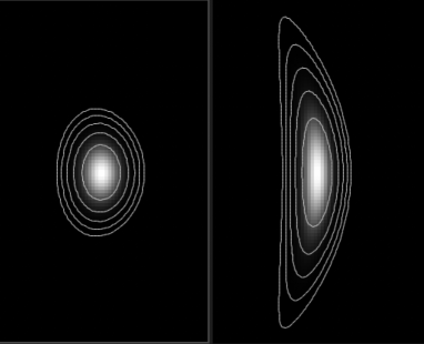
Figure 1: Gaussian images with the lensing distortion which is used in the simulation test in this paper. The left side image, weak arc(WA), is distorted by lensing distortion g=0.3𝑔0.3{\mbox{\boldmath$g$}}=-0.3, =0.0050.005{\mbox{\boldmath${\cal F}$}}=-0.005/pixels and 𝒢=0.005𝒢0.005{\mbox{\boldmath${\cal G}$}}=0.005/pixels, and the right image, strong arc(SA), is distorted by lensing distortion g=0.6𝑔0.6{\mbox{\boldmath$g$}}=-0.6, =0.010.01{\mbox{\boldmath${\cal F}$}}=-0.01/pixels and 𝒢=0.01𝒢0.01{\mbox{\boldmath${\cal G}$}}=0.01/pixels. The brightness of the image is linear scale, but the contour is log scale for visibility of arc shape.
Refer to caption
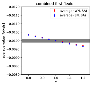
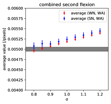
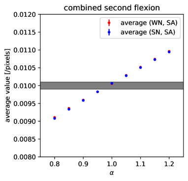
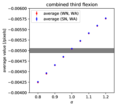
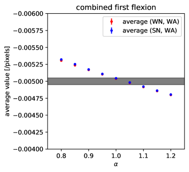
Figure 2: The average value of the combined first flexion in the simulation test with the first constraint condition. The horizontal axis is the parameter of the constraint condition α𝛼\alpha. The red and blue points mean the result of the data set (WN, WA) and (SN, WA) respectively; the detail of the set is described in the main text. The gray region means true flexion value with +/- 1% error. We can see the average values are strongly dependent on the constraint condition.

We calculate the value of the ensemble average of the three combined flexions using a simple simulated image and two constraint conditions. In this simulation we used a simple Gaussian image which has 4 pixels Gaussian radius. We make a lensed image by applying intrinsic and lensing distortions to the Gaussian image. We used two standard deviation sets as intrinsic distortions weak noise(WN) and strong noise(SN). The WN has noise with σg=0.2subscript𝜎𝑔0.2\sigma_{\mbox{\boldmath$g$}}=0.2, σ=0.001subscript𝜎0.001\sigma_{\mbox{\boldmath${\cal F}$}}=0.001/pixels(0.004 when convert to non-dimensional flexion NF with the Gaussian radius 4.0 pixels) and σ𝒢=0.001subscript𝜎𝒢0.001\sigma_{\mbox{\boldmath${\cal G}$}}=0.001/pixels(NF=0.004), and the SN has noise with σg=0.3subscript𝜎𝑔0.3\sigma_{\mbox{\boldmath$g$}}=0.3, σ=0.005subscript𝜎0.005\sigma_{\mbox{\boldmath${\cal F}$}}=0.005/pixels(NF=0.02) and σ𝒢=0.005subscript𝜎𝒢0.005\sigma_{\mbox{\boldmath${\cal G}$}}=0.005/pixels(NF=0.02). Then we used two lensing distortions, weak arc(WA) and strong arc(SA). The WA has distortion gL=0.3subscript𝑔𝐿0.3{\mbox{\boldmath$g$}}_{L}=-0.3, L=0.005subscript𝐿0.005{\mbox{\boldmath${\cal F}$}}_{L}=-0.005/pixels(NF=-0.02) and 𝒢L=0.005subscript𝒢𝐿0.005{\mbox{\boldmath${\cal G}$}}_{L}=0.005/pixels(NF=0.02), and The SA has distortion gL=0.6subscript𝑔𝐿0.6{\mbox{\boldmath$g$}}_{L}=-0.6, L=0.01subscript𝐿0.01{\mbox{\boldmath${\cal F}$}}_{L}=-0.01/pixels(NF=-0.04) and 𝒢L=0.01subscript𝒢𝐿0.01{\mbox{\boldmath${\cal G}$}}_{L}=0.01/pixels(NF=0.04). Figure 2 shows sample images which are Gaussian images distorted by only the lensing distortions, so this test investigates also the precision of flexion measurement from such an arc shape object.

A conjugate of the third flexion 𝓗Csubscript𝓗𝐶{\mbox{\boldmath${\cal H}$}}_{C} is equal to 𝓕Csubscript𝓕𝐶{\mbox{\boldmath${\cal F}$}}_{C} up to the first order, so the first one of the constraint condition we use in this simulation is

𝓗C=α𝓕Csubscript𝓗𝐶𝛼subscriptsuperscript𝓕𝐶\displaystyle{\mbox{\boldmath${\cal H}$}}_{C}=\alpha{\mbox{\boldmath${\cal F}$}}^{*}_{C} (26)

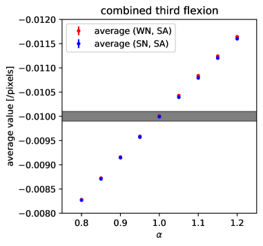
with variable α𝛼\alpha. Figure 2 to 8 show the ensemble average of the combined flexions for variable α𝛼\alpha of the constraint condition. Then, the second one of the constraint condition is simply applying constant for 𝓗Csubscript𝓗𝐶{\mbox{\boldmath${\cal H}$}}_{C}, so

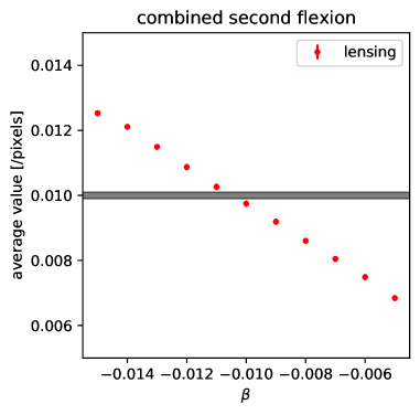
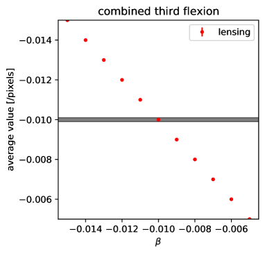
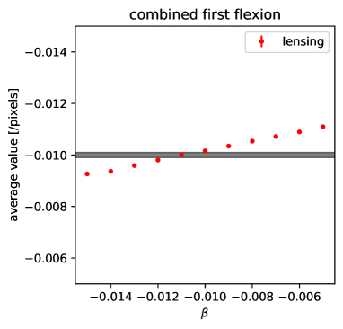
𝓗C=βsubscript𝓗𝐶𝛽\displaystyle{\mbox{\boldmath${\cal H}$}}_{C}=\beta (27)

Figure 8 to 10 show the ensemble average with variable β𝛽\beta of the constraint condition only for the data set (SN, SA). We can see the combined flexions strongly depend on not only strength of intrinsic noise but also selection of the constraint condition.
Refer to caption
Figure 3: Same plot as figure 2 except that the red and blue points are in the case of (WN, SA) and (SN, SA) respectively.
Refer to caption
Figure 4: Same plot as figure 2 except that the red and blue points are the average value of combined second flexion in the case of (WN, WA) and (SN, WA) respectively.
Refer to caption
Figure 5: Same plot as figure 4 except that the red and blue points are in the case of (WN, SA) and (SN, SA) respectively.
Refer to caption
Figure 6: Same plot as figure 2 except that the red and blue points are the average value of combined third flexion in the case of (WN, WA) and (SN, WA) respectively.
Refer to caption
Figure 7: Same plot as figure 6 except that the red and blue points are in the case of (WN, SA) and (SN, SA) respectively.
Refer to caption
Figure 8: The average value of the combined first flexion in the simulation test with the second constraint condition. The horizontal axis is the parameter of the constraint condition β𝛽\beta. The red points mean the result of the data set (SN, SA). The solid line is combined first flexion without any intrinsic distortions, so lensing first flexion. We can see the average values are strongly dependent on the constraint condition.
Refer to caption
Figure 9: Same plot as figure 8 except that the red points are the average value of combined second flexion.
Refer to caption
Figure 10: Same plot as figure 8 except that the red points are the average value of combined third flexion.

4 A new method for flexion precise measurement without intrinsic noise

4.1 eigen flexion values and lensing information

In the previous section, it was shown that systematic error occurs because of the wrong choice of the constraint condition, or the wrong choice of the quantities we measure. In fact it turns out that the latter is the case and we can find two kinds of combination of the combined flexions whose average is independent of the selection of the constraint condition. We call these combinations as eigen flexions.

In deriving the eigen flexions, we use the ERA method where the zero image in the zero plane has circular shape with arbitrary radial profile. This means that the brightness distribution of zero image is a function with variable |d𝜷~|2superscript𝑑~𝜷2|d{\tilde{{\bm{\beta}}}}|^{2}. Then the variable is transformed in the lens plane up to the first-order in flexion as

|d𝜷~|2superscript𝑑~𝜷2\displaystyle|d{\tilde{{\bm{\beta}}}}|^{2} =\displaystyle= (1κ)2|1+𝒈I𝒈L|2((1+|𝒈C|2)d𝜽022Re[𝒈Cd𝜽22]12(Re[𝓕Ed𝜽13]+Re[𝓖Ed𝜽33]))superscript1𝜅2superscript1subscript𝒈𝐼superscriptsubscript𝒈𝐿21superscriptsubscript𝒈𝐶2𝑑subscriptsuperscript𝜽202Redelimited-[]superscriptsubscript𝒈𝐶𝑑subscriptsuperscript𝜽2212Redelimited-[]superscriptsubscript𝓕𝐸𝑑subscriptsuperscript𝜽31Redelimited-[]superscriptsubscript𝓖𝐸𝑑subscriptsuperscript𝜽33\displaystyle\left(1-\kappa\right)^{2}\left|1+{\mbox{\boldmath$g$}}_{I}{\mbox{\boldmath$g$}}_{L}^{*}\right|^{2}\left(\left(1+|{\mbox{\boldmath$g$}}_{C}|^{2}\right)d{\bm{\theta}}^{2}_{0}-2{\rm Re}\left[{\mbox{\boldmath$g$}}_{C}^{*}d{\bm{\theta}}^{2}_{2}\right]-\frac{1}{2}\left({\rm Re}\left[{\mbox{\boldmath${\cal F}$}}_{E}^{*}d{\bm{\theta}}^{3}_{1}\right]+{\rm Re}\left[{\mbox{\boldmath${\cal G}$}}_{E}^{*}d{\bm{\theta}}^{3}_{3}\right]\right)\right) (28)
𝓕Esubscript𝓕𝐸\displaystyle{\mbox{\boldmath${\cal F}$}}_{E} \displaystyle\equiv 2𝓕C+𝓗C2𝒈C𝓕C𝒈C𝓖C2subscript𝓕𝐶subscriptsuperscript𝓗𝐶2subscript𝒈𝐶subscriptsuperscript𝓕𝐶subscriptsuperscript𝒈𝐶subscript𝓖𝐶\displaystyle 2{\mbox{\boldmath${\cal F}$}}_{C}+{\mbox{\boldmath${\cal H}$}}^{*}_{C}-2{\mbox{\boldmath$g$}}_{C}{\mbox{\boldmath${\cal F}$}}^{*}_{C}-{\mbox{\boldmath$g$}}^{*}_{C}{\mbox{\boldmath${\cal G}$}}_{C} (29)
𝓖Esubscript𝓖𝐸\displaystyle{\mbox{\boldmath${\cal G}$}}_{E} \displaystyle\equiv 𝓖C𝒈C𝓗Csubscript𝓖𝐶subscript𝒈𝐶subscriptsuperscript𝓗𝐶\displaystyle{\mbox{\boldmath${\cal G}$}}_{C}-{\mbox{\boldmath$g$}}_{C}{\mbox{\boldmath${\cal H}$}}^{*}_{C} (30)

Natural combinations of the combined flexions appear here. This equation means that the brightness distribution of the lensed image is a function with variables 𝒈Csubscript𝒈𝐶{\mbox{\boldmath$g$}}_{C}, 𝓕Esubscript𝓕𝐸{\mbox{\boldmath${\cal F}$}}_{E} and 𝓖Esubscript𝓖𝐸{\mbox{\boldmath${\cal G}$}}_{E}, and the flexion effect is described by 𝓕Esubscript𝓕𝐸{\mbox{\boldmath${\cal F}$}}_{E} and 𝓖Esubscript𝓖𝐸{\mbox{\boldmath${\cal G}$}}_{E}. We call these as eigen flexions.

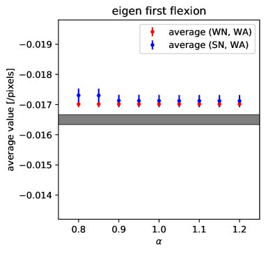
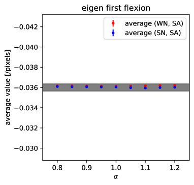
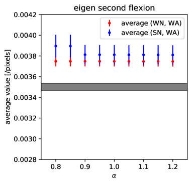
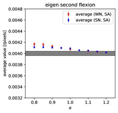
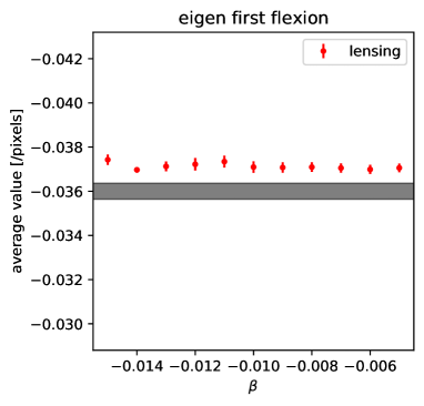
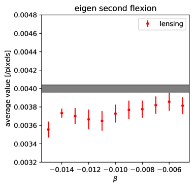
Using the simulation described in the previous section, we have confirmed the independence of the eigen flexion from the choice of the above two constraint conditions with the same simulation test as the previous section. ( Actually we have checked the independence of the result using other constraint conditions.) Figures 12 to 16 are the result of the simulation test. We can see the fluctuations of the average of the eigen flexion decrease compared to the average of the combined flexions. So, we can obtain the eigen flexion 𝓕Esubscript𝓕𝐸{\mbox{\boldmath${\cal F}$}}_{E} and 𝓖Esubscript𝓖𝐸{\mbox{\boldmath${\cal G}$}}_{E} by using arbitrary convenient value of the parameter in the constraint condition from the combined flexion 𝓕Csubscript𝓕𝐶{\mbox{\boldmath${\cal F}$}}_{C} and 𝓖Csubscript𝓖𝐶{\mbox{\boldmath${\cal G}$}}_{C}. However, because the eigen flexions still contain the intrinsic shear term |gI|2superscriptsubscript𝑔𝐼2|{\mbox{\boldmath$g$}}_{I}|^{2}, the ensemble average of the eigen flexions have systematic error due to intrinsic noise.

We have found a combination of eigen flexion which do not include |𝒈I|2superscriptsubscript𝒈𝐼2|{\mbox{\boldmath$g$}}_{I}|^{2} as follows

𝓕Esubscript𝓕superscript𝐸\displaystyle{\mbox{\boldmath${\cal F}$}}_{E^{\prime}} \displaystyle\equiv 𝓕E+𝒈C𝓖E+𝒈C𝓕E+𝒈C2𝓖E1|𝒈C|2=2𝓕C+𝓗C+𝒈C𝓗Csubscript𝓕𝐸subscriptsuperscript𝒈𝐶subscript𝓖𝐸subscript𝒈𝐶superscriptsubscript𝓕𝐸superscriptsubscript𝒈𝐶2superscriptsubscript𝓖𝐸1superscriptsubscript𝒈𝐶22subscript𝓕𝐶subscriptsuperscript𝓗𝐶subscript𝒈𝐶subscript𝓗𝐶\displaystyle\frac{{\mbox{\boldmath${\cal F}$}}_{E}+{\mbox{\boldmath$g$}}^{*}_{C}{\mbox{\boldmath${\cal G}$}}_{E}+{\mbox{\boldmath$g$}}_{C}{\mbox{\boldmath${\cal F}$}}_{E}^{*}+{\mbox{\boldmath$g$}}_{C}^{2}{\mbox{\boldmath${\cal G}$}}_{E}^{*}}{1-|{\mbox{\boldmath$g$}}_{C}|^{2}}=2{\mbox{\boldmath${\cal F}$}}_{C}+{\mbox{\boldmath${\cal H}$}}^{*}_{C}+{\mbox{\boldmath$g$}}_{C}{\mbox{\boldmath${\cal H}$}}_{C} (31)
𝓖Esubscript𝓖superscript𝐸\displaystyle{\mbox{\boldmath${\cal G}$}}_{E^{\prime}} \displaystyle\equiv 𝓖E+𝒈C𝓕E+𝒈C2𝓕E+𝒈C3𝓖E1|𝒈C|2=𝓖C+2𝒈C𝓕C+𝒈C2𝓗C.subscript𝓖𝐸subscript𝒈𝐶subscript𝓕𝐸subscriptsuperscript𝒈2𝐶superscriptsubscript𝓕𝐸subscriptsuperscript𝒈3𝐶superscriptsubscript𝓖𝐸1superscriptsubscript𝒈𝐶2subscript𝓖𝐶2subscript𝒈𝐶subscript𝓕𝐶subscriptsuperscript𝒈2𝐶subscript𝓗𝐶\displaystyle\frac{{\mbox{\boldmath${\cal G}$}}_{E}+{\mbox{\boldmath$g$}}_{C}{\mbox{\boldmath${\cal F}$}}_{E}+{\mbox{\boldmath$g$}}^{2}_{C}{\mbox{\boldmath${\cal F}$}}_{E}^{*}+{\mbox{\boldmath$g$}}^{3}_{C}{\mbox{\boldmath${\cal G}$}}_{E}^{*}}{1-|{\mbox{\boldmath$g$}}_{C}|^{2}}={\mbox{\boldmath${\cal G}$}}_{C}+2{\mbox{\boldmath$g$}}_{C}{\mbox{\boldmath${\cal F}$}}_{C}+{\mbox{\boldmath$g$}}^{2}_{C}{\mbox{\boldmath${\cal H}$}}_{C}. (32)

Finally, by taking ensemble average of them, we can remove intrinsic distortions,

𝓕Edelimited-⟨⟩subscript𝓕superscript𝐸\displaystyle\left<{\mbox{\boldmath${\cal F}$}}_{E^{\prime}}\right> =\displaystyle= 3𝓕L+𝒈L𝓕L3subscript𝓕𝐿subscript𝒈𝐿subscriptsuperscript𝓕𝐿\displaystyle 3{\mbox{\boldmath${\cal F}$}}_{L}+{\mbox{\boldmath$g$}}_{L}{\mbox{\boldmath${\cal F}$}}^{*}_{L} (33)
𝓖Edelimited-⟨⟩subscript𝓖superscript𝐸\displaystyle\left<{\mbox{\boldmath${\cal G}$}}_{E^{\prime}}\right> =\displaystyle= 𝓖L+2𝒈L𝓕L+𝒈L2𝓕L,subscript𝓖𝐿2subscript𝒈𝐿subscript𝓕𝐿subscriptsuperscript𝒈2𝐿subscriptsuperscript𝓕𝐿\displaystyle{\mbox{\boldmath${\cal G}$}}_{L}+2{\mbox{\boldmath$g$}}_{L}{\mbox{\boldmath${\cal F}$}}_{L}+{\mbox{\boldmath$g$}}^{2}_{L}{\mbox{\boldmath${\cal F}$}}^{*}_{L}, (34)

where we assume that the intrinsic distortions are independent of each other. Equation 33 and 34 still contain lensing shear 𝒈Lsubscript𝒈𝐿{\mbox{\boldmath$g$}}_{L}, but it can be obtained by ensemble average of combined shear 𝒈Csubscript𝒈𝐶{\mbox{\boldmath$g$}}_{C}. We call the two flexions 𝓕Edelimited-⟨⟩subscript𝓕superscript𝐸\left<{\mbox{\boldmath${\cal F}$}}_{E^{\prime}}\right> and 𝓖Edelimited-⟨⟩subscript𝓖superscript𝐸\left<{\mbox{\boldmath${\cal G}$}}_{E^{\prime}}\right> as an eigen (first and second) flexion combination.

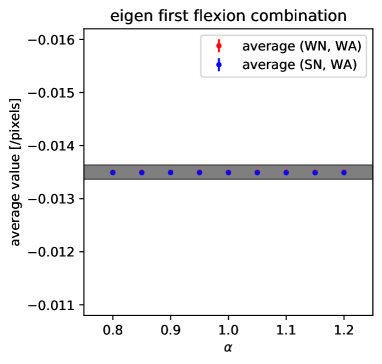
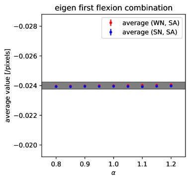
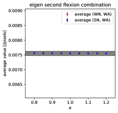
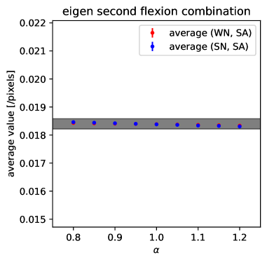
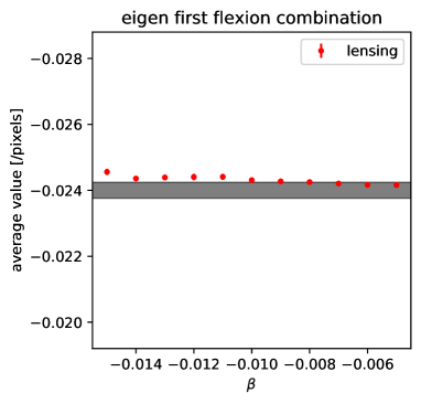
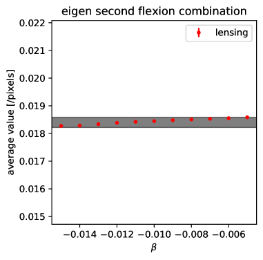
We investigate the eigen flexion combinations by the same simulation in the combined flexions. Figures 18 to 22 are plots of the ensemble average of the eigen flexion combinations measured from the simulated images. We can see the average value does not depend on the strength of intrinsic distortions, so the their average values have only the lensing information and coincide correctly with the given values.

It is confirmed that the ensemble average of the eigen flexion combinations have only lensing information, so finally, after obtaining 𝒈Lsubscript𝒈𝐿{\mbox{\boldmath$g$}}_{L} from 𝒈Cdelimited-⟨⟩subscript𝒈𝐶\left<{\mbox{\boldmath$g$}}_{C}\right>, we can obtain weak gravitational lensing flexions as

𝓕Lsubscript𝓕𝐿\displaystyle{\mbox{\boldmath${\cal F}$}}_{L} =\displaystyle= 3𝓕E𝒈C𝓕E9|𝒈C|23delimited-⟨⟩subscript𝓕superscript𝐸delimited-⟨⟩subscript𝒈𝐶superscriptdelimited-⟨⟩subscript𝓕superscript𝐸9superscriptdelimited-⟨⟩subscript𝒈𝐶2\displaystyle\frac{3\left<{\mbox{\boldmath${\cal F}$}}_{E^{\prime}}\right>-\left<{\mbox{\boldmath$g$}}_{C}\right>\left<{\mbox{\boldmath${\cal F}$}}_{E^{\prime}}\right>^{*}}{9-|\left<{\mbox{\boldmath$g$}}_{C}\right>|^{2}} (35)
𝓖Lsubscript𝓖𝐿\displaystyle{\mbox{\boldmath${\cal G}$}}_{L} =\displaystyle= 𝓖E𝒈C(6|𝒈C|2)𝓕E+𝒈C𝓕E9|𝒈C|2,delimited-⟨⟩subscript𝓖superscript𝐸delimited-⟨⟩subscript𝒈𝐶6superscriptdelimited-⟨⟩subscript𝒈𝐶2delimited-⟨⟩subscript𝓕superscript𝐸delimited-⟨⟩subscript𝒈𝐶superscriptdelimited-⟨⟩subscript𝓕superscript𝐸9superscriptdelimited-⟨⟩subscript𝒈𝐶2\displaystyle\left<{\mbox{\boldmath${\cal G}$}}_{E^{\prime}}\right>-\left<{\mbox{\boldmath$g$}}_{C}\right>\frac{\left(6-|\left<{\mbox{\boldmath$g$}}_{C}\right>|^{2}\right)\left<{\mbox{\boldmath${\cal F}$}}_{E^{\prime}}\right>+\left<{\mbox{\boldmath$g$}}_{C}\right>\left<{\mbox{\boldmath${\cal F}$}}_{E^{\prime}}\right>^{*}}{9-|\left<{\mbox{\boldmath$g$}}_{C}\right>|^{2}}, (36)
Refer to caption
Figure 11: Same plot as figure 2 except that the red and blue points are the average value of eigen first flexion. We can see fluctuation of the average value decreases compare to the average of combined first flexion in all α𝛼\alpha region.
Refer to caption
Figure 12: Same plot as figure 12 except that the red and blue points are in the case of (WN, SA) and (SN, SA) respectively.
Refer to caption
Figure 13: Same plot as figure 12 except that the red and blue points are the average value of eigen second flexion.
Refer to caption
Figure 14: Same plot as figure 14 except that the red and blue points are in the case of (WN, SA) and (SN, SA) respectively.
Refer to caption
Figure 15: Same plot as figure 12 except using the second constraint condition, the horizontal axis means the constant constraint condition β𝛽\beta and points are only (SN, SA).
Refer to caption
Figure 16: Same plot as figure 16 except that the red points are the average value of eigen second flexion.
Refer to caption
Figure 17: Same plot as figure 2 except that the red and blue points are the average value of eigen first flexion combination. We can see the average values have same value as lensing value in all α𝛼\alpha range.
Refer to caption
Figure 18: Same plot as figure 18 except that the red and blue points are in the case of (WN, SA) and (SN, SA) respectively.
Refer to caption
Figure 19: Same plot as figure 18 except that the red and blue points are the average value of eigen second flexion complex.
Refer to caption
Figure 20: Same plot as figure 20 except that the red and blue points are the average value of eigen second flexion.
Refer to caption
Figure 21: Same plot as figure 18 except using the second constraint condition, the horizontal axis means the constant constraint condition β𝛽\beta and points are only (SN, SA).
Refer to caption
Figure 22: Same plot as figure 16 except that the red points are the average value of eigen second flexion combination.

At the end of this section, we summarize the steps to measure weak lensing flexion. The all steps for measuring the lensing flexions are as follows, and figure 23 shows the relations between all kinds of the flexions.

The first step is to decide the constraint condition which constrains the relation between the combined first flexion and the combined third flexion. Although the condition can be chosen from many possibilities, the condition we used in the simulation data, C=Csubscript𝐶superscriptsubscript𝐶{\mbox{\boldmath${\cal F}$}}_{C}={\mbox{\boldmath${\cal H}$}}_{C}^{*}, seems reasonable because of its simplicity as well as the result of the simulation test.

The second step is to measure the zero moments of the object image. The zero moments are image moments of the object which are defined to have zero value if the spin number of the moments is not zero. The formalism of the zero moments is defined in the zero plane and it has been transformed in the image plane(equation 25). Thus, the zero moments can be determined in the image plane, by measuring five shape parameters of the observed image [centroid, combined shear, three combined flexions] and then by using the constraint equation we can make the four zero moments [11subscriptsuperscript11{\cal M}^{1}_{1}, 22subscriptsuperscript22{\cal M}^{2}_{2}, 13subscriptsuperscript31{\cal M}^{3}_{1}, 33subscriptsuperscript33{\cal M}^{3}_{3}] zero.

The third step is to calculate the eigen flexion combination. The combined flexions measured above depend on the constraint condition and include the intrinsic shear terms, so it is needed to calculate the eigen flexion combinations (equations 29, 30, 31 and 32) to obtain weak lensing flexions precisely.

The final step is to average of the eigen flexion combinations to obtain weak lensing flexions. The average value is obtained as a combination of lensing shear and lensing flexions (equations 33 and 34), so the lensing flexions are obtained by the inverse transformation(equations 35 and 36) after obtaining lensing shear from average of the combined shear, gL=gCsubscript𝑔𝐿delimited-⟨⟩subscript𝑔𝐶{\mbox{\boldmath$g$}}_{L}=\left<{\mbox{\boldmath$g$}}_{C}\right>.

Refer to caption
Figure 23: The relations between all kinds of the flexions in the steps for measuring the lensing flexions.

4.2 Comparison with HOLICs method

In this section, we compare the precision of the new flexion measurement method with the HOLICs method which was developed before by us. The details of the HOLICs method can be seen in Okura, Umetsu and Futamase 2007 and 2008.

Because the HOLICs method does not consider the third flexion (equation 24), to investigate the difference of pure shape measurement error, we compare the two methods with a simple situation that has only lensing distortion. We made four simulation images with Gaussian profile and Gaussian radius = 4 pixels and distorted them with a different distortion set. The each distortion set have distortion parameters as the first flexion only(𝒈L=0.0subscript𝒈𝐿0.0{\mbox{\boldmath$g$}}_{L}=0.0, 𝓖L=0.0subscript𝓖𝐿0.0{\mbox{\boldmath${\cal G}$}}_{L}=0.0: "F only"), the second flexion only(𝒈L=0.0subscript𝒈𝐿0.0{\mbox{\boldmath$g$}}_{L}=0.0, 𝓕L=0.0subscript𝓕𝐿0.0{\mbox{\boldmath${\cal F}$}}_{L}=0.0: "G only"), the first flexion with ellipticity(𝒈L=0.3subscript𝒈𝐿0.3{\mbox{\boldmath$g$}}_{L}=-0.3, 𝓖L=0.0subscript𝓖𝐿0.0{\mbox{\boldmath${\cal G}$}}_{L}=0.0: "F and g") and the second flexion with ellipticity(𝒈L=0.3subscript𝒈𝐿0.3{\mbox{\boldmath$g$}}_{L}=-0.3, 𝓕L=0.0subscript𝓕𝐿0.0{\mbox{\boldmath${\cal F}$}}_{L}=0.0: "G and g"). The precisions of each method are compared with the error ratio 𝓕esubscript𝓕𝑒{\mbox{\boldmath${\cal F}$}}_{e} or 𝓖esubscript𝓖𝑒{\mbox{\boldmath${\cal G}$}}_{e} of flexion measurement, the error ratio is defined from the true value 𝓕Lsubscript𝓕𝐿{\mbox{\boldmath${\cal F}$}}_{L} or 𝓖Lsubscript𝓖𝐿{\mbox{\boldmath${\cal G}$}}_{L} used for making the simulation image and measured value 𝓕msubscript𝓕𝑚{\mbox{\boldmath${\cal F}$}}_{m} or 𝓖msubscript𝓖𝑚{\mbox{\boldmath${\cal G}$}}_{m} as

𝓕esubscript𝓕𝑒\displaystyle{\mbox{\boldmath${\cal F}$}}_{e} =\displaystyle= |𝓕m𝓕L𝓕L|subscript𝓕𝑚subscript𝓕𝐿subscript𝓕𝐿\displaystyle\left|\frac{{\mbox{\boldmath${\cal F}$}}_{m}-{\mbox{\boldmath${\cal F}$}}_{L}}{{\mbox{\boldmath${\cal F}$}}_{L}}\right| (37)
𝓖esubscript𝓖𝑒\displaystyle{\mbox{\boldmath${\cal G}$}}_{e} =\displaystyle= |𝓖m𝓖L𝓖L|.subscript𝓖𝑚subscript𝓖𝐿subscript𝓖𝐿\displaystyle\left|\frac{{\mbox{\boldmath${\cal G}$}}_{m}-{\mbox{\boldmath${\cal G}$}}_{L}}{{\mbox{\boldmath${\cal G}$}}_{L}}\right|. (38)

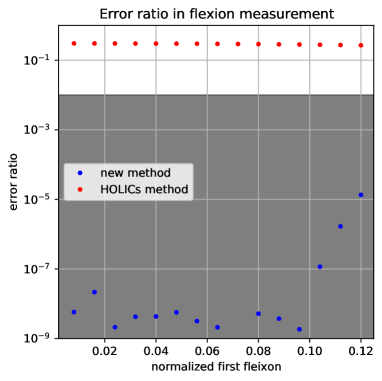
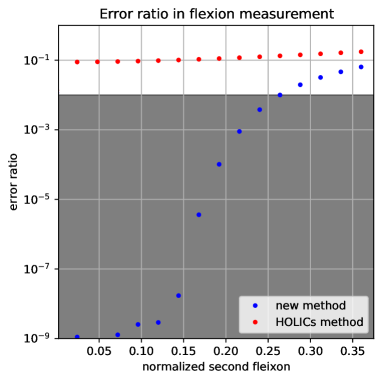
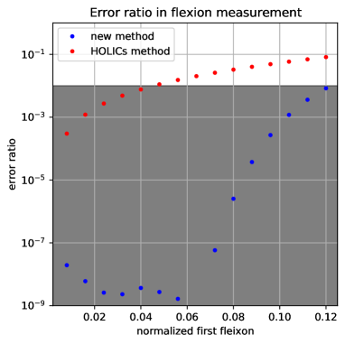
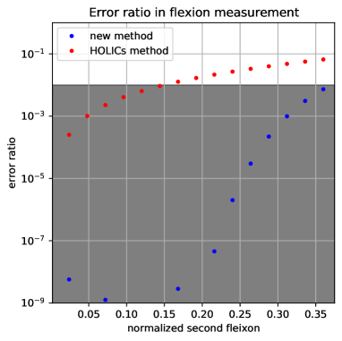
The figure 25 and 25 show the result of the comparison with the distortion set "F only" and "G only". We can see the error ratio of the new method is very small even in a strong flexion region which makes the error ratio more than 1% in the HOLICs method. The figure 27 and 27 show the result of the comparison with the distortion set "F and g" and "G and g". We can see the HOLICs method has a large error ratio even in weak flexion limits, because the HOLICs method does not consider the combination of shear and flexion. However, the new method has a very small error ratio even when shear and flexion are combined, because the new method considers the effect from shear in flexion measurement. These results show clearly that the new method is an improved method much from the HOLICs method.
Refer to caption
Figure 24: The error ratio of the first flexion measurement for distortion set "F only". The horizontal axis means the normalized input first flexion which is defined the products of the input first flexion 𝓕tsubscript𝓕𝑡{\mbox{\boldmath${\cal F}$}}_{t}[/pixels] and the Gaussian radius of the simulated image rg=4subscript𝑟𝑔4r_{g}=4[pixels] , and the vertical axis means the error ratio 𝓕esubscript𝓕𝑒{\mbox{\boldmath${\cal F}$}}_{e}, and the gray region means the error ratio is under 1%. The blue points mean the new method and the red points mean the HOLICs method.
Refer to caption
Figure 25: Same plot as figure 25 except that the vertical axis means the error ratio of the second flexion measurement for distortion set "G only" and the horizontal axis means the normalized input second flexion 𝓖tsubscript𝓖𝑡{\mbox{\boldmath${\cal G}$}}_{t}.
Refer to caption
Figure 26: Same plot as figure 25 except that the vertical axis means the error ratio of the second flexion measurement for distortion set "F and g" and the horizontal axis means the normalized input second flexion 𝓕tsubscript𝓕𝑡{\mbox{\boldmath${\cal F}$}}_{t}.
Refer to caption
Figure 27: Same plot as figure 25 except that the vertical axis means the error ratio of the second flexion measurement for distortion set "G and g" and the horizontal axis means the normalized input second flexion 𝓖tsubscript𝓖𝑡{\mbox{\boldmath${\cal G}$}}_{t}.

5 Summary

In this paper, we developed a new precise flexions measurement method. Flexions appeared in third order terms in the expansion of the lensing equation than shear, so the formulas to measure flexions are much more complicated than that of shear.

We applied the idea of the zero plane to calculate the relation between the image plane and the zero plane. In the course of derivation, we have a third type of flexion which is independent from the first and the second flexions. This causes a very serious problem, because the addition of independent parameters makes it impossible to measure the three flexions uniquely. So we have to use some constraint condition to determine uniquely flexion, but it means the measured flexion and average of the flexion depend on the selection of the constraint condition. We found that the distorted image from circular shape has only two combinations of combined flexions, called eigen flexions. It is found that the eigen flexion is independent from the constraint condition. But the average of the eigen flexion includes intrinsic noise which cannot be eliminated by averaging. We then constructed the combinations of eigen flexions called eigen flexion combinations which contain only linear terms of the intrinsic distortion. After averaging the eigen flexion combination the dependence on the intrinsic value can be eliminated. The average of the new combinations still contain the lensing shear but it can be obtained from the average of the combined shear. We confirmed using a simple numerical simulation that the average of the eigen flexion combination do not depend on the choice of the constraint and are free from the intrinsic noise.

In this way we have developed a method which can measure the lensing flexion by measuring shape of galaxy image, but there are other effects in real observation which change the shape of the image on the top of the lensed image. We need to correct them to have the lensed image before applying the method of flexion analysis developed above. One of the most important corrections is PFS correction which we will study in the next paper.

Appendix A Additional mask for moment measurement

In this section we explain about the additional mask for weight function in moment measurement.

As we explained in section 2.3, a weight function which is defined as a circular function in the zero plane is used for the moment measurement. The variable of the weight function is simply |d𝜷~|𝑑~𝜷|d{\tilde{{\bm{\beta}}}}| in the zero plane, but it has nonlinear terms in the image plane and the terms make the distribution of the weight function a very complicated. The left image of figure 28 and figure 29 are Gaussian weight functions in the image plane with flexion distortions. We can see there are some peaks in the outer part from the central peak where the object is located. If there are other objects on the peaks, the weak lensing information can not be obtained correctly. The peaks appear even in weak flexion limits. Because the position of the peaks has a tendency to be far from the object in weak flexion and close to the object in stronger flexion, so in some situations, e.g. weak flexion or taking a small stamp for the object, it may be able to be ignored, however it is clear that the peaks can be ignored in all cases of future shape measurement. One of the reliable techniques to remove the peak is using a mask for the weight function. Because the peaks are in the outer region with δ𝜷~(𝜽)d𝜽>0𝛿~𝜷𝜽𝑑𝜽0{\delta{\tilde{{\bm{\beta}}}}({\bm{\theta}})\cdot d{\bm{\theta}}}>0, the appropriate mask M(𝜽)𝑀𝜽M({\bm{\theta}}) can be obtained as

M(𝜽)𝑀𝜽\displaystyle M({\bm{\theta}}) \displaystyle\equiv H(δ𝜷~(𝜽)d𝜽)𝐻𝛿~𝜷𝜽𝑑𝜽\displaystyle H\left(\delta{\tilde{{\bm{\beta}}}}({\bm{\theta}})\cdot d{\bm{\theta}}\right) (39)
δ𝜷~(𝜽)𝛿~𝜷𝜽\displaystyle\delta{\tilde{{\bm{\beta}}}}({\bm{\theta}}) \displaystyle\equiv (d𝜷~)(d𝜽)d𝜽+(d𝜷~)(d𝜽)d𝜽,𝑑~𝜷𝑑𝜽𝑑𝜽𝑑~𝜷𝑑superscript𝜽𝑑superscript𝜽\displaystyle{\frac{\partial{\left(d{\tilde{{\bm{\beta}}}}\right)}}{\partial{\left(d{\bm{\theta}}\right)}}}d{\bm{\theta}}+{\frac{\partial{\left(d{\tilde{{\bm{\beta}}}}\right)}}{\partial{\left(d{\bm{\theta}}^{*}\right)}}}d{\bm{\theta}}^{*}, (40)

where H𝐻H is Heaviside step function. The center images of the figures are the mask regions calculated using equation 39, then the right images of the figures are masked weight. We can see the Masked weight can mask the peaks.

Refer to caption
Figure 28: Weight(left), mask(center) and masked weight(right) region for image with 2nd flexion only. The black region in the center image is a masked region.
Refer to caption
Figure 29: Same image as figure 28 except the distortion is shear and both flexions.

Data availability

The simulation data underlying this article were created my original python codes, so these are available on request.

Acknowledgements

This work is supported in part by a Grant-in-Aid for Science Research from JSPS (No.20K03937 to T.F).

References

  • (1) Bacon, D. J., et al., 2006, MNRAS, 365, 414–428
  • (2) Bacon, D. J., et al., 2010, MNRAS, 409, 389–395
  • (3) Bird, J. P. and Goldberg, D. M., 2018, MNRAS, 476, 1198–1212
  • (4) Benjamin, C., Marusa, B., Rebecca, L., 2016, MNRAS, 463, 4287–4300
  • (5) Irwin, J. and Shmakova, M., 2006, ApJ, 645, 17–43, 2006
  • (6) Irwin, J., et al. 2007, Apj, 671, 1182-1195
  • (7) Joseph, M. F., et al., 2020, MNRAS, 501, 4103–4109
  • (8) Lanusse, F., 2016, A&A, 591, A2
  • (9) Leonard, A., et al. 2009, MNRAS, 395, 1438–1448
  • (10) Levinson, R., 2013, PASP, 125, 1474–1495
  • (11) Goldberg, D. M., and Bacon, D. J., 2005, ApJ, 619, 741–748
  • (12) Goldberg, D. M., and Leonard, A., 2007, ApJ, 660, 1003-1015
  • (13) Goldberg, D. M., and Natarajan, P., 2002, ApJ, 564, 65-72
  • (14) Miller, L., et al., 2007, MNRAS, 382 185
  • (15) Munshi, D., Valagesas P., Van Waerbeke, L. & Heavens, A., 2008, Phys. Rept. 462, 67
  • (16) Okura, Y., Umetsu, K. and Futamase, T., 2007, 660, 995-1002
  • (17) Okura, Y., Umetsu, K. and Futamase, T., 2008, 680, 1-16
  • (18) Okura, Y., Futamase, T., 2011, ApJ, 730, 9
  • (19) Okura, Y., Futamase, T., 2012, ApJ, 748, 112
  • (20) Okura, Y., Futamase, T., 2013, ApJ, 771, 37
  • (21) Okura, Y., Futamase, T., 2014, ApJ, 792, 104
  • (22) Okura, Y., Futamase, T., 2015, A&A, 576, 63
  • (23) Okura, Y., Futamase, T., 2016, ApJ, 827, 138
  • (24) Okura, Y., Futamase, T., 2018, MNRAS, 479, 4971–4983
  • (25) Schneider., 2006, Part 1: Introduction to gravitational lensing and cosmology, ISBN: 3-540-30309-X
  • (26) Cardone, V. F., et al., 2016, MNRAS, 462, 4028–4037