Determination of Sodium Abundance Ratio from Low-Resolution Stellar Spectra and Its Applications

Abstract

We present a method to determine sodium-abundance ratios ([Na/Fe]) using the Na I D doublet lines in low-resolution ($R\sim$ 2000) stellar spectra. As stellar Na I D lines are blended with those produced by the interstellar medium (ISM), we developed a technique for removing the interstellar Na I D lines using the relationship between extinction, which is proportional to $E(B-V)$, and the equivalent width (EW) of the interstellar Na I D absorption lines. When measuring [Na/Fe], we also considered corrections for non-local thermodynamic equilibrium (NLTE) effects. Comparisons with data from high-resolution spectroscopic surveys suggest that the expected precision of [Na/Fe] from low-resolution spectra is better than 0.3 dex for stars with [Fe/H] $>$ –3.0. We also present a simple application employing the estimated [Na/Fe] values for a large number of stellar spectra from the Sloan Digital Sky Survey (SDSS). After classifying the SDSS stars into Na-normal, Na-high, and Na-extreme, we explore their relation to stars in Galactic globular clusters (GCs). We find that, while the Na-high SDSS stars exhibit a similar metallicity distribution function (MDF) to that of the GCs, indicating that the majority of such stars may have originated from GC debris, the MDF of the Na-normal SDSS stars follows that of typical disk and halo stars. As there is a high fraction of carbon-enhanced metal-poor stars among the Na-extreme stars, they may have a non-GC origin, perhaps due to mass-transfer events from evolved binary companions.

1. Introduction

A non-zero fraction of field stars in the Milky Way (MW) are known to exhibit large abundances of light elements such as N, Na, and Al (Carretta et al., 2010; Fernández-Trincado et al., 2016; Martell et al., 2016; Schiavon et al., 2017a; Pereira et al., 2019). Globular clusters (GCs) in the MW also display significant abundance variations of the light elements, as well as strong anti-correlations between the abundances of Na and O, N and C, and Al and Mg (Carretta et al., 2009), which numerous authors have taken to be associated with the existence of multiple populations of (first- and second-generation) stars in GCs.

Because the second-generation stars in MW GCs exhibit relatively high abundances of N, Na, and Al, the field stars enhanced with such elements are often regarded as objects that have been accreted from tidally disrupted GCs (Carretta et al., 2009; Carretta, 2016; Martell et al., 2016; Schiavon et al., 2017a; Horta et al., 2021; Tang et al., 2021). From this perspective, it is expected that the debris from partially or fully disrupted GCs contributed in some degree to the build-up of the Galactic halo (Thomas et al., 2020; Wan et al., 2020) and bulge (Lee et al., 2019; Lim et al., 2021), in addition to stars accreted from major and minor merger events such as Gaia-Sausage (GS; Belokurov et al., 2018), Gaia-Enceladus (GE; Helmi et al., 2018), Sequioa (Myeong et al., 2019), Thamnos 1 & 2 (Koppelman et al., 2019), and the currently disrupting Sagittarius dwarf galaxy (Ibata et al., 1994; Majewski et al., 2003).

Several previous studies have been carried out to evaluate the significance of the contribution of the GC-origin stars to the Galactic halo. For example, Martell & Grebel (2010) searched for halo giants that originated from GCs by identifying N-rich stars on the basis of CN-band strengths in low-resolution stellar spectra from the Sloan Digital Sky Survey (SDSS; York et al. 2000), in particular the stellar specific sub-survey Sloan Extension for Galactic Understanding and Exploration (SEGUE; Yanny et al. 2009), and reported a fraction of 2.5% of N-rich stars in the halo populations. Horta et al. (2021) also attempted to estimate the contribution of the GCs to the halo using the nitrogen abundances of giant stars from the Apache Point Observatory Galactic Evolution Experiment (APOGEE; Majewski et al., 2017), and derived a similar fraction, 2.7%.

In addition to N, Na has become a key element for recognizing the population of stars that have escaped from MW GCs and to estimate the contribution of the GC-origin stars in the local halo, as it is relatively straightforward to measure its abundance in optical and near-IR spectra for dwarfs and giants. The Galactic field halo stars usually have sodium-abundance ratios ([Na/Fe]) in the range $-0.5\lesssim{\rm[Na/Fe]}\lesssim+0.5$ (Suda et al., 2008), while higher abundance ratios are observed among members of the Galactic GCs (Carretta et al., 2010). Based on these results, several studies (Carretta et al., 2010; Martell et al., 2011; Ramírez et al., 2012) attempted to estimate the fraction of the Na-rich stars in the MW halo, reporting fractions from 2.8% to 17%. The clear interpretation is that there is a non-negligible contribution of disrupted GCs to the assembly of the Galactic halo. However, since most of these studies are based on small numbers of relatively bright stars (with [Na/Fe] obtained from high-resolution spectroscopy), they are limited to relatively local samples. In order to obtain a better understanding of the connection of the GC debris to the assembly of the Galactic halo, it is necessary to study a much large number of homogeneously analyzed stars reaching farther into the Galactic halo.

Fortunately, spectroscopic surveys such as legacy SDSS, SEGUE, and the Large Sky Area Multi-Object Fiber Spectroscopic Telescope (LAMOST; Cui et al., 2012) provide unprecedented numbers of stellar spectra, with resolution sufficiently high to identify the Na I D resonance lines. However, in order to estimate [Na/Fe] from a low-resolution stellar spectrum, one challenge is the presence of sodium from the integrated interstellar medium (ISM) between the Earth and the stars. The Na I D lines produced in the stellar atmosphere are blended with those from Na in the ISM, and they are not easily distinguishable. As a result, the Na I D lines in a low-resolution spectrum appear stronger than the intrinsic lines, and [Na/Fe] is generally over-estimated; the problem becomes even more severe at low Galactic latitudes. Note that throughout this paper, we refer to the Na I D lines produced by Na in the ISM as interstellar sodium (ISS) lines.

However, if one can remove the effects of ISS lines in a low-resolution spectrum, it is possible to obtain reasonably well-determined [Na/Fe] for very large numbers of stellar spectra from SDSS and LAMOST. In this paper, we collectively refer to all of the stellar spectra from SDSS, SEGUE, Baryon Oscillation Spectroscopic Survey (BOSS; Dawson et al., 2013), and extended Baryon Oscillation Spectroscopic Survey (eBOSS; Blanton et al., 2017) as SDSS stars. Based on these large samples, one can better understand the distribution and properties of the Na-rich stars and their relationship to MW GCs, and derive statistically well-estimated fractions of these stars in the Galactic halo. This paper presents a method for removing the effect of ISS from low-resolution SDSS stellar spectra, and determine estimates of their [Na/Fe] abundance ratios.

This paper is organized as follows. Section 2 describes the method for the removal of the ISS lines from the SDSS spectra and the determination of [Na/Fe]. Validation of the estimated [Na/Fe] ratios, along with systematic and random errors, and the impact of the signal-to-noise ratio (SNR) of a stellar spectrum on the measured [Na/Fe], are presented in Section 3. In Section 4, we present one application of sodium-abundance ratios to understand their linkage with GC debris. A summary is given in Section 5.

2. Methodology for Estimation of [Na/Fe]

2.1. Impacts of Interstellar Sodium Absorption

As stellar light travels through interstellar space, its intensity is attenuated by absorption or scattering by the ISM. As one result, in particular for certain chemical elements (e.g., Na and Ca), we expect ISM lines to be present in a stellar spectrum. The strength of these lines is correlated with the amount of dust or gas along the line-of-sight. The absorption lines produced by the ISM are normally narrow and sharp due to the small internal velocity dispersion of gas in the ISM. Thus, we can identify and remove them from the spectrum of an astronomical object with relatively small differences in the radial velocities between the object and the ISM gas clouds, especially for high-resolution spectra.

However, at low resolution, such as for SDSS stellar spectra, the stellar absorption lines are blended with the ISM absorption lines. In this case, they are not easily distinguishable from the intrinsic stellar lines, even for a relatively high-velocity star. When measuring the abundance of a given chemical element, the overall effect of the unresolved ISM lines is to produce an over-estimate of the stellar elemental abundance. Sodium is a classic example of this difficulty in optical spectra.

The impact of the ISS lines on a stellar spectrum is illustrated in Figure 1. The top-left panel of Figure 1 displays a high-resolution spectrum in the Na I D doublet region of the extremely metal-poor star BD+44^∘ 493, which was observed with Gemini/GRACES (Chene et al., 2014). From inspection, one can easily identify the strong ISS lines shifted to the red by about 3 Å from the weaker stellar lines. The red spectrum in the bottom-left panel shows a degraded version (to the SDSS resolving power of about $R\sim 2000$) of the high-resolution spectrum; the stellar and the ISS lines are indistinguishable. The top-right panel of the figure exhibits the high-resolution spectrum after excising the ISS lines; the bottom-right panel shows the degraded spectrum (red line). We clearly see the much weaker strength of the intrinsic lines compared to the ISS lines. The blue spectrum in the panels is a synthetic one generated with the stellar parameters ($T_{\rm{eff}}$ = 5430 K, log $g$ = 3.4, and [Fe/H] = –3.8) and sodium-abundance ratio ([Na/Fe] = +0.3), reported by Ito et al. (2013). Comparison of the bottom-left and bottom-right panels makes it obvious that the sodium-abundance ratio determined from low-resolution stellar spectra would result in a gross over-estimation without accounting for the presence of the ISS lines.

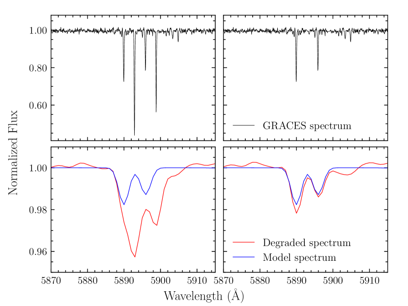
Figure 1.— Example spectra of the Na I D doublet region before (left column) and after (right column) removal of the ISS lines for the star BD$+$44^∘ 493. The upper panels show a high-resolution ($R$ = 45,000) spectrum obtained with Gemini/GRACES, whereas the red spectra in the bottom panels show its degraded spectrum to $R$ = 2000. The blue line is the synthetic spectrum generated with $T_{\rm{eff}}$ = 5430 K, log $g$ = 3.4, [Fe/H] = –3.8, and [Na/Fe] = 0.3, derived from the high-resolution spectroscopic analysis of this star by Ito et al. (2013).

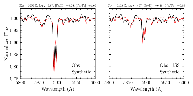
Figure 2.— An example of our ISS line-removal method applied to the spectrum of an SDSS star (J185226.5$+$201240). The left panel shows the spectrum before the removal of the ISS lines, while the right panel illustrates the spectrum after their removal. The black line indicates the observed spectrum; the red lines are the best-matching synthetic spectrum. The stellar parameters from the SSPP and [Na/Fe] (derived from the best-matching synthetic spectrum) are listed at the top of each panel. The much higher sodium-abundance ratio (by 1.0 dex) for the spectrum without removal of the the ISS lines is evident.

2.2. Removal of Interstellar Sodium Absorption

As demonstrated above, the removal of the Na I D lines produced by ISM is straightforward for high-resolution spectra, since we can easily identify the lines and excise them. In the case of low-resolution spectra, the situation is more complicated because the ISS lines are unresolved. Therefore, we require a method for eliminating the ISS lines before the estimation of [Na/Fe], and have developed the following approach.

We first estimated the strength of the ISS lines in terms of the expected equivalent width (EW) along the line-of-sight to a given star, and subtracted it from the measured Na I D lines present in a stellar spectrum. In order to calculate the EW of the ISS lines at a given Galactic coordinate, we adopted from the literature the relations between the reddening, $E(B-V)$, and the strength of the Na I D absorption lines by the ISM. Poznanski et al. (2012) derived a correlation between the reddening estimated by Schlegel et al. (1998) and the EW of the ISS lines, using high-resolution spectra of quasars (QSOs) and low-resolution spectra of QSOs and galaxies obtained by SDSS. Murga et al. (2015) also presented a relation between the reddening and the strength of the interstellar absorption of the Na I D and Ca II H & K lines, which were derived using extra-galactic sources from SDSS. They provide a best-fit relation for the range of $0\leq E(B-V)<0.08$. We employed the results from both studies. For stars with $0\leq E(B-V)<0.08$ we adopted the relation of Murga et al. (2015):

$$\mathrm{EW}(E(B-V))_{\rm{D2}}=\left(\frac{E(B-V)}{0.39}\right)^{0.63}\,\mathrm{\AA}$$

$$\mathrm{EW}(E(B-V))_{\rm{D1}}=\left(\frac{E(B-V)}{0.26}\right)^{1.06}\,\mathrm{\AA}$$

For stars with $E(B-V)\geq 0.08$ we adopt the relation of Poznanski et al. (2012):

$$\mathrm{EW}(E(B-V))_{\rm{D2}}=\frac{\mathrm{log_{10}}(E(B-V))+1.91}{2.16}\,\mathrm{\AA}$$

$$\mathrm{EW}(E(B-V))_{\rm{D1}}=\frac{\mathrm{log_{10}}(E(B-V))+1.76}{2.47}\,\mathrm{\AA}.$$

The subscript D1 in the equations indicates the Na I D line at 5896 Å, while D2 applies for the line at 5890 Å.

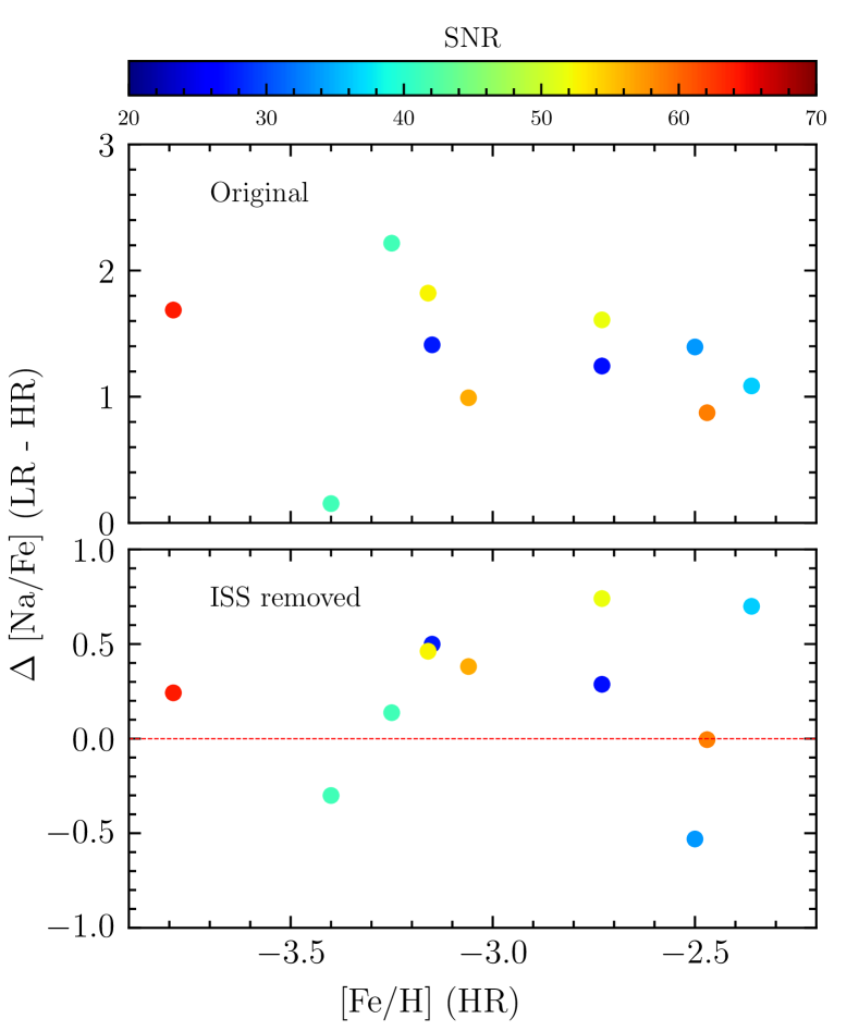
Figure 3.— Comparison of [Na/Fe] determined from the high-resolution (HR) analysis to that from our analysis of the degraded low-resolution (LR) spectrum before (upper panel) and after (lower panel) the ISS line removal. To remove the ISS lines, we first measured their EWs in the original high-resolution spectrum, and derived the Gaussian line profiles by following the method described in Section 2.2. The derived line profiles were degraded and subtracted from the degraded high-resolution spectrum to obtain a LR spectrum with the ISS lines removed. The color bar at the top represents the SNR of the high-resolution spectrum. It is clear that the difference becomes much smaller after the ISS lines are removed. There are no apparent trends with SNR.

To remove the unresolved ISS lines in the low-resolution SDSS stellar spectra, from the above equations we first estimated the EW of the Na I D doublet lines produced by the ISM after computing the $E(B-V)$ value at a star’s Galactic coordinates. Because the $E(B-V)$ value derived from Schlegel et al. (1998) is the total reddening in a given direction, but the stars have different distances, we used instead the 3D reddening map from Green et al. (2019) to determine the $E(B-V)$ value for a star using the python package DUSTMAPS (Green, 2018). The distance of a given star primarily comes from the parallax provided by $Gaia$ Early Data Release 3 (EDR3; Gaia Collaboration et al., 2021).

After obtaining the EW of the Na I D lines caused by the ISM along the line-of-sight to a star, we generated very narrow artificial Na I D doublet lines by forcing two Gaussian functions to have the same area as the calculated EW. We then degraded the Gaussian profiles to the SDSS resolution of $R$ = 2000, and subtracted it from the observed Na I D lines in a normalized SDSS spectrum to create an approximately ISS-free spectrum. While fitting the two Gaussians, we set the full width at half maximum (FWHM) to 0.1 Å. It turned out that the choice of the FWHM parameter is not critical, as we degrade the artificially created lines to a much lower resolution. In addition, we simply ignored the velocity of ISM, even though it can cause the ISS lines to be shifted, not only because it is infeasible to derive the radial velocities of the gas clouds in the ISM that contribute to the ISS lines, but it is known that the mean shift of the ISS lines in the Northern Hemisphere is about –3 km s^-1 (Murga et al., 2015), which is a very small offset in low-resolution spectra.

Figure 2 shows an example of the removed ISS lines from a relatively metal-rich SDSS stellar spectrum (SDSS J185226.49$+$201240.2), following the method described above. The left panel of the figure shows the observed spectrum with the ISS lines included, while the right panel is the same spectrum after their removal. The effect of the removal is clear, with a substantially weaker Na doublet visible in the right panel. The red line in each panel is the best-fit model spectrum. The stellar atmospheric parameters ($T_{\rm{eff}}$, log $g$, and [Fe/H]) and the sodium-abundance ratio used to generate the synthetic spectrum are listed at the top of each panel. The stellar atmospheric parameters for the SDSS spectrum were determined using the latest version of the SEGUE Stellar Parameter Pipeline (SSPP; Allende Prieto et al., 2008; Lee et al., 2008a, b, 2011; Smolinski et al., 2011). The sodium-abundance ratio was estimated by following the method described in Section 2.3. It is obvious that a much higher estimate of [Na/Fe] is obtained for the spectrum including the ISS lines, as expected.

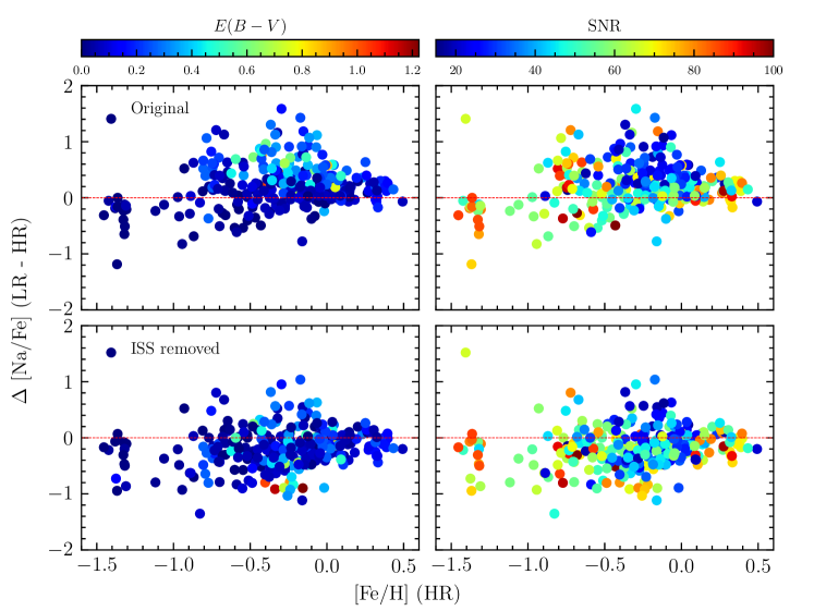
Figure 4.— Same as in Figure 3, but for comparison with APOGEE. The color bar at the top left is added and represents the 3D reddening value derived from Green et al. (2019) after adopting $Gaia$ parallaxes. There are 299 stars included.

2.3. Method for Determination of [Na/Fe]

In order to estimate [Na/Fe] from SDSS stellar spectra with the ISS lines removed, we applied a similar spectral-matching technique as that currently used in the SSPP (Lee et al., 2011, 2013). Briefly, we first generated a grid of synthetic spectra with wide ranges of stellar parameters and [Na/Fe] values. We employed the Kurucz NEWODF model atmospheres (Castelli & Kurucz, 2003), which assumes plane-parallel line-blanketed model structures in one-dimensional local thermodynamical equilibrium (LTE). Then, we utilized the TURBOSPECTRUM synthesis code (Alvarez & Plez, 1998), which adopts the solar abundances of Asplund et al. (2005), to create a synthetic spectrum in the wavelength range between 5500 Å and 6500 Å at a resolving power of $R$ = 500,000. The generated grid covers 4000 K $\leq T_{\rm{eff}}\leq$ 7000 K in steps of 250 K, $0.0\leq$ log $g$ $\leq 5.0$ in steps of 0.5 dex, –5.0 $\leq$ [Fe/H] $\leq$ +1.0 in steps of 0.5 dex, and –1.0 $\leq$ [Na/Fe] $\leq$ +3.0 in steps of 0.5 dex. A total of 16,731 synthetic spectra were generated. Then, these spectra were degraded to the SDSS resolution ($R$ = 2000) and normalized with a pseudo continuum, which was derived from iterative polynomial fitting to a spectrum.

After the radial-velocity correction is made for an observed spectrum, we applied the same continuum routine used for the synthetic grid to the observed SDSS spectrum to obtain a normalized spectrum. From the normalized spectrum, we removed the ISS lines following the methodology described in Section 2.2. The best-matching model spectrum was searched for by minimizing the residuals in the wavelength range of 5880 Å – 5910 Å between the normalized observed spectrum and the synthetic template, using the IDL/MPFIT routine (Markwardt, 2009). The spectral range considered is sufficiently wide to define an accurate continuum and include the Na I D lines. During the minimization, we held $T_{\rm{eff}}$, log $g$, and [Fe/H] constant, and only varied [Na/Fe] to search for the best-fit model. The stellar parameters come from the latest version of the SSPP.

Table 1Systematic and Random Errors of [Na/Fe] due to Errors in Stellar Parameters

	$T_{\rm{eff}}$	$\Delta$[Na/Fe]		log $g$	$\Delta$[Na/Fe]		[Fe/H]	$\Delta$[Na/Fe]
	Error	$\mu$	$\sigma$	Error	$\mu$	$\sigma$	Error	$\mu$	$\sigma$
Type	(K)	(dex)	(dex)	(dex)	(dex)	(dex)	(dex)	(dex)	(dex)
Giant	+100	+0.161	0.035	+0.2	$-$0.023	0.047	+0.2	$-$0.210	0.037
Cool dwarf	+100	+0.155	0.035	+0.2	$-$0.055	0.093	+0.2	$-$0.182	0.041
Hot dwarf	+100	+0.106	0.019	+0.2	$-$0.083	0.119	+0.2	$-$0.190	0.019
Giant	$-$100	$-$0.164	0.039	$-$0.2	+0.017	0.023	$-$0.2	+0.201	0.041
Cool dwarf	$-$100	$-$0.156	0.040	$-$0.2	+0.093	0.047	$-$0.2	+0.183	0.041
Hot dwarf	$-$100	$-$0.107	0.016	$-$0.2	+0.097	0.023	$-$0.2	+0.188	0.024

2.4. Evaluation of the Interstellar Sodium Line-removal Scheme with High-resolution Spectra

2.4.1 Comparison with [Na/Fe] Derived from Gemini/GRACE Stellar Spectra

As part of a study of the early chemical evolution of the MW, we have obtained high-resolution Gemini/GRACES spectra for several dozen extremely metal-poor (EMP; [Fe/H] $<$ –3.0) candidates selected from SDSS and LAMOST, and analyzed these spectra with MOOG (Sneden, 1973) to derive stellar parameters and abundances for various chemical elements, including Na (M. Jeong et al. in preparation). Eleven of the EMP candidates have [Na/Fe] $>$ –0.5, and we make use of them to evaluate the performance of our ISS line-removal scheme by comparing our [Na/Fe] estimates from the low-resolution spectra before and after removing the ISS lines with those of the high-resolution analysis.

To remove the ISS lines from the Gemini/GRACES spectra in a similar fashion as we do for observed SDSS stars, we first measured their EWs in the original high-resolution spectrum, and derived the two Gaussian line profiles following the method described in Section 2.2. These derived line profiles were convolved to the SDSS resolution and subtracted from the degraded high-resolution spectrum. Following this step, we determined [Na/Fe] via our spectral-fitting technique. While determining [Na/Fe], we fixed the stellar parameters adopted from the high-resolution analysis. We also determined [Na/Fe] from the degraded high-resolution spectrum including the ISS lines.

Figure 3 shows the results of this exercise. The color bar shown above the top panel represents the SNRs of the high-resolution spectra. The upper panel shows the difference in the derived [Na/Fe] between our low-resolution estimate and that of the high-resolution analysis before the ISS line removal. It is apparent that the ISS lines overwhelm the intrinsic stellar Na I D lines, resulting in an estimated [Na/Fe] that is systematically higher compared to the high-resolution spectra, by over 1 dex. In the lower panel, which applies to the situation after the removal of the ISS lines, there is a much smaller offset (less than 0.5 dex for most of the stars). Although we did not find any trend with SNR, our estimate of [Na/Fe] is slightly larger, on average, by about 0.2 dex.

We also found that the EWs computed from the ISS lines in the high-resolution spectra are actually quite close to those predicted from the relations between the reddening and EWs of the ISS lines described above. The sum of EWs of the doublets calculated from the 3D extinction map is on average about 6% larger than that measured for the high-resolution spectrum. This result shows that our method for ISS line removal works quite well.

2.4.2 Comparison with [Na/Fe] Derived from APOGEE

We also carried out a similar set of evaluations using data from APOGEE. The APOGEE survey obtains H-band spectra with a resolving power of $R\sim$ 22,500. Even though the APOGEE Data Release 16 (DR16; Ahumada et al., 2020) lists [Na/Fe] abundances determined from different Na lines (16378 Å and 16393 Å), this test still provides a valuable comparison. Note that the Na abundance we adopted from APOGEE is based on the LTE assumption.

Figure 4 shows the difference between the APOGEE results and our measured [Na/Fe] from the Na I D lines with (top panels) and without (bottom panels) the ISS lines, similar to Figure 3. From inspection, it is obvious that our estimated [Na/Fe] is consistently higher in the top panels, in particular for the stars with the higher reddening, as expected. We also note from inspection of the bottom-left panel that our ISS removal scheme has a tendency to slightly over-estimate the EW of the ISS for high-reddening stars, as they exhibit lower [Na/Fe], on average. This behavior is opposite to that seen in Figure 3, where we removed the predicted ISS lines from the high-resolution spectrum. For our present investigation (comparison of field stars with MW GCs, as described below), we are more interested in stars with [Fe/H] $>$ –2.5; thus we rely on the comparison with the APOGEE for further calibration (see Section 3.4). We note that no significant trends with [Fe/H] or SNR are apparent in the right-column panels.

Table 2Impacts of SNR for Low-Resolution Spectra on Determination of [Na/Fe]

	$\Delta$[Na/Fe]
	Giant		Cool dwarf		Hot dwarf
SNR	$\mu$	$\sigma$	$\mu$	$\sigma$	$\mu$	$\sigma$
10	0.022	0.036	0.039	0.049	0.076	0.075
15	0.006	0.029	0.013	0.036	0.034	0.058
20	$-$0.002	0.025	0.002	0.030	0.017	0.054
30	$-$0.009	0.020	$-$0.003	0.026	$-$0.000	0.038
40	$-$0.011	0.017	$-$0.006	0.020	$-$0.006	0.031
50	$-$0.012	0.017	$-$0.005	0.019	$-$0.010	0.027

3. Validation of [Na/Fe] Determinations from Low-Resolution Spectra

3.1. Random and Systematic Errors on [Na/Fe]

The strength of the Na I D lines increases at higher [Fe/H] and [Na/Fe], as expected, and are weaker for giants compared to dwarfs. Thus, a degeneracy could exist in the strength of the Na I D lines depending on stellar parameters, which could result in a systematic error in the estimated [Na/Fe] by our spectral-fitting method. In addition, as we fixed $T_{\rm eff}$, $\log~{}g$, and [Fe/H] while estimating [Na/Fe], the existence of any systematic errors in $T_{\rm eff}$, $\log~{}g$, and [Fe/H] could produce a systematic error in the determined [Na/Fe]. Therefore, we need to check how the systematic errors in the adopted stellar parameters and the possible degeneracy of the Na I D line strengths affects the estimated [Na/Fe].

To carry out this test, we first processed the synthetic spectra through our methods to obtain an estimate of the (known) [Na/Fe] under various conditions. While estimating [Na/Fe], we shifted the model parameters by $\pm$100 K for $T_{\rm{eff}}$ and $\pm$0.2 dex for log $g$ and [Fe/H], respectively, in order to estimate how much the derived [Na/Fe] can be affected by errors of the adopted stellar parameters.

After completing the estimates of [Na/Fe] to check the collective behavior of the determined [Na/Fe], we divided the measured [Na/Fe] values into three groups: giants for $T_{\rm eff}$ $<$ 5500 K and $\log~{}g$ $<$ 3.5, cool dwarfs for $T_{\rm eff}$ $<$ 5500 K and $\log~{}g$ $\geq$ 3.5, and hot dwarfs for $T_{\rm eff}$ $\geq$ 5500 K and $\log~{}g$ $\geq$ 3.5. We did not include the spectra for models with [Fe/H] $<$ –3.0, because not only are such objects rare, but we are here primarily interested in the escaped stars from the Galactic GCs or the debris from the already-disrupted GCs, which presumably have [Fe/H] $>$ –3.0.

Table 1 summarizes the results of the above exercise. It generally indicates that the systematic offsets of the measured [Na/Fe] do no vary much among the different groups, and that the random scatters are also small for all groups. Specifically, the incorrect assignment of surface gravity does not much affect the measured [Na/Fe], as the mean offset is less than 0.1 dex. The errors caused by the $T_{\rm eff}$ and [Fe/H] offsets become a little larger, up to $\pm$0.16 dex and $\pm$0.2 dex, respectively, but are still not significant. The mean $\mu$ and standard deviation $\sigma$ in the table are determined from a Gaussian fit to the differences between our estimates and the model values. Considering that the typical uncertainty of the elemental abundance from the low-resolution spectroscopy is about 0.3 dex, we conclude that the systematic errors in the stellar parameters do not significantly affect the estimated [Na/Fe].

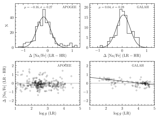
Figure 5.— Comparison of our derived sodium-abundance ratios with those from the APOGEE (left panels) and GALAH (right panels) surveys, which are based on high-resolution near-IR and optical spectroscopy, respectively. In the upper panels, the mean offset ($\mu$) and the standard deviation ($\sigma$) were obtained by fitting a Gaussian to both samples. The comparison with the APOGEE data exhibit no significant trend with $\log~{}g$, so we decided to adjust the offset (–0.16 dex) to the [Na/Fe] value before applying the NLTE corrections described in the text (see Section 3.3. Since [Na/Fe] from the GALAH survey is based on NLTE, we compared our values of [Na/Fe] after the NLTE correction to those from the GALAH stars. The top-right panel indicates a small offset (less than 0.1 dex). However, we note a negative trend with surface gravity in the bottom-right panel. We fitted a linear function to the residuals to obtain a slope of –0.21 dex dex^-1 and intercept of 0.88 dex. We applied this correction function to our NLTE corrected [Na/Fe], and use this value for further analysis.

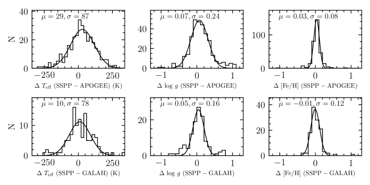
Figure 6.— Comparison of the stellar parameters from the SSPP with those from the APOGEE (upper panels) and GALAH (lower panels) data based on high-resolution spectroscopic analysis. The mean offset and the scatter for each parameter are derived from a Gaussian fit. Overall, we observe relatively small offsets and scatters from both samples for all three parameters. This figure only includes the stars with [Na/Fe] available in the APOGEE and GALAH data sets, as we calibrate our estimates of [Na/Fe] with those from these two surveys. Note that we used the NLTE [Fe/H] values from the GALAH survey; see the text for details on the validity of its use.

3.2. Impact of SNR on Estimated [Na/Fe]

Stellar spectra from large sky surveys such as SDSS and LAMOST cover a wide range of SNRs. Because the noise in a spectrum is able to induce systematic and random errors, we also check on how the SNR affects the estimated [Na/Fe].

To evaluate the impact of the SNR on the abundance estimate for sodium, following Lee et al. (2008a), we injected different levels of random noise into the grid of synthetic spectra used for the spectral fitting. In this process, we generated a set of 10 different noise-added synthetic spectra for SNR = 10, 15, 20, 30, 40, and 50 per given model spectrum. Then, we applied our method to the noise-added synthetic spectra to recover [Na/Fe]. In our analysis, we took an average value of 10 [Na/Fe] values from 10 simulated noise-injected spectra at a given SNR. To analyze the results of this test, once again we divided the test sample into three groups as in Section 3.1: giants, cool dwarfs, and hot dwarfs.

Table 2 summarizes the results of the above exercise. It indicates that, even though there is a tendency that the mean offset and scatter increase with decreasing SNR, as expected, their size is relatively small. The mean $\mu$ and standard deviation $\sigma$ in the table are determined from a Gaussian fit to the residuals between our estimates and the model parameters for [Fe/H]$\geq$ –3.0. Furthermore, we observe that, as the metallicity decrease and temperature increases, the mean difference and their scatter become larger, presumably due to the weaker Na I D lines. Nonetheless, the mean offset and scatter are significantly less than 0.1 dex for all three groups and SNRs. Consequently, this exercise confirms that our method is very robust to the SNR of the spectrum.

3.3. Non-LTE Corrections

It is known that the [Na/Fe] abundance ratio can vary, by as much as 0.5 dex, under the non-LTE (NLTE) assumption, especially when the EW of the Na I D lines is around 150 to 200 mÅ (Gratton et al., 1999; Lind et al., 2011). The correction is generally larger for giants than dwarfs (Amarsi et al., 2020). Therefore, we need to apply NLTE corrections to our measured [Na/Fe]. Gratton et al. (1999) reported the NLTE corrections for lines of Fe I, O I, Na I, and Mg I, and provided the correction values for stars with $T_{\rm eff}$ from 4000 K to 7000 K with 1000 K steps, over a broad range of gravities ($\log~{}g$ = 1.5, 3.0, 4.5) and metallicities ([Fe/H] = 0, –1, –2, –3). For the Na I D lines the correction grid is valid for the EW range of 100 mÅ – 1350 mÅ. We adopted this grid to derive the NLTE correction value by linear interpolation over the stellar parameters and the EW of the Na I D lines. When obtaining the correction value from this interpolation, we used the EW of the Na I D lines calculated from the synthetic spectrum, which is generated with the estimated $T_{\rm eff}$, $\log~{}g$, [Fe/H], and [Na/Fe] for each star, because it provides much clearer lines to calculate the EW. We simply took the value from the grid that is the nearest to $T_{\rm eff}$, $\log~{}g$, [Na/Fe], and EW for the star whose parameters are outside the grid.

3.4. Calibration of Estimated [Na/Fe] with High-resolution Surveys

Comparison of our derived [Na/Fe] with that estimated based on high-resolution spectroscopy provides a direct measure of the reliability of our estimated [Na/Fe]. We employed stars observed in two surveys, APOGEE and the Galactic Archaeology with HERMES (GALAH; Zucker et al., 2012) survey. The GALAH survey obtained optical spectra with a resolving power of $R\sim$ 28,000. Although the APOGEE DR16 and the GALAH Data Release 3 (Buder et al., 2021) contain [Na/Fe] abundances determined from different Na lines: 16378 Å and 16393 Å for APOGEE and 5688 Å, 6154 Å, and 6169 Å for GALAH, we expect the derived Na abundance ratio should be the same independent of the lines employed, unless some unexpected problem exists. Below we describe a comparison exercise between the two surveys.

Cross matches (within 1$\arcsec$) were used to identify 318 and 116 stars in common between SDSS and APOGEE, and SDSS and GALAH, respectively. We selected only the stars with $T_{\rm eff}$ = 4000 – 7000 K and the uncertainties of the measured [Na/Fe] less than 0.1 dex in the comparison-survey data. These stars also met the requirement of 10 km s^-1 in radial-velocity differences. For the SDSS spectra, we removed the ISS lines following the scheme described in Section 2.2. We adopted for each star the inverse parallax from $Gaia$ EDR3 as the distance used to calculate the strength of the ISS lines. The sodium-abundance ratio was then determined by fixing the atmospheric parameters ($T_{\rm eff}$, $\log~{}g$, and [Fe/H]) obtained from the SSPP.

Note that the [Na/Fe] abundance ratio from APOGEE is based on an LTE assumption, while that from the GALAH is based on the NLTE assumption. To carry out the calibration properly, we first compared our measured value before the NLTE correction with that of APOGEE to check if any systematic error exists in the LTE value. The left column of panels in Figure 5 show histograms of the [Na/Fe] differences (top panel) between our low-resolution (LR) and the APOGEE high-resolution (HR) value, and their trend with $\log~{}g$ (bottom panel). We found a systematic offset of –0.16 dex and a standard deviation of 0.27 dex, which were calculated with a Gaussian fit to the residuals. The bottom panel suggests no significant trend of the mean offset with $\log~{}g$. From these findings, we decided to adjust our estimated LR LTE [Na/Fe] by 0.16 dex to place it on the same abundance scale as for the HR LTE APOGEE sample.

To compare with the GALAH data, after the 0.16 dex offset described above is applied to our LR LTE estimates, we corrected them to the NLTE scale following the recipe described in Section 3.3. The Na abundance differences with respect to GALAH and their trend with $\log~{}g$ are displayed in the right column of panels shown in Figure 5. Our LR NLTE Na abundances exhibit a very small systematic offset of 0.04 dex, as shown in the top panel. The lower panel, however, indicates a negative trend with $\log~{}g$. In order to eliminate this trend, we used a linear fit, with slope and intercept of –0.21 dex dex^-1 and 0.88 dex, respectively, and applied it to our LR NLTE values. We noticed no significant trend with $T_{\rm eff}$ or [Fe/H] after this correction was applied.

To summarize our approach for determination of the final adopted [Na/Fe] estimates, we first add 0.16 dex to our measured LR [Na/Fe], obtain the NLTE-corrected value, and apply the correction function found in the bottom-right panel of Figure 5 to determine the final LR NLTE [Na/Fe] estimate. We use this final value for the following analysis. The comparisons with the high-resolution data and the other two tests described in Sections 3.1 and 3.2 suggest that the expected precision of the estimated [Na/Fe] is better than 0.3 dex for [Fe/H] $>$ –2.0 and SNR $>$ 10.

3.5. Accuracy of the Stellar Parameters Determined by the SSPP

We also compared the stellar parameters delivered by the SSPP to those from the APOGEE and GALAH surveys to check their accuracy and uncertainties, because any systematic error in the SSPP stellar parameters can result in systematic deviations in the determined [Na/Fe], as demonstrated in Section 3.1. Note that we employed the SDSS stars in common with stars from the APOGEE and GALAH surveys with [Na/Fe] available, as we used them to calibrate our estimates of [Na/Fe]. Figure 6 shows the distributions of the differences in $T_{\rm eff}$ (left), $\log~{}g$ (middle), and [Fe/H] (right) for the APOGEE (upper panels) and GALAH (lower panels) data. The mean difference ($\mu$) and the standard deviation ($\sigma$) are derived from a Gaussian fit to each distribution. We note the very small mean offsets and scatters for both surveys. Specifically, the temperature comparison indicates that the zero-point offset is less than 30 K, with a scatter less than 90 K. The gravity comparison shows $\mu<$ 0.1 dex with $\sigma<$ 0.25 dex, and $\mu<$ 0.05 dex with $\sigma<$ 0.15 dex for the metallicity. Note that the metallicity from the GALAH survey is the NLTE value. As the NLTE correction for [Fe/H] is very small (mostly less than 0.1 dex) for the stars with [Fe/H] $>$ –1.0 (Lind et al., 2012) and most of the GALAH stars have [Fe/H] $>$ –1.0, we simply used the NLTE value of [Fe/H] for this comparison.

Taking into account that the SDSS stellar spectrum is low resolution, these mean offsets and scatters are quite small, suggesting that the SSPP recovers estimates of the stellar parameters very well.

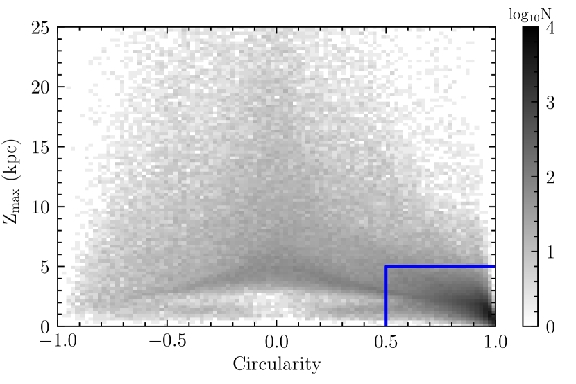
Figure 7.— Density map of our sample stars in $Z_{\rm{max}}$ versus circularity space. Positive and negative circularity values correspond to prograde and retrograde motions, respectively. The stars inside the blue box are regarded to be of $in\,situ$ origin, while the objects outside the box are taken to be of accreted origin. Note that, although a number of stars with $r_{\rm{max}}<3.5$ kpc are located outside the blue box, they are regarded as belonging to the $in~{}situ$ origin (see text).

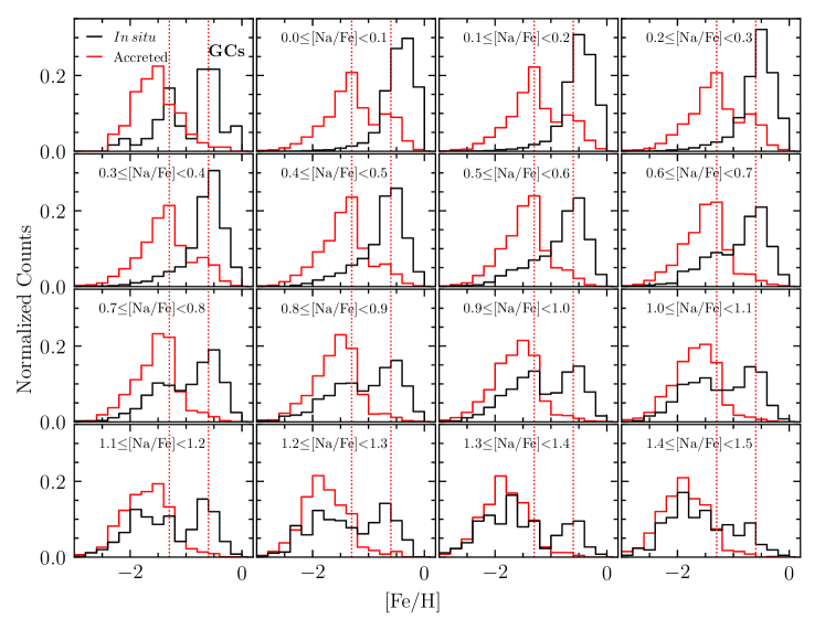
Figure 8.— Metallicity distribution functions (MDFs) of the $in\,situ$ (black) and the accreted (red) components, which are grouped by the dividing scheme of Massari et al. (2019). The histogram is normalized by the total number of stars in each group. The top-left panel shows the MDFs of the GCs. The $in~{}situ$ GCs display two peaks around [Fe/H] = –1.3 and –0.6, respectively, whereas the accreted component exhibits one peak at [Fe/H] = –1.6. The two vertical dotted reference lines are provided at [Fe/H] = –1.3 and –0.6, respectively. The other panels present the MDFs of our sample of stars in different ranges of [Na/Fe]. Notice the rise of the second peak in the $in~{}situ$ sample from [Na/Fe] = +0.6; as the Na-abundance ratio increases, the portion of the metal-poor stars increases as well. In comparison, the accreted population displays two peaks at low [Na/Fe], and they disappear above [Na/Fe] $\sim$ +0.5; its MDF is gradually shifted to the low-metallicity regime with increasing [Na/Fe].

4. An Example Application

Here we describe an example application of our sodium-abundance ratio estimates for a large sample of stars with available low-resolution spectra from SDSS. Other applications are clearly of interest, which we will pursue in future papers. When the currently observed GCs in the MW are divided into the $in~{}situ$ and accreted component by their dynamical properties (e.g., Massari et al., 2019), their MDFs are dissimilar, with distinct characteristics. As the Na-rich stars are believed to have originated from stripped or totally disrupted GCs, we might expect that their dynamical properties and chemical characteristics may be similar to those observed in the surviving GCs, but different for the Na-normal stars. We explore this hypothesis below.

4.1. The Field Star Sample

We applied our method for determining [Na/Fe] to 539,920 stellar spectra with SNR $\geq$ 10, which were assembled from the SDSS stars. We adopted parallaxes from $Gaia$ EDR3 to calculate the distances, which we require to estimate the strength of the ISS lines from the 3D reddening map. When calculating the distance, we corrected the global parallax offset of $+$0.017 mas (Lindegren et al., 2021). After the corrections for NLTE effects and the systematic offset described in Sections 3.3 and 3.4, respectively, we are left with a total number of 427,799 stars with available LR NLTE [Na/Fe] values.

4.2. Calculation of Space Velocities and Orbital Parameters

For the dynamical study of our program stars we require information on their velocity components and orbital parameters. We employed the proper motions and parallaxes from $Gaia$ EDR3 and the radial velocities from the SDSS spectra, and computed the $U,V,W$ velocity components and dynamical parameters, including the maximum ($r_{\rm max}$) and minimum ($r_{\rm min}$) distances from the Galactic center, maximum distance ($Z_{\rm max}$) from the Galactic plane, orbital eccentricity ($e$), angular momentum, and energy, etc., using the galpy Python package (Bovy, 2015), adopting the Galactic gravitational potential model of McMillan (2017). During these calculations, we integrated the orbit of each star over 13 Gyr with 1 Myr steps, and assumed $V_{\rm{LSR}}$ = 233.1 km s^-1 for the Local Standard of Rest, a solar peculiar motion of ($U,V,W$)_⊙ = (11.1, 12.24, 7.25) km s^-1 (Schönrich et al., 2010), and the distance of the Sun from the Galactic center of $R_{\odot}$ = 8.21 kpc. The orbital parameters of Galactic GCs were also computed by adopting their positions, proper motions, distances, and radial velocities from Vasiliev (2019).

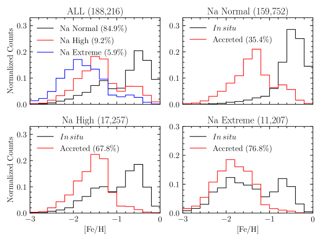
Figure 9.— Metallicity distribution functions (MDFs) of our sample according to their level of Na enhancement: all (upper left), [Na/Fe] $<$ +0.6 (upper right), +0.6 $\leq$ [Na/Fe] $<$ +1.0 (lower left), and [Na/Fe] $\geq$ +1.0 (lower right). It is clear to see in the upper-left panel that all three subgroups have different peaks and shapes of their MDFs. About 85 % of our sample stars belong to the Na-normal subgroup, and only 15 % of stars have [Na/Fe] $\geq+0.6$. The other panels show the MDFs of the $in\,situ$ and accreted stars for the three subgroups. The fraction of the accreted stars clearly increases with increasing [Na/Fe].

4.3. Results and Discussion

Among the SDSS stars with estimated [Na/Fe] and available orbital parameters, we selected the stars with 4400 K $\leq$ $T_{\rm{eff}}$ $\leq$ 7000 K, –3 $\leq$ [Fe/H] $\leq 0$, and SNR $\geq$ 25.0 to ensure the most reliable measurement of [Na/Fe]. We also imposed on our sample stars the requirement of the renormalized unit weight error less than 1.4 from $Gaia$ EDR3 to select stars with good astrometric solutions. For stars with derived $r_{\rm max}$ $\leq$ 200 kpc, we ended up with a final sample of 188,216 stars.

Provided that the Na-rich stars originated from GCs or disrupted GCs, we may expect that their MDF and dynamical properties would be similar to those of the GCs. In addition, they would exhibit distinct features in their MDF, compared to those from the Na-normal stars. To identify their connection to the GCs, we followed a similar approach as Massari et al. (2019). They divided the GCs into $in\,situ$ (bulge and disk clusters) and accreted clusters, using their dynamical properties. They defined that the bulge clusters have small orbits with $r_{\rm max}$ $<3.5$ kpc, and disk clusters have orbital circularity larger than 0.5 and $Z_{\rm{max}}<5$ kpc. Note that the orbital circularity is defined as $L_{Z}/L_{Z,\rm{circ}}$, where $L_{Z,\rm{circ}}$ is the angular momentum of a circular orbit with a cluster’s energy. Figure 7 displays the density map of our sample stars on $Z_{\rm{max}}$ versus circularity space. In the figure, positive and negative circularity values mean prograde and retrograde orbits, respectively. The stars inside the blue box are classified as of the $in\,situ$ origin, while outside the box they are considered of accretion origin.

After dividing into the two groups, we first inspected the MDFs of each group in different bins of [Na/Fe] values, as shown in Figure 8. The top-left panel of the figure shows the MDFs of the GCs in the MW. The black histogram is for the $in\,situ$ GCs, while the red histogram is for the accreted GCs, divided by following the work by Massari et al. (2019). The [Fe/H] values of the GCs were adopted from the Harris (1996, 2010) catalog. The notable features in this panel are that the MDF of the accreted GCs has only a single peak at [Fe/H] $\sim$ –1.6, with more objects populating the more metal-poor region, while the MDF of the $in\,situ$ GCs exhibits two peaks at [Fe/H] = –1.3 and –0.6, respectively, indicated by the two vertical dotted lines. The rest of the panels in the figure show the MDFs of our program stars.

Inspection of the MDFs in each panel reveals that the MDF for the $in~{}situ$ population of stars peaks at between [Fe/H] = –0.6 and –0.4, with a long tail toward the low-metallicity region, up to [Na/Fe] = +0.6. These Na-normal, metal-rich stars are the dominant sources of the canonical Thick Disk (TD) and Metal-Weak Thick Disk (MWTD; Carollo et al., 2019). The second peak at [Fe/H] = –1.3 starts to rise from [Na/Fe] = +0.6, and the first peak remains the same, at [Fe/H] = –0.6, for [Na/Fe] $>$ +0.6. These features qualitatively agree with those of the $in~{}situ$ GCs, as can be seen in the top-left panel. From [Na/Fe] = +1.0 to [Na/Fe] = +1.5, the second peak becomes more obvious, with a much broader, but more metal-poor, distribution, while the fist peak still exists. The much larger scatter and more metal-poor feature in the second peak may imply that more than one population contributes to the second peak. Even though they are defined as the $in~{}situ$ component, it is possible that some of the metal-poor component came from the accreted GCs, as claimed by Woody & Schlaufman (2021), who argue that the metal-poor GCs are mostly accreted from disrupted dwarf galaxies.

The accreted population of our sample fairly well follows the shape of the MDF of the accreted GCs above [Na/Fe] = +0.5. For [Na/Fe] $<$ +0.5, we can also observe a second peak at [Fe/H] = –0.6. Considering their metallicity and distinct dynamical status, this group of stars may consist of the GE (Helmi et al., 2018) and Splashed Disk (SD; Belokurov et al., 2020), and the rest of the more metal-poor stars may contribute to the Sequioa (Myeong et al., 2019) and Thamnos 1 & 2 (Koppelman et al., 2019) structures. We note in Figure 8 that the low-metallicty tails of the MDFs of the $in~{}situ$ and the accreted populations in the range of [Na/Fe] $>$ +0.9 exhibit similar peaks and shapes. This analogy may suggest that the low-metallicity, Na-rich stars may share chemically similar GC progenitors.

For the ensemble view of the $in~{}situ$ and the accreted populations of our sample, based on the MDF characteristics found in Figure 8, we divided our sample into three subgroups: Na-normal stars with [Na/Fe]$<$ +0.6, Na-high stars with +0.6 $\leq$ [Na/Fe] $<$ +1.0, and Na-extreme stars with [Na/Fe] $\geq$ +1.0, and explored differences in their MDFs, as shown in Figure 9.

The upper-left panel of Figure 9 displays the MDFs of the three subgroups, normalized by the total number of stars in each subgroup. Different peaks and morphologies for the MDFs are evident. The general behavior is that the higher the sodium-abundance ratio, the lower the metallicity peak. About 85% of our sample stars belong to the Na-normal subgroup, and only 15% of stars have [Na/Fe] $\geq$ +0.6. The other three panels exhibit the MDFs of the $in\,situ$ (black) and accreted (red) stars for each subgroup. The $in\,situ$ stars of the Na-normal subgroup (upper right) exhibits a single peak at [Fe/H] $\sim$ –0.5 with a long metal-poor wing. This group of stars comprises mainly the canonical TD and MWTD. On the other hand, the accreted subgroup displays a single peak at [Fe/H] $\sim$ –1.3, without much skewness. This subgroup comprises the GS, GE, and SD stars. The two MDFs are reminiscent of the local disk and halo populations in the MW.

About 9.2% of stars (lower-left panel of Figure 9) among our sample belong to the Na-high subgroup. The shapes of the MDFs of the $in\,situ$ and accreted stars in this subgroup are very similar to those of the GCs (see the upper-left panel of Figure 8) — a single peak around [Fe/H] = –1.6 for the accreted population and the double peaks around [Fe/H] = –1.3 and –0.6 for the $in\,situ$ population. As Galactic field stars mostly have [Na/Fe] $<$ +0.5 (Suda et al., 2008), and the Na-high stars have the same characteristics in their MDF as the Galactic GCs, we can confirm that the stars in the Na-high subgroup are likely the escaped stars from present GCs.

The MDFs of the Na-extreme subgroup (lower-right panel of Figure 9) present some distinct features compared to the Na-normal and Na-high subgroups. Although the $in~{}situ$ population still has two peaks, the metal-poor stars are more prominent. The accreted component is also more metal-poor and has a broader distribution. One notable feature is that the metal-poor component ([Fe/H] $<$ –1.2) of the MDF for the $in~{}situ$ population generally follows that of the accreted component, a characteristic that does not appear for the surviving GCs. Consequently, it is plausible that the metal-poor stars in the Na-extreme subgroup may have originated from already disrupted metal-poor GCs, and experienced similar chemical evolution, but different dynamical evolution. Another possible interpretation is that the $in~{}situ$ metal-poor stars may not be the stars formed in $in~{}situ$ GCs. According to the analysis of Piatti (2019), among the prograde GCs, which are assumed to be of the $in~{}situ$ origin, the number of accreted GCs is similar to that of the $in~{}situ$ ones. Following this reasoning, some of the stars in our metal-poor, Na-extreme $in~{}situ$ population may originate from accreted GCs. This interpretation is in line with the claim by Woody & Schlaufman (2021).

Regarding the metal-rich ([Fe/H] $>$ –1.0) $in~{}situ$ population in the Na-high and Na-extreme subgroups, we note that these may be related to the metal-rich ([Fe/H] $>$ –0.7) population recently discovered from APOGEE data by Fernández-Trincado et al. (2021). These authors claimed that this population is likely to be stellar debris from partially or fully disrupted metal-rich GCs.

Another point to consider is that some fraction of Carbon-Enhanced Metal-Poor (CEMP; Beers & Christlieb, 2005) stars exhibit enhancements of sodium although many of the CEMP stars exhibit [Na/Fe] $<$ 0.5 (Spite et al., 2014; Hansen et al., 2015; Yoon et al., 2016; Purandardas & Goswami, 2021). Thus, our Na-extreme stars may also be related to CEMP stars. Indeed, when we considered as CEMP stars the objects with [Fe/H] $<$ –1.0 and [C/Fe] $>$ +0.7, we found from the Na-extreme subgroup that the fraction of CEMP stars for [Fe/H] $<$ –1.0 is 12.0%; it increases to 18.7% for [Fe/H] $<$ –2.0. This proportion is much higher than those of previous studies (e.g., Lee et al., 2013). We also found that the CEMP fraction (19.1%) of the accreted component in the Na-extreme subgroup is higher than that (16.3%) of the $in~{}situ$ component for [Fe/H] $<$ –2.0. In the metallicity range of [Fe/H] $>$ –2.5, the CEMP-$s$ (those enhanced with slow neutron-capture elements) stars are dominant among the different CEMP subclasses (Aoki et al. 2007; see also Yoon et al. 2016, 2018); hence their likely progenitors are asymptotic giant branch (AGB) stars. Furthermore, the second-generation stars observed in GCs exhibit low carbon and high nitrogen abundances. These results suggest that many of the Na-extreme stars probably did not originate from GCs.

Taking into account only the Na-high stars, we obtained the fraction of 9.2% (17257/188216), which is within the fractions reported by previous studies (Carretta et al., 2010; Martell et al., 2011; Ramírez et al., 2012). This fraction implies a non-negligible contribution from the GCs to the build-up of the Galactic halo.

To sum up, since the $in~{}situ$ and accreted stars of our Na-high stars exhibit similar MDFs to those of present GCs, they may have originated from these, but this is not the case for the Na-extreme stars. As the fraction of the Na-high stars is 9.2%, the contribution from GC-origin stars to the build-up of the Galactic halo appears non-negligible. Furthermore, because the metal-poor stars in the $in~{}situ$ and accreted populations exhibit similar MDFs, we cannot rule out that they may share the progenitors with similar chemical-evolution histories. Indeed, a K-S two-sample test between MDFs for the $in~{}situ$ and accreted stars with [Fe/H] $<$ –1.2 in the Na-extreme subgroup yielded a $p$-value of 0.0722, which is small, but only permits a marginal rejection of their selection from the same parent population.

5. Summary

We have presented a method for the estimation of [Na/Fe] from low-resolution stellar spectra. To determine [Na/Fe] more accurately, we developed a technique of removing the ISS lines in a stellar spectrum, using the correlation between the Galactic reddening, $E(B-V)$, and the strength of Na I D doublet lines produced by the ISM. In addition, we applied an NLTE correction to determine [Na/Fe] more accurately and precisely. We also investigated the MDFs of the Na-rich stars, and compare with those of Galactic GCs, in order to better understand the connection of the Na-rich stars with the buildup of the Galactic halo. In a subsequent paper, we will carry out a more thorough analysis of the Na-rich stars gathered from SDSS and LAMOST, using their chemical and dynamical properties to unravel their relation to the GCs and the Galactic halo assembly.

We also note that our measured [Na/Fe] will be extremely useful to calibrate photometrically estimated [Na/Fe] for stars from narrow-band photometric surveys such as Javalambre Photometric Local Universe Survey (J-PLUS; Cenarro et al., 2019) and the Southern Photometric Local Universe Survey (S-PLUS; Mendes de Oliveira et al., 2019). Eventually, these efforts should result in tens to hundreds of million stars with measured [Na/Fe] to explore various stellar populations in the MW.

References

- Ahumada et al. (2020) Ahumada, R., Prieto, C. A., Almeida, A., et al. 2020, ApJS, 249, 3
- Allende Prieto et al. (2008) Allende Prieto, C., Sivarani, T., Beers, T. C., et al. 2008, AJ, 136, 2070
- Alvarez & Plez (1998) Alvarez, R. & Plez, B. 1998, A&A, 330, 1109
- Amarsi et al. (2020) Amarsi, A. M., Lind, K., Osorio, Y., et al. 2020, A&A, 642, 62
- Aoki et al. (2007) Aoki, W., Beers, T. C., Christilieb, N., et al. 2007, ApJ, 655, 492
- Asplund et al. (2005) Asplund, M., Grevesse, N., & Sauval, A. J. 2005, Cosmic Abundances as Records of Stellar Evolution and Nucleosynthesis, 336, 25
- Beers & Christlieb (2005) Beers, T. C., & Christlieb, N. 2005, ARA&A, 43, 531
- Belokurov et al. (2018) Belokurov, V., Erkal, D., Evans, N. W., et al. 2018, MNRAS, 478, 611
- Belokurov et al. (2020) Belokurov, V., Sanders, J. L., Fattahi, A., et al. 2020, MNRAS, 494, 3880
- Blanton et al. (2017) Blanton, M. R., Bershady, M. A., Abolfathi, B., et al. 2017, AJ, 154, 28
- Bovy (2015) Bovy, J. 2015, ApJS, 216, 29
- Buder et al. (2021) Buder, S., Sharma, S., Kos, J., et al. 2021, MNRAS
- Carollo et al. (2019) Carollo, D., Chiba, M., Ishigaki, M., et al. 2019, ApJ, 887, 22
- Carretta (2016) Carretta, E. 2016, arXiv:1611.04728
- Carretta et al. (2009) Carretta, E., Bragaglia, A., Gratton, R. G., et al. 2009, A&A, 505, 117
- Carretta et al. (2010) Carretta, E., Bragaglia, A., Gratton, R. G., et al. 2010, A&A, 516, A55
- Castelli & Kurucz (2003) Castelli, F. & Kurucz, R. L. 2003, Modelling of Stellar Atmospheres, 210, A20
- Cenarro et al. (2019) Cenarro, A. J., Moles, M., Cristóbal-Hornillos, D., et al. 2019, A&A, 622, A176
- Chene et al. (2014) Chene, A. -N, et al. 2014, GRACES: Gemini remote access to CFHT ESPaDOnS spectrograph through the longest astronomical fiber ever made: experimental phase completed. p. 915147, doi:10.1117/12.2057417
- Cui et al. (2012) Cui, X.-Q., Zhao, Y.-H., Chu, Y.-Q., et al. 2012, Research in Astronomy and Astrophysics, 12, 1197
- D’Antona et al. (2016) D’Antona, F., Vesperini, E., D’Ercole, A., et al. 2016, MNRAS, 458, 2122
- D’Ercole et al. (2010) D’Ercole, A., D’Antona, F., Ventura, P., et al. 2010, MNRAS, 407, 854
- Dawson et al. (2013) Dawson, K. S., Schlegel, D. J., Ahn, C. P., et al. 2013, AJ, 145, 10
- Fernández-Trincado et al. (2016) Fernández-Trincado, J. G., Robin, A. C., Moreno, E., et al. 2016, ApJ, 833, 132
- Fernández-Trincado et al. (2017) Fernández-Trincado, J. G., Zamora, O., García-Hernández, D. A., et al. 2017, ApJ, 846, L2
- Fernández-Trincado et al. (2021) Fernández-Trincado, J. G., Beers, T. C., Queiroz, A. B. A., et al. 2021, ApJ, accepted
- Gaia Collaboration et al. (2016) Gaia Collaboration, Prusti, T., de Bruijne, J. H. J., et al. 2016, A&A, 595, A1
- Gaia Collaboration et al. (2018) Gaia Collaboration, Brown, A. G. A., Vallenari, A., et al. 2018, A&A, 616, A1
- Gaia Collaboration et al. (2021) Gaia Collaboration, Brown, A. G. A., Vallenari, A., et al. 2021, A&A, 649, A1
- Gieles et al. (2018) Gieles, M., Charbonnel, C., Krause, M. G. H., et al. 2018, MNRAS, 478, 2461
- Gratton et al. (1999) Gratton, R. G., Carretta, E., Eriksson, K., et al. 1999, A&A, 350, 955
- Green (2018) Green, G. M. 2018, The Journal of Open Source Software, 3, 695
- Green et al. (2019) Green, G. M., Schlafly, E., Zucker, C., et al. 2019, ApJ, 887, 93
- Hansen et al. (2015) Hansen, T., Hansen, C. J., Christlieb, N., et al. 2015, ApJ, 807, 173
- Harris (1996) Harris, W. E. 1996, AJ, 112, 1487
- Harris (2010) Harris, W. E. 2010, arXiv:1012.3224
- Helmi et al. (2018) Helmi, A., Babusiaux, C., Koppelman, H. H., et al. 2018, Nature, 563, 85
- Horta et al. (2021) Horta, D., Mackereth, J. T., Schiavon, R. P., et al. 2021, MNRAS, 500, 5462
- Ibata et al. (1994) Ibata, R. A., Gilmore, G., & Irwin, M. J. 1994, Nature, 370, 194
- Ito et al. (2013) Ito, H., Aoki, W., Beers, T. C., et al. 2013, ApJ, 773, 33
- Jeong et al. (2021) Jeong, Miji, Lee, Y. S., Kim, Y., Beers, T. C. 2021, in prep
- Koppelman et al. (2019) Koppelman, H. H., Helmi, A., Massari, D., et al. 2019, A&A, 631, L9
- Lee et al. (2011) Lee, Y. S., Beers, T. C., Allende Prieto, C., et al. 2011, AJ, 141, 90
- Lee et al. (2013) Lee, Y. S., Beers, T. C., Masseron, T., et al. 2013, AJ, 146, 132
- Lee et al. (2008a) Lee, Y. S., Beers, T. C., Sivarani, T., et al. 2008a, AJ, 136, 2022
- Lee et al. (2008b) Lee, Y. S., Beers, T. C., Sivarani, T., et al. 2008b, AJ, 136, 2050
- Lee et al. (2019) Lee, Y.-W., Kim, J. J., Johnson, C. I., et al. 2019, ApJ, 878, L2
- Lim et al. (2021) Lim, D., Lee, Y.-W., Koch, A., et al. 2021, ApJ, 907, 47
- Lind et al. (2011) Lind, K., Asplund, M., Barklem, P. S., et al. 2011, A&A, 528, A103
- Lind et al. (2012) Lind, K., Bergemann, M., & Asplund, M. 2012, MNRAS, 427, 50
- Lindegren et al. (2021) Lindegren, L., Klioner, S. A., Hernández, J., et al. 2021, A&A, 649, A2
- Majewski et al. (2017) Majewski, S. R., Schiavon, R. P., Frinchaboy, P. M., et al. 2017, AJ, 154, 94
- Majewski et al. (2003) Majewski, S. R., Skrutskie, M. F., Weinberg, M. D., et al. 2003, ApJ, 599, 1082
- Markwardt (2009) Markwardt, C. B. 2009, Astronomical Data Analysis Software and Systems XVIII, 251
- Martell & Grebel (2010) Martell, S. L. & Grebel, E. K. 2010, A&A, 519, A14
- Martell et al. (2016) Martell, S. L., Shetrone, M. D., Lucatello, S., et al. 2016, ApJ, 825, 146
- Martell et al. (2011) Martell, S. L., Smolinski, J. P., Beers, T. C., et al. 2011, A&A, 534, A136
- McMillan (2017) McMillan, P. J. 2017, MNRAS, 465, 76
- Massari et al. (2019) Massari, D., Koppelman, H. H., & Helmi, A. 2019, A&A, 630, L4
- Mendes de Oliveira et al. (2019) Mendes de Oliveira, C., Ribeiro, T., Schoenell, W., et al. 2019, MNRAS, 1111, 241
- Murga et al. (2015) Mu rga, M., Zhu, G., Ménard, B., et al. 2015, MNRAS, 452, 511
- Myeong et al. (2019) Myeong, G. C., Vasiliev, E., Iorio, G., et al. 2019, MNRAS, 488, 1235
- Pereira et al. (2019) Pereira, C. B., Holanda, N., Drake, N. A., et al. 2019, AJ, 157, 70
- Piatti (2019) Piatti, A. E. 2019, ApJ, 882, 98
- Piatti (2020) Piatti, A. E. 2020, A&A, 643, A77
- Poznanski et al. (2012) Poznanski, D., Prochaska, J. X., & Bloom, J. S. 2012, MNRAS, 426, 1465
- Purandardas & Goswami (2021) Purandardas, M, & Goswami, A. 2021, ApJ, in press, arXiv:2108.06075
- Ramírez et al. (2012) Ramírez, I., Meléndez, J., & Chanamé, J. 2012, ApJ, 757, 164
- Schiavon et al. (2017a) Schiavon, R. P., Johnson, J. A., Frinchaboy, P. M., et al. 2017a, MNRAS, 466, 1010
- Schiavon et al. (2017b) Schiavon, R. P., Zamora, O., Carrera, R., et al. 2017b, MNRAS, 465, 501
- Schlegel et al. (1998) Schlegel, D. J., Finkbeiner, D. P., & Davis, M. 1998, ApJ, 500, 525
- Schönrich et al. (2010) Schönrich, R., Binney, J., & Dehnen, W. 2010, MNRAS, 403, 1829
- Smolinski et al. (2011) Smolinski, J. P., Lee, Y. S., Beers, T. C., et al. 2011, AJ, 141, 89
- Sneden (1973) Sneden, C. A. 1973, Ph.D. Thesis, The Univ. of Texas at Austin
- Spite et al. (2014) Spite, M., Spite, F., Bonifacio, P., et al. 2014, A&A, 571, A40
- Suda et al. (2008) Suda, T., Katsuta, Y., Yamada, S., et al. 2008, PASJ, 60, 1159
- Tang et al. (2017) Tang, B., Cohen, R. E., Geisler, D., et al. 2017, MNRAS, 465, 19
- Tang et al. (2021) Tang, B., Wang, Y., Huang, R., et al. 2021, ApJ, 908, 220
- Thomas et al. (2020) Thomas, G. F., Jensen, J., McConnachie, A., et al. 2020, ApJ, 902, 89
- Vasiliev (2019) Vasiliev, E. 2019, MNRAS, 484, 2832
- Wan et al. (2020) Wan, Z., Lewis, G. F., Li, T. S., et al. 2020, Nature, 583, 768
- Woody & Schlaufman (2021) Woody, T. & Schlaufman, K. C. 2021, ApJ, 162, 42
- Woosley & Weaver (1995) Woosley, S. E. & Weaver, T. A. 1995, ApJS, 101, 181
- Yanny et al. (2009) Yanny, B., Rockosi, C., Newberg, H. J., et al. 2009, AJ, 137, 4377
- Yoon et al. (2016) Yoon, J., Beers, T. C., Placco, V. M., et al. 2016, ApJ, 833, 20
- Yoon et al. (2018) Yoon, J., Beers, T. C., Dietz, S., et al. 2018, ApJ, 861, 146
- York et al. (2000) York, D. G., Adelman, J., Anderson, J. E., et al. 2000, AJ, 120, 1579
- Zucker et al. (2012) Zucker, D. B., de Silva, G., Freeman, K., et al. 2012, Galactic Archaeology: Near-field Cosmology and the Formation of the Milky Way, 421