A universal relationship between stellar masses and binding energies of galaxies

Abstract

In this study we demonstrate that stellar masses of galaxies ($M_{\rm star}$) are universally correlated through a double power law function with the product of the dynamical velocities ($V_{\rm e}$) and sizes to one-fourth power ($R_{\rm e}^{0.25}$) of galaxies, both measured at the effective radii. The product $V_{\rm e}R_{\rm e}^{0.25}$ represents the fourth root of the total binding energies within effective radii of galaxies. This stellar mass-binding energy correlation has an observed scatter of 0.14 dex  in log($V_{\rm e}R_{\rm e}^{0.25}$) and 0.46 dex  in log($M_{\rm star}$). It holds for a variety of galaxy types over a stellar mass range of nine orders of magnitude, with little evolution over cosmic time. A toy model of self-regulation between binding energies and supernovae feedback is shown to be able to reproduce the observed slopes, but the underlying physical mechanisms are still unclear. The correlation can be a potential distance estimator with an uncertainty of 0.2 dex independent of the galaxy type.

1 Introduction

Galaxies form in haloes of dark matter. The interplay between dark matters and baryons leads to coupling between halo properties and galaxy properties, which offers crucial clues to formation and evolution of galaxies. The spatial distributions of baryons on large scales roughly follow those of dark matters because of the force of gravity. This results in a relationship between halo masses and galaxy stellar masses, but such a correlation shows large scatters at low masses as seen both in observations and simulations (e.g. Miller et al., 2014; Oman et al., 2016; Beasley et al., 2016; van Dokkum et al., 2018, 2019; Read et al., 2017; Shi et al., 2021). The similar spatial distributions of baryons and dark matters also suggest similar tidal torques over the cosmic history (Peebles, 1969), leading to an expectation that the specific angular momenta (angular momenta per mass) of galaxies are similar to those of haloes (Fall & Efstathiou, 1980; Mo et al., 1998), but observations show that this is correct only to some extent (Kravtsov, 2013; Posti et al., 2018). While the above two relationships connect galaxies with the whole haloes, other relationships focus more on correlation between galaxies and inner haloes, such as the Tully-Fisher relationship of late-type galaxies (Tully & Fisher, 1977), the Faber-Jackson law of elliptical/S0 galaxies (Faber & Jackson, 1976) and the fundamental plane of elliptical/S0 (Dressler et al., 1987; Mobasher et al., 1999). However, we still lack a universal relationship that holds for all types of galaxies to probe connections between galaxies and (inner) haloes.

In this study, we compiled a set of galaxies that cover diverse types to demonstrate that galaxy stellar masses are universally correlated with the total binding energies within effective radii of galaxies. A cosmological model with h=0.73, $\Omega_{0}$=0.27 and $\Omega_{\lambda}$=0.73 is adopted throughout the study.

2 The Compiled Galaxy Samples

2.1 General procedures to homogenize the dataset

The sample of galaxies includes almost all types of galaxies as listed in Table 1, with a total of 752 objects. We compiled measurements of three physical parameters, including the galaxy stellar mass ($M_{\rm star}$), the effective radius ($R_{\rm e}$) of the galaxy, and the dynamical velocity at the effective radius ($V_{\rm e}$) as defined below. In order to have accurate measurements of $V_{\rm e}$, for the majority of galaxy types in this study, we used the sample with spatially resolved maps of gas/stellar kinematics as offered by optical integral field unit and radio interferometric observations. Because of this reason, early-type galaxies of the Sloan Digital Sky Survey (SDSS) are only used as a sanity check (see § 3.3).

The homogenization of $M_{\rm star}$: all measurements are first re-scaled to our adopted cosmological model for distances that are based on the Hubble flow. The mass-to-light ratio is based on a fixed set of stellar synthetic spectra (Schombert et al., 2019). We adopted $M_{\rm star}/L_{3.6{\mu}m,\odot}$=0.6 for both star-forming and quiescent galaxies, and $M_{\rm star}$/$L_{B,\odot}$=2.57, $M_{\rm star}$/$L_{V,\odot}$=2.36, $M_{\rm star}/L_{R,\odot}$=2.14, $M_{\rm star}/L_{r,\odot}$=2.14 and $M_{\rm star}/L_{g,\odot}$=2.4 for quiescent galaxies by assuming $B-V$=0.74. An additional 0.1 dex error is added quadratically to account for the systematic uncertainty of the stellar mass (see references in Shi et al., 2021).

The homogenization of $R_{\rm e}$: similarly, all measurements are first re-scaled to our adopted cosmological model for distances that are based on the Hubble flow. For quiescent galaxies, the effective radii are corrected for the projection effect following the method in Wolf et al. (2010).

The homogenization of $V_{\rm e}$: $V_{\rm e}$ is the velocity of a circular orbit at $R_{\rm e}$ due to the total gravity from dark matter, stars and gas. In star-forming galaxies where rotation dominates, $V_{\rm e}$ is obtained by interpolating the rotation curve. In quiescent galaxies where dispersion dominates, $V_{\rm e}$ is based on the dynamical mass within the effective radius through Newton’s law of gravitation as $V_{\rm e}$=$\sqrt{GM_{(R<R_{\rm e})}/R_{\rm e}}$. If the dynamical mass is not available, the light-weighted velocity dispersion within the effective radius is transformed to $V_{\rm e}$ by multiplying with a factor of $\sqrt{5/2}$ (see Equation 19 in the study of Cappellari et al., 2006). If the velocity dispersion is measured within an aperture other than the effective radius, the conversion is adopted from the study of Cappellari et al. (2006) (see their Equation 1). For a few measurements where the aperture is unavailable, we just adopted the published velocity dispersion.

2.2 A summary of individual galaxy types

Here a summary of individual galaxy types is presented. Some details are also given about how to homogenize the data for a few studies that we cannot adopt the above general procedure. Star-forming galaxies include ultra diffuse galaxies in the field, low surface brightness galaxies, spirals and irregulars, starburst galaxies, as well as high-z star-forming. Quiescent galaxies include local spheroidal galaxies, ultra compact dwarfs, ultra diffuse galaxies in clusters, dwarf elliptical, elliptical/S0, brightest cluster galaxies, high-z quiescent galaxies and high-z massive compact galaxies.

1. Local spheroidal galaxies: for these least massive galaxies, we included objects found around the Milky Way (Wolf et al., 2010) and M31 (Tollerud et al., 2012). Their dynamical masses were obtained by modeling the line-of-sight velocity dispersion of individual stars. Both the effective radii and stellar masses were based on the $V$-band photometry.

2. Ultra compact dwarfs: for these smallest galaxies, we included objects from Mieske et al. (2008) and Forbes et al. (2014). For both samples, the effective radii and stellar masses were based on the $V$-band photometry. The kinematic measurements of two samples were obtained through multi-object fibers and slitlets, respectively. For the sample of Mieske et al. (2008), we assumed half of their measured dynamical mass to be within the effective radius and converted them to $V_{\rm e}$. For the sample of Forbes et al. (2014), we derived $V_{\rm e}$ from the central velocity dispersion following the above general procedure.

3. Ultra diffuse galaxies in the field: we derived $V_{\rm e}$ of these galaxies from the rotation curves in Shi et al. (2021) and Mancera Piña et al. (2019). We further measured the effective radii from the $g$-band images of the Dark Energy Camera Legacy Surveys (Dey et al., 2019) following the method in Shi et al. (2021). Among these galaxies, AGC 242019 is also detected in 3.6 $\mu$m that is used to derive its stellar mass. We then estimated the mass to light ratio in the $g$-band of this object and applied it to all remaining diffuse galaxies.

4. Ultra diffuse galaxies in clusters: the effective radii and stellar masses of these galaxies were based on the $V$ or $g$ data (Beasley et al., 2016; van Dokkum et al., 2016, 2018, 2019). We converted the dynamical masses within half-light radii to $V_{\rm e}$.

5. Dwarf ellipticals: for these objects in Virgo at a distance of 16.7 Mpc (Toloba et al., 2012), the stellar masses and effective radii were measured based on the $V$-band images. We converted the velocity dispersion within the effective radii to $V_{\rm e}$ following the above general procedure.

6. Low surface brightness galaxies: the effective radii of objects in de Blok et al. (2001) were measured from the $B$ band images. We converted their $B$ band luminosities to stellar masses by adopting the mass to light ratio of quiescent galaxies because low surface brightness galaxies are red. We estimated their $V_{\rm e}$ from the rotation curves. Two giant low surface brightness galaxies, Malin 1 and NGC 7589, are included too. We estimated the effective radius of Malin 1 by combining both the bulge and disk components in Bothun et al. (1987). The effective radius of NGC 7589 was estimated by Impey et al. (1996). We derived stellar masses of both objects from the $B$ band luminosities (Lelli et al., 2010) assuming old stellar populations, and estimated their $V_{\rm e}$ from their rotation curves (Lelli et al., 2010).

7. Spirals and irregulars: for spirals and irregulars from Spitzer Photometry and Accurate Rotation Curves (SPARC) (Lelli et al., 2016), their stellar masses and effective radii were measured in 3.6 $\mu$m. We estimated $V_{\rm e}$ from their rotation curves. For additional low-mass dwarf irregulars from Read et al. (2017), we adopted the stellar masses and effective radii that were estimated from the spectral energy distribution (SED) fitting (Zhang et al., 2012). We derived their $V_{\rm e}$ from their rotation curves.

8. (Ultra) luminous infrared galaxies (LIRGs/ULIRGs): for these objects (Bellocchi et al., 2013), we estimated their $V_{\rm e}$ from their dynamical masses by assuming that half of masses are within the effective radii. Their effective radii were measured in the near-infrared band. To estimate the stellar mass, we first extracted the 2MASS $J$ and $K$ photometry from the 2MASS archive. We then used the result of U et al. (2012) to obtain a calibration about the mass-to-light ratio in $K$ as a function of $J-K$ color. Starbursts galaxies are highly extincted; U et al. (2012) accounted for this by carrying out the full SED fitting from the UV to the near-IR. For an object with several counterparts, the stellar mass was evenly divided. We adopted a factor of two larger systematic uncertainty for starburst galaxies.

9. Ellipticals/S0: for galaxies in Cappellari et al. (2013), their effective radii were based on the combinations of the optical and near-IR images (Cappellari et al., 2011). We estimated their stellar masses from the $r$-band luminosities, and their $V_{\rm e}$ from the velocity dispersion within the effective radii.

10. Brightest cluster galaxies: for these galaxies in Loubser et al. (2008), we converted their central velocity dispersion to $V_{\rm e}$. We converted their $B$-band luminosities to stellar masses. The effective radii are based on the 2MASS images.

11. High-z quiescent galaxies: for objects in Belli et al. (2014), we converted the velocity dispersion within the effective radii to $V_{\rm e}$. Their effective radii were measured in F160W of the Hubble Space Telescope (HST). Their stellar masses were based on the fitting to the optical-to-infrared SED. We homogenized them to the Kroupa IMF.

12. High-z star-forming galaxies: for galaxies in Genzel et al. (2017), their stellar masses were obtained by fitting the optical-to-infrared SED, and we homogenized them to the Kroupa IMF. The effective radii were measured in $H$ band. We adopted their circular velocities at the effective radii as $V_{\rm e}$. For high-z low-mass star-forming galaxies in Miller et al. (2014), we derived $V_{\rm e}$ from the circular velocity at 2.2 times the disk scale length by adopting a universal rotation curve (Persic et al., 1996). Their stellar masses were based on the fitting to the optical-to-infrared SED, and we corrected them to the Kroupa IMF. The effective radii were extracted from HST F125W images.

13. High-z massive compact galaxies: two such galaxies are from van Dokkum et al. (2009) and van de Sande et al. (2011), respectively. Their stellar masses were based on the optical-to-infrared SED fitting, which are corrected to the Kroupa IMF. Their effective radii were measured from HST near-IR images. We estimated their $V_{\rm e}$ from the velocity dispersion within the effective radii.

Table 1: Statistics of different galaxy types in Figure 2.

Types of galaxies	# of obj.	Median offset of log($V_{\rm e}R_{\rm e}^{0.25}$)	s.d. of log($V_{\rm e}R_{\rm e}^{0.25}$)	Reference
		(dex)	(dex)
Local Spheroids	32	0.008	0.156	1,2
Ultra Compact Dwarfs	31	-0.018	0.130	3,4
Ultra Diffuse Galaxies in field	5	-0.002	0.108	5,6
Ultra Diffuse Galaxies in clusters	13	0.075	0.297	7,8,9,10,11
Dwarf Ellipticals	29	-0.068	0.155	12,13
Low Surface Brightness	14	-0.032	0.108	14,15
Spirals and Irregulars	186	-0.051	0.139	16,17
LIRGs/ULIRGs	39	-0.085	0.182	18
Elliptical/S0	258	0.048	0.096	19
Brightest Cluster Galaxies	40	-0.009	0.090	20
High-z Quiescent	56	0.044	0.108	21
High-z Star-Forming	47	0.021	0.144	22,23
High-z Massive Compact Galaxies	2	0.089	0.054	24,25

References: 1-Tollerud et al. (2012), 2-Wolf et al. (2010), 3-Forbes et al. (2014), 4-Mieske et al. (2008), 5-Mancera Piña et al. (2019), 6-Shi et al. (2021), 7-Beasley et al. (2016), 8-Chilingarian et al. (2019), 9-van Dokkum et al. (2016), 10-van Dokkum et al. (2018), 11-van Dokkum et al. (2019), 12-Forbes et al. (2014), 13-Toloba et al. (2012), 14-Lelli et al. (2010), 15-de Blok et al. (2001), 16-Lelli et al. (2016), 17-Read et al. (2017), 18-Bellocchi et al. (2013), 19-Cappellari et al. (2013), 20-Loubser et al. (2008), 21-Belli et al. (2014), 22-Genzel et al. (2017), 23-Miller et al. (2014), 24-van de Sande et al. (2011), 25-van Dokkum et al. (2009)

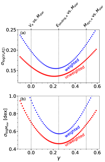
Figure 1: The dispersion of the best-fitted Equation 1 as a function of $\gamma$. (a) the dispersion in log($V_{\rm e}R_{\rm e}^{\gamma}$). (b) the dispersion in log($M_{\rm star}$). The unweighted dispersion is the standard deviation, while the weighted dispersion is the one weighted by the number of each galaxy type (see text). Three dotted lines mark $\gamma$ values at which $V_{\rm e}R_{\rm e}^{\gamma}$ represents the $V_{\rm e}$, the binding energy within $R_{\rm e}$ and the dynamical mass within $R_{\rm e}$, respectively, as illustrated in Equation 2.

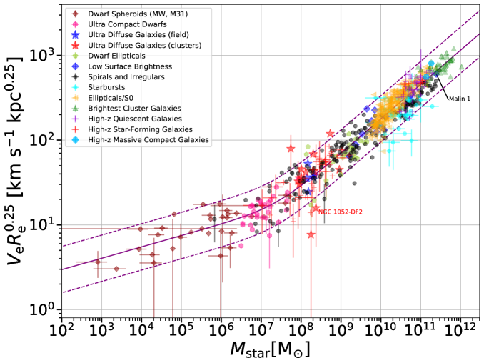
Figure 2: A relationship between stellar masses of galaxies ($M_{\rm star}$) and the product of the dynamical velocity and size to one fourth power both at the galaxy effective radius ($V_{\rm e}R_{\rm e}^{0.25}$). Types of galaxies are listed in Table 1. $V_{\rm e}R_{\rm e}^{0.25}$ represents the fourth root of the total binding energy within $R_{\rm e}$ of a galaxy (see text). The best-fit double power law is shown as a solid curve, while two dashed curves indicate $\pm$2$\sigma$. For clarity, error bars that are smaller than 0.15 dex are not plotted in the figure.

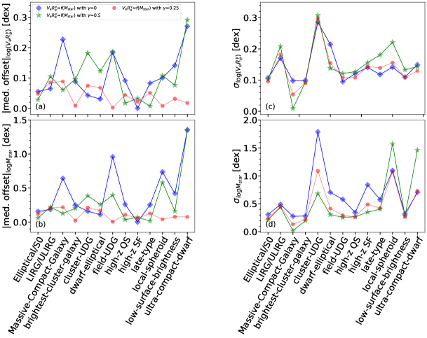
Figure 3: The median offsets and standard deviation of individual galaxy types. a, the median offset in log($V_{\rm e}R_{\rm e}^{\gamma}$). b, the standard deviation in log($V_{\rm e}R_{\rm e}^{\gamma}$). c, the median offset in log($M_{\rm star}$). d, the standard deviation of in log($M_{\rm star}$).

3 Results

3.1 Different combinations of $V_{\rm e}$ and $R_{\rm e}$ in correlations with $M_{\rm star}$

To find the best combination of $V_{\rm e}$ and $R_{\rm e}$ to correlate with $M_{\rm star}$, we employed the following double-power-law relationship between $V_{\rm e}R_{\rm e}^{\gamma}$ and $M_{\rm star}$:

$$V_{\rm e}R_{\rm e}^{\gamma}=A(M_{\rm star}/M_{0})^{\alpha}(1+M_{\rm star}/M_{0})^{\beta-\alpha}.$$ (1)

For each $\gamma$, we carried out the best fitting with the Python code scipy.optimize.curve_fit and estimated the dispersion of the derived correlation. Figure 1 shows the overall dispersion as a function of $\gamma$. Figure 2 gives an example of the above double-power-law relationship for $\gamma$=0.25.

At different ${\gamma}$, $V_{\rm e}R_{\rm e}^{\gamma}$ represents different physical properties of galaxies:

$$V_{\rm e}R_{\rm e}^{\gamma}=\begin{cases}V_{\rm e}&\gamma=0,\\ V_{\rm e}R_{\rm e}^{0.25}\propto(E_{\rm binding,e})^{0.25}&\gamma=0.25,\\ V_{\rm e}R_{\rm e}^{0.5}\propto(M_{\rm dyn,e})^{0.5}&\gamma=0.5,\\ \end{cases}$$ (2)

where $E_{\rm binding,e}$ is the binding energy within the effective radius and $M_{\rm dyn,e}$ is the dynamical mass within the effective radius. Here at $\gamma$=0.25 we show that

$$\begin{split}E_{\rm binding,e}&\approx\frac{GM_{\rm dyn,e}^{2}}{R_{\rm e}}\equiv\frac{R_{\rm e}V_{\rm e}^{4}}{G}\\ &=4.62\times 10^{48}\;{\rm erg}\left(\frac{V_{\rm e}R_{\rm e}^{0.25}}{\rm km\;s^{-1}\;kpc^{0.25}}\right)^{4}.\end{split}$$ (3)

Figure 1 (a) and (b) show the dispersion of log($V_{\rm e}R_{\rm e}^{\gamma}$) and the dispersion of log($M_{\rm star}$) as a function of $\gamma$, respectively. Two types of dispersions are measured: one is the standard deviation; another is weighted by the number of different galaxy types as $\sigma$ = (${\sum}\frac{({\rm obs}_{i}-{\rm pred}_{i})^{2}}{w_{i}}$/$\sum\frac{1}{w_{i}}$)^0.5, where $w_{i}$ is the total number of the galaxy type that a given galaxy belongs to. This latter dispersion is to balance the fact that different galaxy types have different number of objects in this study, so that the dispersion is not dominated by the galaxy type with a large number of objects. In Figure 1 (a), the minima of $\sigma_{{\rm log}(V_{\rm e}R_{\rm e}^{\gamma})}$ occur at $\gamma$=0.21 and 0.22  for unweighted and weighted cases, respectively. In Figure 1 (b), the minima of $\sigma_{{\rm log}(M_{\rm star})}$ are located at $\gamma$=0.25 for both weighted and unweighted cases.

3.2 A universal correlation between stellar masses and binding energies of galaxies

As shown in the above section, the stellar mass of a galaxy is best correlated with $V_{\rm e}R_{\rm e}^{\gamma}$ when $\gamma$ is around 0.25, i.e., the relationship has the minimum dispersion as compared to other combinations of $V_{\rm e}$ and $R_{\rm e}$. Since $V_{\rm e}R_{\rm e}^{0.25}$ represents the fourth root of the binding energy within the effective radius of a galaxy (Equation 2), we thus refer this correlation as the stellar mass-binding energy relationship. As shown in Figure 2, all galaxies together define a double power law function of

$$V_{\rm e}R_{\rm e}^{0.25}=A(M_{\rm star}/M_{0})^{\alpha}(1+M_{\rm star}/M_{0})^{\beta-\alpha},$$ (4)

with the best-fitted $A$=15.7$\pm$2.2 km s^-1 kpc^0.25, $M_{0}$=(2.5$\pm$1.0)$\times$10⁷ M_⊙, $\alpha$=0.134$\pm$0.020 and $\beta$=0.406$\pm$0.007. The whole relationship has standard deviation of 0.14 dex  in log($V_{\rm e}R_{\rm e}^{0.25}$) and 0.46 dex  in log($M_{\rm star}$). It covers a stellar mass range of nine orders of magnitude, from one-thousand-solar-mass dwarf spheroidal galaxies to the brightest galaxies in clusters with stellar masses of one-thousand-billion solar masses. As shown in Figure 3, the median offsets of individual galaxy types from the best fit are smaller than the standard deviation of the whole sample. Individual galaxy types have a small standard deviation too, except for ultra diffuse galaxies in clusters that have a standard deviation about two times that of the whole sample. Large observational errors account for at least a part of the large dispersion of these galaxies.

Figure 3 further compares the stellar mass-binding energy relationship (Equation 1 with $\gamma$=0.25) to the case with $\gamma$=0.5 that represents the relationship between the stellar mass and dynamical mass as shown in Figure 4. The latter relationship has an overall standard deviation of 0.18 dex  in log($V_{\rm e}R_{\rm e}^{\gamma}$) as shown in Figure 1, that is 30% larger than the stellar mass-binding energy relationship. A few types of galaxies show much larger systematic offsets: ultra compact dwarfs show a median offset in ${{\rm log}(V_{\rm e}R_{\rm e}^{\gamma})}$=0.27 dex  that is much larger than -0.018 dex  in the stellar mass-binding energy relationship; in addition, LIRGs/ULIRGs, ultra diffuse galaxies both in field and clusters, dwarf ellipticals, local spheroids all show median offsets in ${\rm log}(V_{\rm e}R_{\rm e}^{\gamma})$ larger than 0.1 dex, while none of a galaxy type shows such an offset in the stellar mass-binding energy relationship. As a result, the stellar mass-binding energy relationship should not be caused by the relationship between the stellar mass and dynamical mass.

Figure 3 also shows that in the case with $\gamma$=0 several galaxy types show median offsets in ${\rm log}(V_{\rm e}R_{\rm e}^{\gamma})$ larger than 0.1 dex, including massive compact galaxies, ultra diffuse galaxies in field, low surface brightness galaxies and ultra compact dwarfs. This suggests that the stellar mass-binding energy relationship is not caused by the relationship between the stellar mass and the dynamical velocity either.

The scatter of the stellar mass-binding energy relation shows no dependence on other galaxy properties. As shown in Figure 5 (a), the effective radii of the sample cover more than four orders of magnitude, ranging from about 5 pc seen in ultra compact dwarfs to about 70 kpc as seen in one of the largest galaxies – Malin 1. As shown in Figure 5 (b), the dynamical to stellar mass ratio within effective radii of the sample covers more than a factor of 10 if excluding local spheroidal galaxies that show much higher ratios. The environments of the sample range from the dense centers of galaxy clusters to isolated field, all of which show small offsets from the best fit. The star formation rate of our sample ranges from $<$ 0.01 solar mass per year to more than one hundred solar masses per year as seen in starburst galaxies (Bellocchi et al., 2013).

The redshift evolution of the stellar mass-binding energy correlation is negligible. High-redshift objects in our sample cover the redshift range from 0.17 to about 2.4. They are classified into three types including star-forming (Genzel et al., 2017; Miller et al., 2014), quiescent (Belli et al., 2014) and massive compact ones (van de Sande et al., 2011; van Dokkum et al., 2009). As shown in Figure 3 and listed in Table 1, the median offsets of all three types are smaller than the standard deviation of the whole sample.

Our sample contains individual objects that are outliers of other scaling laws of galaxies. Ultra diffuse galaxies in field are found to systematically deviate by about 0.35 dex in the velocity from the Tully-Fisher relationship (Mancera Piña et al., 2019; Shi et al., 2021), but they follow the stellar mass-binding energy relationship with a median offset of only $-0.002$ dex. NGC 1052-DF2, an ultra diffuse galaxy in cluster (van Dokkum et al., 2018), deviates from the stellar mass-total halo mass relationship by a factor of 400, while it deviates from the stellar mass-binding energy relationship by only a factor of 2.5. Star-forming galaxies at high redshift (Genzel et al., 2017) that lack dark matter also obey the relationship very well. Dwarf ellipticals define a different slope in the Faber-Jackson plane (Faber & Jackson, 1976) as compared to the one defined by ellipticals and ultra compact dwarfs (Drinkwater et al., 2003; de Rijcke et al., 2005; Chilingarian et al., 2008), or equivalently showing on average about 0.4 dex offset in the velocity dispersion. But they do follow the stellar mass-binding energy relationship with a median offset of $-0.068$ dex.

3.3 A comparison to the fundamental plane of elliptical galaxies

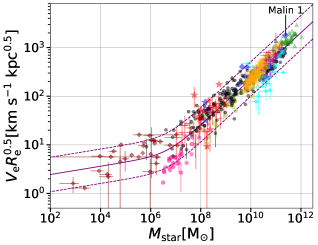
Figure 4: $V_{\rm e}R_{\rm e}^{0.5}$ that represents the square root of the dynamical mass within $R_{\rm e}$, as a function of the galaxy stellar mass. For clarity, error bars that are smaller than 0.15 dex are not plotted in all panels. Symbols represent different galaxy types as shown in Figure 2. The best-fit double power law is shown as a solid curve, while two dashed curves indicate $\pm$2$\sigma$.

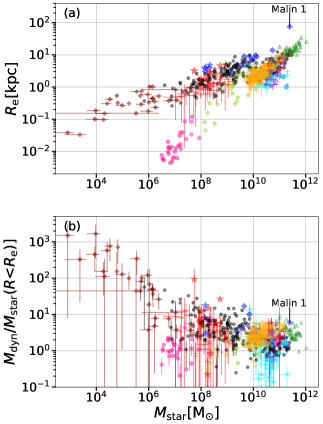
Figure 5: (a) The galaxy effective radius as a function of the galaxy stellar mass. (b) The dynamical to stellar mass ratio within effective radii as a function of the galaxy stellar mass. For clarity, error bars that are smaller than 0.15 dex are not plotted in all panels. Symbols represent different galaxy types as shown in Figure 2.

Figure 6: a, The distribution of all galaxies of this study in the fundamental plane of ellipticals. b, The distribution of $-(1+2c)/b$ in Equation 6 that represents $\gamma$ in Equation 1 by different studies of ellipticals.

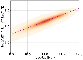
Figure 7: The distribution of $\sim$ 370,000 SDSS early-type galaxies in the stellar mass-binding energy relationship. The standard deviation in log($V_{\rm e}R_{\rm e}^{0.25}$) is 0.09 dex. The solid line is not the fitting to the SDSS data but the best fit from Figure 2.

The fundamental plane of elliptical galaxies invokes the same three physical parameters as the stellar mass-binding energy relation does in this study. The fundamental plane is generally written as

$${\rm log}R_{\rm 2D,e}=a+b\,{\rm log}\sigma_{0}+c\,{\rm log}\Sigma_{\rm e},$$ (5)

where $R_{\rm 2D,e}$ is the 2-D effective radius, $\sigma_{0}$ is the central velocity dispersion and $\Sigma_{\rm e}$ is the effective surface brightness in optical or near-IR. The equation can be transformed into

$${M_{\rm star}}\propto V_{\rm e}^{(-b/c)}R_{\rm e}^{(1+2c)/c}=(V_{\rm e}R_{\rm e}^{-(1+2c)/b})^{(-b/c)}.$$ (6)

Here $M_{\rm star}$ represents the stellar light, $V_{\rm e}$ represents the $\sigma_{0}$ and 3-D $R_{\rm e}$ represents the $R_{\rm 2D,e}$, all of which has a small dispersion that should not affect the derived power indices (see § 2.1). By adopting $b$=1.063$\pm$0.041 and $c$=$-$0.765$\pm$0.023 as derived by Cappellari et al. (2013) for ellipticals used in this study, Figure 6 (a) shows the distribution of all our galaxies in the fundamental plane. As expected, it clearly shows that the fundamental plane only holds for ellipticals but not other types of galaxies.

It has been known that the fundamental plane of ellipticals can be inferred through virial equilibrium, or it is essentially a relationship between the stellar mass and dynamical mass. To confirm this, Figure 6 (b) plots the distribution of $-(1+2c)/b$ that represents $\gamma$ in Equation 1 from different studies of the fundamental plane (Dressler et al., 1987; Djorgovski & Davis, 1987; Lucey et al., 1991; Guzman et al., 1993; Jorgensen et al., 1996; Hudson et al., 1997; Scodeggio, 1997; Pahre et al., 1998; Mobasher et al., 1999; Kelson et al., 2000; Gibbons et al., 2001; Colless et al., 2001; Bernardi et al., 2003; Cappellari et al., 2013). As shown in the figure, the $-(1+2c)/b$ is between 0.35 and 0.6, with a median and standard deviation of 0.48$\pm$0.07. That is close to $\gamma{\equiv}$0.5 when Equation 1 represents a relationship between the stellar mass and dynamical mass, while significantly different from $\gamma{\equiv}$0.25 when Equation 1 represents a relationship between the stellar mass and binding energy. We further fitted our galaxies by excluding local spheroidal galaxies with Equation 5 to avoid the bending at the low mass end through the Python code statsmodels.api.OLS. It is found that $a$=2.416$\pm$0.088, $b$=1.569$\pm$0.028, $c$=-0.645$\pm$0.013 for the case that $M_{\rm star}$ represents the stellar light, $V_{\rm e}$ represents the $\sigma_{0}$ and 3-D $R_{\rm e}$ represents the $R_{\rm 2D,e}$. This gives $-(1+2c)/b$ of about 0.2, supporting a physical link between stellar masses and binding energies if including galaxy types in addition to ellipticals.

It is thus clear that elliptical galaxies show the smallest dispersion around $\gamma=0.5$, while all galaxy types together define a tight sequence around $\gamma=0.25$. We further made a comparison in the dispersion of log$R_{\rm e}$ for ellipticals when forcing $-(1+2c)/b$=0.5 and $-(1+2c)/b$=0.25 in Equation 5. By varying $c$ over a large range of -2 to 1, it is found that the smallest dispersion in log$R_{\rm e}$ of the former, that is 0.10 dex, is smaller than the latter by only 3%. We also confirmed a similar difference with a large sample of $\sim$ 370,000 elliptical galaxies. These objects were selected from SDSS value-added catalog with FRACDEV_R $>$ 0.8 and MSTAR_TOT $>$ 10 (Kauffmann et al., 2003; Brinchmann et al., 2004). We used the total stellar mass MSTAR_TOT, V_DISP multiplied with $\sqrt{5/2}$ as $V_{\rm e}$ and PETROR50_R multiplied with 4/3 as $R_{\rm e}$.

As a summary, the fundamental plane of ellipticals represents the relationship between the stellar mass and dynamical mass, which is physically different from the stellar mass-binding energy relationship in this study. The former is only valid for ellipticals, and its dispersion in log$R_{\rm e}$ is only slightly smaller than the dispersion of ellipticals in the stellar mass-binding energy relationship. Figure 7 further shows the distribution of SDSS early type galaxies in the plane of the stellar mass vs. the binding energy. As shown in the figure, they lie well on the best fit to galaxies in Figure 2. The standard deviation in log($V_{\rm e}R_{\rm e}^{0.25}$) of Figure 7 is found to be 0.09 dex.

4 Discussions

4.1 Comparisons with other relationships

Under some circumstances, the stellar mass-binding energy relationship can be transformed to a linear relationship between the galaxy size and halo size, a result expected in a scenario that the specific angular momenta of haloes are the same as those of galaxies (Fall & Efstathiou, 1980; Mo et al., 1998). In the case where the dynamical velocity is dominated by the gravity of dark matter at the effective radius, $V_{\rm e}$=$V_{200}g(c,x)$=$R_{200}hg(c,x)$, where $h$ is Hubble constant of 100 km s^-1 Mpc^-1, $R_{200}$ is the halo radius in kpc and $g(c,x)$=$\sqrt{\frac{{\rm ln}(1+cx)-cx/(1+cx)}{x[{\rm ln}(1+c)-c/(1+c)]}}$. For $c$ in the range of [3, 30] (Macciò et al., 2007) and $x$ in the range of [0.001, 0.1] (Kravtsov, 2013), it can be shown that $g(c,x)$$\approx$1.74$x^{0.42}c^{0.3}$ with standard deviation of 0.1 dex. From Equation 4 when $M_{\rm star}$ is much larger than $M_{0}$, we got

$$\begin{split}R_{\rm e}\;&\approx\;0.014R_{200}[\frac{7.24(M_{\rm star}/5{\times}10^{10}M_{\odot})^{0.32}}{R_{\rm e}}]^{-2.31}(c/6)^{0.53}\\ &\approx\;0.014R_{200}(c/6)^{0.53},\end{split}$$ (7)

if assuming $R_{\rm e}$ = 7.24 kpc $(M_{\rm star}/5{\times}10^{10}M_{\odot})^{0.31}$ whose power index is 20% steeper than the observation (van der Wel et al., 2014). The derived galaxy size-halo size linear relationship is then quite close to the one that is obtained from the abundance matching (Kravtsov, 2013). A key difference is that our estimate shows a dependence on the concentration of the halo.

The Tully-Fisher relationship (Tully & Fisher, 1977) of late-type galaxies and Faber-Jackson relationship (Faber & Jackson, 1976) of early-type galaxies are independent of our stellar mass-binding energy correlation as the former two are essentially the relationship between the halo mass and stellar mass. But the latter can be transformed to the former two by assuming certain functions of galaxy sizes with their stellar masses. For the Tully-Fisher relationship, we used the above conversion from $V_{\rm e}$ to $V_{200}$ and found $M_{\rm star}$ $\propto$ $V_{200}^{3.7}$ (Lelli et al., 2016), if adopting $R_{\rm e}$ $\propto$ $M_{\rm star}^{0.35}$ whose power index is 40% steeper than the observation (van der Wel et al., 2014). For the Faber-Jackson law, the stellar mass is found to be proportional to the velocity dispersion at the effective radius to the power index of 4.0 (Drinkwater et al., 2003), if adopting $R_{\rm e}$ $\propto$ $M_{\rm star}^{0.58}$ whose power index is 20% smaller than the observation (van der Wel et al., 2014).

4.2 A toy model of self regulation

The tight correlation in Figure 2 points to the universal role of the binding energies of galaxies in the evolution of stellar masses. The binding energy within the effective radius may set a threshold above which stars/gas cannot survive by being expelled out of galaxies. Studies of galaxy formation and evolution have recognized many mechanisms that affect energies of gas and stars. Some are negative by increasing the energies such as ram pressuring, tidal stripping, supernova feedback etc. Some are positive by removing the energies such as cooling, turbulence etc. In a galaxy with a higher threshold, positive mechanisms work efficiently to accumulate more gas and stars while the effects of negative mechanisms are minimized, so that a more massive galaxy forms or survives, and vice versa for a halo with a lower threshold.

To reproduce the observed slopes of the stellar mass-binding energy relationship, we present a toy model of self-regulation feedback where binding energies of galaxies self-balance the energies of stellar systems that have been injected by supernovae feedback over the galaxy history. We have

$$E_{\rm binding,e}\approx E_{\rm tot{-}SN}.$$ (8)

The supernovae event per time can be written as a function of the galaxy stellar mass (Graur et al., 2015):

$$R_{\rm SN}=\frac{dN_{\rm SN}}{dt}\;{\propto}\;M_{\rm star}^{1+B}.$$ (9)

Supernovae continuously inject energies into the interstellar media that form stars over the galaxy history. The deposited energy is proportional to the number of gas particles that is the gas mass, so that the final energies of stellar systems injected by supernova are

$$E_{\rm tot{-}SN}\;{\propto}\int R_{\rm SN}\,dM_{\rm gas}\;{\propto}\int R_{\rm SN}\,({\rm SFR})\,dt=\int R_{\rm SN}\,dM_{\rm star}$$ (10)

Here we assume a linear relationship between the star formation rate (SFR) and gas mass (Gao & Solomon, 2004) instead of other relationships (Kennicutt, 1998; Shi et al., 2014, 2018), since only energies that inject into star-forming gas contribute to the final energies of stellar systems. The combination of the above two equations gives

$$E_{\rm tot{-}SN}\;{\propto}M_{\rm star}^{B+2}$$ (11)

The observations give $B$ around $-0.5$ for both type I and type II supernova (Graur et al., 2015), so that we have $E_{\rm binding,e}$ ${\propto}$ $M_{\rm star}^{1.5}$, which is close to the slope (4$\beta$ $\sim$ 1.62) we observe above $M_{0}$ as seen in Equation 4.

As shown in Figure 2, extremely low mass galaxies show a different slope as compared to those above the $M_{0}$. This may be because in these tiny galaxies the feedback is so efficient so that only a small amount of gas and stars can sustain (Wetzel et al., 2016). A typical $V_{\rm e}R_{\rm e}^{0.25}$ of these low mass galaxies is about 5 km s^-1 kpc^0.25, giving the galaxy binding energy $E_{\rm binding,e}$ of 2.9$\times$10⁵¹ erg. This is a typical energy of a single supernova event, meaning that a single supernova explosion may be powerful enough to disrupt the galaxy. In this case, no integration in Equation 10 gives $E_{\rm tot{-}SN}$ $\propto$ $R_{\rm SN}$, and so that $E_{\rm binding,e}$ $\propto$ $M_{\rm star}^{0.5}$ whose power index on $M_{\rm star}$ is also close to the slope (4$\alpha$ $\sim$ 0.54) that we observe below $M_{0}$ in Equation 4.

The above self-regulation scenario requires a thorough mixing in kinematics among stars, gas and dark matters so that the initially released energy into the stellar system is equal to the final binding energy of all particles within the effective radius, instead of only the part of stars.

This toy model emphasizes the history of the stellar growth through which star-forming gas continuously receives feedback from supernovae, while the feedback from active galactic nuclei most likely plays its major role in terminating star formation at the final stage of the stellar growth. This may explain why the slope of the relationship can be produced without invoking feedback from active galactic nuclei.

It should be pointed out that this toy model illustrates one example about the interplay between galaxy binding energies and their stellar masses. The underlying physical mechanisms may be much more complicated. An in-depth comparison with simulations may give some key insights.

4.3 Some potential applications

The universality of the stellar mass-binding energy relationship makes it potential a distance estimator, especially that it is independent of galaxy types and shows little redshift evolution. For stellar masses above $M_{0}$, the luminosity distance is given by $D_{\rm L}$ = 155 Mpc $(\frac{V_{\rm e}}{\rm km/s})^{1.78}(1+z)^{-0.89}M_{\rm star,Mpc}^{-0.72}(\frac{R_{\rm e}}{\rm arcsec})^{0.44}$, where $M_{\rm star,Mpc}$ is the stellar mass at a luminosity distance of 1 Mpc. The 1-$\sigma$ uncertainty is 0.2 dex for individual distance estimates. As compared to the Tully-Fisher relationship, it has an advantage by measuring the velocity at the effective radius instead of that at the outer flat part of the rotation curve.

The universality of the relationship also challenges the modified Newtonian dynamics (Milgrom, 1983), which has a form of $VR^{0.5}$ $\propto$ $M_{\rm star}^{0.5}$ at the high acceleration regime and $V$ $\propto$ $M_{\rm star}^{0.25}$ at the low acceleration regime, none of which fits Equation 4.

5 Conclusions

In this study, it is found that the galaxy stellar mass is universally correlated with $V_{\rm e}R_{\rm e}^{\gamma}$ when $\gamma$=0.25. The $V_{\rm e}R_{\rm e}^{0.25}$ represents the fourth root of the total binding energies of galaxies including dark matter and baryons within the galaxy effective radii. The stellar mass-binding energy correlation holds for a variety of galaxy types and shows a standard deviation of 0.14 dex  in log($V_{\rm e}R_{\rm e}^{0.25}$) and 0.46 dex  in log($M_{\rm star}$), with little redshift evolution. It is physically different from the fundamental plane of ellipticals that represents the relation between the stellar mass and dynamical mass. A toy model of self-regulation between binding energies and supernovae feedback is proposed to reproduce the observed slopes of the correlation. The relationship can also be used to estimate the distance of a galaxy with an uncertainty of 0.2 dex, independent of the galaxy type.

Data Availability

All the data used here are available upon reasonable request.

References

- Beasley et al. (2016) Beasley M. A., Romanowsky A. J., Pota V., Navarro I. M., Martinez Delgado D., Neyer F., Deich A. L., 2016, ApJ, 819, L20
- Belli et al. (2014) Belli S., Newman A. B., Ellis R. S., 2014, ApJ, 783, 117
- Bellocchi et al. (2013) Bellocchi E., Arribas S., Colina L., Miralles-Caballero D., 2013, A&A, 557, A59
- Bernardi et al. (2003) Bernardi M., et al., 2003, AJ, 125, 1866
- Bothun et al. (1987) Bothun G. D., Impey C. D., Malin D. F., Mould J. R., 1987, AJ, 94, 23
- Brinchmann et al. (2004) Brinchmann J., Charlot S., White S. D. M., Tremonti C., Kauffmann G., Heckman T., Brinkmann J., 2004, MNRAS, 351, 1151
- Cappellari et al. (2006) Cappellari M., et al., 2006, MNRAS, 366, 1126
- Cappellari et al. (2011) Cappellari M., et al., 2011, MNRAS, 413, 813
- Cappellari et al. (2013) Cappellari M., et al., 2013, MNRAS, 432, 1709
- Chilingarian et al. (2008) Chilingarian I. V., Cayatte V., Durret F., Adami C., Balkowski C., Chemin L., Laganá T. F., Prugniel P., 2008, A&A, 486, 85
- Chilingarian et al. (2019) Chilingarian I. V., Afanasiev A. V., Grishin K. A., Fabricant D., Moran S., 2019, ApJ, 884, 79
- Colless et al. (2001) Colless M., Saglia R. P., Burstein D., Davies R. L., McMahan R. K., Wegner G., 2001, MNRAS, 321, 277
- Dey et al. (2019) Dey A., et al., 2019, AJ, 157, 168
- Djorgovski & Davis (1987) Djorgovski S., Davis M., 1987, ApJ, 313, 59
- Dressler et al. (1987) Dressler A., Lynden-Bell D., Burstein D., Davies R. L., Faber S. M., Terlevich R., Wegner G., 1987, ApJ, 313, 42
- Drinkwater et al. (2003) Drinkwater M. J., Gregg M. D., Hilker M., Bekki K., Couch W. J., Ferguson H. C., Jones J. B., Phillipps S., 2003, Nature, 423, 519
- Faber & Jackson (1976) Faber S. M., Jackson R. E., 1976, ApJ, 204, 668
- Fall & Efstathiou (1980) Fall S. M., Efstathiou G., 1980, MNRAS, 193, 189
- Forbes et al. (2014) Forbes D. A., Norris M. A., Strader J., Romanowsky A. J., Pota V., Kannappan S. J., Brodie J. P., Huxor A., 2014, MNRAS, 444, 2993
- Gao & Solomon (2004) Gao Y., Solomon P. M., 2004, ApJS, 152, 63
- Genzel et al. (2017) Genzel R., et al., 2017, Nature, 543, 397
- Gibbons et al. (2001) Gibbons R. A., Fruchter A. S., Bothun G. D., 2001, AJ, 121, 649
- Graur et al. (2015) Graur O., Bianco F. B., Modjaz M., 2015, MNRAS, 450, 905
- Guzman et al. (1993) Guzman R., Lucey J. R., Bower R. G., 1993, MNRAS, 265, 731
- Hudson et al. (1997) Hudson M. J., Lucey J. R., Smith R. J., Steel J., 1997, MNRAS, 291, 488
- Impey et al. (1996) Impey C. D., Sprayberry D., Irwin M. J., Bothun G. D., 1996, ApJS, 105, 209
- Jorgensen et al. (1996) Jorgensen I., Franx M., Kjaergaard P., 1996, MNRAS, 280, 167
- Kauffmann et al. (2003) Kauffmann G., et al., 2003, MNRAS, 341, 33
- Kelson et al. (2000) Kelson D. D., Illingworth G. D., van Dokkum P. G., Franx M., 2000, ApJ, 531, 184
- Kennicutt (1998) Kennicutt Robert C. J., 1998, ApJ, 498, 541
- Kravtsov (2013) Kravtsov A. V., 2013, ApJ, 764, L31
- Lelli et al. (2010) Lelli F., Fraternali F., Sancisi R., 2010, A&A, 516, A11
- Lelli et al. (2016) Lelli F., McGaugh S. S., Schombert J. M., 2016, AJ, 152, 157
- Loubser et al. (2008) Loubser S. I., Sansom A. E., Sánchez-Blázquez P., Soechting I. K., Bromage G. E., 2008, MNRAS, 391, 1009
- Lucey et al. (1991) Lucey J. R., Bower R. G., Ellis R. S., 1991, MNRAS, 249, 755
- Macciò et al. (2007) Macciò A. V., Dutton A. A., van den Bosch F. C., Moore B., Potter D., Stadel J., 2007, MNRAS, 378, 55
- Mancera Piña et al. (2019) Mancera Piña P. E., et al., 2019, ApJ, 883, L33
- Mieske et al. (2008) Mieske S., et al., 2008, A&A, 487, 921
- Milgrom (1983) Milgrom M., 1983, ApJ, 270, 365
- Miller et al. (2014) Miller S. H., Ellis R. S., Newman A. B., Benson A., 2014, ApJ, 782, 115
- Mo et al. (1998) Mo H. J., Mao S., White S. D. M., 1998, MNRAS, 295, 319
- Mobasher et al. (1999) Mobasher B., Guzman R., Aragon-Salamanca A., Zepf S., 1999, MNRAS, 304, 225
- Oman et al. (2016) Oman K. A., Navarro J. F., Sales L. V., Fattahi A., Frenk C. S., Sawala T., Schaller M., White S. D. M., 2016, MNRAS, 460, 3610
- Pahre et al. (1998) Pahre M. A., de Carvalho R. R., Djorgovski S. G., 1998, AJ, 116, 1606
- Peebles (1969) Peebles P. J. E., 1969, ApJ, 155, 393
- Persic et al. (1996) Persic M., Salucci P., Stel F., 1996, MNRAS, 281, 27
- Posti et al. (2018) Posti L., Fraternali F., Di Teodoro E. M., Pezzulli G., 2018, A&A, 612, L6
- Read et al. (2017) Read J. I., Iorio G., Agertz O., Fraternali F., 2017, MNRAS, 467, 2019
- Schombert et al. (2019) Schombert J., McGaugh S., Lelli F., 2019, MNRAS, 483, 1496
- Scodeggio (1997) Scodeggio M., 1997, PhD thesis, CORNELL UNIVERSITY
- Shi et al. (2014) Shi Y., Armus L., Helou G., Stierwalt S., Gao Y., Wang J., Zhang Z.-Y., Gu Q., 2014, Nature, 514, 335
- Shi et al. (2018) Shi Y., et al., 2018, ApJ, 853, 149
- Shi et al. (2021) Shi Y., Zhang Z.-Y., Wang J., Chen J., Gu Q., Yu X., Li S., 2021, ApJ, 909, 20
- Tollerud et al. (2012) Tollerud E. J., et al., 2012, ApJ, 752, 45
- Toloba et al. (2012) Toloba E., Boselli A., Peletier R. F., Falcón-Barroso J., van de Ven G., Gorgas J., 2012, A&A, 548, A78
- Tully & Fisher (1977) Tully R. B., Fisher J. R., 1977, A&A, 500, 105
- U et al. (2012) U V., et al., 2012, ApJS, 203, 9
- Wetzel et al. (2016) Wetzel A. R., Hopkins P. F., Kim J.-h., Faucher-Giguère C.-A., Kereš D., Quataert E., 2016, ApJ, 827, L23
- Wolf et al. (2010) Wolf J., Martinez G. D., Bullock J. S., Kaplinghat M., Geha M., Muñoz R. R., Simon J. D., Avedo F. F., 2010, MNRAS, 406, 1220
- Zhang et al. (2012) Zhang H.-X., Hunter D. A., Elmegreen B. G., Gao Y., Schruba A., 2012, AJ, 143, 47
- de Blok et al. (2001) de Blok W. J. G., McGaugh S. S., Rubin V. C., 2001, AJ, 122, 2396
- de Rijcke et al. (2005) de Rijcke S., Michielsen D., Dejonghe H., Zeilinger W. W., Hau G. K. T., 2005, A&A, 438, 491
- van Dokkum et al. (2009) van Dokkum P. G., Kriek M., Franx M., 2009, Nature, 460, 717
- van Dokkum et al. (2016) van Dokkum P., et al., 2016, ApJ, 828, L6
- van Dokkum et al. (2018) van Dokkum P., et al., 2018, Nature, 555, 629
- van Dokkum et al. (2019) van Dokkum P., et al., 2019, ApJ, 880, 91
- van de Sande et al. (2011) van de Sande J., et al., 2011, ApJ, 736, L9
- van der Wel et al. (2014) van der Wel A., et al., 2014, ApJ, 788, 28