Sensitivity Approximation by the Peano-Baker Series

Abstract

In this paper we develop a new method for numerically approximating sensitivities in parameter-dependent ordinary differential equations (ODEs). Our approach, intended for situations where the standard forward and adjoint sensitivity analysis become too computationally costly for practical purposes, is based on the Peano-Baker series from control theory. We give a representation, using this series, for the sensitivity matrix $\mathbf{S}$ of an ODE system and use the representation to construct a numerical method for approximating $\mathbf{S}$. We prove that, under standard regularity assumptions, the error of our method scales as $O(\Delta t^{2}_{max})$, where $\Delta t_{max}$ is the largest time step used when numerically solving the ODE. We illustrate the performance of the method in several numerical experiments, taken from both the systems biology setting and more classical dynamical systems. The experiments show the sought-after improvement in running time of our method compared to the forward sensitivity approach. For example, in experiments involving a random linear system, the forward approach requires roughly $\sqrt{n}$ longer computational time, where $n$ is the dimension of the parameter space, than our proposed method.

Key words and phrases: Sensitivity analysis; Peano-Baker series; ordinary differential equations; error analysis.

MSC 2010 subject classifications: 65L05; 65L20.

1 Introduction

Mathematical models are used in all areas of science and engineering to model more and more complex real-world phenomena. An important aspect of such modeling is to understand how changes and uncertainty in model parameters translate to the output of a model. The first question is the topic of sensitivity analysis, an active research area at the intersection of several branches of mathematics and its applications; see e.g. [11, 8, 4, 21, 5] and references therein. Motivated by problems arising in systems biology, specifically concerning statistical inference and uncertainty quantification for models based on non-linear dynamical systems, in this paper we consider the rather classical question of local sensitivity analysis in ODE models. More precisely, we are interested in the design of efficient numerical methods for approximating the sensitivity matrix for such models.

The general starting point is a system of ordinary differential equations (ODEs), which we take to be of the form

$$\begin{cases}\dot{\mathbf{x}}(t)=f(\mathbf{x}(t),\mathbf{u}(t),\mathbf{p}),\\ \mathbf{x}(t_{0})=\mathbf{x}_{0},\end{cases}$$

where $\mathbf{x}(t)$ represents the state of the system at time $t$, $\mathbf{u}$ corresponds to external inputs into the system and $\mathbf{p}$ denotes a set of model parameters; a more precise definition, including the state spaces of the different quantities involved, is given in Section 2. For such a model, it is important to understand how changes in the parameter-vector $\mathbf{p}$ affect the output $\mathbf{x}$. We are interested in computing the derivatives $\partial x_{i}(t)/\partial p_{j}$, the sensitivities of the model, for all component-combinations $x_{i},p_{j}$. The sensitivities provide local information about the parameter space important for a variety of tasks within modeling where this space is explored, e.g., quantifying uncertainty, finding optimal parameters and experimental design [8, 4, 5, 6].

For all but very simple systems the sensitivities are not available in an (explicit) analytical form. Instead we have to turn to different types of approximations [4, 5]. The two standard approaches for obtaining numerical approximations to the sensitivities of an ODE or PDE model are (i) the forward, or variational approach [8, 4], and (ii) the adjoint approach [17, 18, 7]. There is a vast literature on both methods and here we only give a brief review; for a comparison of the two approaches, see [6].

Forward sensitivity analysis is the more straightforward method of the two. It is based on finding an ODE system satisfied by the sensitivities $\partial x_{i}(t)/\partial p_{j}$, along with appropriate initial values. The solution to this system can then be approximated together with that of the original ODE for $\mathbf{x}$ [4, 6]. It is well-known that for high-dimensional problems — $n_{x}\times n_{p}\gg 1$, where $n_{x}$ and $n_{p}$ are the dimension of the state space and parameter space, respectively — computation of the sensitivities with the forward sensitivity analysis becomes slow. As a consequence, this method can be too computationally costly for certain applications, and more efficient methods are needed.

Adjoint sensitivity analysis is designed to ease the computation of sensitivities with respect to $\mathbf{p}$ of an objective function

$$G(\mathbf{x},\mathbf{p})=\int_{0}^{T}g(\mathbf{x},t,\mathbf{p})dt,$$

for some function $g$ (certain smoothness assumptions are necessary for $g$). Alternatively, the method can be used to compute sensitivities of $g(\mathbf{x}(T),T,\mathbf{p})$, that is a function only defined at the final time $T$. The method amounts to introducing an augmented objective function from $G$ by introducing Lagrange multipliers associated with the underlying ODE, and computing the derivatives $dG/dp_{j}$ of this objective function; see e.g. [7, 17, 18] for the details.

In contrast to the forward sensitivity analysis, the adjoint method does not rely on the actual state sensitivities, $\partial x_{i}/\partial p_{j}$, but rather on the adjoint state process. It is possible, albeit impractical, to formulate the problem so that the adjoint sensitivity analysis computes $\partial x_{i}/\partial p_{j}$, the quantities of interest in this paper: define $g(\mathbf{x},t,\mathbf{p})=x_{i}(t)$ and use the adjoint sensitivity method to compute the sensitivities of $g$ at the specific times $T=t_{k}$. However, this must be repeated for each component $x_{i}$ of the state $\mathbf{x}$ and for each time $t_{k}$ at which an approximation of the sensitivity of the ODE model is sought. As a result, the use of adjoint sensitivity is not recommended for this purpose, especially when (i) the dimension of the state space is large, and (ii) there are many time points $t_{k}$ at which the sensitivities are to be computed.

Before moving to the general setting and problem formulation, we expand briefly on our particular motivation for looking at this problem; note that although our original motivation comes from systems biology, the problem of computing sensitivities in an ODE model is of great interest in a number of fields.

Our motivation comes from uncertainty quantification for models of intracellular pathways, such as those studied in [10]. In this setting, the state process $\mathbf{x}(t)$ corresponds to the concentration of different compounds internal to the cell (e.g.  proteins or protein complexes like CaMKII or PP2B, or calcium ions), and the parameters $\mathbf{p}=(p_{1},\dots,p_{n_{p}})$ encode e.g. rate constants of the chemical reactions involved in the system. We are interested in uncertainty quantification for the unknown parameters in a Bayesian setting. This requires computing posterior distributions, which in turn requires Markov chain Monte Carlo (MCMC) methods. Recent developments in the MCMC community propose to take a (differential-) geometric perspective on sampling, exploiting potential underlying geometrical concepts related to statistical inference [13, 12, 2]. This relies on an appropriate choice of the metric tensor on the parameter space and a particular choice of interest is the expected Fisher information [13]: for a generic random variable $Y$ and associated parameter $\theta$, with conditional density $p_{Y|\theta}$, the expected Fisher information is defined as

$$F(\theta)=-E_{Y|\theta}\left[\frac{\partial^{2}}{\partial\theta^{2}}\log\left(p_{Y|\theta}(Y|\theta)\right)\right].$$

When combined with an ODE model, the entries of $F$ contain the sensitivities of the model and to efficiently implement corresponding MCMC methods, we first need an efficient method for repeatedly computing the corresponding sensitivities. Forward sensitivity analysis is too slow and because the full sensitivity matrix (see Section 2 for the definition) is required, the adjoint sensitivity analysis is not appropriate for this type of problem. We therefore propose a new method, based on the Peano-Baker series, that can resolve the issue of computational burden; using the method in the context of MCMC sampling is ongoing work and in this paper we consider the method solely from a numerical analysis perspective.

The method is based on the representations of the sensitivity matrix given in Theorem 2 and Corollary 1, and is outlined in Algorithms 1, 2 and 3. The main theoretical result of the paper is Theorem 3, which gives the error rate of the proposed method in terms of the time discretisation used for solving the underlying ODE. The theoretical results are complemented by numerical experiments and comparison to the forward sensitivity analysis shows significant improvement.

The remainder of the paper is organised as follows. In Section 2 we give a precise formulation of the ODE model and the associated sensitivities of interest. Next, in Section 3 we derive analytical representations of the sensitivities in two different cases: when the solution is at equilibrium, and in the general case. In Section 4 the analytical representations are used to propose a new method for approximating sensitivities in the ODE setting considered here. An error analysis of the proposed method is given in Section 5 and in Section 6 we present some numerical experiments that showcase the performance of the method. In particular we compare our method with the forward sensitivity approach and show superior performance. We end the paper with a brief discussion in Section 7.

1.1 Notation

The following notation is used. Elements in $\mathbb{R}^{n}$ are denoted by bold font, e.g. $\mathbf{x},\mathbf{y},\mathbf{z}$, whereas $x,y,z$ denote elements of $\mathbb{R}$; note that the relevant dimension $n$ will change between different vectors. With some abuse of notation, $0$ denotes the zero element in $\mathbb{R}^{n}$ for any $n\geq 1$. The identity matrix is denoted by $\mathbf{I}$, or $I_{n}$ whenever we want to emphasise the size $n\times n$. For a matrix $\mathbf{A}$, the matrix exponential $e^{\mathbf{A}}$ is defined in the usual way:

$$e^{\mathbf{A}}=\sum_{h\geq 0}\frac{1}{h!}\mathbf{A}^{h}.$$

Objects with a hat, such as $\hat{f}$ or $\hat{\mathbf{x}}$, refer to approximations.

For $k\in\mathbb{N}$ and an open set $A$ in $\mathbb{R}^{n}$, $C^{k}(A;\mathbb{R}^{m})$ is the space of continuous functions on $A$, taking values in $\mathbb{R}^{m}$, with continuous partial derivatives up to the $k$th order; for $m\geq 2$, the latter is defined in the usual way through natural projections. For a compact set $K$, $C^{k}(K;\mathbb{R}^{m})$ refers to functions that are $C^{k}(A;\mathbb{R}^{m})$ on some open neighbourhood $A$ of $K$. For a function $f:\mathbb{R}^{n}\to\mathbb{R}^{m}$, $\nabla f$ denotes the Jacobian matrix of $f$. For a normed space $(\mathcal{X},||\cdot||)$, $C^{0}([0,T];\mathcal{X})$ denotes the space of continuous functions from $[0,T]$ to $\mathcal{X}$ and $||\cdot||_{[0,T]}$ denotes the supremum norm over this space: for $g\in C^{0}([0,T];\mathcal{X})$,

$$||g||_{[0,T]}=\sup_{t\in[0,T]}||g(t)||.$$

Unless otherwise stated, we will let $||\cdot||$ denote an arbitrary matrix norm; because we are working on a finite-dimensional space, the specific choice of matrix norm is not important for the results of this paper (discussed more in Section 5). Additional notation that is particular to this work is defined as needed, particularly in the error analysis in Section 5.

2 Problem formulation

The general problem of interest is to compute sensitivities for the solution of the parametrised initial value problem (IVP)

$$\begin{cases}\dot{\mathbf{x}}(t)=f(\mathbf{x}(t),\mathbf{u}(t),\mathbf{p}).\\ \mathbf{x}(t_{0})=\mathbf{x}_{0}.\end{cases}$$ (1)

Here, for each $t\geq t_{0}$, the solution $\mathbf{x}(t)$ and control $\mathbf{u}(t)$ are in $\mathbb{R}^{n_{x}}$ and $\mathbb{R}^{n_{u}}$, respectively, and the parameter vector $\mathbf{p}$ is in $\mathbb{R}^{n_{p}}$. As noted in Section 1, although our interest in this problem comes from a desire to conduct uncertainty quantification for models in systems biology, the problem is much more general and arises in a wide variety of areas within applied mathematics. We therefore work in a general framework for the remainder of this paper.

To avoid issues with the existence or uniqueness of solutions, we make the following assumption; we have not aimed for generality and the assumptions put forth in the paper can most likely be weakened considerably in specific settings.

Assumption.

The function $f:\mathbb{R}^{n_{x}}\times\mathbb{R}^{n_{u}}\times\mathbb{R}^{n_{p}}\to\mathbb{R}^{n_{x}}$ is uniformly globally Lipschitz in the first coordinate given any choices of $\mathbf{u}$ and $\mathbf{p}$.

This assumption is made throughout the paper, without being referred to explicitly in the upcoming sections.

Definition 1.

Given a solution $\mathbf{x}$ of the ODE system (1), the sensitivity at time $t$ of the $l$-th component of $\mathbf{x}$ with respect to parameter $p_{i}$ is defined as

$$S_{l}^{~{}i}(t)=\frac{\partial x_{l}(t)}{\partial p_{i}},\quad l=1,\dots,n_{x},\;i=1,\dots,n_{p}.$$ (2)

By differentiating (1) with respect to $\mathbf{p}$, we obtain that the time derivative of the sensitivities can be expressed in matrix form as

$$\dot{\mathbf{S}}(t)=\nabla_{x}f(t)\cdot\mathbf{S}(t)+\nabla_{p}f(t),$$ (3)

where $\dot{\mathbf{S}}(t),\mathbf{S}(t),\nabla_{p}f(t)\in\mathbb{R}^{n_{x}\times n_{p}}$ are matrices with elements $(l,i)\in\{1,\dots,n_{x}\}\times\{1,\dots,n_{p}\}$ given, respectively, by

$$\dot{S}_{l}^{~{}i}(t)\,,\quad\quad S_{l}^{~{}i}(t)\quad\quad\text{and}\quad\quad\frac{\partial f_{l}(\mathbf{x}(t),\mathbf{u}(t),\mathbf{p})}{\partial p_{i}}\,,$$

and $\nabla_{x}f(t)\in\mathbb{R}^{n_{x}\times n_{x}}$ with entries

$$\nabla_{x}f(t)_{l}^{~{}j}=\frac{\partial f_{l}(\mathbf{x}(t),\mathbf{u}(t),\mathbf{p})}{\partial x_{j}},\ \ (l,j)\in\{1,\dots,n_{x}\}\times\{1,\dots,n_{x}\}.$$

Because the initial condition $\mathbf{x}_{0}$ does not depend on $\mathbf{p}$, we have $S_{l}^{i}(0)=\frac{\partial x_{0,l}}{\partial p_{i}}=0$ and equation (3) is a linear ODE system with initial condition $\mathbf{S}\big{|}_{t=t_{0}}=\mathbf{S}_{0}=0\in\mathbb{R}^{n_{x}\times n_{p}}$.

Let $\{t_{k}\}_{k=1}^{K}$, with $t_{0}<t_{1}<\dots<t_{K}$, be the time instants at which we want to compute the sensitivity matrix $\mathbf{S}$, and let $\mathbf{S}_{k}\in\mathbb{R}^{n_{x}\times n_{p}}$ denote the exact sensitivity matrices at times $t_{k}$, with $k=0,\dots,K$. We can then formulate $K$ ODE problems in an iterative fashion,

$$\begin{cases}\dot{\mathbf{S}}(t)=\nabla_{x}f(t)\cdot\mathbf{S}(t)+\nabla_{p}f(t)\\ \mathbf{S}(t_{k})=\mathbf{S}_{k}\end{cases},\quad k=0,\dots,K-1,$$ (4)

where the $(k+1)$th problem in the sequence is used to determine the solution at time step $t_{k+1}$, given the sensitivity matrix at the previous time step $t_{k}$ as initial condition. We will adopt a slight abuse of notation and refer to $\mathbf{S}$ as the sensitivity matrix, and similar for the corresponding approximations, although to be precise it is a matrix-valued function.

The matrix of coefficients $\nabla_{x}f$ and the forcing term $\nabla_{p}f$ in (4) both depend on $\mathbf{x}(t),\mathbf{u}(t)$, and $\mathbf{p}$, and computing the solution $\mathbf{S}(t)$ therefore becomes difficult task in general. We address this problem by developing a new, efficient algorithm for approximating the sensitivity matrix $\mathbf{S}$ at times $\{t_{k}\}_{k=1}^{K}$.

A comment on the sequence $\{t_{k}\}_{k=1}^{K}$ of times at which $\mathbf{S}$ is to be evaluated is in place. In Section 1 we briefly discussed the specific application of approximating the sensitivity matrix of an ODE in the context of uncertainty quantification in biological models. There, as in many other application areas, it is natural to consider a sequence of time instants $t_{i},i=1,\dots,n_{t}$, that represent times of measurements of experimental data. However, in experimental settings it is rather common to have measurements only at a small number $n_{t}$ of times. In order to obtain a good numerical approximation of (4), we therefore need a finer collection of time steps. For this reason, even when there are physical time instants to consider, we introduce a finer collection of time steps $\tilde{t}_{0},\dots,\tilde{t}_{K}$, such that it contains all the time steps at which measurements $\mathbf{y}_{1},\dots,\mathbf{y}_{n_{t}}$ are available, i.e. $\{t_{1},\dots,t_{n_{t}}\}\subset\{\tilde{t}_{0},\dots,\tilde{t}_{K}\}$; the inclusion is enforced because in this experimental setting the goal is to approximate the sensitivity matrix $\mathbf{S}$ at the $n_{t}$ measurement times. Moreover, we let $\tilde{t}_{0}$ be equal to the time of the initial condition: $\tilde{t}_{0}=t_{0}$. To simplify and to conform to the notation used in (4), we drop the tilde from the new time steps $\{\tilde{t}_{k}\}_{k=0}^{K}$, which in the following are denoted by $t_{0},\dots,t_{K}$.

3 Analytical solutions for the sensitivity matrix $\mathbf{S}$

In this section we derive analytical representations for the sensitivity matrix $\mathbf{S}(t)\in\mathbb{R}^{n_{x}\times n_{p}}$ along the trajectory of the solution $\mathbf{x}(t)$ of the original ODE system (1). To simplify notation, we will here denote $\nabla_{x}f(\mathbf{x}(t),\mathbf{u}(t),\mathbf{p})$ and $\nabla_{p}f(\mathbf{x}(t),\mathbf{u}(t),\mathbf{p})$ as time dependent matrices $\mathbf{A}(t)\in\mathbb{R}^{n_{x}\times n_{x}}$ and $\mathbf{B}(t)\in\mathbb{R}^{n_{x}\times n_{p}}$, respectively, defined on a closed interval $I\subset\mathbb{R}$ such that $[t_{0};t_{K}]\subset I$. The system (4) then takes the form

$$\begin{cases}\dot{\mathbf{S}}(t)=\mathbf{A}(t)\cdot\mathbf{S}(t)+\mathbf{B}(t),\\ \mathbf{S}(t_{k})=\mathbf{S}_{k},\end{cases}$$ (5)

which in general represents a first order inhomogeneous linear differential equation with non-constant coefficient matrix $\mathbf{A}(t)$ and forcing term $\mathbf{B}(t)$. Such systems are well-understood from a theoretical point of view [3, 20] and there exist a variety of numerical methods for solving them [15, 16, 14, 22]. Although efficient numerical methods are readily available for the $n_{x}$-dimensional system in $\mathbf{x}(t)$ (1), the potentially high-dimensional nature of the associated sensitivity problem (5) renders such methods inefficient in that setting. Indeed, since $\mathbf{S}\in\mathbb{R}^{n_{x}\times n_{p}}$, the total dimension of the ODE system for the sensitivity is in general much higher than the dimension $n_{x}$ of (1), in particular for large values of $n_{x}$. To remedy this, we approach the problem of approximating $\mathbf{S}(t)$ by exploiting some results from the theory for linear ODEs; some are versions of well-known results and we include them here to make the paper self-contained.

In order to derive solutions of (5), we start by considering the special case of a constant input function $\mathbf{u}(t)\equiv\mathbf{u}$, for some $\mathbf{u}$, and a solution $\mathbf{x}(t)$ that is in an equilibrium point, $\mathbf{x}(t)\equiv\mathbf{x}_{eq}$. This leads to a constant matrix of coefficients $\mathbf{A}(t)\equiv\mathbf{A}$ and constant forcing term $\mathbf{B}(t)\equiv\mathbf{B}$, thus the system (5) takes the form

$$\begin{cases}\dot{\mathbf{S}}(t)=\mathbf{A}\cdot\mathbf{S}(t)+\mathbf{B}\,,\\ \mathbf{S}(t_{k})=\mathbf{S}_{k}\,.\end{cases}$$ (6)

The solution of this system is obtained using well-known results from ODE theory; we include a proof for completeness.

Theorem 1.

Let $\mathbf{A}\in\mathbb{R}^{n_{x}\times n_{x}}$, $\mathbf{B}\in\mathbb{R}^{n_{x}\times n_{p}}$ and $\mathbf{S}_{k}\in\mathbb{R}^{n_{x}\times n_{p}}$, and suppose that $\mathbf{A}$ is invertible. Under these assumptions, the solution $\mathbf{S}\in C^{1}(I;\mathbb{R}^{n_{x}\times n_{p}})$ at a time $t\in\mathbb{R}$ of the first order linear ODE system (6) is given by

$$\mathbf{S}(t)=e^{(t-t_{k})\cdot\mathbf{A}}\cdot\Biggl{(}\mathbf{S}_{k}+\biggl{(}\mathbf{I}-e^{-(t-t_{k})\cdot\mathbf{A}}\biggr{)}\mathbf{A}^{-1}\mathbf{B}\Biggr{)}.$$ (7)

Proof.

Given the existence of the inverse $\mathbf{A}^{-1}$, we can express (6) as $\dot{\mathbf{S}}(t)=\mathbf{A}\cdot(\mathbf{S}(t)+\mathbf{A}^{-1}\mathbf{B})$. Define the matrix-valued function $\mathbf{R}(t)\in\mathbb{R}^{n_{x}\times n_{p}}$ as

$$\mathbf{R}(t):=\mathbf{S}(t)+\mathbf{A}^{-1}\mathbf{B}\,.$$ (8)

The initial condition for $\mathbf{S}(t)$ in the ODE problem (6) is $\mathbf{S}(t_{k})=\mathbf{S}_{k}$, which leads to a similar initial condition for $\mathbf{R}(t)$,

$$\mathbf{R}(t_{k})=\mathbf{S}_{k}+\mathbf{A}^{-1}\mathbf{B}=:\mathbf{R}_{k}\,.$$ (9)

Because $\mathbf{A}^{-1}$ and $\mathbf{B}$ are constant matrices, the time derivative $\dot{\mathbf{R}}$ is given by

$$\dot{\mathbf{R}}(t)=\dot{\mathbf{S}}(t)=\mathbf{A}\cdot(\mathbf{S}(t)+\mathbf{A}^{-1}\mathbf{B})=\mathbf{A}\cdot\mathbf{R}(t).$$

It follows that $\mathbf{R}(t)$ satisfies the differential equation

$$\begin{cases}\dot{\mathbf{R}}(t)=\mathbf{A}\cdot\mathbf{R}(t),\\ \mathbf{R}(t_{k})=\mathbf{R}_{k}\,.\end{cases}$$

The solution at time $t$ of this equation can be expressed as

$$\mathbf{R}(t)=e^{(t-t_{k})\cdot\mathbf{A}}\cdot\mathbf{R}_{k}.$$ (10)

From the time derivative of the matrix exponential, we obtain the time derivative of $\mathbf{R}$,

$$\dot{\mathbf{R}}(t)=\frac{d}{dt}\left(e^{(t-t_{k})\cdot\mathbf{A}}\cdot\mathbf{R}_{k}\right)=\mathbf{A}\cdot e^{(t-t_{k})\cdot\mathbf{A}}\cdot\mathbf{R}_{k}=\mathbf{A}\cdot\mathbf{R}(t).$$

Recalling the definitions (8) and (9) of $\mathbf{R}$ and $\mathbf{R}_{k}$, respectively, the solution in (10) can be reformulated in terms of $\mathbf{S}$:

$$\mathbf{S}(t)+\mathbf{A}^{-1}\mathbf{B}=e^{(t-t_{k})\cdot\mathbf{A}}\cdot(\mathbf{S}_{k}+\mathbf{A}^{-1}\mathbf{B}),$$

that leads directly to (7). ∎

From a control-theoretic perspective, the matrix exponential $e^{(t-t_{k})\cdot\mathbf{A}}$ corresponds to the so-called state-transition matrix $\Phi(t;t_{k})$ in the specific case of a constant matrix of coefficients $\mathbf{A}$. In general, we consider the first order homogeneous linear ODE system

$$\dot{\mathbf{S}}(t)=\mathbf{A}(t)\cdot\mathbf{S}(t),$$ (11)

with a time dependent matrix of coefficients $\mathbf{A}(t)$, assumed to be continuous on the closed time interval $I$. In this more general setting, we define the state-transition matrix $\Phi(t;t_{k})$ associated with $\mathbf{A}(t)$ as the matrix-valued function that, given any initial condition $\mathbf{S}(t_{k})=\mathbf{S}_{k}$, allows us to represent the solution of (11) at time $t\in I$ as

$$\mathbf{S}(t)=\Phi(t;t_{k})\cdot\mathbf{S}_{k}.$$

The state-transition matrix $\Phi(t;s)$ is a well-studied object; see [20], [3, Chap. 1, Sect. 3] for a detailed description and properties. In particular, in this paper we make repeated use of the the following proposition, which is a combination of well-known results (see e.g. [3, 20]); we omit the proof.

Proposition 1.

The matrix-valued function $\Phi:I\times I\to\mathbb{R}^{n_{x}\times n_{x}}$ satisfies the following properties:

1. $\Phi(s;s)=\mathbf{I},$

2. $\Phi(t;s)^{-1}=\Phi(s;t),$

3. for a fixed $s\in I$, the matrix function $\Phi(\cdot;s):I\to\mathbb{R}^{n_{x}\times n_{x}}$ satisfies the IVP

   $$\begin{cases}\frac{d}{dt}\Phi(t;s)=\mathbf{A}(t)\cdot\Phi(t;s),\\ \Phi(s;s)=\mathbf{I}.\end{cases}$$

In the case of a constant matrix of coefficients $\mathbf{A}$, the exponential matrix $e^{(t-s)\cdot\mathbf{A}}$ is the state-transition matrix associated with $\mathbf{S}$ [3, Chap. 1, Sect. 5], and as such it satisfies properties 1-3. For time-dependent coefficient and forcing-term matrices $\mathbf{A}(t)$ and $\mathbf{B}(t)$, we can formulate the solution for the first order linear ODE system (5) in terms of the matrix-valued function $\Phi(\cdot;t_{k}):I\to\mathbb{R}^{n_{x}\times n_{p}}$ associated to $\mathbf{A}(t)$.

Theorem 2.

Let $\mathbf{A}(\cdot)\in C^{0}(I;\mathbb{R}^{n_{x}\times n_{x}})$, $\mathbf{B}(\cdot)\in C^{0}(I;\mathbb{R}^{n_{x}\times n_{p}})$ and $\Phi(\cdot;\cdot)\in C^{1}(I\times I;\mathbb{R}^{n_{x}\times n_{x}})$ the state-transition matrix associated to $\mathbf{A}(t)$. Let $t_{k}\in I$ and $\mathbf{S}(t_{k})=\mathbf{S}_{k}\in\mathbb{R}^{n_{x}\times n_{p}}$. Then, the solution at time $t\in I$ of the first order inhomogeneous linear ODE system (5) is given by

$$\mathbf{S}(t)=\Phi(t;t_{k})\cdot\Biggl{(}\mathbf{S}_{k}+\int_{t_{k}}^{t}\Phi(t_{k};\tau)\mathbf{B}(\tau)d\tau\Biggr{)}.$$ (12)

Proof.

We use a strategy analogous to the proof of Theorem 1 and define the matrix-valued function $\mathbf{R}:I\to\mathbb{R}^{n_{x}\times n_{p}}$ by

$$\mathbf{R}(t):=\Phi(t;t_{k})^{-1}\cdot\mathbf{S}(t).$$ (13)

It immediately follows that, for $t\in I$,

$$\mathbf{S}(t)=\Phi(t;t_{k})\cdot\mathbf{R}(t).$$ (14)

By differentiating in time and using Property 3 of Proposition 1, we obtain

$$\dot{\mathbf{S}}(t)=\mathbf{A}(t)\cdot\Phi(t;t_{k})\cdot\mathbf{R}(t)+\Phi(t;t_{k})\cdot\dot{\mathbf{R}}(t)\,.$$

Combining (14) and the ODE (5) for $\mathbf{S}(t)$, it holds that

$$\mathbf{A}(t)\cdot\Phi(t;t_{k})\cdot\mathbf{R}(t)+\Phi(t;t_{k})\cdot\dot{\mathbf{R}}(t)=\mathbf{A}(t)\cdot\Phi(t;t_{k})\cdot\mathbf{R}(t)+\mathbf{B}(t)\,.$$

This implies that

$$\Phi(t;t_{k})\cdot\dot{\mathbf{R}}(t)=\mathbf{B}(t)\,,$$

from which it immediately follows that

$$\begin{split}\dot{\mathbf{R}}(t)&=\Phi(t;t_{k})^{-1}\cdot\mathbf{B}(t)\\ &=\Phi(t_{k};t)\cdot\mathbf{B}(t)\,,\end{split}$$ (15)

where we use Property 2 of Proposition 1. Using that $\Phi(t_{k};t_{k})=\mathbf{I}$ (Property 1 of Proposition 1), we obtain the initial condition for $R(t)$,

$$\mathbf{R}_{k}:=\mathbf{R}(t_{k})=\mathbf{I}\cdot\mathbf{S}(t_{k})=\mathbf{S}_{k}\,.$$

To obtain an expression for $\mathbf{R}(t)$, we integrate (15) from time $t_{k}$ to $t$:

$$\mathbf{R}(t)=\mathbf{S}_{k}+\int_{t_{k}}^{t}\Phi(t_{k};\tau)\cdot\mathbf{B}(\tau)d\tau\,.$$

The claimed representation (12) now follows from inserting this expression for $\mathbf{R}(t)$ in (14). ∎

Theorem 2 shows that, if the state-transition matrix $\Phi(t;t_{k})$ can be computed (for all relevant values $t_{k},t$), then the solution for the general ODE system (5) can be obtained, which in turn solves the problem (4) for the sensitivity matrix. An explicit expression for $\Phi(t;s)$ is given by a result from control theory: as proved in [1], the state-transition matrix $\Phi(t;s)$ associated to the continuous coefficient matrix $\mathbf{A}(t)$ can be expressed in terms of the Peano-Baker series:

$$\Phi(t;s)=\sum_{n=0}^{\infty}\mathcal{I}_{n}(t;s),$$ (16)

where the summands are defined recursively as

$$\mathcal{I}_{0}(t;s)=\mathbf{I},$$

$$\mathcal{I}_{n+1}(t;s)=\int_{s}^{t}\mathbf{A}(\tau)\mathcal{I}_{n}(\tau;s)d\tau.$$ (17)

In [1] it is also proved that, assuming $\|\mathbf{A}(\cdot)\|$ locally integrable on the closed time interval $I$ containing $s$ and $t$, the series (16) converges compactly on $I$.

Remark 1.

We note that if $t=s$, then the integration interval in (17) has Lebesgue measure zero, from which it follows that $\mathcal{I}_{n}(s;s)=0$ for $n\geq 1$ and $\Phi(s;s)=\mathcal{I}_{0}(s;s)=\mathbf{I}$.

Remark 2.

As previously mentioned, for a constant matrix of coefficients $\mathbf{A}$ the state-transition matrix $\Phi(t;s)$ is given by $e^{(t-s)\cdot\mathbf{A}}$. In this case, it is possible to move the constant matrix $\mathbf{A}$ outside the integral in (17). This leads to the recursive definition

$$\mathcal{I}_{n}(t;s)=\frac{(t-s)^{n}}{n!}\cdot\mathbf{A}^{n},$$

and thus

$$\Phi(t;s)=\sum_{n=0}^{\infty}\frac{(t-s)^{n}}{n!}\cdot\mathbf{A}^{n}=e^{(t-s)\cdot\mathbf{A}}.$$

Consider the special case where the solution $\mathbf{x}$ of the underlying ODE (1) has reached an equilibrium point $\mathbf{x}_{eq}$. At equilibrium we have a constant input function $\mathbf{u}(t)\equiv u$, and

$$f(\mathbf{x}_{eq},\mathbf{u},\mathbf{p})=0.$$

In this case, the gradients $\nabla_{x}f(\mathbf{x}(t),\mathbf{u}(t),\mathbf{p})$ and $\nabla_{p}f(\mathbf{x}(t),\mathbf{u}(t),\mathbf{p})$ have constant arguments $(\mathbf{x}_{eq},\mathbf{u},\mathbf{p})$, and thus become constant matrices. To simplify notation, we will omit the arguments and denote these matrices as $\nabla_{x}f=\nabla_{x}f(\mathbf{x}_{eq},\mathbf{u},\mathbf{p})$ and $\nabla_{p}f=\nabla_{p}f(\mathbf{x}_{eq},\mathbf{u},\mathbf{p})$.

Under this assumption on $\mathbf{x}$, the ODE system (4) for $\mathbf{S}$ is a first order linear ODE system with constant matrix of coefficients and constant forcing term. The solution is therefore provided by Theorem 1, with $\mathbf{A}=\nabla_{x}f$ and $\mathbf{B}=\nabla_{p}f$.

Corollary 1.

Suppose that the solution $\{\mathbf{x}(t)\}_{t\in I}$ of (1) at time step $t_{k}$ has reached an equilibrium point $\mathbf{x}_{eq}$. Assume that $\nabla_{x}f(\mathbf{x}_{eq},\mathbf{u},\mathbf{p})$ is invertible. The solution of (4), at time step $t_{k+1}$ is then given by

$$\mathbf{S}(t_{k+1})=e^{\Delta t_{k}\cdot\nabla_{x}f}\cdot\biggl{(}\mathbf{S}_{k}+(\mathbf{I}-e^{-\Delta t_{k}\cdot\nabla_{x}f})\cdot\left(\nabla_{x}f\right)^{-1}\cdot\nabla_{p}f\biggr{)}.$$ (18)

where we denote $\Delta t_{k}=t_{k+1}-t_{k}$.

This exact solution can be used as an approximation for $\mathbf{S}(t_{k+1})$ also when $\mathbf{x}(t)$ is not at an equilibrium point, with the approximation improving as $\mathbf{x}(t)$ moves closer to an equilibrium point. Understanding the performance of this approximation is left for future work; in our implementations we will use (18) as approximation when some criteria (explained in Section 6) are fulfilled to speed up computations further.

4 Numerical approximations of $\mathbf{S}(t)$ based on the Peano-Baker series

For the problem of finding the sensitivities $\mathbf{S}$ for the solution of the parametrised IVP (1), Theorem 2 gives a general representation of $\mathbf{S}$. Equipped with this representation, and Corollary 1 for the special case when $\mathbf{x}$ has reached an equilibrium point, we are now ready to construct a numerical method for approximating the sensitivity matrix $\mathbf{S}$.

In general we can not use the assumption of the solution of (1) being at equilibrium, as in Section 3. That is, in general the matrix of coefficients $\nabla_{x}f(\mathbf{x}(t),\mathbf{u}(t),\mathbf{p})$ and the forcing term $\nabla_{p}f(\mathbf{x}(t),\mathbf{u}(t),\mathbf{p})$ are not constant matrices. In fact, in the transient of the dynamical system (1), there could be drastic variations of these objects. Furthermore, not all systems converge to an equilibrium point (where we can eventually use (18) to compute $\mathbf{S}(t_{k+1})$). For example, it is not unusual in system biology to have the solution $\mathbf{x}(t)$ of (1) that converges to a limit cycle. In such cases, the matrices $\nabla_{x}f(\mathbf{x}(t),\mathbf{u}(t),\mathbf{p})$ and $\nabla_{p}f(\mathbf{x}(t),\mathbf{u}(t),\mathbf{p})$ are in general never constant. In principle, the trajectory $\mathbf{x}(t)$ could also show a chaotic behaviour, although this is rare in biological systems.

As previously mentioned, the $n_{x}$-dimensional ODE problem (1) can be solved rather efficiently with standard off-the-shelf ODE solvers. We therefore assume to have available approximations $\hat{\mathbf{x}}_{k}$ of $\mathbf{x}(t_{k})$ at time steps $t_{k},\;k=1,\dots,K$. For approximating the sensitivity matrix $\mathbf{S}$, we want to take advantage of the available $\hat{\mathbf{x}}_{k}$’s and avoid to exploit again an ODE solver for approximating $\mathbf{x}(t)$ at intermediate times $t\notin\{t_{0},\dots,t_{K}\}$; we will only admit a linear interpolation of the numerical solution, i.e. if $t_{k^{\prime}}\in(t_{k};t_{k+1})$ we approximate $\mathbf{x}(t_{k^{\prime}})\approx\hat{\mathbf{x}}_{k^{\prime}}=(t_{k^{\prime}}-t_{k})\frac{\hat{\mathbf{x}}_{k+1}-\hat{\mathbf{x}}_{k}}{\Delta t_{k}}$. In addition to a solution $\mathbf{x}$ of (1), we assume to have access to the exact expression for the gradients $\nabla_{x}f(\mathbf{x}(t),\mathbf{u}(t),\mathbf{p})$ and $\nabla_{p}f(\mathbf{x}(t),\mathbf{u}(t),\mathbf{p})$.

For approximating $\mathbf{S}$, we propose a method that is based on approximating the state-transition matrix $\Phi(t;s)$ starting from the Peano-Baker series (16). More specifically, the method can be divided into approximating the integrals in (12) and (17), for which we can apply numerical integration, and approximating the series (16) itself, for which we use a truncation that is in a sense optimal (explained in more detail below and in Section 5).

For approximating the integrals, because we know approximations of the values $\mathbf{x}_{k}$ for $k=1,\dots,K$, the endpoints of the integration intervals, we apply the trapezoidal rule. In each of the recursive integrals $\mathcal{I}_{n}$ ($n\geq 1$) in (17), the integrands are of the form

$$\nabla_{x}f(\mathbf{x}(\tau),\mathbf{u}(\tau),\mathbf{p})\cdot\mathcal{I}_{n-1}(\tau;s),$$ (19)

with $s=t_{k}$ when we want to compute $\mathbf{S}(t_{k+1})$ given $\mathbf{S}(t_{k})$ (based on (12)). The trapezoidal rule requires us to evaluate (19) for $\tau=t_{k}$ and $\tau=t_{k+1}$. To this end, consider the approximated solutions $\hat{\mathbf{x}}_{k}$ and $\hat{\mathbf{x}}_{k+1}$ at time steps $t_{k}$ and $t_{k+1}$, respectively, given by the ODE solver. Inserting these into the gradients results in the approximations

$$\nabla_{x}\hat{f}_{k} :=\nabla_{x}f(\hat{\mathbf{x}}_{k},\mathbf{u}(t_{k}),\mathbf{p})\approx\nabla_{x}f(\mathbf{x}(t_{k}),\mathbf{u}(t_{k}),\mathbf{p}),$$ (20)

$$\nabla_{x}\hat{f}_{k+1} :=\nabla_{x}f(\hat{\mathbf{x}}_{k+1},\mathbf{u}(t_{k+1}),\mathbf{p})\approx\nabla_{x}f(\mathbf{x}(t_{k+1}),\mathbf{u}(t_{k+1}),\mathbf{p}).$$

Moreover, we recall that $\mathcal{I}_{0}(t_{k};t_{k})=\mathbf{I}$ (from Property 1 of Proposition 1) and $\mathcal{I}_{n\geq 1}(t_{k};t_{k})=0$ (from Remark 1). Combining these with the trapezoidal rule gives the approximations,

$$\hat{\mathcal{I}}_{0,k} :=I,$$

$$\hat{\mathcal{I}}_{1,k} :=\frac{\Delta t_{k}}{2}\cdot\bigl{(}\nabla_{x}\hat{f}_{k}+\nabla_{x}\hat{f}_{k+1}\bigr{)},$$ (21)

$$\hat{\mathcal{I}}_{n+1,k} :=\frac{\Delta t_{k}}{2}\cdot\bigl{(}0+\nabla_{x}\hat{f}_{k+1}\cdot\hat{\mathcal{I}}_{n,k}\bigr{)},\quad n\geq 2,$$

respectively for $\mathcal{I}_{0}(t_{k+1};t_{k})$, $\mathcal{I}_{1}(t_{k+1};t_{k})$ and $\mathcal{I}_{n+1}(t_{k+1};t_{k}),n\geq 2$.

A study of the error introduced by the various approximations, presented in detail in Section 5, shows that when the trapezoidal rule is used for the integrals in the Peano-Baker series, it is reasonable to truncate the series at $n=2$. That is, for $k=0,1,\dots,K-1$, we approximate $\Phi(t_{k+1};t_{k})$ by

$$\hat{\Phi}(t_{k+1};t_{k}):=\hat{\mathcal{I}}_{0,k}+\hat{\mathcal{I}}_{1,k}+\hat{\mathcal{I}}_{2,k}.$$ (22)

In order to treat the integral in (12), where the integrand is

$$\Phi(t_{k};\tau)\cdot\nabla_{p}f(\mathbf{x}(\tau),\mathbf{u}(\tau),\mathbf{p}),$$

a similar strategy can be used. Similar to (20), we define the approximations of the gradients with respect to $\mathbf{p}$ as

$$\nabla_{p}\hat{f}_{k}:=\nabla_{p}f(\hat{\mathbf{x}}_{k},\mathbf{u}(t_{k}),\mathbf{p})\approx\nabla_{p}f(\mathbf{x}(t_{k}),\mathbf{u}(t_{k}),\mathbf{p}),$$ (23)

$$\nabla_{p}\hat{f}_{k+1}:=\nabla_{p}f(\hat{\mathbf{x}}_{k+1},\mathbf{u}(t_{k+1}),\mathbf{p})\approx\nabla_{p}f(\mathbf{x}(t_{k+1}),\mathbf{u}(t_{k+1}),\mathbf{p}).$$

By the same reasoning as for (21), we can truncate the Peano-Baker series at $n=2$ and approximate the terms of the truncated series by

$$\mathcal{I}_{0}(t_{k};t_{k+1})=I,$$

$$\mathcal{I}_{1}(t_{k};t_{k+1})\approx\frac{-\Delta t_{k}}{2}\bigl{(}\nabla_{x}\hat{f}_{k}+\nabla_{x}\hat{f}_{k+1}\bigr{)}=-\hat{\mathcal{I}}_{1,k},$$

$$\mathcal{I}_{2}(t_{k};t_{k+1})\approx\frac{-\Delta t_{k}}{2}\bigl{(}0+\nabla_{x}\hat{f}_{k+1}\cdot(-\hat{\mathcal{I}}_{1,k})\bigr{)}=\hat{\mathcal{I}}_{2,k}.$$

The resulting approximation $\hat{\Phi}(t_{k};t_{k+1})$ of $\Phi(t_{k};t_{k+1})$ is then defined as

$$\hat{\Phi}(t_{k};t_{k+1}):=I-\hat{\mathcal{I}}_{1,k}+\hat{\mathcal{I}}_{2,k}.$$

Note that the minus sign in front of the second term is due to the integration interval being reversed compared to (22).

Combining the approximation of $\Phi(t_{k};t_{k+1})$ with the trapezoidal rule, and the property $\Phi(t_{k};t_{k})=\mathbf{I}$ (Property 1 of Proposition 1), the integral in (12) can be approximated as

$$\int_{t_{k}}^{t_{k+1}}\Phi(t_{k};\tau)\nabla_{p}f(\mathbf{x}(\tau),\mathbf{u}(\tau),\mathbf{p})d\tau\approx\frac{\Delta t_{k}}{2}\cdot\bigl{(}\nabla_{p}\hat{f}_{k}+\hat{\Phi}(t_{k};t_{k+1})\cdot\nabla_{p}\hat{f}_{k+1}\bigr{)}.$$

Next, we combine this approximation with $\hat{\Phi}(t_{k+1};t_{k})$ to obtain an approximation of the sensitivity matrix $\mathbf{S}$ at time $t_{k+1}$, given $\mathbf{S}(t_{k})$:

$$\mathbf{S}(t_{k+1})\approx\hat{\Phi}(t_{k+1};t_{k})\cdot\biggl{(}\mathbf{S}(t_{k})+\frac{\Delta t_{k}}{2}\cdot\bigl{(}\nabla_{p}\hat{f}_{k}+\hat{\Phi}(t_{k};t_{k+1})\cdot\nabla_{p}\hat{f}_{k+1}\bigr{)}\biggr{)}.$$ (24)

The right-hand side of (24) is the approximation, based on the Peano-Baker series, that we use for the solution $\mathbf{S}$ of the ODE problem (4). The corresponding algorithm, henceforth referred to as the Peano-Baker Series (PBS) algorithm, is described in Algorithm 1

Result: $\hat{\mathbf{S}}_{1},\dots,\hat{\mathbf{S}}_{K}$

$\hat{\mathbf{x}}_{k}\approx\mathbf{x}(t_{k}),\quad k=1,\dots,K$;

$\nabla_{x}\hat{f}_{k}=\nabla_{x}f(\hat{\mathbf{x}}_{k},\mathbf{u}(t_{k}),\mathbf{p})$;

$\nabla_{p}\hat{f}_{k}=\nabla_{p}f(\hat{\mathbf{x}}_{k},\mathbf{u}(t_{k}),\mathbf{p})$;

$\hat{\mathbf{S}}_{0}=0\in\mathbb{R}^{n_{x}\times n_{p}}$;

for $k\leftarrow 0$ to $K-1$ do

       $\Delta t_{k}=t_{k+1}-t_{k}$;

      

      if $\nabla_{x}f\approx$ const and $\nabla_{p}f\approx$ const  then

             $\hat{\mathbf{S}}_{k+1}=e^{\Delta t_{k}\cdot\nabla_{x}\hat{f}_{k}}\cdot\bigl{(}\hat{\mathbf{S}}_{k}+\bigl{(}I-e^{-\Delta t_{k}\cdot\nabla_{x}\hat{f}_{k}}\bigr{)}\cdot\nabla_{x}\hat{f}_{k}^{-1}\cdot\nabla_{p}\hat{f}_{k}\bigr{)}$

      else

             $\hat{\mathcal{I}}_{1,k}=\frac{\Delta t_{k}}{2}\cdot\bigl{(}\nabla_{x}\hat{f}_{k}+\nabla_{x}\hat{f}_{k+1}\bigr{)}$;

            

            $\hat{\mathcal{I}}_{2,k}=\frac{\Delta t_{k}^{2}}{4}\cdot\bigl{(}\nabla_{x}\hat{f}_{k+1}\cdot(\nabla_{x}\hat{f}_{k}+\nabla_{x}\hat{f}_{k+1}\bigr{)}\bigr{)}$;

            

            $\hat{\Phi}(t_{k+1};t_{k})=I+\hat{\mathcal{I}}_{1,k}+\hat{\mathcal{I}}_{2,k}$;

            

            $\hat{\Phi}(t_{k};t_{k+1})=I-\hat{\mathcal{I}}_{1,k}+\hat{\mathcal{I}}_{2,k}$;

            

            $\hat{\mathbf{S}}_{k+1}=\hat{\Phi}(t_{k+1};t_{k})\cdot\bigl{(}\hat{\mathbf{S}}_{k}+\frac{\Delta t_{k}}{2}\cdot\bigl{(}\nabla_{p}\hat{f}_{k}+\hat{\Phi}(t_{k};t_{k+1})\cdot\nabla_{p}\hat{f}_{k+1}\bigr{)}\bigr{)}$;

            

       end if

      

end for

Algorithm 1 Peano-Baker series algorithm for the sensitivity matrix $\mathbf{S}$

In Section 6 we discuss some criteria for the if-statement in Algorithm 1, i.e. when it is proper to use Corollary 1 (exact in the case of $\mathbf{x}$ at equilibrium) to approximate $\mathbf{S}(t_{k+1})$.

5 Error analysis of approximation of $\mathbf{S}$

In this section we carry out an error analysis for the approximation (24) of the solution $\mathbf{S}$ of (4). The errors involved are represented as vectors or matrices that correspond to the difference between an exact term and its approximation. In order to provide error estimates, and conclude on the order of convergence, we will consider the norm $\|\cdot\|$ of the errors; since we are working in finite-dimensional vector spaces, all norms are equivalent and the exact choice is irrelevant to the analysis. Recall also from Section 2 that we have assumed enough regularity of the problem so that existence and uniqueness of a solution of (1) is guaranteed.

With a slight abuse of notation, we will abbreviate the arguments of the vector field $f$ and its derivatives (Jacobians, second and third order derivatives) from $(\mathbf{x}(t),\mathbf{u}(t),\mathbf{p})$ to $(\mathbf{x}(t))$ only. For example, we denote $\nabla_{x}f(\mathbf{x}(t),\mathbf{u}(t),\mathbf{p})$ by $\nabla_{x}f(\mathbf{x}(t))$). We recall the notation $\nabla_{x}\hat{f}_{k}$ and $\nabla_{p}\hat{f}_{k}$, introduced in (20) and (23), for the approximated versions of the Jacobians with respect to $\mathbf{x}$ and $\mathbf{p}$, respectively. To further simplify the notation, we define $\mathcal{J}_{k}$ as

$$\mathcal{J}_{k}:=\int_{t_{k}}^{t_{k+1}}\Phi(t_{k};\tau)\cdot\nabla_{p}f(\mathbf{x}(\tau))d\tau,$$

and the corresponding approximation

$$\hat{\mathcal{J}}_{k}:=\frac{\Delta t_{k}}{2}\cdot(\nabla_{p}\hat{f}_{k}+\hat{\Phi}(t_{k};t_{k+1})\cdot\nabla_{p}\hat{f}_{k+1}).$$

Having established the notation, we can use Theorem 2 to formulate the exact solution of the ODE system (4) for the sensitivity matrix at time step $t_{k+1}$ as

$$\mathbf{S}(t_{k+1})=\Phi(t_{k+1};t_{k})\cdot\left(\mathbf{S}(t_{k})+\mathcal{J}_{k}\right),$$ (25)

while the approximate solution is defined as

$$\hat{\mathbf{S}}_{k+1}=\hat{\Phi}(t_{k+1};t_{k})\cdot\left(\hat{\mathbf{S}}_{k}+\hat{\mathcal{J}}_{k}\right).$$ (26)

Figure 1 illustrates the terms and the corresponding errors in the approximation (26). Each node in the graph represents a new source of error and the directed edges show the propagation of error from one node (an approximation) to another, as a result of the approximation being used instead of the exact quantity.

Figure 1: Error propagation graph

The main result of this section, Theorem 3, is a characterisation of the error in the approximation of $\mathbf{S}$, at time step $k+1$, in terms of the largest time step $\Delta t_{max}$ used by the underlying ODE solver. Before we can state this result, we list the assumptions we make on the functions involved. The first assumption concerns the numerical solution $\hat{\mathbf{x}}_{k}$, at each time step $t_{k}$, of the ODE (1):

$$e^{ODE}_{k}=\mathbf{x}(t_{k})-\hat{\mathbf{x}}_{k},$$

which is defined as an $n_{x}$ dimensional error vector. We make the following assumption on the local error of the underlying numerical method.

Assumption 1.

The approximation $\hat{\mathbf{x}}_{k}$ of $\mathbf{x}(t_{k})$, the solution of (1) at time $t_{k}$, is of at least fourth order, i.e. $\|e^{ODE}_{k}\|=o(\Delta t_{k}^{3})$.

Next, for partial derivatives of $f$ with respect to $\mathbf{x}$ and $\mathbf{p}$ we use the notation,

$$\left(H_{xx}\right)^{jh}_{l} :=\frac{\partial^{2}f_{l}}{\partial x_{h}\partial x_{j}},$$

$$\left(H_{xp}\right)^{ih}_{l} :=\frac{\partial^{2}f_{l}}{\partial x_{h}\partial p_{i}}.$$

Assumption 2.

The matrices $H_{xx}(\mathbf{x}(t))$ and $H_{xp}(\mathbf{x}(t))$ of second partial derivatives with respect to $\mathbf{x}$ and $\mathbf{p}$ are both bounded with respect to the supremum norm $\|\cdot\|_{[0,T]}$.

The third assumption concerns boundedness of certain maps with respect to $\|\cdot\|_{[0,T]}$.

Assumption 3.

The following maps are bounded with respect to $\|\cdot\|_{[0,T]}$:

1. $t\mapsto\nabla_{x}f(\mathbf{x}(t))$,

2. $t\mapsto\frac{d^{2}}{dt^{2}}\nabla_{x}f(\mathbf{x}(t))$,

3. $t\mapsto\frac{d^{2}}{dt^{2}}\left(\nabla_{x}f(\mathbf{x}(t))\mathcal{I}_{1}(t;t_{k})\right)$,

4. $t\mapsto\frac{d^{2}}{dt^{2}}\left(\Phi(t_{k};t)\cdot\nabla_{p}f(\mathbf{x}(t))\right)$.

Assumption (3.1) is used in the study of the remainder term of the Peano-Baker series, after truncation at $n=2$. The remaining assumptions (3.2)–(3.4) are used for arguments involving the trapezoidal rule, which explains the second derivative with respect to time appearing.

The final assumption concerns the sensitivity matrix $\mathbf{S}$ and the integrands in the $\mathcal{J}_{k}$s.

Assumption 4.

There exists constants $C_{S}$ and $C_{\mathcal{J}}$, $C_{S},C_{\mathcal{J}}\in(0,\infty)$, such that $C_{{}_{\mathcal{J}}}:=max_{j=0,\dots,K-1}\|\Phi(t_{k};t)\cdot\nabla_{p}f(\mathbf{x}(t))\|_{[0,T]}$ and, for all $t\in[0,T]$, $C_{S}\geq\|\mathbf{S}(t)\|$.

The assumptions are stated not with the aim of full generality, but rather to provide enough regularity for the overall results to not get obscured by technical details. It is clear that the assumptions can be made both more explicit and less restrictive if aimed at specific examples. As an example, the assumptions of Lemma 2 are satisfied if, for example, $f\in\mathcal{C}^{3}(\mathbb{R}^{n_{x}},\mathbb{R}^{n_{p}},\mathbb{R}^{n_{u}})$ and $u\in\mathcal{C}^{2}([0,T])$. Similarly, if there is no time-dependent control in the ODE (1), more explicit error estimates can be obtained. We leave such refinements of the results for future work considering more specific formulations of the underlying IVP (1).

We are now ready to state the main theorem of this section.

Theorem 3.

Suppose Assumptions 1–4 hold. Let $\Delta t_{max}:=\max_{h=0,\dots,K-1}\Delta t_{h}$ and $\Delta t_{min}:=\min_{h=0,\dots,K-1}\Delta t_{h}$, and assume that there exists a finite constant $\Delta$ such that $\frac{\Delta t_{max}}{\Delta t_{min}}\leq\Delta$. Then, the error in the sensitivity matrix $\mathbf{S}$ at time step $t_{k+1}$ is

$$\|e_{k+1}^{\mathbf{S}}\|=O(\Delta t_{max}^{2}).$$ (27)

We proceed to prove Theorem 3 using a series of lemmas, corresponding roughly to the directed edges in Figure 1. The first source of error comes from the numerical solution $\hat{\mathbf{x}}_{k}$, at each time step $t_{k}$, of the ODE (1), represented by the uppermost node in Figure 1. Under Assumption 1, the error $e^{ODE}_{k}$ associated with $\hat{\mathbf{x}}_{k}$ is negligible compared to those of other approximations present in the proposed method.

Next, we consider the approximations of the Jacobians, defined in in (20) and (23). As shown by the two directed edges going from the uppermost node in Figure 1, the error $e_{k}^{ODE}$ propagates to both these terms: the errors that arise in the Jacobians are due to the evaluation of the exact Jacobians $\nabla_{x}f$ and $\nabla_{p}f$ in the approximated solution $\hat{\mathbf{x}}_{k}$ instead of the exact counterpart $\mathbf{x}(t_{k})$:

$$e_{k}^{\nabla_{x}}=\nabla_{x}f(\mathbf{x}(t_{k}))-\nabla_{x}\hat{f}_{k},$$

$$e_{k}^{\nabla_{p}}=\nabla_{p}f(\mathbf{x}(t_{k}))-\nabla_{p}\hat{f}_{k}.$$

The following result is standard and included for completeness.

Lemma 1.

Under Assumption 2, the errors $e_{k}^{\nabla_{x}}$ and $e_{k}^{\nabla_{p}}$ are both of the same order as $e_{k}^{ODE}$.

Proof.

The errors $e_{k}^{\nabla_{x}}$ and $e_{k}^{\nabla_{p}}$ are matrices of dimension $n_{x}\times n_{x}$ and $n_{x}\times n_{p}$, respectively. Let $\left(e_{k}^{ODE}\right)_{h}$ denote the $h$th component of the $n_{x}$ dimensional error vector $e_{k}^{ODE}$. The entries of $e_{k}^{\nabla_{x}}$ and $e_{k}^{\nabla_{p}}$ are then given by

$$\left(e_{k}^{\nabla_{x}}\right)_{l}^{~{}j} =\frac{\partial f_{l}(\mathbf{x}(t_{k}))}{\partial x_{j}}-\frac{\partial f_{l}(\hat{\mathbf{x}}_{k})}{\partial x_{j}}$$

$$=\frac{\partial^{2}f_{l}(\mathbf{x}(t_{k}))}{\partial x_{h}\partial x_{j}}\cdot\left(\mathbf{x}(t_{k})-\hat{\mathbf{x}}_{k}\right)_{h}+O(\|e_{k}^{ODE}\|^{2})$$

$$=\left(H_{xx}(\mathbf{x}(t))\right)^{~{}jh}_{l}\left(e_{k}^{ODE}\right)_{h}+O(\|e_{k}^{ODE}\|^{2}),$$

and

$$\left(e_{k}^{\nabla_{p}}\right)_{l}^{~{}i} =\frac{\partial f_{l}(\mathbf{x}(t_{k}))}{\partial p_{i}}-\frac{\partial f_{l}(\hat{\mathbf{x}}_{k})}{\partial p_{i}}$$

$$=\frac{\partial^{2}f_{l}(\mathbf{x}(t_{k}))}{\partial x_{h}\partial p_{i}}\cdot\left(\mathbf{x}(t_{k})-\hat{\mathbf{x}}_{k}\right)_{h}+O(\|e_{k}^{ODE}\|^{2})$$

$$=\left(H_{xp}(\mathbf{x}(t))\right)^{~{}ih}_{l}\left(e_{k}^{ODE}\right)_{h}+O(\|e_{k}^{ODE}\|^{2}).$$

Given these forms for the entries, we obtain the following bounds,

$$\|e_{k}^{\nabla_{x}}\| \leq C_{1}\|H_{xx}(\mathbf{x}(t_{k}))\|\|e_{k}^{ODE}\|+O(\|e_{k}^{ODE}\|^{2}),$$

$$\|e_{k}^{\nabla_{p}}\| \leq C_{2}\|H_{xp}(\mathbf{x}(t_{k}))\|\|e_{k}^{ODE}\|+O(\|e_{k}^{ODE}\|^{2}),$$

where the constants $C_{1}>0$ and $C_{2}>0$ depend on the specific dimensions $n_{x}$ and $n_{p}$ considered and on the choice of norms.

Under the assumptions on $H_{xx}(\mathbf{x}(t))$ and $H_{xp}(\mathbf{x}(t))$, there exist finite constants $C_{H_{xx}}:=\|H_{xx}\|_{[0,T]}$ and $C_{H_{xp}}:=\|H_{xp}\|_{[0,T]}$. By the definition of the supremum norm, we obtain uniform (with respect to time) bounds for the errors in the Jacobians:

$$\|e_{k}^{\nabla_{x}}\| \leq C_{1}C_{H_{xx}}\|e_{k}^{ODE}\|+O(\|e_{k}^{ODE}\|^{2}),$$

$$\|e_{k}^{\nabla_{p}}\| \leq C_{2}C_{H_{xp}}\|e_{k}^{ODE}\|+O(\|e_{k}^{ODE}\|^{2}).$$

This shows that the norm of either error is of the same order as the error in the ODE solution. ∎

Note that, as the errors in the approximations of the two Jacobians are of the same order as the error in the ODE solution, if the latter is negligible so are the errors in $\nabla_{x}\hat{f}_{k}$ and $\nabla_{p}\hat{f}_{k}$.

Following the error propagation in Figure 1, the approximations of $\nabla_{x}f(\mathbf{x}(t_{k}))$ as $\nabla_{x}\hat{f}_{k}$, and its counterpart at time step $k+1$, are used to approximate the integrals $\mathcal{I}_{1}(t_{k+1};t_{k})$ and $\mathcal{I}_{2}(t_{k+1};t_{k})$, respectively, with $\hat{\mathcal{I}}_{1,k}$ and $\hat{\mathcal{I}}_{2,k}$, as defined in (21);

note that the approximation $\hat{\mathcal{I}}_{1,k}$ is used in $\hat{\mathcal{I}}_{2,k}$ (see Figure 1). The errors that arise are a result of both the application of the trapezoidal rule for numerical integration and the errors in the Jacobians, as described by Lemma 1.

Lemma 2.

Suppose Assumptions 1, 2 and (3.2) hold. Then the error $e_{k}^{trap,\mathcal{I}_{1}}$ due to the approximation of $\mathcal{I}_{1}(t_{k+1};t_{k})$ by the trapezoidal rule is

$$\|e_{k}^{trap,\mathcal{I}_{1}}\|=O(\Delta t_{k}^{3}),$$ (28)

and the error $e_{k}^{\mathcal{I}_{1}}$, from the approximation of $\mathcal{I}_{1}(t_{k+1};t_{k})$ by $\hat{\mathcal{I}}_{1,k}$, satisfies

$$\|e_{k}^{\mathcal{I}_{1}}\|=O(\Delta t_{k}^{3}).$$ (29)

Proof.

It can be proved [22, Sec. 5.2.1] that the error of the trapezoidal rule applied to the integral of a function $g\in C^{2}(A,\mathbb{R})$, with $A\subset\mathbb{R}$, on the interval $[a,b]\subset A$ is

$$\int_{a}^{b}g(x)dx-\frac{b-a}{2}\cdot(g(a)+g(b))=-\frac{(b-a)^{3}}{12}\cdot g^{\prime\prime}(\xi),$$ (30)

for some $\xi\in(a,b)$. Using the latter, the components of $e_{k}^{trap,\mathcal{I}_{1}}$ are

$$\left(e_{k}^{trap,\mathcal{I}_{1}}\right)_{l}^{~{}j}=-\frac{\Delta t_{k}^{3}}{12}\cdot\left(\frac{d^{2}}{dt^{2}}\nabla_{x}f(\mathbf{x}(t))\right)_{l}^{~{}j}\Bigg{|}_{t=\xi},$$ (31)

where in general $\xi\in(t_{k},t_{k+1})$ is different for each pair of indices $l,j$. From the properties of matrix norms, we have that for every $t\in[t_{k},t_{k+1}]$ and $i,j=1,\dots,n_{x}$,

$$\left|\left(\frac{d^{2}}{dt^{2}}\nabla_{x}f(\mathbf{x}(t))\right)_{l}^{~{}j}\right|\leq C\left\lVert\frac{d^{2}}{dt^{2}}\nabla_{x}f(\mathbf{x}(t))\right\rVert.$$

for a constant $C>0$ that only depends on the choice of norm $\|\cdot\|$.

Using Assumption (3.2) for $\frac{d^{2}}{dt^{2}}\nabla_{x}f(\mathbf{x}(t))$, there exist a constant $C^{\prime}<\infty$ such that $C^{\prime}=\left\|\frac{d^{2}}{dt^{2}}\nabla_{x}f(\mathbf{x}(t))\right\|_{[0,T]}$. It follows that, for every $i,j=1,\dots,n_{x}$,

$$\left|\left(e_{k}^{trap,\mathcal{I}_{1}}\right)_{l}^{j}\right|\leq\frac{CC^{\prime}}{12}\Delta t_{k}^{3}.$$

Using the fact that all matrix norms are equivalent, there exists a constant $C^{\prime\prime}>0$, which depends on the choice of norm, such that

$$\|e_{k}^{trap,\mathcal{I}_{1}}\|\leq C^{\prime\prime}\max_{i,j=1,\dots,n_{x}}\left|\left(e_{k}^{trap,\mathcal{I}_{1}}\right)_{l}^{~{}j}\right|.$$

Combined with the previous inequality this yields the following upper bound on the error from the trapezoidal rule,

$$\|e_{k}^{trap,\mathcal{I}_{1}}\|\leq\frac{CC^{\prime}C^{\prime\prime}}{12}\Delta t_{k}^{3}.$$

This proves (28).

Having established an order of convergence for the error due to the trapezoidal rule, we now expand the error arising from the approximation of $\mathcal{I}_{1}(t_{k+1};t_{k})$:

$$e_{k}^{\mathcal{I}_{1}} =\mathcal{I}_{1}(t_{k+1};t_{k})-\hat{\mathcal{I}}_{1,k}$$

$$=\mathcal{I}_{1}(t_{k+1};t_{k})-\frac{\Delta t_{k}}{2}\cdot(\nabla_{x}\hat{f}_{k}+\nabla_{x}\hat{f}_{k+1})$$

$$=\mathcal{I}_{1}(t_{k+1};t_{k})-\frac{\Delta t_{k}}{2}\cdot(\nabla_{x}f(\mathbf{x}(t_{k}))+\nabla_{x}f(\mathbf{x}(t_{k+1})))$$

$$\quad+\frac{\Delta t_{k}}{2}\cdot(\nabla_{x}f(\mathbf{x}(t_{k}))-\nabla_{x}\hat{f}_{k}+\nabla_{x}f(\mathbf{x}(t_{k+1}))-\nabla_{x}\hat{f}_{k+1})$$

$$=e_{k}^{trap,\mathcal{I}_{1}}+\frac{\Delta t_{k}}{2}\cdot(e_{k}^{\nabla_{x}}+e_{k+1}^{\nabla_{x}}).$$

Together with Assumption 1 and Lemma 1, this yields the upper bound

$$\|e_{k}^{\mathcal{I}_{1}}\|\leq\|e_{k}^{trap,\mathcal{I}_{1}}\|+o(\Delta t_{k}^{4}),$$

which proves the claimed order of convergence (29). ∎

With these estimates for the errors in $\nabla_{x}\hat{f}_{k}$ and $\hat{\mathcal{I}}_{1,k}$, we now turn to the approximation of $\mathcal{I}_{2,k}$. The first part of this lemma, concerning the error due to an application of the trapezoidal rule, is analogous to the first part of Lemma 2.

Lemma 3.

Suppose Assumptions 1, 2, (3.1)-(3.3) hold. Then, the error $e_{k}^{trap,\mathcal{I}_{2}}$ due to the approximation of $\mathcal{I}_{2}(t_{k+1};t_{k})$ by the trapezoidal rule is

$$\|e_{k}^{trap,\mathcal{I}_{2}}\|=O(\Delta t_{k}^{3}),$$ (32)

and the error $e_{k}^{\mathcal{I}_{2}}$, from the approximation of $\mathcal{I}_{2}(t_{k+1};t_{k})$ by $\hat{\mathcal{I}}_{2,k}$, is

$$\|e_{k}^{\mathcal{I}_{2}}\|=O(\Delta t_{k}^{3}).$$ (33)

Proof.

The proof of (32) is analogous to the proof of Lemma 2: by replacing $e_{k}^{trap\mathcal{I}_{1}}$ with $e_{k}^{trap\mathcal{I}_{2}}$, and $\frac{d^{2}}{dt^{2}}\nabla_{x}f(\mathbf{x}(t))$ with $\frac{d^{2}}{dt^{2}}\left(\nabla_{x}f(\mathbf{x}(t))\mathcal{I}_{1}(t,t_{k})\right)$, and defining

$$\tilde{C}^{\prime}:=\left\|\frac{d^{2}}{dt^{2}}\left(\nabla_{x}f(\mathbf{x}(t))\mathcal{I}_{1}(t,t_{k})\right)\right\|_{[0,T]},$$

we obtain

$$\|e_{k}^{trap,\mathcal{I}_{2}}\|\leq\frac{C\tilde{C}^{\prime}C^{\prime\prime}}{12}\Delta t_{k}^{3}.$$

This proves the order of convergence (32).

To show (33), we note that this error can be expressed as

$$e_{k}^{\mathcal{I}_{2}} =\mathcal{I}_{2}(t_{k+1};t_{k})-\hat{\mathcal{I}}_{2,k}$$

$$=\mathcal{I}_{2}(t_{k+1};t_{k})-\frac{\Delta t_{k}}{2}\cdot\nabla_{x}f(\mathbf{x}(t_{k+1}))\cdot\mathcal{I}_{1}(t_{k+1};t_{k})$$

$$\quad+\frac{\Delta t_{k}}{2}\cdot\left(\nabla_{x}f(\mathbf{x}(t_{k+1}))\cdot\mathcal{I}_{1}(t_{k+1};t_{k})-\nabla_{x}\hat{f}_{k+1}\cdot\hat{\mathcal{I}}_{1,k}\right)$$

$$=e_{k}^{trap,\mathcal{I}_{2}}+\frac{\Delta t_{k}}{2}\cdot\left(\nabla_{x}f(\mathbf{x}(t_{k+1}))\cdot\mathcal{I}_{1}(t_{k+1};t_{k})-\nabla_{x}f(\mathbf{x}(t_{k+1}))\cdot\hat{\mathcal{I}}_{1,k}\right.$$

$$\qquad\qquad\qquad\qquad\qquad\left.+\nabla_{x}f(\mathbf{x}(t_{k+1}))\cdot\hat{\mathcal{I}}_{1,k}-\nabla_{x}\hat{f}_{k+1}\cdot\hat{\mathcal{I}}_{1,k}\right)$$

$$=e_{k}^{trap,\mathcal{I}_{2}}+\frac{\Delta t_{k}}{2}\cdot\left(\nabla_{x}f(\mathbf{x}(t_{k+1}))\cdot e_{k}^{\mathcal{I}_{1}}+e_{k+1}^{\nabla_{x}}\cdot\hat{\mathcal{I}}_{1,k}\right).$$ (34)

Applying the norm operator to (34) and using the triangle inequality gives

$$\|e_{k}^{\mathcal{I}_{2}}\|\leq\|e_{k}^{trap,\mathcal{I}_{2}}\|+\frac{\Delta t_{k}}{2}\cdot\left(\|\nabla_{x}f(\mathbf{x}(t_{k+1}))\|\|e_{k}^{\mathcal{I}_{1}}\|+\|e_{k+1}^{\nabla_{x}}\|\|\hat{\mathcal{I}}_{1,k}\|\right).$$

From Assumption (3.1), $\|\nabla_{x}f(\mathbf{x}(t_{k+1}))\|=O(1)$ and, from the definition of $\hat{\mathcal{I}}_{1,k}$ (see (21)), we have $\|\hat{\mathcal{I}}_{1,k}\|=O(1)$. From the upper bound in the last display, combined with (32), Lemmas 1-2 and Assumption 1, we obtain

$$\|e_{k}^{\mathcal{I}_{2}}\|\leq\|e_{k}^{trap,\mathcal{I}_{2}}\|+o(\Delta t_{k}^{3}),$$

which proves the order of convergence (33). ∎

Next, we move to the approximation of $\Phi(t_{k+1};t_{k})$. As illustrated in Figure 1, this approximation depends directly on the approximations of $\mathcal{I}_{1}(t_{k+1};t_{k})$ and $\mathcal{I}_{2}(t_{k+1};t_{k})$, and thus Lemmas 2-3 will be used to obtain the order of convergence of the associated error.

Lemma 4.

Suppose that Assumptions 1, 2 and (3.1)-(3.3) hold. Then, the error $e_{k}^{\Phi}$ in the approximation of $\Phi(t_{k+1};t_{k})$ by $\hat{\Phi}(t_{k+1};t_{k})$ is

$$\|e_{k}^{\Phi}\|=O(\Delta t_{k}^{3}).$$

Proof.

Recalling the definition (22) of the approximation $\hat{\Phi}(t_{k+1};t_{k})$, we can express the associated $e_{k}^{\Phi}$ as

$$e^{\Phi}_{k} =\Phi(t_{k+1};t_{k})-I_{n_{x}}-\hat{\mathcal{I}}_{1,k}-\hat{\mathcal{I}}_{2,k}$$

$$=\Phi(t_{k+1};t_{k})-\sum_{n=0}^{2}\mathcal{I}_{n}(t_{k+1};t_{k})$$

$$\quad+I_{n_{x}}+\mathcal{I}_{1}(t_{k+1};t_{k})+\mathcal{I}_{2}(t_{k+1};t_{k})-I_{n_{x}}-\hat{\mathcal{I}}_{1,k}-\hat{\mathcal{I}}_{2,k}$$

$$=\sum_{n=3}^{\infty}\mathcal{I}_{n}(t_{k+1};t_{k})+e^{\mathcal{I}_{1}}_{k}+e^{\mathcal{I}_{2}}_{k},$$ (35)

Lemmas 2 and 3 describe the behaviour of $e_{k}^{\mathcal{I}_{1}}$ and $e_{k}^{\mathcal{I}_{2}}$ in terms of $\Delta t_{k}$. To study the term $\sum_{n=3}^{\infty}\mathcal{I}_{n}(t_{k+1};t_{k})$, we recall from the definition (17) of the summands $\mathcal{I}_{n}(t_{k+1};t_{k})$,

$$\mathcal{I}_{n}(t;s)=\int_{s}^{t}\nabla_{x}f(\mathbf{x}(\tau))\mathcal{I}_{n-1}(\tau;s)d\tau,\ \ n\geq 1.$$

Since $\mathcal{I}_{0}(t,s)=I_{n_{x}}$, each such term can be expressed as

$$\mathcal{I}_{n}(t_{k+1};t_{k})=\int_{t_{k}}^{t_{k+1}}\int_{t_{k}}^{\tau_{1}}\cdots\int_{t_{k}}^{\tau_{n-1}}\nabla_{x}f(\mathbf{x}(\tau_{n}))\cdots\nabla_{x}f(\mathbf{x}(\tau_{1}))d\tau_{n}\cdots d\tau_{1}.$$

Using this identity we can obtain an upper bound on the norm of $\sum_{n=3}^{\infty}\mathcal{I}_{n}(t_{k+1};t_{k})$, the part of the sum that is removed in the truncation term:

$$\left\|\sum_{n=3}^{\infty}\mathcal{I}(t_{k+1};t_{k})\right\| \leq\sum_{n=3}^{\infty}\left\|\mathcal{I}(t_{k+1};t_{k})\right\|$$ (36)

$$=\sum_{n=3}^{\infty}\left\|\int_{t_{k}}^{t_{k+1}}\int_{t_{k}}^{\tau_{1}}\cdots\int_{t_{k}}^{\tau_{n-1}}\nabla_{x}f(\mathbf{x}(\tau_{n}))\cdots\nabla_{x}f(\mathbf{x}(\tau_{1}))d\tau_{n}\cdots d\tau_{1}\right\|$$

$$\leq\sum_{n=3}^{\infty}\int_{t_{k}}^{t_{k+1}}\int_{t_{k}}^{\tau_{1}}\cdots\int_{t_{k}}^{\tau_{n-1}}\left\|\nabla_{x}f(\mathbf{x}(\tau_{n}))\cdots\nabla_{x}f(\mathbf{x}(\tau_{1}))\right\|d\tau_{n}\cdots d\tau_{1}$$

$$\leq\sum_{n=3}^{\infty}\int_{t_{k}}^{t_{k+1}}\int_{t_{k}}^{\tau_{1}}\cdots\int_{t_{k}}^{\tau_{n-1}}\left\|\nabla_{x}f(\mathbf{x}(\tau_{n}))\right\|\cdots\left\|\nabla_{x}f(\mathbf{x}(\tau_{1}))\right\|d\tau_{n}\cdots d\tau_{1}$$

$$=\sum_{n=3}^{\infty}\frac{1}{n!}\left(\int_{t_{k}}^{t_{k+1}}\left\|\nabla_{x}f(\mathbf{x}(\tau))\right\|d\tau\right)^{n}\leq\sum_{n=3}^{\infty}\frac{1}{n!}(C_{\nabla_{x}})^{n}(\Delta t_{k})^{n},$$

with $C_{\nabla_{x}}:=\|\nabla_{x}f(\mathbf{x}(t))\|_{[0,T]}$, which is finite by Assumption (3.1). The last equality is due to the fact that the multiple integrals

$$\int_{t_{k}}^{t_{k+1}}\int_{t_{k}}^{\tau_{1}}\cdots\int_{t_{k}}^{\tau_{n-1}}\left\|\nabla_{x}f(\tau_{n})\right\|\cdots\left\|\nabla_{x}f(\tau_{1})\right\|d\tau_{n}\cdots d\tau_{1},$$

can be seen as the summands of the Peano-Baker series for the one dimensional ODE $\dot{z}(t)=\|\nabla_{x}f(t)\|\cdot z(t)$; since the terms $\|\nabla_{x}f(\tau_{i})\|$ commute (being scalar functions), such multiple integrals are shown in [1] to be equal to the simpler terms $\frac{1}{n!}\left(\int_{t_{k}}^{t_{k+1}}\left\|\nabla_{x}f(\tau)\right\|d\tau\right)^{n}$.

If we assume $\Delta t_{k}<1$ (we consider $\Delta t_{max}\to 0$), then $\Delta t_{k}^{3}\geq\Delta t_{k}^{n}$ for every $n\geq 3$, and we obtain the upper bound

$$\left\|\sum_{n=3}^{\infty}\mathcal{I}(t_{k+1};t_{k})\right\|\leq(\Delta t_{k})^{3}\sum_{n=3}^{\infty}\frac{1}{n!}(C_{\nabla_{x}})^{n}\leq\Delta t_{k}^{3}\sum_{n\geq 0}\frac{1}{n!}(C_{\nabla_{x}})^{n}=\Delta t_{k}^{3}e^{C_{\nabla_{x}}}.$$ (37)

Taking the norm of (35), and using the latter upper bound for $\|\sum_{n=3}^{\infty}\mathcal{I}_{n}(t_{k+1};t_{k})\|$, we obtain

$$\left\|e^{\Phi}_{k}\right\|\leq\Delta t_{k}^{3}e^{C_{\nabla_{x}}}+\|e_{k}^{\mathcal{I}_{1}}\|+\|e_{k}^{\mathcal{I}_{2}}\|,$$

where all three terms at the right-hand side are $O(\Delta t_{k}^{3})$. This concludes the proof. ∎

Before we proceed with analysing the approximation of $\mathcal{J}_{k}$, which is the last term to consider before we move on to the approximation of $\mathbf{S}$ (the final node in Figure 1), we discuss the choice of truncating the Peano-Baker series at $n=2$. Introducing additional terms in the approximation (i.e., truncating after a larger number of summands) would lead to a higher power of $\Delta t_{k}$ in the upper bound (37), which in turn would imply faster convergence. However, we rely on approximations of the summands in the Peano-Baker series rather than on the exact terms $\mathcal{I}_{n}$, and these approximations retain an error of order $O(\Delta t_{k}^{3})$ (see Lemmas 2 and 3). Therefore, although including additional terms in the series would suggest a higher order of convergence, this would be cancelled by the $O(\Delta t_{k}^{3})$ appearing in $\hat{\mathcal{I}}_{1,k}$ and $\hat{\mathcal{I}}_{2,k}$.

We could also opt to truncate the Peano-Baker series at $n=1$ instead of $n=2$, i.e. retaining only $I_{n_{x}}$ and $\mathcal{I}_{1}(t_{k+1};t_{k})$. In this case, the opposite situation would arise: we would lower the power of $\Delta t_{k}$ in (37) to $\Delta t_{k}^{2}$, and the error $e_{k}^{\Phi}$ would be $O(\Delta t_{k}^{2})$. Thus, we would not benefit from the third order convergence of $\hat{\mathcal{I}}_{1,k}$. The conclusion is that if the integrals in $\mathcal{I}_{1}(t_{k+1};t_{k})$ and $\mathcal{I}_{2}(t_{k+1};t_{k})$ are approximated with the trapezoidal rule (which produces $O(\Delta t_{k}^{3})$ errors), then it is optimal to truncate the Peano-Baker series at $n=2$; optimal here means obtaining the highest possible order of convergence with as few summands as possible.

We now move to the analysis of the approximation error associated with $\mathcal{J}_{k}$, the final error to consider before proving Theorem 3. Recalling the definition,

$$\mathcal{J}_{k}:=\int_{t_{k}}^{t_{k+1}}\Phi(t_{k};\tau)\cdot\nabla_{p}f(\mathbf{x}(\tau))d\tau,$$

we note that an application of the trapezoidal rule will lead to the state-transition matrix $\Phi(t_{k};t_{k+1})$—the inverse of $\Phi(t_{k+1};t_{k})$ (see Proposition 1)— appearing. However, for greater efficiency, we compute $\Phi(t_{k};t_{k+1})$ by the Peano-Baker series, instead of computing the inverse $\Phi(t_{k+1};t_{k})^{-1}$. In particular, we observe that $\Phi(t_{k};t_{k+1})$ can be obtained from $\Phi(t_{k+1};t_{k})$ by interchanging the limits of integration in each term $\mathcal{I}_{n}$ (see (16) and (17)); interchanging the limits of integration, does not change the norm of an integral. Similarly, the approximations of the $\mathcal{I}_{n}$s by the trapezoidal rule are the same (up to the sign) for both $\Phi(t_{k+1};t_{k})$ and $\Phi(t_{k};t_{k+1})$; thus, they have the same norm. By replicating the arguments we applied to $\Phi(t_{k+1};t_{k})$ throughout Lemmas 2-4, also on its inverse $\Phi(t_{k};t_{k+1})$, we obtain the same bound for the error term $e_{k}^{\Phi,inv}$:

$$e_{k}^{\Phi,inv}=\Phi(t_{k};t_{k+1})-\hat{\Phi}(t_{k};t_{k+1})=O(\Delta t_{k}^{3}).$$

Lemma 5.

Suppose that Assumptions 1, 2, 3 hold. Then, the error in the error $e_{k}^{trap,\mathcal{J}}$ associated with the approximation of the integral $\mathcal{J}_{k}$ by the trapezoidal rule is

$$\|e_{k}^{trap,\mathcal{J}}\|=O(\Delta t_{k}^{3}),$$ (38)

and the whole error in the approximation of $\mathcal{J}_{k}$ with $\hat{\mathcal{J}}_{k}$ is

$$\|e_{k}^{\mathcal{J}}\|=O(\Delta t_{k}^{3}).$$ (39)

Proof.

As in the proofs of Lemmas 2 and 3, we can invoke the error of the trapezoidal rule (30) and obtain

$$\left(e_{k}^{trap,\mathcal{J}}\right)_{i}^{j}=-\frac{\Delta t_{k}^{3}}{12}\cdot\left(\frac{d^{2}}{dt^{2}}\left(\Phi(t_{k};t)\cdot\nabla_{p}f(\mathbf{x}(t))\right)\right)_{i}^{j}\Bigg{|}_{t_{\xi}},$$

for some $\xi\in(t_{k};t_{k+1})$. The proof of (38) is now analogous to Lemmas 2 and 3 and we omit the details.

Moving to the error $e_{k}^{\mathcal{J}}$, based on approximating the integral $\mathcal{J}_{k}$ with the trapezoidal rule, we first expand the error similar to what was done for $e_{k}^{\mathcal{I}_{1}}$ and $e_{k}^{\mathcal{I}_{2}}$:

$$e_{k}^{\mathcal{J}} =\int_{t_{k}}^{t_{k+1}}\Phi(t_{k};\tau)\cdot\nabla_{p}f(\mathbf{x}(\tau))d\tau-\frac{\Delta t_{k}}{2}\cdot(\nabla_{p}\hat{f}_{k}+\hat{\Phi}(t_{k};t_{k+1})\cdot\nabla_{p}\hat{f}_{k+1})$$

$$=\int_{t_{k}}^{t_{k+1}}\Phi(t_{k};\tau)\cdot\nabla_{p}f(\mathbf{x}(\tau))d\tau-\frac{\Delta t_{k}}{2}\cdot(\nabla_{p}f(\mathbf{x}(t_{k}))+\Phi(t_{k};t_{k+1})\cdot\nabla_{p}f(\mathbf{x}(t_{k+1}))$$

$$\quad+\frac{\Delta t_{k}}{2}\cdot(\nabla_{p}f(\mathbf{x}(t_{k}))+\Phi(t_{k};t_{k+1})\cdot\nabla_{p}f(\mathbf{x}(t_{k+1}))$$

$$\quad-\frac{\Delta t_{k}}{2}\cdot(\nabla_{p}\hat{f}_{k}+\hat{\Phi}(t_{k};t_{k+1})\cdot\nabla_{p}\hat{f}_{k+1})$$

$$=e_{k}^{trap,\mathcal{J}}+\frac{\Delta t_{k}}{2}\cdot\left(e_{k}^{\nabla_{p}}+\Phi(t_{k};t_{k+1})\cdot\nabla_{p}f(\mathbf{x}(t_{k+1}))-\hat{\Phi}(t_{k};t_{k+1})\cdot\nabla_{p}\hat{f}_{k+1}\right)$$

$$=e_{k}^{trap,\mathcal{J}}+\frac{\Delta t_{k}}{2}\cdot\bigl{(}e_{k}^{\nabla_{p}}+\Phi(t_{k};t_{k+1})\cdot\nabla_{p}f(\mathbf{x}(t_{k+1}))-\Phi(t_{k};t_{k+1})\cdot\nabla_{p}\hat{f}_{k+1}$$

$$\quad+\Phi(t_{k};t_{k+1})\cdot\nabla_{p}\hat{f}_{k+1}-\hat{\Phi}(t_{k};t_{k+1})\cdot\nabla_{p}\hat{f}_{k+1}\bigr{)}$$

$$=e_{k}^{trap,\mathcal{J}}+\frac{\Delta t_{k}}{2}\cdot\left(e_{k}^{\nabla_{p}}+\Phi(t_{k};t_{k+1})\cdot e_{k+1}^{\nabla_{p}}+e_{k}^{\Phi,inv}\cdot\nabla_{p}\hat{f}_{k+1}\right).$$ (40)

From the previous results, the terms in the parenthesis in (40) are all $O(\Delta t_{k}^{3})$. Because the terms are multiplied by $\Delta t_{k}$, these errors become smaller than $e_{k}^{trap,\mathcal{J}}$, hence

$$\left\|e_{k}^{\mathcal{J}}\right\|\leq\left\|e_{k}^{trap,\mathcal{J}}\right\|+o(\Delta t_{k}^{3})=O(\Delta t_{k}^{3})+o(\Delta t_{k}^{3}),$$

from which the claim (39) follows . ∎

With Lemma 5, we now have estimates for all errors that propagate—as illustrated in Figure 1—into the approximation $\hat{\mathbf{S}}_{k+1}$ of the sensitivity matrix at time step $t_{k+1}$. We are now ready to prove Theorem 3, the characterisation of the error in the approximation of the sensitivity matrix $\hat{\mathbf{S}}_{k+1}$ at time step $t_{k+1}$.

Proof of Theorem 3.

To estimate the error $e_{k+1}^{\mathbf{S}}$ in the approximation of $\mathbf{S}$, we start from the exact expression for $\mathbf{S}(t_{k+1})$, given in (25):

$$\mathbf{S}(t_{k+1})=\Phi(t_{k+1};t_{k})\cdot\left(\mathbf{S}(t_{k})+\mathcal{J}_{k}\right).$$

The approximation naturally takes a similar recursive form, using the approximations $\hat{\Phi}(t_{k+1};t_{k})$ and $\hat{\mathcal{J}}_{k}$,

$$\hat{\mathbf{S}}_{k+1}=\hat{\Phi}(t_{k+1};t_{k})\cdot\left(\hat{\mathbf{S}}_{k}+\hat{\mathcal{J}}_{k}\right).$$

In order to analyse the associated error, first we replace every exact term in the definition of $\mathbf{S}(t_{k+1})$ with the sum of the corresponding approximation and error; for example, we replace $\mathbf{S}(t_{k+1})$ with $\hat{\mathbf{S}}_{k+1}+e_{k+1}^{\mathbf{S}}$. This leads to the following relation for the approximating terms and errors, implicitly defining the error $e_{k+1}^{\mathbf{S}}$,

$$\hat{\mathbf{S}}_{k+1}+e_{k+1}^{\mathbf{S}} =\left(\hat{\Phi}(t_{k+1};t_{k})+e_{k}^{\Phi}\right)\cdot\left(\left(\hat{\mathbf{S}}_{k}+e_{k}^{\mathbf{S}}\right)+\left(\hat{\mathcal{J}}_{k}+e_{k}^{\mathcal{J}}\right)\right).$$

By expanding the product, we identify the expression $\hat{\Phi}(t_{k+1;t_{k}})\cdot\hat{S}_{k}+\hat{\mathcal{J}}_{k}$ on the right-hand side, which cancels $\hat{\mathbf{S}}_{k+1}$ on the left-hand side. As a result, the error in the sensitivity matrix can be expressed as

$$e_{k+1}^{\mathbf{S}} =\hat{\Phi}(t_{k+1};t_{k})\cdot\left(e_{k}^{\mathbf{S}}+e_{k}^{\mathcal{J}}\right)+e_{k}^{\Phi}\cdot\left(\hat{\mathbf{S}}_{k}+e_{k}^{\mathbf{S}}+\hat{\mathcal{J}}_{k}+e_{k}^{\mathcal{J}}\right)$$

$$=\hat{\Phi}(t_{k+1};t_{k})\cdot e_{k}^{\mathbf{S}}+\hat{\Phi}(t_{k+1};t_{k})\cdot e_{k}^{\mathcal{J}}+e_{k}^{\Phi}\cdot\left(\mathbf{S}(t_{k})+\mathcal{J}_{k}\right),$$

where in the last equality we re-introduced the exact terms for the sensitivity matrix at time step $t_{k}$ and the exact integral $\mathcal{J}_{k}$. This recursive expression can be expanded, using that $e_{0}^{\mathbf{S}}=0$,

$$e_{k+1}^{\mathbf{S}}=\sum_{h=0}^{k}\left(\prod_{j=h+1}^{k}\hat{\Phi}(t_{j+1};t_{j})\cdot\left(\hat{\Phi}(t_{h+1};t_{h})\cdot e_{h}^{\mathcal{J}}+e_{h}^{\Phi}\cdot(\mathbf{S}(t_{h})+\mathcal{J}_{h})\right)\right).$$

Taking the norm of the error, we obtain the following bound

$$\|e_{k+1}^{\mathbf{S}}\|$$

$$\quad\leq\sum_{h=0}^{k}\left(\prod_{j=h+1}^{k}\left\|\hat{\Phi}(t_{j+1};t_{j})\right\|\cdot\left(\|\hat{\Phi}(t_{h+1};t_{h})\|\cdot\|e_{h}^{\mathcal{J}}\|+\|e_{h}^{\Phi}\|\cdot(\|\mathbf{S}(t_{h})\|+\|\mathcal{J}_{h}\|)\right)\right).$$ (41)

To understand the convergence rate of the error $e_{k+1}^{\mathbf{S}}$, it now suffices to consider the terms on the right-hand side of (5).

We start by considering $\hat{\Phi}(t_{j+1};t_{j})$. From the definition (22), applying the norm operator we obtain

$$\left\|\hat{\Phi}(t_{j+1};t_{j})\right\|\leq 1+\Delta t_{j}C_{\nabla_{x}}+\frac{\Delta t_{j}^{2}}{2}C_{\nabla_{x}}^{2},$$

for every $j=0,\dots,k$; here $C_{\nabla_{x}}=\|\nabla_{x}f(\mathbf{x}(\cdot))\|_{[0,T]}$, which is finite by Assumption (3.1). This term is $O(1)$ for $\Delta t_{j}\to 0$. For arguments used later in the proof, it is convenient to define $C_{\Delta t}:=C_{\nabla_{x}}\cdot\left(1+\frac{\Delta t_{max}}{2}\right)$, which is not a constant, but depends on $\Delta t_{max}$ and $C_{\Delta t}\to C_{\nabla_{x}}$ as $\Delta t_{max}\to 0$. With this definition we can rewrite the upper bound as

$$\left\|\hat{\Phi}(t_{j+1};t_{j})\right\|\leq 1+C_{\Delta t}\Delta t_{j}.$$

From Lemmas 5 and 4 we know that the error terms $e_{h}^{\mathcal{J}}$ and $e_{h}^{\Phi}$ are $O(\Delta t_{h}^{3})$.

By Assumption 4, the exact sensitivity matrix at time step $t_{h}$ can be bounded as $\|\mathbf{S}(t_{h})\|\leq C_{S}$, hence $\|\mathbf{S}(t_{h})\|=O(1)$, and $\|\Phi(t_{h};t)\cdot\nabla_{p}f(\mathbf{x}(t))\|_{[0,T]}\leq C_{\mathcal{J}}$ for every $h=0,\dots,k$. It follows that the integral term $\mathcal{J}_{h}$ can be bounded as

$$\|\mathcal{J}_{h}\|=\left\|\int_{t_{h}}^{t_{h+1}}\Phi(t_{h};\tau)\cdot\nabla_{p}f(\mathbf{x}(\tau))d\tau\right\|\leq C_{\mathcal{J}}\Delta t_{h},$$

and we conclude that $\|\mathcal{J}_{h}\|=O(\Delta t_{h})$. As a consequence, the term

$$\|\hat{\Phi}(t_{h+1};t_{h})\|\cdot\|e_{h}^{\mathcal{J}}\|+\|e_{h}^{\Phi}\|\cdot(\|\mathbf{S}(t_{h})\|+\|\mathcal{J}_{h}\|),$$

in (5) is $O(\Delta t_{h}^{3})$ and we can define a new constant $0<C<\infty$, such that

$$\|e_{k+1}^{\mathbf{S}}\| \leq\sum_{h=0}^{k}\left(\prod_{j=h+1}^{k}\left\|\hat{\Phi}(t_{j+1};t_{j})\right\|\cdot C\Delta t_{h}^{3}\right)$$

$$\leq\sum_{h=0}^{k}\left(\prod_{j=h+1}^{k}\left(1+C_{\Delta t}\Delta t_{j}\right)\cdot C\Delta t_{h}^{3}\right).$$

Moreover, we can bound $\Delta t_{j}$ and $\Delta t_{h}$ by $\Delta t_{max}$, which gives an upper bound for $e_{k+1}^{\mathbf{S}}$ in terms of $\Delta t_{max}$,

$$\|e_{k+1}^{\mathbf{S}}\|\leq\sum_{h=0}^{k}\left(1+C_{\Delta t}\Delta t_{max}\right)^{k-h}\cdot C\Delta t_{max}^{3}.$$

The sum $\sum_{h=0}^{k}\left(1+C_{\Delta t}\Delta t_{max}\right)^{k-h}$ can be rewritten as $\sum_{h=0}^{k}\left(1+C_{\Delta t}\Delta t_{max}\right)^{h}$, which admits the closed formula

$$\sum_{h=0}^{k}\left(1+C_{\Delta t}\Delta t_{max}\right)^{h} =\frac{1-\left(1+C_{\Delta t}\Delta t_{\max}\right)^{k+1}}{1-\left(1+C_{\Delta t}\Delta t_{\max}\right)}$$

$$=\frac{\left(1+C_{\Delta t}\Delta t_{\max}\right)^{k+1}-1}{C_{\Delta t}\Delta t_{\max}}.$$ (42)

First, we consider the term $\left(1+C_{\Delta t}\Delta t_{\max}\right)^{k+1}$ in the numerator. Since the exponent $k$ runs over $k=0,\dots,K-1$, and the term inside the parenthesis is non-negative,

$$\left(1+C_{\Delta t}\Delta t_{\max}\right)^{k+1}\leq\left(1+C_{\Delta t}\Delta t_{\max}\right)^{K}.$$ (43)

Second, the total number of time steps $K$ can be bounded from above and below,

$$\frac{T}{\Delta t_{max}}\leq K\leq\frac{T}{\Delta t_{min}}.$$

From this we can define $1\leq\alpha<\infty$ and $0<\beta\leq 1$, dependent on $\Delta t_{max}$ and $\Delta t_{min}$, such that

$$\alpha\frac{T}{\Delta t_{max}}=K=\beta\frac{T}{\Delta t_{min}}.$$ (44)

It follows that $\alpha$ and $\beta$ are related as

$$\alpha=\beta\frac{\Delta t_{max}}{\Delta t_{min}},$$

and combined with the assumption that there exists a constant $\Delta$ such that $\Delta t_{max}/\Delta t_{min}\leq\Delta$, and $\beta\in(0,1]$, this gives the upper bound $\alpha\leq\Delta$. Combining this with the first equality in (44) for $K$ leads to $K\leq\Delta\frac{T}{\Delta t_{max}}$. Inserting this in (43) yields

$$\left(1+C_{\Delta t}\Delta t_{\max}\right)^{K}\leq\left(1+C_{\Delta t}\Delta t_{\max}\right)^{\Delta\frac{T}{\Delta t_{max}}}.$$

To finish the proof, we use that the function $g:(0,\infty)\to\mathbb{R}$, $g(x)=(1+x)^{\frac{1}{x}}$ is monotonically decreasing and that $\lim_{x\to 0^{+}}g(x)=e$. Since $C_{\Delta t}\Delta t_{max}$ is increasing in $\Delta t_{max}$, it follows that

$$(1+C_{\Delta t}\Delta t_{max})^{\frac{1}{C_{\Delta t}\Delta t_{max}}}<e,$$

hence

$$\left(1+C_{\Delta t}\Delta t_{\max}\right)^{\Delta\frac{T}{\Delta t_{max}}}<e^{C_{\Delta t}T\Delta}.$$

The previous results show that (42) is bounded from above by

$$\frac{e^{C_{\Delta t}T\Delta}-1}{C_{\Delta t}\Delta t_{max}}.$$

Lastly, inserting this into the upper bound for $e_{k+1}^{\mathbf{S}}$ yields

$$\|e_{k+1}^{\mathbf{S}}\|\leq\frac{e^{C_{\Delta t}T\Delta}-1}{C_{\Delta t}\Delta t_{max}}\cdot C\Delta t_{max}^{3}=\frac{C(e^{C_{\Delta t}T\Delta}-1)}{C_{\Delta t}}\Delta t_{max}^{2}.$$

Since $C_{\Delta t}=O(1)$, this proves the claimed bound (27). ∎

6 Numerical Results

In this section we complement the theoretical analysis in Sections 4-5 with numerical experiments, illustrating the performance of the proposed method in a number of examples. We first describe the implementation of the PBS algorithm, along with some modifications and an additional algorithm associated with Corollary 1, followed by a brief discussion of how the results are evaluated. We then present the results for numerical experiments in four examples: two biological models, referred to as PKA and CaMKII, a random linear system and a dynamical system describing a Chua circuit.

Implementation and modifications of the PBS algorithm

To test the accuracy and run time of the PBS algorithm, we have implemented it in the Julia language. For this purpose, we used the Julia packages DifferentialEquations.jl and Sundials.jl to solve the $n_{x}$ dimensional ODE system for the state variable $\mathbf{x}$. In particular, we used the solver CVODE_BDF  from Sundials.jl, for which we set absolute and relative tolerances of 1e-6 and 1e-5, respectively. The ODE solver uses an adaptive time stepping, and thus returns the solution according to a non-uniform time grid, where time steps can be arbitrarily large (within the set time span). This corrupts the convergence of the PBS formula (24) for the sensitivity matrix. To overcome this discrepancy between theory and implementation, at each iteration $k$ we refine the time step $[t_{k},t_{k+1}]$ of size $\Delta t_{k}=t_{k+1}-t_{k}$ into $n_{int}$ uniformly spaced intervals $[t_{k}+\frac{i-1}{n_{int}}\Delta t_{k},\,t_{k}+\frac{i}{n_{int}}\Delta t_{k}],i=1,\dots,n_{int}$. We then apply the PBS algorithm on each sub-interval and save the approximated sensitivity matrix $\hat{\mathbf{S}}_{k+1}$ corresponding to time $t_{k+1}$, thus discarding the auxiliary intermediate time steps. The number of sub-intervals $n_{int}$ must be such that the algorithm does not diverge; in our implementation of the algorithm we have set $n_{int}=\lceil 10\Delta t_{k}\|\nabla_{x}f(\hat{\mathbf{x}}_{k})\|\rceil$.

This procedure of refining the time grid increases the running time of the algorithm, especially if the time span of the whole simulation is of the order of hundreds or thousands, as in the examples that will follow. One way to make the algorithm more efficient is to employ (18) from Corollary 1, i.e. the solution of the ODE for $\mathbf{S}$ when both the matrix of coefficients and the forcing term are constant: if there are time intervals $[t_{k},t_{k+1}]$, as provided by the ODE solver, in which the Jacobian $\nabla_{x}f$ is close to constant, then (18) provides a good approximation, without the need for a refinement of the time grid. In practice, to define “close to constant” for $\nabla_{x}f$, in our experiments we require that the approximations $\hat{\mathbf{x}}_{k}$ and $\hat{\mathbf{x}}_{k+1}$ are such that $\|\nabla_{x}f(\hat{\mathbf{x}}_{k+1})-\nabla_{x}f(\hat{\mathbf{x}}_{k}))\|/\|\nabla_{x}f(\hat{\mathbf{x}}_{k})\|<\epsilon_{tol}$ for some tolerance level $\epsilon_{tol}$. If this condition is satisfied, we use (18) to approximate $\hat{\mathbf{S}}_{k+1}$; in our experiments we chose $\epsilon_{tol}=10^{-4}$.

If the condition is not satisfied, the PBS algorithm is more accurate than the approximation associated with (18), the solution at equilibrium. However, if the value of $n_{int}$ is too high, either because of a large value $\Delta t_{k}$ or $\|\nabla_{x}f(\hat{\mathbf{x}}_{k})\|$ far from constant, then the algorithm becomes inefficient. On the other hand, decreasing the number of sub-intervals $n_{int}$ could cause the algorithm to diverge. Therefore, we imposed an additional condition on $n_{int}$: if the refinement would lead to a number of intervals $n_{int}>n_{max}$, then we do not proceed with the refinement, and we apply (18) instead. In our simulations we set $n_{max}=10$.

Combining the two conditions leads to the following if-statement for the algorithm:

$$\text{if}\quad\frac{\|\nabla_{x}f(\hat{\mathbf{x}}_{k+1})-\nabla_{x}f(\hat{\mathbf{x}}_{k})\|}{\|\nabla_{x}f(\hat{\mathbf{x}}_{k})\|}<10^{-4}\quad\text{OR}\quad n_{int}>10,$$ (45)

then apply (18), without refinement of $[t_{k},t_{k+1}]$. Consequently, the PBS algorithm (Algorithm 1) becomes Algorithm 2, that we will call the PBS with refinement (PBSR) algorithm.

Result: $\hat{\mathbf{S}}_{1},\dots,\hat{\mathbf{S}}_{K}$

$\hat{\mathbf{x}}_{k}\approx\mathbf{x}(t_{k}),\quad k=1,\dots,K$;

$\nabla_{x}\hat{f}_{k}=\nabla_{x}f(\hat{\mathbf{x}}_{k},\mathbf{u}(t_{k}),\mathbf{p})$;

$\nabla_{p}\hat{f}_{k}=\nabla_{p}f(\hat{\mathbf{x}}_{k},\mathbf{u}(t_{k}),\mathbf{p})$;

$\hat{\mathbf{S}}_{0}=0\in\mathbb{R}^{n_{x}\times n_{p}}$;

for $k\leftarrow 0$ to $K-1$ do

       $\Delta t_{k}=t_{k+1}-t_{k}$;

      

      $n_{int}=\lceil 10\Delta t_{k}\|\nabla_{x}f(\hat{\mathbf{x}}_{k})\|\rceil$;

      

      if $\frac{\|\nabla_{x}f(\hat{\mathbf{x}}_{k+1})-\nabla_{x}f(\hat{\mathbf{x}}_{k})\|}{\|\nabla_{x}f(\hat{\mathbf{x}}_{k})\|}\leq 10^{-4}$ OR $n_{int}>10$ then

             $\hat{\mathbf{S}}_{k+1}=e^{\Delta t_{k}\cdot\nabla_{x}\hat{f}_{k}}\cdot\bigl{(}\hat{\mathbf{S}}_{k}+\bigl{(}I-e^{-\Delta t_{k}\cdot\nabla_{x}\hat{f}_{k}}\bigr{)}\cdot\nabla_{x}\hat{f}_{k}^{-1}\cdot\nabla_{p}\hat{f}_{k}\bigr{)}$;

            

      else

             $\hat{\mathbf{S}}_{temp}=\hat{\mathbf{S}}_{k}$;

            

            for $h\leftarrow 0$ to $n_{int}-1$ do

                   $t_{a}=t_{k}+\frac{h}{n_{int}}(t_{k+1}-t_{k})$;

                   $t_{b}=t_{k}+\frac{h+1}{n_{int}}(t_{k+1}-t_{k})$;

                   $\Delta t=t_{b}-t_{a}$;

                   $\hat{\mathbf{x}}_{a}=\hat{\mathbf{x}}_{k}+\frac{h}{n_{int}}(\hat{\mathbf{x}}_{k+1}-\hat{\mathbf{x}}_{k})$;

                   $\hat{\mathbf{x}}_{b}=\hat{\mathbf{x}}_{k}+\frac{h+1}{n_{int}}(\hat{\mathbf{x}}_{k+1}-\hat{\mathbf{x}}_{k})$;

                   $\nabla_{x}\hat{f}_{a}=\nabla_{x}f(\hat{\mathbf{x}}_{a},\mathbf{u}(t_{a}),\mathbf{p})$;

                   $\nabla_{x}\hat{f}_{b}=\nabla_{p}f(\hat{\mathbf{x}}_{b},\mathbf{u}(t_{b}),\mathbf{p})$;

                   $\nabla_{p}\hat{f}_{a}=\nabla_{p}f(\hat{\mathbf{x}}_{a},\mathbf{u}(t_{a}),\mathbf{p})$;

                   $\nabla_{p}\hat{f}_{b}=\nabla_{p}f(\hat{\mathbf{x}}_{b},\mathbf{u}(t_{b}),\mathbf{p})$;

                   $\hat{\mathcal{I}}_{1}=\frac{\Delta t}{2}\cdot\bigl{(}\nabla_{x}\hat{f}_{a}+\nabla_{x}\hat{f}_{b}\bigr{)}$;

                   $\hat{\mathcal{I}}_{2}=\frac{\Delta t^{2}}{4}\cdot\bigl{(}\nabla_{x}\hat{f}_{b}\cdot(\nabla_{x}\hat{f}_{a}+\nabla_{x}\hat{f}_{b}\bigr{)}\bigr{)}$;

                   $\hat{\Phi}(t_{b};t_{a})=I+\hat{\mathcal{I}}_{1}+\hat{\mathcal{I}}_{2}$;

                   $\hat{\Phi}(t_{a};t_{b})=I-\hat{\mathcal{I}}_{1}+\hat{\mathcal{I}}_{2}$;

                   $\hat{\mathbf{S}}_{temp}=\hat{\Phi}(t_{b};t_{a})\cdot\bigl{(}\hat{\mathbf{S}}_{temp}+\frac{\Delta t}{2}\cdot\bigl{(}\nabla_{p}\hat{f}_{a}+\hat{\Phi}(t_{a};t_{b})\cdot\nabla_{p}\hat{f}_{b}\bigr{)}\bigr{)}$;

                  

             end for

            $\hat{\mathbf{S}}_{k+1}=\hat{\mathbf{S}}_{temp}$;

            

       end if

      

end for

Algorithm 2 Peano-Baker Series algorithm with Refinement (PBSR) for the sensitivity matrix $\mathbf{S}$

An alternative to the PBSR algorithm is to never refine the intervals $[t_{k},t_{k+1}]$ and always use Corollary 1: it will not be as accurate as the PBSR algorithm—especially when there are significant variations in $\nabla_{x}f$ within $[t_{k},t_{k+1}]$—however there is no risk of divergence of the algorithm, even in absence of refinement. This is presented as Algorithm 3, which we refer to as the Exponential algorithm (Exp), because of the exponential transition matrix that is used at each time step.

Result: $\hat{\mathbf{S}}_{1},\dots,\hat{\mathbf{S}}_{K}$

$\hat{\mathbf{x}}_{k}\approx\mathbf{x}(t_{k}),\quad k=1,\dots,K$;

$\nabla_{x}\hat{f}_{k}=\nabla_{x}f(\hat{\mathbf{x}}_{k},\mathbf{u}(t_{k}),\mathbf{p}),$  $\nabla_{p}\hat{f}_{k}=\nabla_{p}f(\hat{\mathbf{x}}_{k},\mathbf{u}(t_{k}),\mathbf{p})$;

$\hat{\mathbf{S}}_{0}=0\in\mathbb{R}^{n_{x}\times n_{p}}$;

for $k\leftarrow 0$ to $K-1$ do

       $\Delta t_{k}=t_{k+1}-t_{k}$;

      

      $\hat{\mathbf{S}}_{k+1}=e^{\Delta t_{k}\cdot\nabla_{x}\hat{f}_{k}}\cdot\bigl{(}\hat{\mathbf{S}}_{k}+\bigl{(}I-e^{-\Delta t_{k}\cdot\nabla_{x}\hat{f}_{k}}\bigr{)}\cdot\nabla_{x}\hat{f}_{k}^{-1}\cdot\nabla_{p}\hat{f}_{k}\bigr{)}$

end for

Algorithm 3 Exponential algorithm (Exp) for the sensitivity matrix $\mathbf{S}$

Evaluation

To evaluate the accuracy of the Algorithms 2 and 3, we compared their approximations of the sensitivity matrix $\mathbf{S}$ with the result of the commonly used Forward Sensitivity (FS) method, implemented in Julia in the package DiffEqSensitivity.jl. The latter algorithm should provide an accurate solution to the sensitivity problem, albeit at a high computational cost: the FS algorithm solves at the same time the ODE for both the state variable $\mathbf{x}$ and the sensitivity matrix $\mathbf{S}$, by means of a new ODE system of dimension $n_{x}\times(n_{p}+1)$. For comparison, in the PBSR and Exp algorithms we only solve the $n_{x}-$dimensional ODE system for $\mathbf{x}$.

The comparison is done as follows: for each of the time steps $t_{k},k=0,\dots,K$, we compute approximations of the sensitivity matrix $\mathbf{S}$ with the FS method ($\hat{\mathbf{S}}$), the PBSR ($\hat{\mathbf{S}}^{PBSR}_{k}$) and the Exponential ($\hat{\mathbf{S}}^{Exp}_{k}$) algorithms. We then compute the relative error of the PBSR and Exponential algorithms with respect to the FS method, at each time step $t_{k}$, as

$$re^{PBSR}_{k}=\frac{\|\hat{\mathbf{S}}^{PBSR}_{k}-\hat{\mathbf{S}}^{FS}_{k}\|}{\|\hat{\mathbf{S}}^{FS}_{k}\|},\quad\quad re^{Exp}_{k}=\frac{\|\hat{\mathbf{S}}^{Exp}_{k}-\hat{\mathbf{S}}^{FS}_{k}\|}{\|\hat{\mathbf{S}}^{FS}_{k}\|}.$$

These relative errors are used to measure the performance of the two methods in the examples that follow.

Models for molecular signaling pathways (PKA and CaMKII models)

We now move to the outcomes of the first numerical experiments. With the goal of considering models from systems biology (see Section 1) in mind, we applied the PBSR Algorithm 2 and the Exp Algorithm 3 to two models that describe molecular signaling pathways within neurons involved in learning and memory. In particular, in the mechanisms involved in the strengthening or weakening of neuron synapses, long term potentiation (LTP) and long term depression (LTD).

A crucial role in signaling pathways is played by protein kinases and phosphatases, thanks to their ability to, respectively, phosphorylate and dephosphorylate substrate proteins. In the two models that we consider, the phoporylating role is performed by the cAMP-dependent protein kinase (PKA) and the Ca²⁺/calmodulin-dependent protein kinase II (CaMKII), which give the two models their names: PKA and CaMKII-see respective references [9] and [19, 10] for an in-depth description of the two models and the GitHub repository associated with this paper for details of their implementation. In the two ODE models, the state vectors $\mathbf{x}(t)$ represent the concentrations of the different forms of the modelled proteins and ions at time $t$; the dimension of the state space is $n_{x}=11$ in the PKA model, and $n_{x}=21$ in the CaMKII model. In both models the parameter vector $\mathbf{p}$ correspond to the kinetic constants that characterize the reactions in the underlying pathway. The dimension of the parameter space is $n_{p}=35$ in the PKA, and $n_{p}=59$ in the CaMKII model; the external inputs $\mathbf{u}$ are here treated as constant parameters and future work includes also considering time-varying functions.

In Figures 2 and 3 we show the relative errors $re^{PBSR}$ (solid line) and $re^{Exp}$ (dashed line) against the time step for the PKA and CaMKII model, respectively. The small circles superimposed on the solid line (PBSR algorithm) refer to the time steps at which the if-statement is satisfied and (18) is used. We observe that the results obtained by the PBSR algorithm are $1$ to $2$ order of magnitude more accurate than the Exp algorithm.

To test the efficiency of the FS, PBSR and Exp algorithms, we applied them to the PKA and CaMKII models and we computed the averaged runtime (averaged over $100$ iterations). The timing results are listed in Table 1. As expcted, the PBSR shows higher accuracy, with an increased computational cost, than the Exponential algorithm. Compared to the FS method, the PBSR algorithm is more efficient, in particular when the dimension of the system is rather high (e.g., in the CaMKII model).

	PKA	CaMKII
FS	$0.056\,s$	$1.518\,s$
PBSR	$0.047\,s$	$0.110\,s$
Exp	$0.008\,s$	$0.030\,s$

Table 1: Average runtime (averaged over $100$ iterations) of FS, PBSR and Exp algorithms applied to the PKA and CaMKII models.

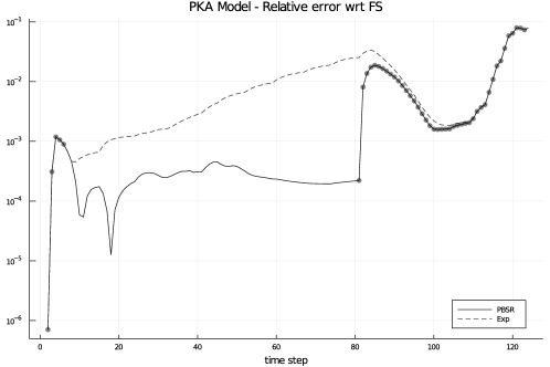
Figure 2: Relative error of the sensitivity matrix, against time step, for the PBSR (solid line) and the Exponential (dashed line) algorithms for the PKA model. The simulations are run over the time span $[0,600]$. The small circles superimposed on the solid line indicate the time steps at which the exponential transition matrix is used instead of the Peano-Baker series approximation.

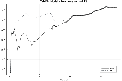
Figure 3: Relative error of the sensitivity matrix, against time step, for the PBSR (solid line) and the Exponential (dashed line) algorithms for the CaMKII model. The simulations are run over the time span $[0,600]$. The small circles superimposed on the solid line indicate the time steps at which the exponential transition matrix is used instead of the Peano-Baker series approximation.

Random linear system

In order to investigate numerically how an increase in the dimensions $n_{x}$ and $n_{p}$ impacts the two algorithms, we implemented a random linear system for which we can choose arbitrary dimensions $n_{x}$; for convenience we set this to be equal to the parameter space dimension $n_{p}$ and denote both with $n$.

The model is obtained by first generating a random matrix $\mathbf{B}$ of dimension $n\times n$ and a random vector $\mathbf{p}$ of length $n$, both with values uniformly distributed in the interval $[0,1]$. Next, we define $\mathbf{A}:=-\mathbf{B}^{T}\mathbf{B}$ and the input vector $\mathbf{u}$ as an $n$ dimensional vector of ones. We then define the corresponding (random) linear system as

$$\dot{\mathbf{x}}(t)=\mathbf{A}\mathbf{x}+\mathbf{p}^{2}+\mathbf{u},$$

which we use to test how the dimension of the system affects the runtime of the three algorithms (PBSR, Exponential and FS).

In this example, the Jacobian is $\nabla_{x}f$ is constant by construction—$\nabla_{x}f\equiv\mathbf{A}$—and the if-statement (45) in Algorithm 2 is always true and there would never be a refinement of the time intervals $[t_{k};t_{k+1}]$, leading to the same output as the Exponential algorithm (in approximately the same computation time). Therefore, to test the approximation based on the Peano-Baker series, we eliminate the if-statement and always apply the Peano-Baker series approximation, including the refinement of the time grid, to approximate the state-transition matrix and compute $\mathbf{S}$.

We performed tests of the three algorithms on this type of random linear system of dimensions $n=5,10,\dots,95,100$. In Figure 4 we show the average runtime (over $10$ iterations) of the FS algorithm (solid line), the PBSR algorithm (dashed line) and Exponential (dotted line). To determine how the runtime scales with the dimension $n$ of the system, we perform regressions on the form $\text{runtime}=a\cdot\text{dimension}^{b}$, using runtime data for each of the three algorithms. The results suggest a runtime of $O(n^{2.1})$ for the Exp algorithm, $O(n^{3.7})$ for the PBSR and $O(n^{4.2})$ for the FS. Therefore, according to this estimate, the PBSR algorithm gives an improvement of approximately $n^{0.5}$ compared to the FS method.

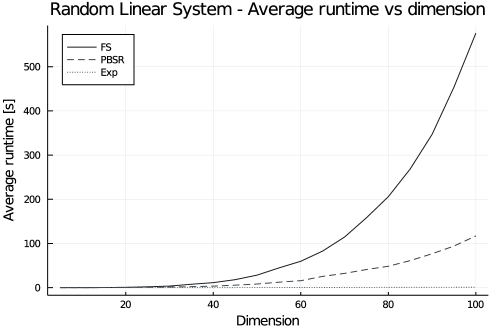
Figure 4: Average running time (over 10 iterations) of the FS (solid line), PBSR (dashed line) and Exponential (dotted line) algorithms applied to random linear systems of dimension $5,10,\dots,100$.

Dynamical system modelling Chua’s circuit

Given the higher efficiency of the Exponential algorithm observed for the random linear systems (see Figure 4), it is natural to ask whether the PBSR algorithm is worth the additional computational effort. The following example shows that it can indeed be the case: consider the three-dimensional dynamical system,

$$\begin{cases}\dot{x}_{1}=p_{1}(x_{2}-x_{1}-f(x)),\\ \dot{x}_{2}=x_{1}-x_{2}+x_{3},\\ \dot{x}_{3}=-p_{2}x_{2},\end{cases}$$

with $f(x)=-8/7x_{1}+4/63x_{1}^{3}$, parameters $p_{1}=7$, $p_{2}=15$, and initial condition $\mathbf{x}_{0}=(0,0,-0.1)^{T}$. This system models Chua’s circuit, an electrical circuit consisting of two capacitors and an inductor, and the choice of parameters and initial condition causes the system to converge to a limit cycle.

In this example, the Jacobian $\nabla_{x}f$ shows high variability within time steps $[t_{k},t_{k+1}]$. The PBSR algorithm (Algorithm 2), because of the refinement of the time intervals, is able to capture these variations, and provides an approximation of the sensitivity matrix $\hat{\mathbf{S}}$ about one order of magnitude more accurate than the Exponential algorithm (Algorithm 3); the results are shown in Figure 5.

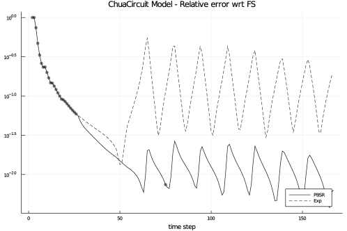
Figure 5: Relative error of the sensitivity matrix, against time step, for the PBSR (solid line) and the Exponential (dashed line) algorithms for the Chua system. The simulations are run over the time span $[0,10]$. The small circles superimposed on the solid line indicate the time steps at which the exponential transition matrix is used instead of the Peano-Baker series approximation.

7 Conclusion and future Work

In this paper we address the problem of computing the sensitivity matrix of parameter-dependent ODE models in high-dimensional settings, where the forward or adjoint methods become too slow for practical purposes. This situation arises in, e.g., uncertainty quantification using Bayesian methods, where there can be a need to compute the sensitivity matrix at a large number of time steps and parameter values, and the parameter space is high-dimensional.

We develop a new method based on the Peano-Baker series from control theory, which is used to derive a representation of the sensitivity matrix $\mathbf{S}$. By truncating the series and applying the trapezoidal rule for the integrals involved we construct an approximation to $\mathbf{S}$ amenable to numerical computation. In addition to the general representation of 2, in Corollary 1 we derive a simplified form in the setting of constant coefficients and forcing term in the ODE for $\mathbf{S}$. This lead to a second numerical method, referred to as the exponential algorithm, which is exact when the system is at equilibrium and a good approximation when the vector field of the ODE system has an almost-constant Jacobian $\nabla_{x}f$. In Section 6 we describe how the two methods can be combined to further speed up the numerical computations while maintaining high accuracy.

A rigorous error analysis shows that, under standard regularity assumptions, the proposed algorithm, based on the Peano-Baker series, admits a global error of order $O(\Delta t_{max}^{2})$. The analysis also shows that the proposed method is optimal in the sense of at what term the Peano-Baker series is truncated. This error analysis is complemented by several numerical experiments. We compare the performance of the different methods to that of the forward sensitivity method for two ODE models from systems biology, a random linear system and a system modelling Chua’s circuit. The results show that both our algorithms produce accurate approximations of the sensitivity matrix with significant speed-up, which seems to increase rapidly with the dimensionality of the problem. In the dynamical system modeling Chua’s circuit, the limit trajectory of the ODE is a limit cycle and thus the Jacobians never becomes (close to) constant. In this example the PBS algorithm produces approximations that have an accuracy one order of magnitude higher than that of the exponential algorithm, which motivates the use of the PBS algorithm for accuracy in general problems. A further motivation comes from the applications in neuroscience that we consider, where ODE models are commonly characterised by time-dependent inputs (e.g. Ca-spike trains). Here the framework is similar to the Chua’s circuit example, where the Jacobians are time-variant, thus the PBS algorithm is expected to be more precise than the Exponential algorithm.

The results of this paper are expected to be beneficial for applications to MCMC methods in systems biology: the speed-up provided by the PBS(R) and Exponential algorithms with respect to forward sensitivity analysis should drastically increase the efficiency of the MCMC methods. As a first test we equipped an implementation of the SMMALA algorithm (in C, CVODES solver) with the near-steady-state sensitivity approximation method to compute the Fisher Information and posterior gradients and compared it to SMMALA with conventional forward sensitivity analysis. The (real) data used for MCMC was obtained at or near the steady-state of the system, so the approximation is justified. The near-steady-state sensitivity approximation allowed the SMMALA algorithm to sample approximately $100$ times faster from the posterior distribution than CVODES’ forward sensitivity analysis. Similar tests on the PBSR algorithm are left for the future.

Future work also includes further investigation of the impact of different implementation aspects of the PBS algorithm—e.g. the switching criteria (based on the Jacobian $\nabla_{x}f$) and the refinement of the time grid of the ODE solver—and properly introducing the method in MCMC sampling. Additional comparisons with existing methods and a better understanding of the methods performance, particularly in large-scale systems, is another important direction.

Funding

The study was supported by Swedish eScience Research Centre (SeRC), EU/Horizon 2020 no. 785907 (HBP SGA2) and no. 945539 (HBP SGA3).

The research of PN was supported in part by the Swedish Research Council (VR-2018-07050) and the Wallenberg AI, Autonomous Systems and Software Program (WASP) funded by the Knut and Alice Wallenberg Foundation.

References

- [1] Michael Baake and Ulrike Schlägel “The Peano-Baker series” In Proceedings of the Steklov Institute of Mathematics 275, 2010 DOI: 10.1134/S0081543811080098
- [2] Alessandro Barp, François-Xavier Briol, Anthony D. Kennedy and Mark Girolami “Geometry and dynamics for Markov chain Monte Carlo” In Annu. Rev. Stat. Appl. 5, 2018, pp. 451–474 DOI: 10.1146/annurev-statistics-031017-100141
- [3] Roger W. Brockett “Finite dimensional linear systems”, Classics in applied mathematics ; 74, 2015
- [4] Dan G. Cacuci “Sensitivity and uncertainty analysis. Vol. I” Theory Chapman & Hall/CRC, Boca Raton, FL, 2003, pp. xviii+285
- [5] Dan G. Cacuci, Mihaela Ionescu-Bujor and Ionel Michael Navon “Sensitivity and uncertainty analysis. Vol. II” Applications to large-scale systems Chapman & Hall/CRC, Boca Raton, FL, 2005, pp. xii+352 DOI: 10.1201/9780203483572
- [6] Jonathan Calver and Wayne Enright “Numerical methods for computing sensitivities for ODEs and DDEs” In Numer. Algorithms 74.4, 2017, pp. 1101–1117 DOI: 10.1007/s11075-016-0188-6
- [7] Yang Cao, Shengtai Li, Linda Petzold and Radu Serban “Adjoint Sensitivity Analysis for Differential-Algebraic Equations: The Adjoint DAE System and Its Numerical Solution” In SIAM Journal on Scientific Computing 24.3, 2003, pp. 1076–1089 DOI: 10.1137/S1064827501380630
- [8] Makis Caracotsios and Warren E. Stewart “Sensitivity analysis of initial value problems with mixed odes and algebraic equations” In Computers & Chemical Engineering 9.4, 1985, pp. 359–365 DOI: https://doi.org/10.1016/0098-1354(85)85014-6
- [9] Timothy W. Church et al. “AKAP79 enables calcineurin to directly suppress protein kinase A activity” In bioRxiv Cold Spring Harbor Laboratory, 2021 DOI: 10.1101/2021.03.14.435320
- [10] O Eriksson et al. “Uncertainty quantification, propagation and characterization by Bayesian analysis combined with global sensitivity analysis applied to dynamical intracellular pathway models” In Bioinformatics 35, 2019, pp. 284–292
- [11] Paul M. Frank “Introduction to system sensitivity theory” Academic Press [Harcourt Brace Jovanovich, Publishers], New York-London, 1978, pp. xiv+386
- [12] Nicolas Garcia Trillos and Daniel Sanz-Alonso “The Bayesian update: variational formulations and gradient flows” In Bayesian Anal. 15.1, 2020, pp. 29–56 DOI: 10.1214/18-BA1137
- [13] Mark Girolami and Ben Calderhead “Riemann manifold Langevin and Hamiltonian Monte Carlo methods” In Journal of the Royal Statistical Society: Series B (Statistical Methodology) 73.2, 2011, pp. 123–214
- [14] David F. Griffiths and Desmond J. Higham “Numerical methods for ordinary differential equations” Initial value problems, Springer Undergraduate Mathematics Series Springer-Verlag London, Ltd., London, 2010, pp. xiv+271 DOI: 10.1007/978-0-85729-148-6
- [15] E. Hairer, S.. Nørsett and G. Wanner “Solving ordinary differential equations. I” Nonstiff problems 8, Springer Series in Computational Mathematics Springer-Verlag, Berlin, 1993, pp. xvi+528
- [16] E. Hairer and G. Wanner “Solving ordinary differential equations. II” Stiff and differential-algebraic problems, Second revised edition, paperback 14, Springer Series in Computational Mathematics Springer-Verlag, Berlin, 2010, pp. xvi+614 DOI: 10.1007/978-3-642-05221-7
- [17] Guri I. Marchuk “Adjoint equations and analysis of complex systems” Translated from the 1992 Russian edition by Guennadi Kontarev and revised by the author 295, Mathematics and its Applications Kluwer Academic Publishers Group, Dordrecht, 1995, pp. x+466 DOI: 10.1007/978-94-017-0621-6
- [18] Guri I. Marchuk, Valeri I. Agoshkov and Victor P. Shutyaev “Adjoint equations and perturbation algorithms in nonlinear problems” CRC Press, Boca Raton, FL, 1996, pp. xii+275
- [19] Anu G. Nair et al. “Chapter Twelve - Modeling Intracellular Signaling Underlying Striatal Function in Health and Disease” In Computational Neuroscience 123, Progress in Molecular Biology and Translational Science Academic Press, 2014, pp. 277–304 DOI: https://doi.org/10.1016/B978-0-12-397897-4.00013-9
- [20] Wilson J Rugh “Linear system theory” Englewood Cliffs, N.J.: Prentice Hall, 1993
- [21] Andrea Saltelli, Stefano Tarantola, Francesca Campolongo and Marco Ratto “Sensitivity analysis in practice” A guide to assessing scientific models John Wiley & Sons, Ltd., Chichester, 2004, pp. xii+219
- [22] Tim Sauer “Numerical analysis” Boston: Pearson/Addison Wesley, 2006