Scalable Spatiotemporally Varying Coefficient modeling with Bayesian Kernelized Tensor Regression

Abstract

As a regression technique in spatial statistics, the spatiotemporally varying coefficient model (STVC) is an important tool for discovering nonstationary and interpretable response-covariate associations over both space and time. However, it is difficult to apply STVC for large-scale spatiotemporal analyses due to its high computational cost. To address this challenge, we summarize the spatiotemporally varying coefficients using a third-order tensor structure and propose to reformulate the spatiotemporally varying coefficient model as a special low-rank tensor regression problem. The low-rank decomposition can effectively model the global patterns of the large data sets with a substantially reduced number of parameters. To further incorporate the local spatiotemporal dependencies, we use Gaussian process (GP) priors on the spatial and temporal factor matrices. We refer to the overall framework as Bayesian Kernelized Tensor Regression (BKTR). For model inference, we develop an efficient Markov chain Monte Carlo (MCMC) algorithm, which uses Gibbs sampling to update factor matrices and slice sampling to update kernel hyperparameters. We conduct extensive experiments on both synthetic and real-world data sets, and our results confirm the superior performance and efficiency of BKTR for model estimation and parameter inference.

Keywords: Gaussian process; Tensor regression; Bayesian framework; Multivariate spatiotemporal processes; Spatiotemporal modeling

1 Introduction

Local spatial regression aims to characterize the nonstationary and heterogeneous associations between the response variable and corresponding covariates observed in a spatial domain (Banerjee et al., 2014; Cressie & Wikle, 2015). This is achieved by assuming that the regression coefficients vary locally over space. Local spatial regression offers enhanced interpretability of complex relationships, and has become an important technique in many fields, such as geography, ecology, economics, environment, public health and climate science, to name but a few. In general, a local spatial regression model for a scalar response $y$ can be written as:

$$y(\boldsymbol{s})=\boldsymbol{x}(\boldsymbol{s})^{\top}\boldsymbol{\beta}(\boldsymbol{s})+\epsilon(\boldsymbol{s}),$$ (1)

where $\boldsymbol{s}$ is the index (e.g., longitude and latitude) for a spatial location, $\boldsymbol{x}(\boldsymbol{s})\in\mathbb{R}^{P}$ and $\boldsymbol{\beta}(\boldsymbol{s})\in\mathbb{R}^{P}$ are the covariate vector and the regression coefficients at location $\boldsymbol{s}$, respectively, and $\epsilon(\boldsymbol{s})\sim\text{i.i.d.}\,\mathcal{N}(0,\tau^{-1})$ is a white noise process with precision $\tau$.

There are two common methods for local spatial regression analysis—the Bayesian spatially varying coefficient model (SVC) (Gelfand et al., 2003) and the geographically weighted regression (GWR) (Fotheringham et al., 2003). SVC is a Bayesian hierarchical model where regression coefficients are modelled using Gaussian processes (GP) with a kernel function to be learned (Rasmussen & Williams, 2006). For a collection of $M$ observed locations, the original SVC developed by Gelfand et al. (2003) imposes a prior such that $\text{vec}(\boldsymbol{\beta}_{\text{mat}}^{\top})\sim\mathcal{N}(\boldsymbol{1}_{M\times 1}\otimes\boldsymbol{\mu}_{\beta},\boldsymbol{K}_{s}\otimes\boldsymbol{\Lambda}^{-1})$, where $\boldsymbol{\beta}_{\text{mat}}$ is a $M\times P$ matrix of all coefficients, $\text{vec}(\boldsymbol{X})$ denotes vectorization by stacking all columns in $\boldsymbol{X}$ as a vector, $\boldsymbol{\mu}_{\beta}$ represents the overall regression coefficient vector used to constructed the mean, $\boldsymbol{K}_{s}$ is a $M\times M$ spatial correlation matrix, $\boldsymbol{\Lambda}$ is a $P\times P$ precision matrix for covariates, and $\otimes$ denotes the Kronecker product. In this paper, for simplicity, we use a zero-mean GP to specify $\boldsymbol{\beta}$, and the global effect of covariates can be learned (or removed) through a linear regression term as in Gelfand et al. (2003). Also, setting $\boldsymbol{K}_{s}$ as a correlation matrix simplifies the covariance specification, since the variance can be captured by scaling $\boldsymbol{\Lambda}^{-1}$. This formulation is equivalent to having a matrix normal distribution $\boldsymbol{\beta}_{\text{mat}}\sim\mathcal{MN}_{M\times P}\left(\boldsymbol{0},\boldsymbol{K}_{s},\boldsymbol{\Lambda}^{-1}\right)$. GWR was developed independently using a local weighted regression approach, in which a bandwidth parameter is used to calculate the weights (based on a weight function) for different observations, with closer observations carrying larger weights. In practice, the bandwidth parameter is either pre-specified based on domain knowledge or tuned through cross-validation. However, it has been shown in the literature that the estimation results of GWR are highly sensitive to the selection of the bandwidth parameter (e.g., Finley, 2011). Compared with GWR, the Bayesian hierarchical framework of SVC provides more robust results and allows us to learn the hyperparameters of the spatial kernel $\boldsymbol{K}_{s}$, which is critical to understanding the underlying characteristics of the spatial processes. In addition, by using Markov chain Monte Carlo (MCMC), we can not only explore the posterior distribution of the kernel hyperparameters and regression coefficients, but also perform out-of-sample prediction.

The formulation in Eq. (1) can be easily extended to local spatiotemporal regression to further characterize the temporal variation of coefficients. For a response matrix $\boldsymbol{Y}\in\mathbb{R}^{M\times N}$ observed from a set of locations $S=\{\boldsymbol{s}_{1},\cdots,\boldsymbol{s}_{M}\}$ over a set of time points $T=\{t_{1},\cdots,t_{N}\}$, the local spatiotemporal regression model defined on the Cartesian product $S\times T=\left\{\left(\boldsymbol{s}_{m},t_{n}\right):m=1,\ldots,M,\ n=1,\ldots,N\right\}$ can be formulated as:

$$y\left(\boldsymbol{s}_{m},t_{n}\right)=\boldsymbol{x}\left(\boldsymbol{s}_{m},t_{n}\right)^{\top}\boldsymbol{\beta}\left(\boldsymbol{s}_{m},t_{n}\right)+\epsilon\left(\boldsymbol{s}_{m},t_{n}\right),$$ (2)

where we use $m=1,\cdots,M$ and $n=1,\cdots,N$ to index rows (i.e., location) and columns (i.e., time point), respectively, $y\left(\boldsymbol{s}_{m},t_{n}\right)$ is the $(m,n)$th element in $\boldsymbol{Y}$, and $\boldsymbol{x}\left(\boldsymbol{s}_{m},t_{n}\right)$ and $\boldsymbol{\beta}\left(\boldsymbol{s}_{m},t_{n}\right)$ are the covariate vector and coefficient vector at location $\boldsymbol{s}_{m}$ and time $t_{n}$, respectively. Based on this formulation, Huang et al. (2010) extended GWR to geographically and temporally weighted regression (GTWR) by introducing more parameters to quantify spatiotemporal weights in the local weighted regression. For SVC, Gelfand et al. (2003) suggested using a separable kernel structure to build a spatiotemporally varying coefficient model (STVC), which assumes that $\left[\boldsymbol{\beta}\left(\boldsymbol{s}_{1},t_{1}\right);\cdots;\boldsymbol{\beta}\left(\boldsymbol{s}_{M},t_{1}\right);\boldsymbol{\beta}\left(\boldsymbol{s}_{1},t_{2}\right);\cdots;\boldsymbol{\beta}\left(\boldsymbol{s}_{M},t_{N}\right)\right]\sim\mathcal{N}(\boldsymbol{0},\boldsymbol{K}_{t}\otimes\boldsymbol{K}_{s}\otimes\boldsymbol{\Lambda}^{-1})$, where $\boldsymbol{K}_{t}$ is a $N\times N$ kernel matrix defining the correlation structure for the $N$ time points. Note that with this GP formulation, it is not necessary for the $N$ time points to be uniformly distributed. If we parameterize the regression coefficients in Eq. (2) as a third-order tensor $\boldsymbol{\mathcal{B}}\in\mathbb{R}^{M\times N\times P}$ with mode-3 fiber $\boldsymbol{\mathcal{B}}(m,n,:)=\boldsymbol{\beta}\left(\boldsymbol{s}_{m},t_{n}\right)$, the above specification is equivalent to having a tensor normal distribution $\boldsymbol{\cal{B}}\sim\mathcal{TN}_{M\times N\times P}\left(\boldsymbol{0},\boldsymbol{K}_{s},\boldsymbol{K}_{t},\boldsymbol{\Lambda}^{-1}\right)$. However, despite the elegant separable kernel-based formulation in STVC, the model is rarely used in real-world practice mainly due to the high computational cost. For example, for a fully observed matrix $\boldsymbol{Y}$ with corresponding spatiotemporal covariates, updating kernel hyperparameters and the coefficients $\boldsymbol{\beta}$ in each MCMC iteration requires time complexity of $\mathcal{O}\left(M^{3}N^{3}\right)$ and $\mathcal{O}\left(M^{3}N^{3}P^{3}\right)$, respectively.

In this paper, we provide an alternative estimation strategy—Bayesian Kernelized Tensor Regression (BKTR)—to perform Bayesian spatiotemporal regression analysis on large-scale data sets. Inspired by the idea of reduced rank regression and tensor regression (e.g., Izenman, 1975; Zhou et al., 2013; Bahadori et al., 2014; Guhaniyogi et al., 2017), we use low-rank tensor factorization to encode the dependencies among the three dimensions in $\boldsymbol{\mathcal{B}}$ with only a few latent factors. To further incorporate local spatial and temporal dependencies, we use GP priors on the spatial and temporal factor vectors following Luttinen & Ilin (2009), thus translating the default tensor factorization into a kernelized factorization model. With a specified tensor rank $R$, the time complexity becomes $\mathcal{O}\left(R^{3}\left(M^{3}+N^{3}+P^{3}\right)\right)$, which is substantially reduced compared with the default STVC formulation. In addition to the spatial and temporal framework, we also consider in this paper the case where a proportion of response matrix $\boldsymbol{Y}$ can be unobserved or corrupted, given observed values of the covariates $\boldsymbol{X}$. Such a scenario is very common in many real-world applications, such as traffic state data collected from emerging crowdsourcing and moving sensing systems (e.g., Google Waze) for example, where observations are inherently sparse in space and time. We show that the underlying Bayesian tensor decomposition structure allows us to effectively estimate both the model coefficients and the unobserved outcomes even when the missing rate of $\boldsymbol{Y}$ is high. We conduct numerical experiments on both synthetic and real-world data sets, and our results confirm the promising performance of BKTR.

2 Related Work

The key computational challenge in SVC/STVC is how to efficiently and effectively learn a multivariate spatial/spatiotemporal process (i.e., $\boldsymbol{\beta}_{\text{mat}}$ in Eq. (1) and the third-order spatiotemporal tensor $\boldsymbol{\cal{B}}$ in Eq. (2)). For a general multivariate spatial process which is fully observed on the Cartersian product with white noise, a popular approach is to use separable covariance specification on which one can leverage property of Kronecker products to substantially reduce the computational cost (Saatçi, 2012; Wilson et al., 2014). However, for SVC, we cannot benefit from the Kronecker property directly since the data $\boldsymbol{y}$ is obtained through a linear transformation of $\boldsymbol{\beta}_{\text{mat}}$. In this case, computing the inverse of an $MP\times MP$ matrix becomes inevitable when sampling those space-varying coefficients. Existing frameworks for SVC essentially adopt a two-step approach (Gelfand et al., 2003; Finley & Banerjee, 2020): (1) update only kernel hyperparameters and $\boldsymbol{\mu}$ by marginalizing $\boldsymbol{\beta}$ with cost $\mathcal{O}\left(M^{3}\right)$; and (2) after burn-in, use composition sampling on of the obtained MCMC samples to obtain samples for $\boldsymbol{\beta}$ with cost $\mathcal{O}\left(M^{3}P^{3}\right)$. For STVC, the corresponding costs in the two steps are $\mathcal{O}\left(M^{3}N^{3}\right)$ and $\mathcal{O}\left(M^{3}N^{3}P^{3}\right)$, respectively. The high computational cost in step (2) is the key issue that limits the application of SVC/STVC in practice.

Our work follows a different approach. Instead of modeling $\boldsymbol{\beta}$ directly using a GP, we parameterize the third-order tensor $\boldsymbol{\cal{B}}$ for STVC using a probabilistic low-rank tensor decomposition (Kolda & Bader, 2009). The idea is inspired by recent studies on low-rank tensor regression/learning (see e.g., Zhou et al., 2013; Bahadori et al., 2014; Rabusseau & Kadri, 2016; Yu & Liu, 2016; Guhaniyogi et al., 2017; Yu et al., 2018). The low-rank assumption not only preserves the global patterns and higher-order dependencies in the variable, but also greatly reduces the number of parameters. In fact, without considering the spatiotemporal indices, we can formulate Eq. (2) as a scalar tensor regression problem (Guhaniyogi et al., 2017) by reconstructing each $\boldsymbol{x}(\boldsymbol{s}_{m},t_{n})$ as a sparse covariate tensor of the same size as $\boldsymbol{\cal{B}}$. However, for spatiotemporal data, the low-rank assumption alone cannot fully characterize the strong local spatial and temporal consistency. To better encode local spatial and temporal consistency, existing studies have introduced graph Laplacian regularization in defining the loss function (e.g., Bahadori et al., 2014; Rao et al., 2015). Nevertheless, this approach also introduces more parameters (e.g., those used to define distance/similarity function and weights in the loss function) and it has limited power in modeling complex spatial and temporal processes. The most relevant work is a Gaussian process factor analysis model (Luttinen & Ilin, 2009) developed for a completely different problem—spatiotemporal matrix completion, in which different GP priors are assumed on the spatial and temporal factors and the whole model is learned through variational Bayesian inference. Lei et al. (2022) presents an MCMC scheme for this model, in which slice sampling is used to update kernel hyperparameters and Gibbs sampling is used to update factor matrices. We follow a similar idea as in Luttinen & Ilin (2009) and Lei et al. (2022) to parameterize the coefficients $\boldsymbol{\beta}$ and develop MCMC algorithms for model inference.

3 Bayesian Kernelized Tensor Regression

3.1 Notations

Throughout this paper, we use lowercase letters to denote scalars, e.g., $x$, boldface lowercase letters to denote vectors, e.g., $\boldsymbol{x}\in\mathbb{R}^{M}$, and boldface uppercase letters to denote matrices, e.g., $\boldsymbol{X}\in\mathbb{R}^{M\times N}$. The $\ell_{2}$-norm of $\boldsymbol{x}$ is defined as $\|\boldsymbol{x}\|_{2}=\sqrt{\sum_{m}x_{m}^{2}}$. For a matrix $\boldsymbol{X}\in\mathbb{R}^{M\times N}$, we denote its $(m,n)$th entry by $x_{m,n}$. We use $\boldsymbol{I}_{N}$ to denote an identity matrix of size $N\times N$. Given two matrices $\boldsymbol{A}\in\mathbb{R}^{M\times N}$ and $\boldsymbol{B}\in\mathbb{R}^{P\times Q}$, the Kronecker product is defined as $\boldsymbol{A}\otimes\boldsymbol{B}=\footnotesize{\begin{bmatrix}a_{1,1}\boldsymbol{B}&\cdots&a_{1,N}\boldsymbol{B}\\ \vdots&\ddots&\vdots\\ a_{M,1}\boldsymbol{B}&\cdots&a_{M,N}\boldsymbol{B}\end{bmatrix}}\in\mathbb{R}^{MP\times NQ}$. If $\boldsymbol{A}=[\boldsymbol{a}_{1},\cdots,\boldsymbol{a}_{N}]$ and $\boldsymbol{B}=[\boldsymbol{b}_{1},\cdots,\boldsymbol{b}_{Q}]$ have the same number of columns, i.e., $N=Q$, then the Khatri-Rao product is defined as the column-wise Kronecker product $\boldsymbol{A}\odot\boldsymbol{B}=[\boldsymbol{a}_{1}\otimes\boldsymbol{b}_{1},\cdots,\boldsymbol{a}_{N}\otimes\boldsymbol{b}_{N}]\in\mathbb{R}^{MP\times N}$. The vectorization $\operatorname{vec}(\boldsymbol{X})$ stacks all column vectors in $\boldsymbol{X}$ as a single vector. Following the tensor notation in Kolda & Bader (2009), we denote a third-order tensor by $\boldsymbol{\mathcal{X}}\in\mathbb{R}^{M\times N\times P}$ and its mode-$k$ $(k=\text{1},\text{2},\text{3})$ unfolding by $\boldsymbol{X}_{(k)}$, which maps a tensor into a matrix. The mode-3 fibers and frontal slices of $\boldsymbol{\mathcal{X}}$ are denoted by $\boldsymbol{\mathcal{X}}(m,n,:)\in\mathbb{R}^{p}$ and $\boldsymbol{\mathcal{X}}(:,:,p)\in\mathbb{R}^{M\times N}$, respectively. Finally, we use $\operatorname{ones}(M,N)$ and $\boldsymbol{1}_{M}\in\mathbb{R}^{M}$ to represent a $M\times N$ matrix and a length $M$ column vector of ones, respectively.

3.2 Tensor CP Decomposition

For a third-order tensor $\boldsymbol{\mathcal{A}}\in\mathbb{R}^{M\times N\times P}$, the CANDECOMP/PARAFAC (CP) decomposition factorizes $\boldsymbol{\mathcal{A}}$ into a sum of rank-one tensors (Kolda & Bader, 2009):

$$\boldsymbol{\mathcal{A}}=\sum_{r=1}^{R}\boldsymbol{u}_{r}\circ\boldsymbol{v}_{r}\circ\boldsymbol{w}_{r},$$ (3)

where $R$ is the CP rank, $\circ$ represents the outer product, $\boldsymbol{u}_{r}\in\mathbb{R}^{M}$, $\boldsymbol{v}_{r}\in\mathbb{R}^{N}$, and $\boldsymbol{w}_{r}\in\mathbb{R}^{P}$ for $r=1,\cdots,R$. The factor matrices that combine the vectors from the rank-one components are denoted by $\boldsymbol{U}=[\boldsymbol{u}_{1},\cdots,\boldsymbol{u}_{R}]\in\mathbb{R}^{M\times R}$, $\boldsymbol{V}\in\mathbb{R}^{N\times R}$, and $\boldsymbol{W}\in\mathbb{R}^{P\times R}$, respectively. We can write Eq. (3) in the following matricized form:

$$\begin{split}\boldsymbol{A}_{(1)}=\boldsymbol{U}\left(\boldsymbol{W}\odot\boldsymbol{V}\right)^{\top},~{}\boldsymbol{A}_{(2)}=\boldsymbol{V}\left(\boldsymbol{W}\odot\boldsymbol{U}\right)^{\top},~{}\boldsymbol{A}_{(3)}=\boldsymbol{W}\left(\boldsymbol{V}\odot\boldsymbol{U}\right)^{\top},\end{split}$$ (4)

which relates the mode-$k$ unfolding of a tensor to its polyadic decomposition.

3.3 Model Specification

Let $\boldsymbol{\mathcal{X}}$ be an $M\times N\times P$ tensor, of which the $(m,n)$th mode-3 fiber is the covariate vector at location $\boldsymbol{s}_{m}$ and time $t_{n}$, i.e., $\boldsymbol{\mathcal{X}}{(m,n,:)}=\boldsymbol{x}\left(\boldsymbol{s}_{m},t_{n}\right)$. For example, in the application of spatiotemporal modeling on bike-sharing demand that we illustrate later (see Section 5), the response matrix $\boldsymbol{Y}\in\mathbb{R}^{M\times N}$ is a matrix of daily departure trips for $M$ bike stations over $N$ days, and the tensor variable $\boldsymbol{\mathcal{X}}\in\mathbb{R}^{M\times N\times P}$ represents a set of $P$ spatiotemporal covariates for the corresponding locations and time. Using $\boldsymbol{y}\in\mathbb{R}^{MN}$ to denote $\operatorname{vec}(\boldsymbol{Y})$, Eq. (2) can be formulated as:

$$\boldsymbol{y}=\left(\boldsymbol{I}_{MN}\odot\boldsymbol{X}_{(3)}\right)^{\top}\operatorname{vec}\left(\boldsymbol{B}_{(3)}\right)+\boldsymbol{\epsilon},$$ (5)

where $\boldsymbol{X}_{(3)}$ and $\boldsymbol{B}_{(3)}$ are the unfoldings of $\boldsymbol{\mathcal{X}}$ and $\boldsymbol{\mathcal{B}}$, respectively, the Khatri-Rao product $\left(\boldsymbol{I}_{MN}\odot\boldsymbol{X}_{(3)}\right)^{\top}$ is a $MN\times MNP$ block diagonal matrix, and $\boldsymbol{\epsilon}\sim\mathcal{N}(\boldsymbol{0},\tau^{-1}\boldsymbol{I}_{MN})$. Assuming that $\boldsymbol{\mathcal{B}}=\sum_{r=1}^{R}\boldsymbol{u}_{r}\circ\boldsymbol{v}_{r}\circ\boldsymbol{w}_{r}$ admits a CP decomposition with rank $R\ll\min\{M,N\}$, we can rewrite Eq. (5) as:

$$\boldsymbol{y}=\tilde{\boldsymbol{X}}\operatorname{vec}\left(\boldsymbol{W}(\boldsymbol{V}\odot\boldsymbol{U})^{\top}\right)+\boldsymbol{\epsilon},$$ (6)

where $\tilde{\boldsymbol{X}}=\left(\boldsymbol{I}_{MN}\odot\boldsymbol{X}_{(3)}\right)^{\top}$ denotes the expanded covariate matrix. The number of parameters in (6) is $R(M+N+P)$, which is substantially smaller than $MNP$ in (5).

Local spatial and temporal processes are critical to the modeling of spatiotemporal data. However, as mentioned, the low-rank assumption alone cannot encode such local dependencies. To address this issue, we assume specific GP priors on $\boldsymbol{U}$ and $\boldsymbol{V}$, respectively, following the GP factor analysis strategy (Luttinen & Ilin, 2009), and then develop a fully Bayesian approach to estimate the model in Eq. (6). Figure 1 illustrates the proposed framework, which is referred to as Bayesian Kernelized Tensor Regression (BKTR) in the remainder of this paper. The graphical model of BKTR is shown in Figure 2.

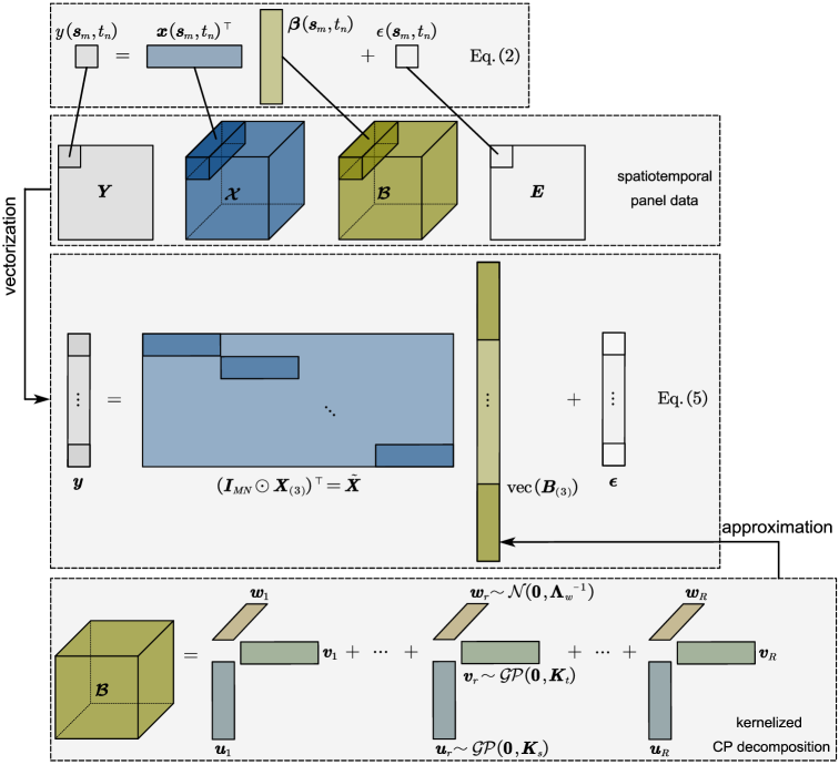
Figure 1: Illustration of the proposed BKTR framework.

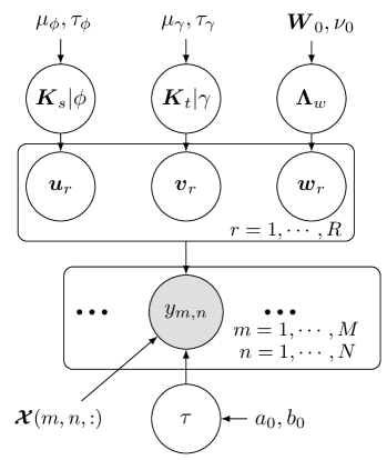
Figure 2: Graphical model of BKTR.

As mentioned in the introduction, in real-world applications the dependent data is often partially observed on a set $\Omega$ of observation indices, with $|\Omega|<MN$. This means that we only observe a subset of entries $y_{m,n}$, for $\forall(s_{m},t_{m})\in\Omega$. We denote by $\boldsymbol{D}\in\mathbb{R}^{M\times N}$ a binary indicator matrix with $d_{m,n}=1$ if $(m,n)\in\Omega$ and $d_{m,n}=0$ otherwise, and denote by $\boldsymbol{O}$ a binary matrix of $|\Omega|\times MN$ formed by removing the rows corresponding to the zero values in $\operatorname{vec}(\boldsymbol{D})$ from a $MN\times MN$ identity matrix. The vector of observed data can be obtained by $\boldsymbol{y}_{\Omega}=\boldsymbol{O}\boldsymbol{y}$. Therefore, we have:

$$\boldsymbol{y}_{\Omega}\sim\mathcal{N}\left(\boldsymbol{O}\left(\tilde{\boldsymbol{X}}\operatorname{vec}\left(\boldsymbol{W}(\boldsymbol{V}\odot\boldsymbol{U})^{\top}\right)\right),\tau^{-1}\boldsymbol{I}_{|\Omega|}\right).$$ (7)

For spatial and temporal factor matrices $\boldsymbol{U}$ and $\boldsymbol{V}$, we use identical GP priors on the component vectors:

$$\boldsymbol{u}_{r} \sim\mathcal{GP}\left(\boldsymbol{0},\boldsymbol{K}_{s}\right),~{}r=1,\cdots,R,$$ (8)

$$\boldsymbol{v}_{r} \sim\mathcal{GP}\left(\boldsymbol{0},\boldsymbol{K}_{t}\right),~{}r=1,\cdots,R,$$

where $\boldsymbol{K}_{s}\in\mathbb{R}^{M\times M}$ and $\boldsymbol{K}_{t}\in\mathbb{R}^{N\times N}$ are the spatial and temporal covariance matrices built from two valid kernel functions $k_{s}(\boldsymbol{s}_{m},\boldsymbol{s}_{m^{\prime}};\phi)$ and $k_{t}(t_{n},t_{n^{\prime}};\gamma)$, respectively, with $\phi$ and $\gamma$ being kernel length-scale hyperparameters. Note that we also restrict $\boldsymbol{K}_{s}$ and $\boldsymbol{K}_{t}$ to being correlation matrices by setting the variance to one, and we capture the variance through $\boldsymbol{W}$. We reparameterize the kernel hyperparameters as log-transformed variables to ensure their positivity and assume normal priors on them, i.e., $\log(\phi)\sim\mathcal{N}(\mu_{\phi},\tau_{\phi}^{-1}),~{}\log(\gamma)\sim\mathcal{N}(\mu_{\gamma},\tau_{\gamma}^{-1})$. For the factor matrix $\boldsymbol{W}$, we assume all columns follow an identical zero-mean Gaussian distribution with a conjugate Wishart prior on the precision matrix:

$$\boldsymbol{w}_{r} \sim\mathcal{N}\left(\boldsymbol{0},\boldsymbol{\Lambda}_{w}^{-1}\right),~{}r=1,\cdots,R,$$ (9)

$$\boldsymbol{\Lambda}_{w} \sim\mathcal{W}\left(\boldsymbol{\Psi}_{0},\nu_{0}\right),$$

where $\boldsymbol{\Psi}_{0}$ is a $P\times P$ positive-definite scale matrix and $\nu_{0}>P-1$ denotes the degrees of freedom. Finally, we suppose a conjugate Gamma prior $\tau\sim\text{Gamma}(a_{0},b_{0})$ on the noise precision $\tau$ defined in Eq. (7).

3.4 Model Inference

We use Gibbs sampling to estimate the model parameters, including coefficient factors $\{\boldsymbol{U},\boldsymbol{V},\boldsymbol{W}\}$, the precision $\tau$, and the precision matrix $\boldsymbol{\Lambda}_{w}$. For the kernel hyperparameters $\{\phi,\gamma\}$ whose conditional distributions are not easy to sample from, we use the slice sampler.

3.4.1 Sampling the coefficient factor matrices $\{\boldsymbol{U},\boldsymbol{V},\boldsymbol{W}\}$

Sampling the factor matrices can be considered as a Bayesian linear regression problem. Taking $\boldsymbol{W}$ as an example, we can rewrite Eq. (7) as:

$$\boldsymbol{y}_{\Omega}\sim\mathcal{N}\left(\boldsymbol{O}\left(\tilde{\boldsymbol{X}}\left((\boldsymbol{V}\odot\boldsymbol{U})\otimes\boldsymbol{I}_{P}\right)\operatorname{vec}(\boldsymbol{W})\right),\tau^{-1}\boldsymbol{I}_{|\Omega|}\right),$$ (10)

where $\boldsymbol{U},\boldsymbol{V}$ are known and $\operatorname{vec}(\boldsymbol{W})$ is the coefficient to estimate. Considering that the priors of each component vector $\boldsymbol{w}_{r}$ are independent and identical, the prior distribution over the whole vectorized $\boldsymbol{W}$ becomes $\operatorname{vec}(\boldsymbol{W})\sim\mathcal{N}(\boldsymbol{0},\boldsymbol{I}_{R}\otimes\boldsymbol{\Lambda}_{w}^{-1})$. Since both likelihood and prior of $\operatorname{vec}(\boldsymbol{W})$ follow Gaussian distributions, its posterior is also Gaussian with mean $\boldsymbol{\mu}_{W}^{*}$ and precision $\boldsymbol{\Lambda}_{W}^{*}$ such as:

$$\boldsymbol{\Lambda}_{W}^{*} =\tau\boldsymbol{H}_{W}^{\top}\boldsymbol{H}_{W}+\boldsymbol{\Lambda}_{W},\ \ \boldsymbol{\Lambda}_{W}=\boldsymbol{I}_{R}\otimes\boldsymbol{\Lambda}_{w},$$

$$\boldsymbol{\mu}_{W}^{*} =\tau(\boldsymbol{\Lambda}_{W}^{*})^{-1}\boldsymbol{H}_{W}^{\top}\boldsymbol{y}_{\Omega},$$

$$\boldsymbol{H}_{W} =\boldsymbol{O}\left(\tilde{\boldsymbol{X}}\left((\boldsymbol{V}\odot\boldsymbol{U})\otimes\boldsymbol{I}_{P}\right)\right).$$

The posterior distributions of $\boldsymbol{U}$ and $\boldsymbol{V}$ can be obtained similarly using different tensor unfoldings. In order to sample $\boldsymbol{U}$, we use the mode-1 unfolding in Eq. (4) and reconstruct the regression model with $\operatorname{vec}(\boldsymbol{U})$ as coefficients:

$$\boldsymbol{y}_{\Omega}=\boldsymbol{O}\left(\tilde{\boldsymbol{X}}_{U}\left((\boldsymbol{W}\odot\boldsymbol{V})\otimes\boldsymbol{I}_{M}\right)\operatorname{vec}(\boldsymbol{U})\right)+\boldsymbol{\epsilon}_{\Omega},$$ (11)

where $\tilde{\boldsymbol{X}}_{U}=\left(\boldsymbol{X}_{(3)}\odot\boldsymbol{I}_{MN}\right)^{\top}\in\mathbb{R}^{MN\times MNP}$ and $\boldsymbol{\epsilon}_{\Omega}\sim\mathcal{N}\left(\boldsymbol{0},\tau^{-1}\boldsymbol{I}_{|\Omega|}\right)$. Thus, the posterior of $\operatorname{vec}(\boldsymbol{U})$ has a closed form—a Gaussian distribution with mean $\boldsymbol{\mu}_{U}^{*}$ and precision $\boldsymbol{\Lambda}_{U}^{*}$, where

$$\boldsymbol{\Lambda}_{U}^{*} =\tau\boldsymbol{H}_{U}^{\top}\boldsymbol{H}_{U}+\boldsymbol{K}_{U}^{-1},\boldsymbol{K}_{U}=\boldsymbol{I}_{R}\otimes\boldsymbol{K}_{s},$$

$$\boldsymbol{\mu}_{U}^{*} =\tau(\boldsymbol{\Lambda}_{U}^{*})^{-1}\boldsymbol{H}_{U}^{\top}\boldsymbol{y}_{\Omega},$$

$$\boldsymbol{H}_{U} =\boldsymbol{O}\left(\tilde{\boldsymbol{X}}_{U}\left((\boldsymbol{W}\odot\boldsymbol{V})\otimes\boldsymbol{I}_{M}\right)\right).$$

The posterior for $\operatorname{vec}(\boldsymbol{V})$ can be obtained by applying the mode-2 tensor unfolding. It should be noted that the above derivation provides the posterior for the whole factor matrix, i.e., $\left\{\operatorname{vec}(\boldsymbol{U}),\operatorname{vec}(\boldsymbol{V}),\operatorname{vec}(\boldsymbol{W})\right\}$. We can further reduce the computing cost by sampling $\left\{\boldsymbol{u}_{r},\boldsymbol{v}_{r},\boldsymbol{w}_{r}\right\}$ one by one for $r=1,\cdots,R$ as in Luttinen & Ilin (2009). In this case, the time complexity in learning these factor matrices can be further reduced to $\mathcal{O}(R(M^{3}+N^{3}+P^{3}))$ at the cost of slow/poor mixing.

3.4.2 Sampling kernel hyperparameters $\{\phi,\gamma\}$

As shown in Figure 2, sampling kernel hyperparameters conditional on the factor matrices should be straightforward through the Metropolis-Hastings algorithm. However, in practice, conditioning on the latent variables $\{\boldsymbol{U},\boldsymbol{V}\}$ in such hierarchical GP models usually induces sharply peaked posteriors over $\{\phi,\gamma\}$, making the Markov chains mix slowly and resulting in poor updates (Murray & Adams, 2010). To address this issue, we integrate out the latent factors from the model to get the marginal likelihood, and sample $\phi$ and $\gamma$ from their marginal posterior distributions based on the slice sampling approach (Neal, 2003).

Let’s consider for example the hyperparameter of $\boldsymbol{K}_{s}$, i.e., $\phi$. As $\operatorname{vec}(\boldsymbol{U})\sim\mathcal{N}(\boldsymbol{0},\boldsymbol{K}_{U})$ with $\boldsymbol{K}_{U}=\boldsymbol{I}_{R}\otimes\boldsymbol{K}_{s}$, we integrate over $\operatorname{vec}(\boldsymbol{U})$ in Eq. (11) and obtain:

$$\log{p\left(\boldsymbol{y}_{\Omega}\;\middle|\;\phi,\boldsymbol{V},\boldsymbol{W},\tau,\boldsymbol{\mathcal{X}}\right)}=-\frac{1}{2}\boldsymbol{y}_{\Omega}^{\top}\boldsymbol{K}_{\left.\boldsymbol{y}\right|\phi}^{-1}\boldsymbol{y}_{\Omega}-\frac{1}{2}\log{\left|\boldsymbol{K}_{\left.\boldsymbol{y}\right|\phi}\right|}-\frac{|\Omega|}{2}\log{2\pi},$$ (12)

where $\boldsymbol{K}_{\left.\boldsymbol{y}\right|\phi}=\boldsymbol{H}_{U}\boldsymbol{K}_{U}\boldsymbol{H}_{U}^{\top}+\tau^{-1}\boldsymbol{I}_{|\Omega|}$ and $\boldsymbol{H}_{U}=\boldsymbol{O}\left(\tilde{\boldsymbol{X}}_{U}\left((\boldsymbol{W}\odot\boldsymbol{V})\otimes\boldsymbol{I}_{M}\right)\right)\in\mathbb{R}^{|\Omega|\times MR}$. The marginal posterior of $\phi$ becomes:

$$\log{p\left(\phi\;\middle|\;\boldsymbol{y}_{\Omega},\boldsymbol{V},\boldsymbol{W},\tau,\boldsymbol{\mathcal{X}}\right)}\propto \log{p(\phi)}-\frac{1}{2}\boldsymbol{y}_{\Omega}^{\top}\boldsymbol{K}_{\left.\boldsymbol{y}\right|\phi}^{-1}\boldsymbol{y}_{\Omega}-\frac{1}{2}\log{\left|\boldsymbol{K}_{\left.\boldsymbol{y}\right|\phi}\right|}$$ (13)

$$\propto \log{p(\phi)}+\frac{1}{2}\tau^{2}\boldsymbol{y}_{\Omega}^{\top}\boldsymbol{H}_{U}\left(\boldsymbol{I}_{R}\otimes\boldsymbol{K}_{s}^{-1}+\tau\boldsymbol{H}_{U}^{\top}\boldsymbol{H}_{U}\right)^{-1}\boldsymbol{H}_{U}^{\top}\boldsymbol{y}_{\Omega}$$

$$-\frac{1}{2}\log{\left|\boldsymbol{I}_{R}\otimes\boldsymbol{K}_{s}^{-1}+\tau\boldsymbol{H}_{U}^{\top}\boldsymbol{H}_{U}\right|}-\frac{R}{2}\log{\left|\boldsymbol{K}_{s}\right|},$$

where we compute $\boldsymbol{y}_{\Omega}^{\top}\boldsymbol{K}_{\left.\boldsymbol{y}\right|\phi}^{-1}\boldsymbol{y}_{\Omega}$ based on the Woodbury matrix identity, and use the matrix determinant lemma to compute $\log{\left|\boldsymbol{K}_{\left.\boldsymbol{y}\right|\phi}\right|}$. The detailed derivation is given in Appendix A. The slice sampling approach is robust to the selection of the sampling scale and easy to implement. Sampling $\gamma$ can be achieved in a similar way. Note that, as mentioned, the sampling is performed on the log-transformed variables to avoid numerical issues. The detailed sampling process for kernel hyperparameters is provided in Appendix B. We can also introduce different kernel functions (or the same kernel function with different hyperparameters) for each factor vector $\boldsymbol{u}_{r}$ and $\boldsymbol{v}_{r}$ as in Luttinen & Ilin (2009). In such a case, the marginal posterior of the kernel hyperparameters can be derived in a similar way as in Eq. (13).

3.4.3 Sampling $\boldsymbol{\Lambda}_{w}$

Given the conjugate Wishart prior, the posterior distribution of $\boldsymbol{\Lambda}_{w}$ is $\left.\boldsymbol{\Lambda}_{w}\right|\boldsymbol{W},\boldsymbol{\Psi}_{0},\nu_{0}\sim\mathcal{W}\left(\boldsymbol{\Psi}^{*},\nu^{*}\right)$, where $[\boldsymbol{\Psi}^{*}]^{-1}=\boldsymbol{W}\boldsymbol{W}^{\top}+\boldsymbol{\Psi}_{0}^{-1}$ and $\nu^{*}=\nu_{0}+R$.

3.4.4 Sampling the precision $\tau$

Since we used a conjugate Gamma prior, the posterior distribution of $\tau$ is also a Gamma distribution with shape ${a^{*}=a_{0}+\frac{1}{2}|\Omega|}$ and rate ${b^{*}=b_{0}+\frac{1}{2}\left\|\boldsymbol{y}_{\Omega}-\boldsymbol{O}\left(\tilde{\boldsymbol{X}}\operatorname{vec}\left(\boldsymbol{W}(\boldsymbol{V}\odot\boldsymbol{U})^{\top}\right)\right)\right\|_{2}^{2}}$.

1 Initialize $\{{\boldsymbol{U},\boldsymbol{V},\boldsymbol{W}}\}$ as normally distributed random values, $\phi=\gamma=1$, and ${\boldsymbol{\Lambda}_{w}\sim\mathcal{W}(\boldsymbol{I}_{P},P)}$. Set $\mu_{\phi}=\mu_{\gamma}=\log(1)$, $\tau_{\phi}=\tau_{\gamma}=10$, and $a_{0}=b_{0}=10^{-4}$.

2 for $k=1:K_{1}+K_{2}$ do

3       Sample kernel hyperparameters $\{\phi,\gamma\}$ using the Algorithm in Appendix B;

4       Sample hyperparameters $\boldsymbol{\Lambda}_{w}$ from a Wishart distribution: $\left.\boldsymbol{\Lambda}_{w}\right|-\sim\mathcal{W}\left(\left(\boldsymbol{W}\boldsymbol{W}^{\top}+\boldsymbol{\Psi}_{0}^{-1}\right)^{-1},\nu_{0}+R\right)$;

5       Sample factor $\operatorname{vec}(\boldsymbol{U})$ from a Normal distribution: $\left.\operatorname{vec}(\boldsymbol{U})\right|-\sim\mathcal{N}\left(\boldsymbol{\mu}_{U}^{*},\left(\boldsymbol{\Lambda}_{U}^{*}\right)^{-1}\right)$, $\boldsymbol{\mu}_{U}^{*}=\tau(\boldsymbol{\Lambda}_{U}^{*})^{-1}\boldsymbol{H}_{U}^{\top}\boldsymbol{y}_{\Omega}$, $\boldsymbol{\Lambda}_{U}^{*}=\tau\boldsymbol{H}_{U}^{\top}\boldsymbol{H}_{U}+\boldsymbol{I}_{R}\otimes\boldsymbol{K}_{s}^{-1}$, $\boldsymbol{H}_{U}=\boldsymbol{O}\left(\left(\boldsymbol{X}_{(3)}\odot\boldsymbol{I}_{MN}\right)^{\top}\left((\boldsymbol{W}\odot\boldsymbol{V})\otimes\boldsymbol{I}_{M}\right)\right)$;

6       Sample factor $\operatorname{vec}(\boldsymbol{V})$ from a Normal distribution: $\left.\operatorname{vec}(\boldsymbol{V})\right|-\sim\mathcal{N}\left(\boldsymbol{\mu}_{V}^{*},\left(\boldsymbol{\Lambda}_{V}^{*}\right)^{-1}\right)$, $\boldsymbol{\mu}_{V}^{*}=\tau(\boldsymbol{\Lambda}_{V}^{*})^{-1}\boldsymbol{H}_{V}^{\top}\boldsymbol{y}_{\Omega}^{\top}$, $\boldsymbol{\Lambda}_{V}^{*}=\tau\boldsymbol{H}_{V}^{\top}\boldsymbol{H}_{V}+\boldsymbol{I}_{R}\otimes\boldsymbol{K}_{t}^{-1}$, $\boldsymbol{H}_{V}=\boldsymbol{O}^{\prime}\left(\left(\boldsymbol{X}_{(3)}^{\top}\odot\boldsymbol{I}_{MN}\right)^{\top}\left((\boldsymbol{W}\odot\boldsymbol{U})\otimes\boldsymbol{I}_{N}\right)\right)$, where $\boldsymbol{O}^{\prime}\in\mathbb{R}^{|\Omega|\times MN}$ is a matrix removing the rows corresponding to the zeros in $\operatorname{vec}(\boldsymbol{D}^{\top})$ from $\boldsymbol{I}_{MN}$, $\boldsymbol{X}_{(3)}^{\top}$ is the mode-3 unfolding of $\boldsymbol{\mathcal{X}}^{\top}\in\mathbb{R}^{N\times M\times P}$, whose frontal slices are the transpose matrices of frontal slices of $\boldsymbol{\mathcal{X}}$, and $\boldsymbol{y}_{\Omega}^{\top}=\boldsymbol{O}^{\prime}\operatorname{vec}\left(\boldsymbol{Y}^{\top}\right)$;

7       Sample factor $\operatorname{vec}(\boldsymbol{W})$ from a Normal distribution: $\left.\operatorname{vec}(\boldsymbol{W})\right|-\sim\mathcal{N}\left(\boldsymbol{\mu}_{W}^{*},\left(\boldsymbol{\Lambda}_{W}^{*}\right)^{-1}\right)$, $\boldsymbol{\mu}_{W}^{*}=\tau(\boldsymbol{\Lambda}_{W}^{*})^{-1}\boldsymbol{H}_{W}^{\top}\boldsymbol{y}_{\Omega}$, $\boldsymbol{\Lambda}_{W}^{*}=\tau\boldsymbol{H}_{W}^{\top}\boldsymbol{H}_{W}+\boldsymbol{I}_{R}\otimes\boldsymbol{\Lambda}_{w}$, $\boldsymbol{H}_{W}=\boldsymbol{O}\left(\left(\boldsymbol{I}_{MN}\odot\boldsymbol{X}_{(3)}\right)^{\top}\left((\boldsymbol{V}\odot\boldsymbol{U})\otimes\boldsymbol{I}_{P}\right)\right)$;

8       Sample precision $\tau$ from a Gamma distribution: $\left.\tau\right|-\sim\text{Gamma}\left(a_{0}+\frac{1}{2}|\Omega|,b_{0}+\frac{1}{2}\left\|\boldsymbol{y}_{\Omega}-\boldsymbol{O}\left(\tilde{\boldsymbol{X}}\operatorname{vec}\left(\boldsymbol{W}(\boldsymbol{V}\odot\boldsymbol{U})^{\top}\right)\right)\right\|_{2}^{2}\right)$;

9       if $k>K_{1}$ then

10             Collect the sample ${\boldsymbol{U}^{(k-K_{1})}=\boldsymbol{U},\boldsymbol{V}^{(k-K_{1})}=\boldsymbol{V},\boldsymbol{W}^{(k-K_{1})}=\boldsymbol{W}}$;

11             Compute $\boldsymbol{\mathcal{B}}^{(k-K_{1})}$ using $\boldsymbol{\mathcal{B}}=\sum_{r=1}^{R}\boldsymbol{u}_{r}\circ\boldsymbol{v}_{r}\circ\boldsymbol{w}_{r}$.

12      

return $\{\boldsymbol{\mathcal{B}}^{(k)}\}_{k=1}^{K_{2}}$ to approximate the posterior coefficients and estimate the unobserved data.

Algorithm 1 MCMC sampling process of $\text{BKTR}(\boldsymbol{y}_{\Omega},\boldsymbol{\mathcal{X}},R,K_{1},K_{2})$

3.5 Model Implementation

We summarize the implementation of BKTR in Algorithm 1. For the MCMC inference, we run $K_{1}$ iterations as burn-in and take the following $K_{2}$ samples for estimation.

4 Simulation Study

In this section, we evaluate the performance of BKTR on three simulated data sets. All simulations are performed on a laptop with a 6-core Intel Xenon 2.60 GHz CPU and 32GB RAM. Specifically, we conduct three studies: (1) a low-rank structured association analysis to test the estimation accuracy and statistical properties of BKTR with different rank settings and in scenarios with different observation rates, (2) a small-scale analysis to compare BKTR with STVC and a pure low-rank tensor regression model, and (3) a moderately sized analysis to test the performance of BKTR on more practical STVC modeling.

4.1 Simulation 1: performance and statistical properties of BKTR

4.1.1 Simulation setting

To fully evaluate the properties of BKTR, we first simulate a data set where $\boldsymbol{\mathcal{B}}$ is constructed following an exact CP decomposition. We generate $M=300$ spatial locations in a $[0,10]\times[0,10]$ square and $N=100$ uniformed distributed time points in $[0,10]$. The variable ${\boldsymbol{\mathcal{X}}\in\mathbb{R}^{300\times 100\times 5}}$ ${(P=5)}$ contains an intercept and four spatiotemporal covariates as follows:

$$\boldsymbol{\cal{X}} (:,:,p=1)=\operatorname{ones}(M,N),~{}~{}~{}~{}~{}~{}~{}~{}~{}~{}~{}~{}~{}~{}~{}~{}~{}~{}~{}~{}~{}~{}~{}~{}~{}~{}~{}~{}~{}~{}~{}\text{(for the intercept)}$$ (14)

$$\boldsymbol{\mathcal{X}} (:,:,p=2,3)=\boldsymbol{1}_{N}^{\top}\otimes\boldsymbol{x}_{s}^{p},\text{with }\boldsymbol{x}_{s}^{p}\sim\mathcal{N}(\boldsymbol{0},\boldsymbol{I}_{M}),~{}~{}~{}~{}\text{(covariates only vary with space)}$$

$$\boldsymbol{\mathcal{X}} (:,:,p=4,5)=\boldsymbol{1}_{M}\otimes(\boldsymbol{x}_{t}^{p})^{\top},\text{with }\boldsymbol{x}_{t}^{p}\sim\mathcal{N}(\boldsymbol{0},\boldsymbol{I}_{N}).\text{ (covariates only vary with time)}$$

We set the true CP rank $R=10$ and generate the coefficient variable $\boldsymbol{\mathcal{B}}\in\mathbb{R}^{300\times 100\times 5}$ as $\boldsymbol{\mathcal{B}}=\sum_{r=1}^{R}\boldsymbol{u}_{r}\circ\boldsymbol{v}_{r}\circ\boldsymbol{w}_{r}$, where $\boldsymbol{u}_{r}\sim\mathcal{N}(\boldsymbol{0},\boldsymbol{K}_{s}),~{}\boldsymbol{v}_{r}\sim\mathcal{N}(\boldsymbol{0},\boldsymbol{K}_{t}),~{}\boldsymbol{w}_{r}\sim\mathcal{N}(\boldsymbol{0},\boldsymbol{\Lambda}_{w}^{-1})$ for $r=1,\cdots,R$. $\boldsymbol{K}_{s}\in\mathbb{R}^{300\times 300}$ and $\boldsymbol{K}_{t}\in\mathbb{R}^{100\times 100}$ are computed from a Matern 3/2 kernel $k_{s}(\boldsymbol{s}_{m},\boldsymbol{s}_{m^{\prime}})=\sigma_{s}^{2}\left(1+\frac{\sqrt{3}d}{\phi}\right)\exp{\left(-\frac{\sqrt{3}d}{\phi}\right)}$ ($d$ is the distance between locations $\boldsymbol{s}_{m}$ and $\boldsymbol{s}_{m^{\prime}}$) and a squared exponential (SE) kernel $k_{t}(t_{n},t_{n^{\prime}})=\sigma_{t}^{2}\exp{\left(-\frac{(t_{n}-t_{n^{\prime}})^{2}}{2\gamma^{2}}\right)}$, respectively, with variances $\sigma_{s}^{2}=\sigma_{t}^{2}=2$, length-scales $\phi=\gamma=1$, and $\boldsymbol{\Lambda}_{w}\sim\mathcal{W}(\boldsymbol{I}_{P},P)$. Based on $\boldsymbol{\mathcal{X}}$ and $\boldsymbol{\mathcal{B}}$, the spatiotemporal data $\boldsymbol{Y}\in\mathbb{R}^{300\times 100}$ is then generated following Eq. (5) with $\boldsymbol{\epsilon}\sim\mathcal{N}(\boldsymbol{0},\tau^{-1}\boldsymbol{I}_{MN})$ where $\tau^{-1}=1$.

We test the performance of BKTR under different settings in order to evaluate its sensitivity to i) the rank specification defined by the user, and ii) the proportion of observed responses, i.e., $\frac{|\Omega|}{MN}$. For i), we specify ${R=\{4,7,10,13,16,20,25,30,35,40\}}$ and randomly sample 50% of the data $\boldsymbol{Y}$ as observed values. For ii), we applied the model under 5 different observed response rates, where we randomly sample (90%, 70%, 50%, 30%, 10%) of $\boldsymbol{Y}$ as observed values and evaluate the performance of BKTR with the true rank setting ($R=10$). In all settings, we assume the kernel functions to be known, i.e., $k_{s}$ is Matern 3/2 and $k_{t}$ is SE. We also include in the analysis a 6th covariate in $\boldsymbol{\mathcal{X}}$ drawn from the standard normal distribution and unrelated with the outcome (the corresponding estimated coefficients should be close to zero). For each setting, we replicate the simulation 40 times and run the MCMC with $K_{1}=1000$ and $K_{2}=500$.

In each setting, we measure the estimation accuracy on $\boldsymbol{\mathcal{B}}$ and the prediction accuracy on $\boldsymbol{y}_{\Omega^{c}}$ (unobserved data) using mean absolute error (MAE) and root mean square error (RMSE) between the true values and the corresponding posterior mean estimations, where the true $\boldsymbol{\mathcal{B}}$ values for the random non-significant 6th covariate are set to zero. For evaluating the performance on uncertainty estimation, we assess interval coverage (CVG) (Heaton et al., 2019), interval score (INT), and continuous rank probability score (CRPS) (Gneiting & Raftery, 2007) of the 95% credible intervals (CI) of all $\boldsymbol{\mathcal{B}}$ values. Note that all the CIs are obtained based on the $K_{2}$ samples after burn-in. The detailed definitions of all these performance metrics are given in Appendix C.

4.1.2 Results

Table 1 shows the performance metrics (mean$\pm$std calculated from the 40 replicated simulations) of BKTR in the case where the true rank is specified ($R=10$) and when 50% of $\boldsymbol{Y}$ is partially observed. We can see that the CVG of 95% CI of $\boldsymbol{\mathcal{B}}$ is around 95% as expected, the INT is small meaning a narrow estimation interval, and the CRPS is also a small value implying a low probabilistic estimation error, indicating that the proposed BKTR provides valid inference for $\boldsymbol{\mathcal{B}}$. We also plot some estimation results of one chain/simulation in Figure 3, where Panel (a) illustrates the temporal evolution of the estimated coefficients for each covariate at a given location, and Panel (b) maps spatial surfaces of $\boldsymbol{\mathcal{B}}$ for each covariate at a given time point. These plots show that BKTR can effectively approximate the spatiotemporally varying relationships between the spatiotemporal data and the corresponding covariates.

Table 1: Performance of BKTR ($R=10$) on Simulation 1, with 50% $\boldsymbol{Y}$ missing.

$\text{MAE}_{\boldsymbol{\mathcal{B}}}$/$\text{RMSE}_{\boldsymbol{\mathcal{B}}}$	$\text{MAE}_{\boldsymbol{y}_{\Omega^{c}}}$/$\text{RMSE}_{\boldsymbol{y}_{\Omega^{c}}}$	CVG	INT	CRPS
0.21$\pm$0.02/0.33$\pm$0.04	0.91$\pm$0.01/1.15$\pm$0.02	94.83%$\pm$0.75%	1.04$\pm$0.10	0.15$\pm$0.01

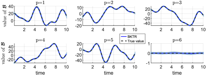
(a) Estimated coefficients at location $m=3$, i.e., $\boldsymbol{\mathcal{B}}(3,:,p=1,2,3,4,5,6)$ (mean with 95% CI in blue, true value in black).

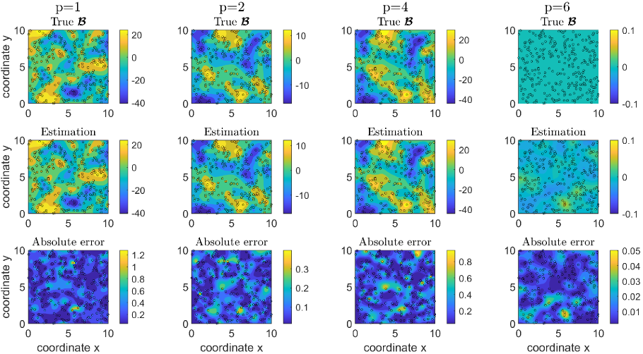
(b) Interpolated spatial surfaces of true value, estimated value (posterior mean), and absolute estimation error of the coefficients at time point $n=20$, i.e., $\boldsymbol{\mathcal{B}}(:,20,p=1,2,3,4,5,6)$. Black circles denote the positions of sampled locations.

Figure 3: BKTR ($R=10$) estimated coefficients for Simulation 1 (50% of $\boldsymbol{Y}$ is observed).

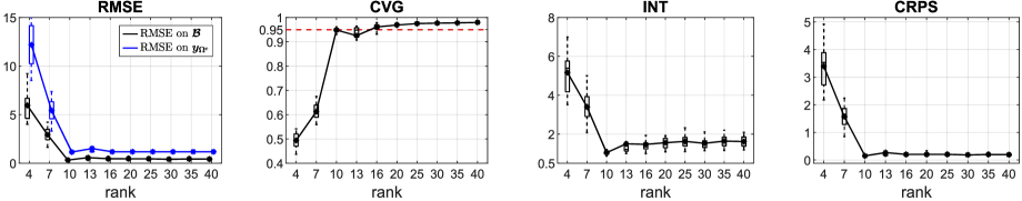
(a) Effect of the rank $R$.

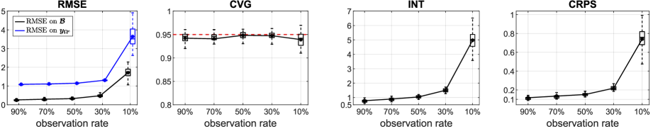
(b) Effect of the observation rate, i.e., $\frac{|\Omega|}{MN}$.

Figure 4: Sensitivity test of BKTR for Simulation 1. For each case, the figure shows the boxplot and mean value of corresponding metrics calculated from the 40 replications.

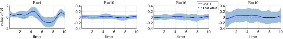
(a) Coefficients ($\boldsymbol{\mathcal{B}}(3,:,6)$) estimated by BKTR with different rank settings (when 50% of data is observed).

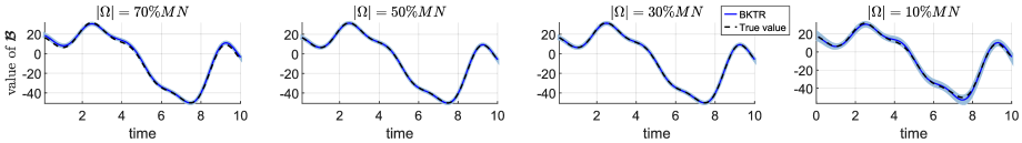
(b) Coefficients ($\boldsymbol{\mathcal{B}}(3,:,3)$) estimated by BKTR (with $R=10$) under different observation rates.

Figure 5: Comparison of BKTR in different settings for Simulation 1. (a) and (b) plot the estimated $\boldsymbol{\mathcal{B}}$ (mean with 95% CI) of one simulation at location #3 ($m=3$) for the 6th and 3rd covariates (i.e., $\boldsymbol{\mathcal{B}}(3,:,6)\text{ and }\boldsymbol{\mathcal{B}}(3,:,3)$), respectively.

The performances of BKTR with different rank specifications and 50% of the data points observed are compared in Figure 4 (a). We see that when the rank is over-specified (larger than the true value, i.e., $R>10$), BKTR can still achieve reliable estimation accuracy for both coefficients and unobserved data, even when $R$ is much larger than 10, e.g., $R=40$. The CVG for the 95% CI of $\boldsymbol{\mathcal{B}}$ is also maintained around 95% when $R>10$, the corresponding INT and CRPS keep a low value. This indicates that BKTR is able to provide accurate estimation for the coefficients along with high quality uncertainty even when the model includes redundant parameters. In addition, Figure 4 (b) illustrates the effect of the observation rate of $\boldsymbol{Y}$, where the results of BKTR (specifying $R=10$) with different proportions of observed data are compared. We observe that BKTR has a stable low estimation error when the rate of observed data decreases, and it continues to obtain valid CIs despite the increased lengths of CI for lower observation rates (i.e., the INT becomes larger). These results demonstrate the powerful applicability of the proposed Bayesian framework. We further show the temporal estimations of coefficients at a given location obtained in different cases in Figure 5. The plots in Panel (a) indicate that higher rank specification generates broader intervals, which is consistent with the results given in Figure 4 (a), i.e., the INT slightly increases with over-specified ranks. Panel (b) shows that BKTR can accurately estimate time-varying coefficients even when only 10% of the response data is observed, proving its high modeling capacity.

4.2 Simulation 2: model comparison on a small data set

4.2.1 Simulation setting

In this simulation, we generate a small data set in which the true $\boldsymbol{\mathcal{B}}$ is directly generated following a separable covariance matrix. Specifically, we simulate 30 locations $(M=30)$ in a $[0,10]\times[0,10]$ square and $N=30$ uniformly distributed time points in $[0,10]$. We then generate a small synthetic data set ${\left\{\boldsymbol{Y}\in\mathbb{R}^{30\times 30},\boldsymbol{\mathcal{X}}\in\mathbb{R}^{30\times 30\times 3}\right\}(P=3)}$ following Eq. (5) with:

$$\boldsymbol{\cal{X}}(:,:,1) =\operatorname{ones}(M,N),\ \boldsymbol{\cal{X}}(:,:,2)=\boldsymbol{1}_{N}^{\top}\otimes\boldsymbol{x}_{s},\ \boldsymbol{\cal{X}}(:,:,3)=\boldsymbol{1}_{M}\otimes\boldsymbol{x}_{t}^{\top},$$

$$\operatorname{vec}\left(\boldsymbol{B}_{(3)}\right) \sim\mathcal{N}\left(\boldsymbol{0},\boldsymbol{K}_{t}\otimes\boldsymbol{K}_{s}\otimes\boldsymbol{\Lambda}_{w}^{-1}\right),~{}\boldsymbol{\epsilon}\sim\mathcal{N}(\boldsymbol{0},\tau^{-1}\boldsymbol{I}_{MN}),$$

where ${\boldsymbol{x}_{s}\sim\mathcal{N}(\boldsymbol{0},\boldsymbol{I}_{M})}$, ${\boldsymbol{x}_{t}\sim\mathcal{N}(\boldsymbol{0},\boldsymbol{I}_{N})}$, ${\boldsymbol{K}_{s}}$ and ${\boldsymbol{K}_{t}}$ are still computed from a Matern 3/2 kernel and a SE kernel, respectively, and ${\boldsymbol{\Lambda}_{w}\sim\mathcal{W}(\boldsymbol{I}_{P},P)}$. For model parameters, we set the kernel variance hyperparameters to $\sigma_{s}^{2}=\sigma_{t}^{2}=2$, and consider combinations of data noise variance $\tau^{-1}\in\{0.2,1,5\}$, and kernel length-scale hyperparameters $\phi=\gamma\in\{1,2,4\}$. We specify the CP rank ${R=10}$ for BKTR estimation and compare BKTR with the original STVC model (Gelfand et al., 2003) and a pure low-rank Bayesian probabilistic tensor regression (BTR) model without imposing any spatiotemporal GP priors, using the same rank as BKTR. For both BKTR and STVC, we assume that the kernel functions are known, i.e., $k_{s}$ is Matern 3/2 and $k_{t}$ is SE, and use MCMC to estimate the unknown kernel hyperparameters. As in the previous simulations, we add a normally distributed non-significant random covariate in $\boldsymbol{\mathcal{X}}$ when fitting the model. We replicate each simulation 25 times and run the MCMC sampling with $K_{1}=1000$ and $K_{2}=500$.

4.2.2 Results

Table 2 presents the accuracy (mean$\pm$std) of the estimated coefficient tensor $\boldsymbol{\cal{B}}$ obtained from the 25 simulations. We also report the average computing time for each MCMC iteration. As we can see, BKTR with rank $R=10$ achieves similar accuracy as STVC and even performs better when increasing the data noise or kernel length-scales. This means that BKTR is more robust for noisy data and the low-rank assumption can fit the spatiotemporal relations better when they vary more smoothly/slowly. In addition, BKTR also clearly outperforms BTR, which confirms the importance of introducing GPs to encode the spatial and temporal dependencies. These results suggest that the proposed kernelized CP decomposition can approximate the true coefficient tensor relatively well even if the true $\boldsymbol{\cal{B}}$ does not follow an exact low-rank specification. In terms of computing time, we see that BKTR is much faster than STVC. Due to the high cost of STVC, it becomes infeasible to analyze a data set of moderate size, e.g., $M,N=100$, and $P=10$.

Table 2: Performance comparison for Simulation 2 $\left(\text{MAE}_{\boldsymbol{\mathcal{B}}}/\text{RMSE}_{\boldsymbol{\mathcal{B}}}\right)$.

Settings		STVC	BKTR	BTR
$\tau^{-1}=0.2$	$\phi=\gamma=1$	0.64$\pm$0.16/1.00$\pm$0.29	0.81$\pm$0.19/1.32$\pm$0.32	1.00$\pm$0.29/1.57$\pm$0.49
	$\phi=\gamma=2$	0.63$\pm$0.15/1.09$\pm$0.23	0.61$\pm$0.18/1.06$\pm$0.34	0.94$\pm$0.35/1.54$\pm$0.62
	$\phi=\gamma=4$	0.53$\pm$0.11/0.88$\pm$0.19	0.40$\pm$0.13/0.70$\pm$0.28	0.74$\pm$0.29/1.24$\pm$0.54
$\tau^{-1}=1$	$\phi=\gamma=1$	0.82$\pm$0.10/1.25$\pm$0.24	0.79$\pm$0.18/1.23$\pm$0.33	1.00$\pm$0.25/1.55$\pm$0.44
	$\phi=\gamma=2$	0.63$\pm$0.07/0.92$\pm$0.15	0.60$\pm$0.12/0.96$\pm$0.22	0.85$\pm$0.23/1.33$\pm$0.41
	$\phi=\gamma=4$	0.54$\pm$0.09/0.74$\pm$0.16	0.45$\pm$0.09/0.71$\pm$0.17	0.73$\pm$0.22/1.18$\pm$0.42
$\tau^{-1}=5$	$\phi=\gamma=1$	1.09$\pm$0.12/1.60$\pm$0.19	0.89$\pm$0.14/1.32$\pm$0.23	1.10$\pm$0.16/1.66$\pm$0.27
	$\phi=\gamma=2$	0.92$\pm$0.12/1.31$\pm$0.18	0.75$\pm$0.11/1.11$\pm$0.20	1.01$\pm$0.16/1.52$\pm$0.30
	$\phi=\gamma=4$	0.78$\pm$0.08/1.08$\pm$0.14	0.61$\pm$0.07/0.89$\pm$0.14	0.90$\pm$0.15/1.37$\pm$0.29
Average computing time		$\approx$15.44 sec/iter.	$\approx$0.011 sec/iter.	$\approx$0.008 sec/iter.

Figure 6 shows the estimation results of the three approaches for one chain/simulation when $\tau^{-1}=1,\phi=\gamma=1$. We plot an example for the third covariate at location #8 ($m=8,p=3$) to show the temporal variation of the coefficients estimated by the three methods. More comparison results in other settings are given in Appendix D.1. As can be seen, BKTR and STVC generate similar results and most of the coefficients are contained in the 95% CI for these two models. Although BTR can still capture the general trend, it fails to reproduce the local temporal dependency due to the absence of spatial/temporal priors. To further verify the mixing of the GP hyperparameters, we run the MCMC for BKTR for 5000 iterations and show the trace plots and probability distributions (after burn-in) for $\phi$ and $\gamma$ obtained when $\tau^{-1}=1,\phi=\gamma\in\{1,2,4\}$ in Figure 7. We can see that the Markov chains for the kernel hyperparameters mix fast and well, and a few hundred iterations should be sufficient for posterior inference.

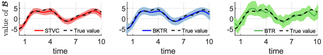
Figure 6: Comparison of the estimated coefficients when $\tau^{-1}=1,\phi=\gamma=1$. We show the approximated coefficients (mean with 95% CI) for the third covariate at location #8.

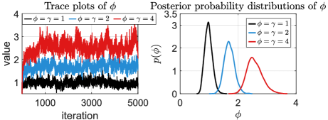
(a) Estimated hyperparameters of $\boldsymbol{K}_{s}$.

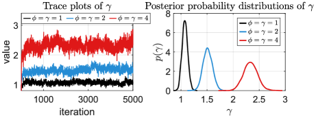
(b) Estimated hyperparameters of $\boldsymbol{K}_{t}$.

Figure 7: Kernel hyperparameters estimated by BKTR for Simulation 2 when $\tau^{-1}=1$.

4.3 Simulation 3: STVC modeling on a moderate-sized data set

4.3.1 Simulation setting

To evaluate the performance of BKTR in more realistic settings where the data size is large and the relationships are usually captured without low-rank structure, we further generate a relatively large synthetic data set of the same size as in Simulation 1, i.e., $M=300$ locations and $N=100$ time points. We generate the covariates $\boldsymbol{\mathcal{X}}\in\mathbb{R}^{300\times 100\times 5}~{}(P=5)$ according to Eq. (14). The coefficients are simulated using $\operatorname{vec}\left(\boldsymbol{B}_{(3)}\right)\sim\mathcal{N}\left(\boldsymbol{0},\boldsymbol{K}_{t}\otimes\boldsymbol{K}_{s}\otimes\boldsymbol{\Lambda}_{w}^{-1}\right)$. The parameters $\left\{\boldsymbol{K}_{s},\boldsymbol{K}_{t},\boldsymbol{\Lambda}_{w}\right\}$ and $\boldsymbol{\epsilon}$ are specified as in Simulation 1, i.e., $\boldsymbol{K}_{s}$ and $\boldsymbol{K}_{t}$ are computed from a Matern 3/2 and a SE kernel respectively with hyperparamaters $\{\sigma_{s}^{2}=\sigma_{t}^{2}=2,\phi=\gamma=1\}$, $\boldsymbol{\Lambda}_{w}\sim\mathcal{W}(\boldsymbol{I}_{P},P)$, and $\tau^{-1}=1$. We randomly select 50% of the generated data $\boldsymbol{Y}$ as observed responses. To assess the effect of the rank specification, we try different CP rank settings $R$ in $\{5,10,\cdots,60\}$ and compute MAE and RMSE for both $\boldsymbol{\mathcal{B}}$ and $\boldsymbol{y}_{\Omega^{c}}$. We replicate the experiment with each rank setting 15 times and run the MCMC sampling with $K_{1}=1000$ and $K_{2}=500$.

4.3.2 Results

Figure 8 shows the temporal behaviours of the estimated coefficients of four covariates in one simulation when $R=40$. The spatial patterns of the corresponding coefficients are provided in Appendix D.2. As one can see, BKTR can effectively reproduce the true values with acceptable errors. Figure 9 shows the effect of the rank. We see that choosing a larger rank $R$ gives better accuracy in terms of both $\text{MAE}_{\boldsymbol{\mathcal{B}}}/\text{RMSE}_{\boldsymbol{\mathcal{B}}}$ and $\text{MAE}_{\boldsymbol{y}_{\Omega^{c}}}/\text{RMSE}_{\boldsymbol{{y}}_{\Omega^{c}}}$. However, the accuracy gain becomes marginal when $R>30$. This demonstrates that the proposed Bayesian treatment offers a flexible solution in terms of model estimation and parameter inference.

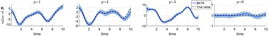
Figure 8: BKTR ($R=40$) estimated coefficients for Simulation 3. The figure plots the estimated $\boldsymbol{\mathcal{B}}$ (mean with 95% CI) of 4 covariates at location $m=3$, i.e., $\boldsymbol{\mathcal{B}}(3,:,p=1,4,5,6)$.

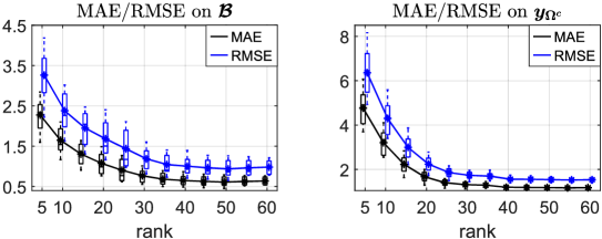
Figure 9: The effect of rank for Simulation 3. The figure shows the boxplot and mean of the estimation error on $\boldsymbol{\mathcal{B}}$ and $\boldsymbol{y}_{\Omega^{c}}$ with respect to the tensor rank.

5 Bike-sharing Demand modeling

5.1 Data description

In this section we perform local spatiotemporal regression on a large-scale bike-sharing trip data set collected from BIXI—a docked bike-sharing service in Montreal, Canada. BIXI operates 615 stations across the city and the yearly service time window is from April to November. We collect the number of daily departures for each station over $N=196$ days (from April 15 to October 27, 2019). We discard the stations with an average daily demand of less than 5, and only consider the remaining $M=587$ stations. The matrix $\boldsymbol{Y}$ contains $13.0\%$ unobserved/corrupted values in the raw data, and we only keep the rest as the observed set $\Omega$. We follow the analysis in (Faghih-Imani et al., 2014) and (Wang et al., 2021), and consider two types of spatial covariates: (a) features related to cycling infrastructure, and (b) land-use and built environment features. For temporal covariates, we mainly consider weather conditions and holidays. Table 3 lists the 13 spatial covariates $(\boldsymbol{x}_{s}^{p}\!\in\!\mathbb{R}^{M})$ and 5 temporal covariates $(\boldsymbol{x}_{t}^{p}\!\in\!\mathbb{R}^{N})$ used in this analysis. The final number of covariates is $P\!=\!13+5+1\!=\!19$, including the intercept. In constructing the covariate tensor $\boldsymbol{\mathcal{X}}$, we follow the same approach as in the simulation experiments. Specifically, we set $\boldsymbol{\cal{X}}(:,:,1)\!=\!\operatorname{ones}(M,N)$, and fill the rest of the tensor slices with $\boldsymbol{1}_{N}^{T}\otimes\boldsymbol{x}_{s}^{p}~{}(p=2:14)$ for the spatial covariates and $\boldsymbol{1}_{M}\otimes(\boldsymbol{x}_{t}^{p})^{\top}~{}(p=15:19)$ for the temporal covariates. Given the difference in magnitudes, we normalize all the covariates to $[0,1]$ using a min-max normalization. Since we use a zero-mean GP to parameterize $\boldsymbol{\beta}$, we normalize departure trips by removing the global effect of all covariates through a linear regression and consider $\boldsymbol{y}$ to be the unexplained part. The coefficient tensor $\boldsymbol{\cal{B}}$ contains more than $2\times 10^{6}$ entries, preventing us from using STVC directly.

Table 3: Description summary of independent variables.

spatial	(a)	length of cycle paths; length of major roads; length of minor roads; station capacity;
	(b)	numbers of metro stations, bus stations, and bus routes; numbers of restaurants, universities, other business & enterprises; park area; walkscore; population;
temporal		daily relative humidity; daily maximum temperature; daily mean temperature; total precipitation; dummy variables for holidays.

5.2 Experimental setup

For the spatial factors, we use a Matern 3/2 kernel as a universal prior, i.e., $k_{s}(\boldsymbol{s}_{m},\boldsymbol{s}_{m^{\prime}})=\left(1+\frac{\sqrt{3}d}{\phi}\right)\exp{\left(-\frac{\sqrt{3}d}{\phi}\right)}$, where $d$ is the haversine distance between locations $\boldsymbol{s}_{m}$ and $\boldsymbol{s}_{m^{\prime}}$, and $\phi$ is the spatial length-scale. The Matern class kernel is commonly used as a prior kernel function in spatial modeling. For the temporal factors, we use a locally periodic correlation matrix by taking the product of a periodic kernel and a SE kernel, i.e., $k_{t}(t_{n},t_{n^{\prime}})=\exp{\left(-\frac{2\sin^{2}{(\pi(t_{n}-t_{n^{\prime}})/T)}}{\gamma_{1}^{2}}-\frac{(t_{n}-t_{n^{\prime}})^{2}}{2\gamma_{2}^{2}}\right)}$, where $\gamma_{1}$ and $\gamma_{2}$ denote the length-scale and decay-time for the periodic component, respectively, and we fix the period as $T=7$ days. This specification suggests a weekly temporal pattern that can change over time, and it allows us to characterize both the daily variation and the weekly trend of the coefficients. We set the CP rank $R=20$, and run MCMC with $K_{1}=500$ and $K_{2}=500$ iterations.

5.3 Results

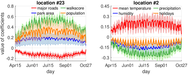
(a) Temporal plots of coefficients.

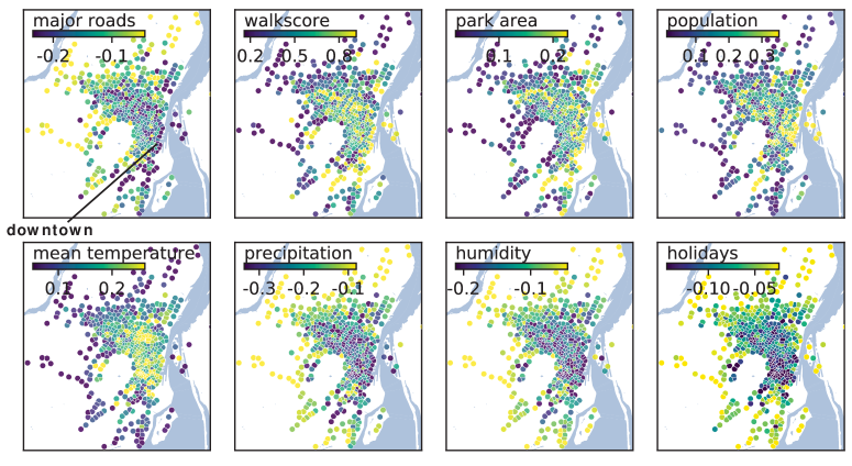
(b) Spatial maps of coefficients on August 1, 2019 $(n=109)$.

Figure 10: BKTR estimated coefficients for BIXI demand data. (a) Temporal plots of coefficients for 4 spatial covariates at location #23 $(m=23)$ and 4 temporal covariates at location #2 $(m=2)$, which show the mean with 95% CI. (b) Spatial maps showing the posterior mean for 8 covariates.

Figure 10 demonstrates some examples of the estimated coefficients, with panel (a) showing temporal examples of $\boldsymbol{\cal{B}}(\boldsymbol{s}_{m},:,:)$ and panel (b) showing spatial examples of $\boldsymbol{\cal{B}}(:,t_{n},:)$. As we can see in Figure 10(a), the temporal variation of the coefficients for both spatial and temporal covariates are interpretable. The coefficients (along with CI describing the uncertainty) allow us to identify the most important factors for each station at each time point. For example, we observe a similar variation over a week and a general long-term trend from April to October. Furthermore, the magnitude of the coefficients is much larger during the summer (July/August) compared to the beginning and end of the operation period, which is as expected as the outdoor temperature drops. Overall, for the spatial variables, the positive correlation of walkability and the negative impact caused by the length of major roads indicate that bicycle demands tend to be higher in densely populated neighborhoods. For the temporal covariates, precipitation, humidity and the holiday variable all relate to negative coefficients, implying that people are less likely to ride bicycles in rainy/humid periods and on holidays. The spatial distributions of the coefficients in Figure 10(b) also demonstrate consistent estimations, where the effects of covariates tend to be more obvious in the downtown area, involving coefficients with larger absolute values. Again, one can further explore the credible intervals to evaluate the significance of each covariate at a given location. It should be noted that the estimated variance $\tau^{-1}$ for $\boldsymbol{\epsilon}$ gives a posterior mean of $5.01\times 10^{-3}$ with a 95% CI of $[4.94,5.07]\times 10^{-3}$. This variance is much smaller compared with the variability of the data, confirming the importance of varying coefficients in the model. In summary, BKTR produces interpretable results for understanding the effects of different spatial and temporal covariates on bike-sharing demand. These findings can help planners to evaluate the performance of bike-sharing systems and update/design them.

5.4 Spatial interpolation

Due to the introduction of GP, BKTR is able to perform spatial prediction, i.e., kriging, for unknown locations, and such results can be used to select sites for new stations. To validate the spatial prediction/interpolation capacity, we randomly select 30% locations of the BIXI data set to be missing, and compute the prediction accuracy for these missing/testing data ($\boldsymbol{y}_{\Omega^{c}}$). Given that STVC is not applicable for a data set of such size, we compare BKTR (rank $R=20$) with SVC (spatially varying coefficient processes model) (Gelfand et al., 2003) which omits the modeling in time dimension. We also test BKTR and SVC in the case where both 30% locations and 30% time periods are missing. The prediction errors are given in Table 4, where we show the RMSE and MAPE (mean absolute percentage error) on $\boldsymbol{y}_{\Omega^{c}}$. MAPE is used to illustrate the relative error, and the definition is also provided in Appendix C. It is obvious that BKTR offers better performances with lower estimation errors in both missing scenarios, indicating its effectiveness in spatial prediction for real-world spatiotemporal data sets that often contain complicated missing/corruption patterns.

Table 4: Prediction performance for BIXI bike-sharing demand $\left(\text{RMSE}_{\boldsymbol{y}_{\Omega^{c}}}/\text{MAPE}_{\boldsymbol{y}_{\Omega^{c}}}\right)$.

Models	30% location missing	30% location with 30% time missing
SVC	0.26/5.84	0.20/4.22
BKTR ($R=20$)	0.22/4.45	0.17/3.24

6 Discussion

6.1 Identifiability and convergence of the model

In the regression problem studied in this paper, the kernel/covariance hyperparameters, $\text{i.e., }\{\phi,\gamma\}$, interpret/imply the correlation structure of the data, and the coefficients, i.e., $\boldsymbol{\mathcal{B}}$, reveal the spatiotemporal processes of the underlying associations. Thus, we consider the identifiability and convergence of kernel hyperparameters and the coefficients to be crucial. In contrast, note that the identifiability of latent factors decomposed from $\boldsymbol{\mathcal{B}}$ are not that important. For instance, our model is invariant in applying the same column permutation to the three factor matrices. From the results in simulation experiments (see Figure 7), it is clear that the Markov chains for kernel hyperparameters converge fast and well when using the proposed BKTR model. BKTR can also yield identifiable hyperparameters and reliable estimations for the coefficients.

6.2 The superiority of the BKTR framework

As we can see from the test of different rank settings and observation rates in the simulation experiments (see Figure 4 and 9), BKTR is able to provide high estimation accuracy and valid CIs even with a much larger or over-specified rank, and also effectively estimates the coefficients and the unobserved output values when only 10% of the data is observed. This indicates the advantage of the proposed Bayesian low-rank framework. Since we introduce a fully Bayesian sampling treatment for the kernelized low-rank tensor model which is free from parameter tuning, BKTR can estimate the model parameters and hyperparameters even when only a small number of observations are available. Thus, the model can avoid the over-fitting issue and consistently offer reliable estimation results, implying its effectiveness and usability for real-world complex spatiotemporal data analysis.

Another benefit of the proposed framework is the highly improved computing efficiency. Compared to the original STVC approach (Gelfand et al., 2003), which requires $\mathcal{O}\left(|\Omega|^{3}\right)$ for hyperparameter learning and $\mathcal{O}\left(|\Omega|^{3}P^{3}\right)$ for coefficient variable learning, BKTR reduces both of these computational costs to $\mathcal{O}\left(R^{3}\left(M^{3}+N^{3}+P^{3}\right)\right)$. The complexity can be further decreased to $\mathcal{O}\left(R\left(M^{3}+N^{3}+P^{3}\right)\right)$ by updating the correlation matrices for each column of factors separately and meanwhile sampling factors column by column. Such substantial gains in computing time allows us to analyze large-scale real-world spatiotemporal data and multi-dimensional relations, where generally the STVC is infeasible.

6.3 Counterpart kernel expression for $\boldsymbol{\beta}$

It has been shown that the classical low-rank tensor regression is equivalent to learning a multi-linear GP model with covariance matrix being the Kronecker product of several low-rank kernels capturing the correlations across different dimensions (Chu & Ghahramani, 2009; Yu et al., 2018). Furthermore, the general probabilistic CP decomposition for the coefficient tensor $\boldsymbol{\mathcal{B}}$ can be formulated as:

$$\boldsymbol{\mathcal{B}}=\sum_{r=1}^{R}s_{r}\times\left(\boldsymbol{u}_{r}\circ\boldsymbol{v}_{r}\circ\boldsymbol{w}_{r}\right),\ s_{r}\sim\mathcal{N}\left(0,1\right)\text{ for }r=1,\cdots,R,\ R\leq\min\{M,N\}.$$ (15)

By marginalizing over $\boldsymbol{\beta}$, we have the marginal distribution of the data

$$\boldsymbol{y}_{\Omega}\;|\;\boldsymbol{U},\boldsymbol{V},\boldsymbol{W}\sim\mathcal{N}\Big{(}\boldsymbol{0},\boldsymbol{O}\underbrace{\left(\sum_{r=1}^{R}\left(\boldsymbol{v}_{r}\boldsymbol{v}_{r}^{\top}\right)\otimes\left(\boldsymbol{u}_{r}\boldsymbol{u}_{r}^{\top}\right)\otimes\left(\boldsymbol{w}_{r}\boldsymbol{w}_{r}^{\top}\right)\right)}_{\boldsymbol{K}_{\beta}}\boldsymbol{O}^{\top}+\tau^{-1}\boldsymbol{I}_{|\Omega|}\Big{)}.$$ (16)

In this sense, the CP decomposition-based tensor regression is equivalent to learning $\boldsymbol{\beta}$ with a covariance matrix comprised of the sum of $R$ separable kernel matrices in which each component is a rank-one matrix. The key difference is that in BKTR we impose spatial/temporal GP priors on $\boldsymbol{u}_{r}\in\mathbb{R}^{M}\sim\mathcal{GP}(\boldsymbol{0},\boldsymbol{K}_{s})$ and $\boldsymbol{v}_{r}\in\mathbb{R}^{N}\sim\mathcal{GP}(\boldsymbol{0},\boldsymbol{K}_{t})$, and a Wishart prior on $\boldsymbol{w}_{r}\in\mathbb{R}^{P}\sim\mathcal{N}(\boldsymbol{0},\boldsymbol{\Lambda}^{-1})$.

We can also choose the probabilistic Tucker decomposition (Kolda & Bader, 2009) to parameterize $\boldsymbol{\beta}$ as a rank-$(R_{1},R_{2},R_{3})$ Tucker tensor with $R_{1}<M$, $R_{2}<N$ and $R_{3}<P$:

$$\boldsymbol{\mathcal{B}}=\sum_{r_{1}=1}^{R_{1}}\sum_{r_{2}=1}^{R_{2}}\sum_{r_{3}=1}^{R_{3}}s_{r_{1},r_{2},r_{3}}\times\left(\boldsymbol{u}_{r_{1}}\circ\boldsymbol{v}_{r_{2}}\circ\boldsymbol{w}_{r_{3}}\right),$$ (17)

where $\boldsymbol{\cal{S}}=\left(s_{r_{1},r_{2},r_{3}}\right)\in\mathbb{R}^{R_{1}\times R_{2}\times R_{3}}$ is the core tensor with $s_{r_{1},r_{2},r_{3}}\sim\mathcal{N}\left(0,1\right)$ for $r_{1}=1,\cdots,R_{1},\ r_{2}=1,\cdots,R_{2},\ r_{3}=1,\cdots,R_{3}$. We have the following marginal Gaussian distribution for observed data:

$$\boldsymbol{y}_{\Omega}\;|\;\boldsymbol{U},\boldsymbol{V},\boldsymbol{W}\sim\mathcal{N}\Big{(}\boldsymbol{0},\boldsymbol{O}\underbrace{\left(\boldsymbol{V}\boldsymbol{V}^{\top}\otimes\boldsymbol{U}\boldsymbol{U}^{\top}\otimes\boldsymbol{W}\boldsymbol{W}^{\top}\right)}_{\boldsymbol{K}_{\beta}}\boldsymbol{O}^{\top}+\tau^{-1}\boldsymbol{I}_{|\Omega|}\Big{)},$$ (18)

where $\boldsymbol{U}\in\mathbb{R}^{M\times R_{1}}$, $\boldsymbol{V}\in\mathbb{R}^{N\times R_{2}}$, and $\boldsymbol{W}\in\mathbb{R}^{P\times R_{3}}$. As we can see, this formulation imposes a similar separable kernel structure as in the original STVC model (Gelfand et al., 2003). When comparing Eq. (18) with $\boldsymbol{\beta}\sim\mathcal{N}(\boldsymbol{0},\boldsymbol{K}_{\beta_{t}}\otimes\boldsymbol{K}_{\beta_{s}}\otimes\boldsymbol{\Lambda}_{\beta}^{-1})$ in the original STVC, we see that the Tucker decomposition-based formulation translates to learning a low-rank approximation for each component correlation/covariance matrix in the separable kernel matrix (Yu et al., 2018). Note, however, that in Eq. (18) the spatial and temporal kernels are linear (e.g., $\boldsymbol{K}=\boldsymbol{U}\boldsymbol{U}^{\top}$) and thus they are nonstationary. To incorporate spatial and temporal dependencies, Tucker-based BKTR can also be designed by imposing spatial and temporal GP priors on the columns of $\boldsymbol{U}$ and $\boldsymbol{V}$. For example, if we assume each column of $\boldsymbol{U}$ follows an independent zero-mean GP, i.e., $\boldsymbol{u}_{r_{1}}\sim\mathcal{GP}\left(\boldsymbol{0},\boldsymbol{K}_{s}\right)$ for $r_{1}=1,\cdots,R_{1}$ with $\boldsymbol{K}_{s}$ being a spatial correlation matrix, we have the covariance matrix $\boldsymbol{K}=\boldsymbol{U}\boldsymbol{U}^{\top}\sim{\cal{W}}_{M}\left(\boldsymbol{K}_{s},R_{1}\right)$, which follows a singular Wishart distribution with degrees of freedom $R_{1}<M$ and scale matrix $\boldsymbol{K}_{s}$ (Uhlig, 1994). Thus, Tucker-BKTR becomes a computationally tractable approximation of STVC and its performance will largely depend on how well $\boldsymbol{K}_{\beta_{s}}$, $\boldsymbol{K}_{\beta_{t}}$ and $\boldsymbol{\Lambda}_{\beta}^{-1}$ can be approximated by the low-rank singular Wishart structure (up to a scaling constant). Overall, we can see that kernelized matrix/tensor decomposition provides a new approach to model multivariate spatial/spatiotemporal processes.

The low rank factorization-based models provide an alternative approach to model multivariate spatial/spatiotemporal processes, in particular when we have a large number of features (i.e., $P\gg 1$). It should be noted that estimating/marginalizing $\boldsymbol{U}$, $\boldsymbol{V}$ and $\boldsymbol{W}$ as latent factor matrices in Bayesian tensor regression/decomposition is much easier than estimating them as GP latent variables in the covariance function in Eqs. (16) and (18) (Lawrence, 2003; Li et al., 2009; Yu et al., 2018). Again, one can apply different kernel functions/hyperparameters as the prior for different columns of the factors, making the model more adaptive and flexible in characterizing the complex spatiotemporal patterns in the data. This will also lead to a more flexible Wishart distribution.

7 Conclusion

This paper introduces an effective solution for large-scale local spatiotemporal regression analysis. We propose parameterizing the model coefficients using low-rank CP decomposition, which greatly reduces the number of parameters from $M\times N\times P$ to $R(M+N+P)$. Contrary to previous studies on tensor regression, the proposed model BKTR goes beyond the low-rank assumption by integrating GP priors to characterize the strong local spatial and temporal dependencies. The framework also learns a low-rank multi-linear kernel which is expressive and able to provide insights for nonstationary and complicated processes. Our numerical experiments on both synthetic data and real-world data suggest that BKTR can reproduce the local spatiotemporal processes efficiently and reliably.

There are several directions for future research. In the current model, the CP rank $R$ needs to be specified in advance. One can make the model more flexible and adaptive by introducing a reasonably large core tensor with a multiplicative gamma process prior such as in Rai et al. (2014). The separable kernel assumption might be too restrictive, so the model can be further extended by introducing nonseparable kernel structure. In terms of GP priors, BKTR is flexible and can accommodate different kernels (w.r.t. function form and hyperparameter) for different factors such as in Luttinen & Ilin (2009). The combination of different kernels can also produce richer spatiotemporal dynamics and multiscale properties. In terms of computation, one can further reduce the cost in the GP learning (e.g., $\mathcal{O}(M^{3})$ for a spatial kernel) by further introducing sparse approximation techniques such as inducing points and predictive processes (Quinonero-Candela & Rasmussen, 2005; Banerjee et al., 2014). Lastly, the regression model itself can be extended from continuous to generalized responses, such as binary or count data, by introducing proper link functions (see e.g., Polson et al., 2013).

SUPPLEMENTARY MATERIAL

A Calculation of the marginal likelihood

We use the Woodbury matrix identity ${\footnotesize{(\boldsymbol{A}+\boldsymbol{C}\boldsymbol{B}\boldsymbol{C}^{\top})^{-1}=\boldsymbol{A}^{-1}-\boldsymbol{A}^{-1}\boldsymbol{C}\left(\boldsymbol{B}^{-1}+\boldsymbol{C}^{\top}\boldsymbol{A}^{-1}\boldsymbol{C}\right)^{-1}}}\\ {\footnotesize{\boldsymbol{C}^{\top}\boldsymbol{A}^{-1}}}$ to compute $\boldsymbol{K}_{\left.\boldsymbol{y}\right|\phi}^{-1}$, and further calculate $\boldsymbol{y}_{\Omega}^{\top}\boldsymbol{K}_{\left.\boldsymbol{y}\right|\phi}^{-1}\boldsymbol{y}_{\Omega}$ in Eq. (13) as follows:

$$\boldsymbol{y}_{\Omega}^{\top}\boldsymbol{K}_{\left.\boldsymbol{y}\right|\phi}^{-1}\boldsymbol{y}_{\Omega} =\boldsymbol{y}_{\Omega}^{\top}\left(\boldsymbol{H}_{U}\boldsymbol{K}_{U}\boldsymbol{H}_{U}^{\top}+\tau^{-1}\boldsymbol{I}_{|\Omega|}\right)^{-1}\boldsymbol{y}_{\Omega}$$

$$=\boldsymbol{y}_{\Omega}^{\top}\left(\tau\boldsymbol{I}_{|\Omega|}-\tau^{2}\boldsymbol{H}_{U}\left(\boldsymbol{K}_{U}^{-1}+\tau\boldsymbol{H}_{U}^{\top}\boldsymbol{H}_{U}\right)^{-1}\boldsymbol{H}_{U}^{\top}\right)\boldsymbol{y}_{\Omega}$$

$$=\tau\boldsymbol{y}_{\Omega}^{\top}\boldsymbol{y}_{\Omega}-\tau^{2}\boldsymbol{y}_{\Omega}^{\top}\boldsymbol{H}_{U}\left(\boldsymbol{I}_{R}\otimes\boldsymbol{K}_{s}^{-1}+\tau\boldsymbol{H}_{U}^{\top}\boldsymbol{H}_{U}\right)^{-1}\boldsymbol{H}_{U}^{\top}\boldsymbol{y}_{\Omega},$$

where $\boldsymbol{H}_{U}=\boldsymbol{O}\tilde{\boldsymbol{X}}_{U}\left((\boldsymbol{W}\odot\boldsymbol{V})\otimes\boldsymbol{I}_{M}\right)$ with $\tilde{\boldsymbol{X}}_{U}=\left(\boldsymbol{X}_{(3)}\odot\boldsymbol{I}_{MN}\right)^{\top}$. Based on the matrix determinant lemma $\left|\boldsymbol{A}+\boldsymbol{C}\boldsymbol{B}\boldsymbol{C}^{\top}\right|=\left|\boldsymbol{B}^{-1}+\boldsymbol{C}^{\top}\boldsymbol{A}^{-1}\boldsymbol{C}\right|\det{(\boldsymbol{B})}\det{(\boldsymbol{A})}$, the determinant in Eq. (13), i.e., $\log{\left|\boldsymbol{K}_{\left.\boldsymbol{y}\right|\phi}\right|}$, is computed as below:

$$\log{\left|\boldsymbol{K}_{\left.\boldsymbol{y}\right|\phi}\right|} =\log{\left|\boldsymbol{H}_{U}\boldsymbol{K}_{U}\boldsymbol{H}_{U}^{\top}+\tau^{-1}\boldsymbol{I}_{|\Omega|}\right|}$$

$$=\log{\left|\boldsymbol{I}_{R}\otimes\boldsymbol{K}_{s}^{-1}+\tau\boldsymbol{H}_{U}^{\top}\boldsymbol{H}_{U}\right|}+R\log{\left|\boldsymbol{K}_{s}\right|}-|\Omega|\log{\tau}.$$

Therefore, the log marginal posterior of $\phi$ is updated with:

$$\log{p\left(\phi\;\middle|\;\boldsymbol{y}_{\Omega},\boldsymbol{V},\boldsymbol{W},\tau,\boldsymbol{\mathcal{X}}\right)}\propto \log{p(\phi)}-\frac{1}{2}\boldsymbol{y}_{\Omega}^{\top}\boldsymbol{K}_{\left.\boldsymbol{y}\right|\phi}^{-1}\boldsymbol{y}_{\Omega}-\frac{1}{2}\log{\left|\boldsymbol{K}_{\left.\boldsymbol{y}\right|\phi}\right|}$$

$$\propto \log{p(\phi)}+\frac{1}{2}\tau^{2}\boldsymbol{y}_{\Omega}^{\top}\boldsymbol{H}_{U}\left(\boldsymbol{I}_{R}\otimes\boldsymbol{K}_{s}^{-1}+\tau\boldsymbol{H}_{U}^{\top}\boldsymbol{H}_{U}\right)^{-1}\boldsymbol{H}_{U}^{\top}\boldsymbol{y}_{\Omega}$$

$$-\frac{1}{2}\log{\left|\boldsymbol{I}_{R}\otimes\boldsymbol{K}_{s}^{-1}+\tau\boldsymbol{H}_{U}^{\top}\boldsymbol{H}_{U}\right|}-\frac{R}{2}\log{\left|\boldsymbol{K}_{s}\right|}.$$

B Sampling algorithm for kernel hyperparameters

The detailed sampling process for kernel hyperparmameters is provided in Algorithm 2.

Input: $\phi$, $\boldsymbol{V},\boldsymbol{W},\boldsymbol{y}_{\Omega},\boldsymbol{\mathcal{X}},\tau$.

Output: next $\phi$.

1 Initialize slice sampling scale $\rho=\log(10)$.

2 Compute $\boldsymbol{K}_{s},\boldsymbol{K}_{\left.\boldsymbol{y}\right|\phi},\log{p\left(\phi\;\middle|\;\boldsymbol{y}_{\Omega},\boldsymbol{V},\boldsymbol{W},\tau,\boldsymbol{\mathcal{X}}\right)}$ corresponding to $\phi$;

3 Calculate the sampling range: $\delta\sim\text{Uniform}(0,\rho)$, $\phi_{\min}=\phi-\delta$, $\phi_{\max}=\phi_{\min}+\rho$;

4 Draw $\eta\sim\text{Uniform}(0,1)$;

5 while True do

6       Draw proposal $\phi^{\prime}\sim\text{Uniform}(\phi_{\min},\phi_{\max})$;

7       Compute $\boldsymbol{K}_{s}^{\prime},\boldsymbol{K}_{\left.\boldsymbol{y}\right|\phi^{\prime}},\log{p\left(\phi^{\prime}\;\middle|\;\boldsymbol{y}_{\Omega},\boldsymbol{V},\boldsymbol{W},\tau,\boldsymbol{\mathcal{X}}\right)}$ corresponding to $\phi^{\prime}$;

8       if $\exp{\big{(}\log{p\left(\phi^{\prime}\;\middle|\;\boldsymbol{y}_{\Omega},\boldsymbol{V},\boldsymbol{W},\tau,\boldsymbol{\mathcal{X}}\right)}-\log{p\left(\phi\;\middle|\;\boldsymbol{y}_{\Omega},\boldsymbol{V},\boldsymbol{W},\tau,\boldsymbol{\mathcal{X}}\right)}\big{)}}>\eta$ then

9            return $\phi^{\prime}$; break;

10       else if $\phi^{\prime}<\phi$ then

11            $\phi_{\min}=\phi^{\prime}$;

12       else

13            $\phi_{\max}=\phi^{\prime}$.

14      

Algorithm 2 Sampling process for kernel hyperparameter $\phi$

C Evaluation metrics

The metrics for assessing the estimation accuracy on coefficients $\boldsymbol{\mathcal{B}}$ ($\text{MAE}_{\boldsymbol{\mathcal{B}}}/\text{RMSE}_{\boldsymbol{\mathcal{B}}}$) and unobserved output/response entries $\boldsymbol{y}_{\Omega^{c}}$ ($\text{MAE}_{\boldsymbol{y}_{\Omega^{c}}}/\text{RMSE}_{\boldsymbol{y}_{\Omega^{c}}}/\text{MAPE}_{\boldsymbol{y}_{\Omega^{c}}}$) are defined as:

$$\text{MAE}_{\boldsymbol{\mathcal{B}}}=\frac{1}{MNP}\sum_{m=1}^{M}\sum_{n=1}^{N}\sum_{p=1}^{P}\left|b_{mnp}-\hat{b}_{mnp}\right|,\text{RMSE}_{\boldsymbol{\mathcal{B}}}=\sqrt{\frac{1}{MNP}\sum_{m=1}^{M}\sum_{n=1}^{N}\sum_{p=1}^{P}\left(b_{mnp}-\hat{b}_{mnp}\right)^{2}},$$

$$\text{MAE}_{\boldsymbol{y}_{\Omega^{c}}}=\frac{1}{MNP-|\Omega|}\sum_{i\notin\Omega}\left|y_{i}-\hat{y}_{i}\right|,\text{RMSE}_{\boldsymbol{y}_{\Omega^{c}}}=\sqrt{\frac{1}{MNP-|\Omega|}\sum_{i\notin\Omega}\left(y_{i}-\hat{y}_{i}\right)^{2}},$$

$$\text{MAPE}_{\boldsymbol{y}_{\Omega^{c}}}=\frac{1}{MNP-|\Omega|}\sum_{i\notin\Omega}\left|\frac{y_{i}-\hat{y}_{i}}{y_{i}}\right|,$$

where $\hat{b}_{mnp}$ and $b_{mnp}$ are the $(m,n,p)$th element of the estimated and the setting/true coefficient tensor, respectively, $y_{i}$ and $\hat{y}_{i}$ are the actual value and estimation of $i$th unobserved data, respectively. The criteria related to quantifying the uncertainty performance, i.e., CVG (interval coverage), INT (interval score), and CRPS (continuous rank probability score) of the 95% posterior CI for the estimated $\boldsymbol{\mathcal{B}}$ values, are defined as follows:

$$\text{CVG}= \frac{1}{MNP}\sum_{m=1}^{M}\sum_{n=1}^{N}\sum_{p=1}^{P}\mathbbm{1}\left\{{b}_{mnp}\in\left[l_{mnp},u_{mnp}\right]\right\},$$

$$\text{INT}= \frac{1}{MNP}\sum_{m=1}^{M}\sum_{n=1}^{N}\sum_{p=1}^{P}\left(u_{mnp}-l_{mnp}\right)+\frac{2}{\alpha}\left(l_{mnp}-b_{mnp}\right)\mathbbm{1}\{b_{mnp}<l_{mnp}\}$$

$$~{}~{}~{}~{}~{}~{}~{}~{}~{}~{}~{}~{}~{}~{}~{}~{}~{}~{}~{}~{}~{}~{}~{}~{}~{}~{}~{}~{}~{}~{}~{}~{}~{}~{}~{}~{}~{}~{}~{}~{}~{}~{}~{}+\frac{2}{\alpha}\left(b_{mnp}-u_{mnp}\right)\mathbbm{1}\{b_{mnp}>u_{mnp}\},$$

$$\text{CRPS}= -\frac{1}{MNP}\sum_{m=1}^{M}\sum_{n=1}^{N}\sum_{p=1}^{P}\sigma_{mnp}\Bigg{[}\frac{1}{\sqrt{\pi}}-2\psi\left(\frac{b_{mnp}-\hat{b}_{mnp}}{\sigma_{mnp}}\right)$$

$$~{}~{}~{}~{}~{}~{}~{}~{}~{}~{}~{}~{}~{}~{}~{}~{}~{}~{}~{}~{}~{}~{}~{}~{}~{}~{}~{}~{}~{}~{}~{}~{}~{}~{}~{}~{}~{}-\frac{b_{mnp}-\hat{b}_{mnp}}{\sigma_{mnp}}\left(2\Phi\left(\frac{b_{mnp}-\hat{b}_{mnp}}{\sigma_{mnp}}\right)-1\right)\Bigg{]},$$

where $\psi$ and $\Phi$ denote the pdf (probability density function) and cdf (cumulative distribution function) of a standard normal distribution, respectively; $\sigma_{mnp}$ is the standard deviation (std.) of the estimation values after burn-in for $(m,n,p)$th entry of $\boldsymbol{\mathcal{B}}$, i.e., the std. of $\left\{\tilde{\boldsymbol{\mathcal{B}}}^{(k)}\right\}_{k=K_{1}+1}^{K_{1}+K_{2}}$, $\alpha=0.05$, $[l_{mnp},u_{mnp}]$ denotes the 95% central estimation interval for each coefficient value, and $\mathbbm{1}\{\cdot\}$ represents an indicator function that equals 1 if the condition is true and 0 otherwise.

D Supplementary results for simulation experiments

D.1 Simulation 2

For Simulation 2, Figure 11 shows the estimation results of STVC, BKTR, and BTR for one chain when $\tau^{-1}=1,\phi=\gamma\in\{2,4\}$. We still give the example for the third covariate at location #8 ($m=8,p=3$) to compare the estimated temporal variation of the coefficients by the three methods.

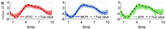
(a) $\tau^{-1}=1,\ \phi=\gamma=2$.

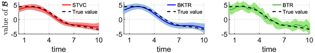
(b) $\tau^{-1}=1,\ \phi=\gamma=4$.

Figure 11: Comparison of the estimated coefficients for Simulation 2, where $\tau^{-1}=1,\phi=\gamma\in\{2,4\}$. We show the approximated coefficients (mean with 95% CI) for the third covariate at location #8.

D.2 Simulation 3

For Simulation 3, Figure 12 gives the spatial patterns of the BKTR estimated coefficients of four covariates in one simulation when $R=40$.

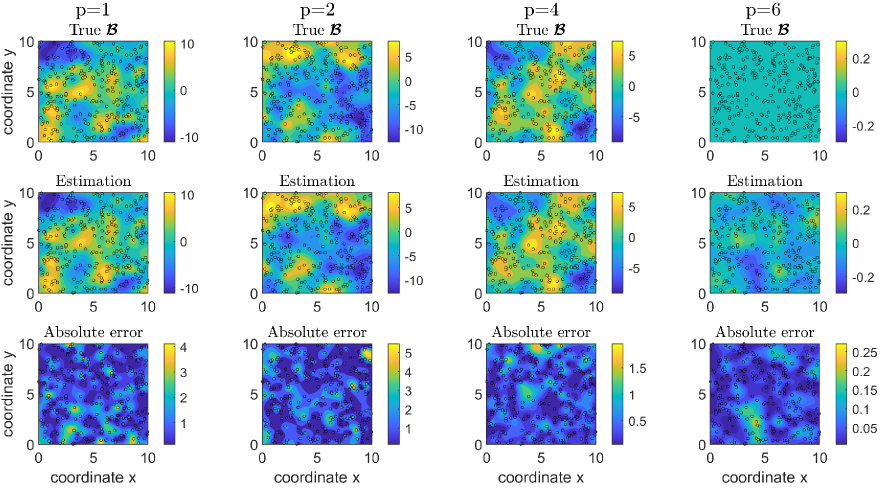
Figure 12: BKTR ($R=40$) estimated coefficients for Simulation 3. The figure shows the interpolated spatial surfaces of the estimated coefficients at time point $n=20$, i.e. $\boldsymbol{\mathcal{B}}(:,20,p=1,2,4,6)$, where black circles denote the positions of sampled locations.

References

- (1)
- Bahadori et al. (2014) Bahadori, M. T., Yu, Q. R. & Liu, Y. (2014), ‘Fast multivariate spatio-temporal analysis via low rank tensor learning’, Advances in Neural Information Processing Systems pp. 3491–3499.
- Banerjee et al. (2014) Banerjee, S., Carlin, B. P. & Gelfand, A. E. (2014), Hierarchical modeling and analysis for spatial data, CRC press.
- Chu & Ghahramani (2009) Chu, W. & Ghahramani, Z. (2009), ‘Probabilistic models for incomplete multi-dimensional arrays’, Artificial Intelligence and Statistics pp. 89–96.
- Cressie & Wikle (2015) Cressie, N. & Wikle, C. K. (2015), Statistics for spatio-temporal data, John Wiley & Sons.
- Faghih-Imani et al. (2014) Faghih-Imani, A., Eluru, N., El-Geneidy, A. M., Rabbat, M. & Haq, U. (2014), ‘How land-use and urban form impact bicycle flows: evidence from the bicycle-sharing system (bixi) in montreal’, Journal of Transport Geography 41, 306–314.
- Finley (2011) Finley, A. O. (2011), ‘Comparing spatially-varying coefficients models for analysis of ecological data with non-stationary and anisotropic residual dependence’, Methods in Ecology and Evolution 2(2), 143–154.
- Finley & Banerjee (2020) Finley, A. O. & Banerjee, S. (2020), ‘Bayesian spatially varying coefficient models in the spbayes r package’, Environmental Modelling & Software 125, 104608.
- Fotheringham et al. (2003) Fotheringham, A. S., Brunsdon, C. & Charlton, M. (2003), Geographically weighted regression: the analysis of spatially varying relationships, John Wiley & Sons.
- Gelfand et al. (2003) Gelfand, A. E., Kim, H.-J., Sirmans, C. & Banerjee, S. (2003), ‘Spatial modeling with spatially varying coefficient processes’, Journal of the American Statistical Association 98(462), 387–396.
- Gneiting & Raftery (2007) Gneiting, T. & Raftery, A. E. (2007), ‘Strictly proper scoring rules, prediction, and estimation’, Journal of the American statistical Association 102(477), 359–378.
- Guhaniyogi et al. (2017) Guhaniyogi, R., Qamar, S. & Dunson, D. B. (2017), ‘Bayesian tensor regression’, The Journal of Machine Learning Research 18(1), 2733–2763.
- Heaton et al. (2019) Heaton, M. J., Datta, A., Finley, A. O., Furrer, R., Guinness, J., Guhaniyogi, R., Gerber, F., Gramacy, R. B., Hammerling, D., Katzfuss, M. et al. (2019), ‘A case study competition among methods for analyzing large spatial data’, Journal of Agricultural, Biological and Environmental Statistics 24(3), 398–425.
- Huang et al. (2010) Huang, B., Wu, B. & Barry, M. (2010), ‘Geographically and temporally weighted regression for modeling spatio-temporal variation in house prices’, International Journal of Geographical Information Science 24(3), 383–401.
- Izenman (1975) Izenman, A. J. (1975), ‘Reduced-rank regression for the multivariate linear model’, Journal of Multivariate Analysis 5(2), 248–264.
- Kolda & Bader (2009) Kolda, T. G. & Bader, B. W. (2009), ‘Tensor decompositions and applications’, SIAM Review 51(3), 455–500.
- Lawrence (2003) Lawrence, N. (2003), ‘Gaussian process latent variable models for visualisation of high dimensional data’, Proceedings of the 16th International Conference on Neural Information Processing Systems pp. 329–336.
- Lei et al. (2022) Lei, M., Labbe, A., Wu, Y. & Sun, L. (2022), ‘Bayesian kernelized matrix factorization for spatiotemporal traffic data imputation and kriging’, IEEE Transactions on Intelligent Transportation Systems .
- Li et al. (2009) Li, W.-J., Zhang, Z. & Yeung, D.-Y. (2009), ‘Latent wishart processes for relational kernel learning’, Artificial Intelligence and Statistics pp. 336–343.
- Luttinen & Ilin (2009) Luttinen, J. & Ilin, A. (2009), ‘Variational gaussian-process factor analysis for modeling spatio-temporal data’, Advances in Neural Information Processing Systems 22, 1177–1185.
- Murray & Adams (2010) Murray, I. & Adams, R. P. (2010), ‘Slice sampling covariance hyperparameters of latent gaussian models’, Advances in Neural Information Processing Systems pp. 1723–1731.
- Neal (2003) Neal, R. M. (2003), ‘Slice sampling’, The annals of statistics 31(3), 705–767.
- Polson et al. (2013) Polson, N. G., Scott, J. G. & Windle, J. (2013), ‘Bayesian inference for logistic models using pólya–gamma latent variables’, Journal of the American statistical Association 108(504), 1339–1349.
- Quinonero-Candela & Rasmussen (2005) Quinonero-Candela, J. & Rasmussen, C. E. (2005), ‘A unifying view of sparse approximate gaussian process regression’, The Journal of Machine Learning Research 6, 1939–1959.
- Rabusseau & Kadri (2016) Rabusseau, G. & Kadri, H. (2016), ‘Low-rank regression with tensor responses’, Advances in Neural Information Processing Systems 29, 1867–1875.
- Rai et al. (2014) Rai, P., Wang, Y., Guo, S., Chen, G., Dunson, D. & Carin, L. (2014), ‘Scalable bayesian low-rank decomposition of incomplete multiway tensors’, International Conference on Machine Learning pp. 1800–1808.
- Rao et al. (2015) Rao, N., Yu, H.-F., Ravikumar, P. & Dhillon, I. S. (2015), ‘Collaborative filtering with graph information: Consistency and scalable methods’, Advances in Neural Information Processing Systems pp. 2107–2115.
- Rasmussen & Williams (2006) Rasmussen, C. E. & Williams, C. K. (2006), Gaussian Processes for Machine Learning, MIT Press.
- Saatçi (2012) Saatçi, Y. (2012), Scalable inference for structured Gaussian process models, PhD thesis, University of Cambridge.
- Uhlig (1994) Uhlig, H. (1994), ‘On singular wishart and singular multivariate beta distributions’, The Annals of Statistics pp. 395–405.
- Wang et al. (2021) Wang, X., Cheng, Z., Trépanier, M. & Sun, L. (2021), ‘Modeling bike-sharing demand using a regression model with spatially varying coefficients’, Journal of Transport Geography 93, 103059.
- Wilson et al. (2014) Wilson, A. G., Gilboa, E., Cunningham, J. P. & Nehorai, A. (2014), ‘Fast kernel learning for multidimensional pattern extrapolation’, Advances in Neural Information Processing Systems pp. 3626–3634.
- Yu et al. (2018) Yu, R., Li, G. & Liu, Y. (2018), ‘Tensor regression meets gaussian processes’, International Conference on Artificial Intelligence and Statistics pp. 482–490.
- Yu & Liu (2016) Yu, R. & Liu, Y. (2016), ‘Learning from multiway data: Simple and efficient tensor regression’, International Conference on Machine Learning pp. 373–381.
- Zhou et al. (2013) Zhou, H., Li, L. & Zhu, H. (2013), ‘Tensor regression with applications in neuroimaging data analysis’, Journal of the American Statistical Association 108(502), 540–552.