Half-Space and Box Constraints as NUV Priors: First Results

Abstract

Normals with unknown variance (NUV) can represent many useful priors and blend well with Gaussian models and message passing algorithms. NUV representations of sparsifying priors have long been known, and NUV representations of binary (and $M$-level) priors have been proposed very recently. In this document, we propose NUV representations of half-space constraints and box constraints, which allows to add such constraints to any linear Gaussian model with any of the previously known NUV priors without affecting the computational tractability.

I Introduction

NUV priors (normals with unknown variance) hugely extend the expressive power of linear Gaussian models while essentially maintaining their computational tractability by standard algorithms. NUV priors originated in sparse Bayesian learning [1, 2, 3, 4, 5, 6] and are closely related to variational representations of sparsifying priors [7, 8]. However, NUV priors can also represent smoothed versions of such priors (including the Huber function) [8], and it has very recently been shown that NUV priors can also represent discretizing priors [9, 10].

In this document, we show that NUV priors can also express half-space constraints (inequality constraints) and box constraints (interval constraints). This is not difficult (with hindsight), but it is very useful, as it allows to include such constraints in linear Gaussian models (with or without additional NUV priors), while maintaining their tractability by standard algorithms such as iterated least-squares [11, 12] or iterated versions of Kalman-type algorithms for linear Gaussian models, cf. [6, 8].

In formal terms, a half-space constraint on a quantity $x\in\mathbb{R}$ enforces the inequality

$$x\leq a\quad\text{or}\quad x\geq a,$$ (1)

with $a\in\mathbb{R}$. Similarly, a box constraint on $x$ enforces the inequality

$$a\leq x\leq b,$$ (2)

with $a,b\in\mathbb{R}$.

In the following, we will derive NUV prior representations of the constraints (1) and (2), where we assume that $x$ is a variable in some linear Gaussian model.

II NUV Representation of the Laplace Prior

To begin with, we provide a quick primer on the (well-known [7, 8]) NUV representation of the Laplace prior, as this will be a fundamental step for the derivation of the proposed prior models. The Laplace prior can be represented using a NUV prior of the form 

$$p(x)\triangleq\max_{\sigma^{2}}\mathcal{N}\!\left({x;a,\sigma^{2}}\right)\rho(\sigma),$$ (3)

where $\sigma^{2}$ is an unknown variance, $a\in\mathbb{R}$, and

$$\rho(\sigma)\triangleq\sqrt{2\pi\sigma^{2}}\exp\left({-\gamma^{2}\sigma^{2}/2}\right),$$ (4)

with $\gamma>0$. Note that for fixed $\sigma^{2}$, (3) is Gaussian, up to a scale factor.

Such variational representations of non-Gaussian priors in combination with an otherwise Gaussian model blend well with iterative algorithms that alternate between estimating $x$ (for fixed $\sigma^{2}$), for instance by least-squares or Kalman-type algorithms, and estimating $\sigma^{2}$ (for fixed $x$) by finding the maximizing $\sigma^{2}$ of (3). More specifically, for a given $x$, the maximizing $\sigma^{2}$ of (3) is easily determined to be

$$\hat{\sigma}^{2} = \operatorname*{argmax}_{\sigma^{2}}\mathcal{N}\!\left({x;a,\sigma^{2}}\right)\rho(\sigma),$$ (5)

$$= \operatorname*{argmin}_{\sigma^{2}}\frac{(x-a)^{2}}{\sigma^{2}}+\gamma^{2}\sigma^{2}$$ (6)

$$= |x-a|/\gamma.$$ (7)

Consequently, (3) amounts to

$$p(x)=\exp\left({-\gamma|x-a|}\right),$$ (8)

which is proportional to a Laplace prior, up to a scale factor.

Figure 1: The function $\kappa(x)=\gamma|x-a|$, for $\gamma=1$ and $a=0$.

The associated cost function is defined as

$$\kappa(x) \triangleq -\log p(x).$$ (9)

$$= \gamma|x-a|,$$ (10)

and is illustrated in Fig. 1. Throughout the remainder of this document, we will make frequent use of both the probabilistic view (as in (8)), and the perspective of a cost function (as (10)).

III Box Constraint

The NUV representation of the box constraint is an almost obvious combination of two well-known ideas: Namely, (i) the NUV representation of the Laplace prior of Section II, and (ii) adding two cost functions of the form (10) to a cost function that is constant for $x\in[a,b]$, as illustrated in Fig. 2. In formal terms, we consider a composite prior model of the form

$$p(x) \triangleq \max_{\theta}\mathcal{N}\!\left({x;a,\sigma_{a}^{2}}\right)\mathcal{N}\!\left({x;b,\sigma_{b}^{2}}\right)\rho(\sigma_{a})\rho(\sigma_{b})\psi(\gamma,a,b),$$

where $\theta=(\sigma_{a}^{2},\sigma_{b}^{2})$, and where

$$\rho(\sigma_{i})\triangleq\sqrt{2\pi\sigma_{i}^{2}}\exp(-\gamma^{2}\sigma_{i}^{2}/2),$$ (12)

for $i\in\{a,b\}$. The term $\psi(\gamma,a,b)$ is defined as

$$\psi(\gamma,a,b)\triangleq\exp(\gamma|b-a|),$$ (13)

for reasons which will be obvious later on. Note that (III) is Gaussian in $x$, up to a scale factor, and can equivalently be written as

$$p(x) = \max_{\theta}p(x\hskip 0.20004pt|\hskip 0.80002pt\theta)g(\theta),$$ (14)

where

$$p(x\hskip 0.20004pt|\hskip 0.80002pt\theta)=\mathcal{N}\!\left({x;m_{\theta},\sigma_{\theta}^{2}}\right),$$ (15)

with

$$m_{\theta} = \frac{a\sigma_{b}^{2}+b\sigma_{a}^{2}}{\sigma_{a}^{2}+\sigma_{b}^{2}},$$ (16)

$$\sigma_{\theta}^{2} = (1/\sigma_{a}^{2}+1/\sigma_{b}^{2})^{-1}=\frac{\sigma_{a}^{2}\sigma_{b}^{2}}{\sigma_{a}^{2}+\sigma_{b}^{2}},$$ (17)

and

$$g(\theta)=\mathcal{N}\!\left({0,a-b,\sigma_{a}^{2}+\sigma_{b}^{2}}\right)\rho(\sigma_{a})\rho(\sigma_{b})\psi(\gamma,a,b).$$ (18)

Note that $g(\theta)$ is independent of $x$.

Figure 2: Function $\kappa(x)=\gamma(|x\!-\!a|+|x\!-\!b|-|b\!-\!a|)$, for $a=-1,b=1$ and $\gamma=1$.

For a given $x$, the maximizing $\theta$ of (III) is easily determined to be

$$\hat{\theta}=(\hat{\sigma}_{a}^{2},\hat{\sigma}_{b}^{2})=\big{(}|x-a|/\gamma,|x-b|/\gamma\big{)}.$$ (19)

Plugging in (19) into (III) leads to

$$p(x)=\exp\left({-\gamma(|x-a|+|x-b|-|b-a|)}\right),$$ (20)

and consequently, the associated cost function amounts to

$$\kappa(x) \triangleq -\log p(x)=\gamma(|x-a|+|x-b|-|b-a|),$$ (21)

which is illustrated in Fig. 2. The free parameter $\gamma$ is used to obtain arbitrarily steep side lobes of $\kappa(x)$, for $x\notin[a,b]$. The term (13) shifts (21), such that $k(x)=0$, for $x\in[a,b]$.

We now examine the effect of this proposed prior model by assuming that $p(x)$ is used in some simple model with fixed observation(s) $\breve{y}$ and likelihood $p(\breve{y}\hskip 0.20004pt|\hskip 0.80002ptx)$, given by

$$p(\breve{y}\hskip 0.20004pt|\hskip 0.80002ptx)=\mathcal{N}\!\left({x;\mu,s^{2}}\right),$$ (22)

where $\mu$ and $s^{2}>0$ depend on $\breve{y}$. We assume that $x$ and $\theta$ are determined by joint Maximum-a-Posteriori (MAP) estimation according to

$$\hat{x} = \operatorname*{argmax}_{x}\max_{\theta}p(\breve{y}\hskip 0.20004pt|\hskip 0.80002ptx)p(x\hskip 0.20004pt|\hskip 0.80002pt\theta)g(\theta).$$ (23)

The statistical model (23) is illustrated as factor graph [13] in Fig. 3.

Figure 3: Factor graph of the statistical model (23).

The structure of (23) suggests algorithms that iterate between a maximization step over $x$ for fixed $\theta=\hat{\theta}$, and a maximization step over $\theta$ for fixed $x=\hat{x}$. The first step is entirely Gaussian, since for fixed $\theta$, (23) is Gaussian, up to a scale factor. In the second step, we compute

$$\hat{\theta}=\operatorname*{argmax}_{\theta}p(\breve{y}\hskip 0.20004pt|\hskip 0.80002ptx)p(x\hskip 0.20004pt|\hskip 0.80002pt\theta)g(\theta)=\operatorname*{argmax}_{\theta}p(x\hskip 0.20004pt|\hskip 0.80002pt\theta)g(\theta),$$ (24)

which coincides with (19).

Note that any such coordinate descent algorithm is guaranteed to converge to a local maximum or a saddle point, if the underlying objective function is smooth. Numerical results of (23) are plotted in Fig. 4, for $a=-1$, $b=1$, $\gamma=1$, and different values for $s^{2}$.

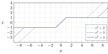
Figure 4: Estimate (23) for $a=-1$, $b=1$, $\gamma=1$, and different $s^{2}$.

We observe (and it can be proven) that for a given $\mu$ and $s^{2}$, and a sufficiently large $\gamma$, the estimate $\hat{x}$ lies in $[a,b]$. More specifically, the constraint (2) is satisfied, if and only if

$$s^{2}\geq\begin{cases}0,&\text{if $\mu\in[a,b]$}\\ \min\left\{\frac{|a-\mu|}{2\gamma},\frac{|b-\mu|}{2\gamma}\right\},&\mathrm{else}.\end{cases}$$ (25)

Note that since $\gamma$ is a free design parameter, (25) can essentially always be satisfied.

IV Half-Space Constraint

A half-space constraint can be obtained by using a box constraint as in Section III and letting one of the boundary points go to $\pm\infty$. We first consider the case for ${b\rightarrow\infty}$.

For ${b\rightarrow\infty}$, (19) is obviously not well-defined. However, if we consider (14) with (19) plugged in for ${b\rightarrow\infty}$, (14) remains well-defined. Specifically, we consider a prior of the form

$$p(x) \triangleq \lim_{b\rightarrow\infty}\max_{\theta}p(x\hskip 0.20004pt|\hskip 0.80002pt\theta)g(\theta)$$ (26)

$$= \lim_{b\rightarrow\infty}p(x\hskip 0.20004pt|\hskip 0.80002pt\hat{\theta})g(\hat{\theta}),$$ (27)

where $p(x\hskip 0.20004pt|\hskip 0.80002pt\theta)$ is as in (15), $g(\theta)$ is as in (18), and $\hat{\theta}$ as in (19). To show that (26) is well-defined, we first inspect the first two moments of $p(x\hskip 0.20004pt|\hskip 0.80002pt\hat{\theta})$ in the limit of ${b\rightarrow\infty}$, i.e.,

$$\tilde{m}_{\theta} \triangleq \lim_{b\rightarrow\infty}m_{\theta}\Big{\rvert}_{\theta=\hat{\theta}}$$ (28)

$$= \lim_{b\rightarrow\infty}\frac{a\hat{\sigma}_{b}^{2}+b\hat{\sigma}_{a}^{2}}{\hat{\sigma}_{a}^{2}+\hat{\sigma}_{b}^{2}}$$ (29)

$$= \lim_{b\rightarrow\infty}\frac{a|x-b|+b|x-a|}{|x-b|+|x-a|}$$ (30)

$$= \lim_{b\rightarrow\infty}\frac{b(|x-a|+a)-ax}{b-x+|x-a|}$$ (31)

$$\stackrel{{\scriptstyle\text{d'H\^{o}pital}}}{{=}} |x-a|+a$$ (32)

and

$$\tilde{\sigma}_{\theta}^{2} = \lim_{b\rightarrow\infty}\sigma_{\theta}^{2}\Big{\rvert}_{\theta=\hat{\theta}}$$ (33)

$$= \lim_{b\rightarrow\infty}\frac{\hat{\sigma}_{a}^{2}\hat{\sigma}_{b}^{2}}{\hat{\sigma}_{a}^{2}+\hat{\sigma}_{b}^{2}}$$ (34)

$$= \lim_{b\rightarrow\infty}\frac{|x-a|\cdot|x-b|}{\gamma(|x-a|+|x-b|)}$$ (35)

$$= \lim_{b\rightarrow\infty}\frac{|x-a|\cdot(b-x)}{\gamma(|x-a|+(b-x))}$$ (36)

$$\stackrel{{\scriptstyle\text{d'H\^{o}pital}}}{{=}} |x-a|/\gamma.$$ (37)

As a consequence,

$$\lim_{b\rightarrow\infty}p(x\hskip 0.20004pt|\hskip 0.80002pt\hat{\theta})=\mathcal{N}\!\left({x;\tilde{m}_{\theta},\tilde{\sigma}_{\theta}^{2}}\right)$$ (38)

which thus also well-defined. It remains to prove that $g(\hat{\theta})$ in (27) for ${b\rightarrow\infty}$ is also well-defined. For the sake of simplicity, we first consider

$$\lim_{b\rightarrow\infty} -\log g(\hat{\theta})$$

$$= \lim_{b\rightarrow\infty}\frac{1}{2}\log(2\pi(\hat{\sigma}_{a}^{2}+\hat{\sigma}_{b}^{2}))+\frac{(a-b)^{2}}{2(\hat{\sigma}_{a}^{2}+\hat{\sigma}_{b}^{2})}$$

$$-\frac{1}{2}\log(2\pi\hat{\sigma}_{a}^{2})+\frac{\gamma^{2}\hat{\sigma}_{a}^{2}}{2}$$

$$-\frac{1}{2}\log(2\pi\hat{\sigma}_{b}^{2})+\frac{\gamma^{2}\hat{\sigma}_{b}^{2}}{2}-\gamma|b-a|$$

$$= \lim_{b\rightarrow\infty}\frac{1}{2}\log\left(\frac{\hat{\sigma}_{a}^{2}}{\hat{\sigma}_{b}^{2}}+1\right)+\frac{(a-b)^{2}}{2(\hat{\sigma}_{a}^{2}+\hat{\sigma}_{b}^{2})}$$

$$-\frac{1}{2}\log(2\pi\hat{\sigma}_{a}^{2})+\frac{\gamma^{2}(\hat{\sigma}_{a}^{2}+\hat{\sigma}_{b}^{2})}{2}-\gamma|b-a|$$

$$= \lim_{b\rightarrow\infty}\underbrace{\frac{1}{2}\log\left(\frac{|x-a|}{|x-b|}+1\right)}_{\rightarrow 0\;\text{for}\;{b\rightarrow\infty}}+\frac{\gamma(a-b)^{2}}{2(|x-a|+|x-b|)}$$

$$-\frac{1}{2}\log\left(2\pi\frac{|x-a|}{\gamma}\right)+\frac{\gamma(|x-a|+|x-b|)}{2}$$

$$-\gamma|b-a|$$

$$= \lim_{b\rightarrow\infty}-\frac{1}{2}\log\left(2\pi\frac{|x-a|}{\gamma}\right)$$

$$\underbrace{+\frac{\gamma(a-b)^{2}}{2(|x-a|+|x-b|)}+\frac{\gamma(|x-a|+|x-b|)}{2}-\gamma|b-a|}_{\rightarrow 0\;\text{for}\;{b\rightarrow\infty}}$$

$$= -\log\sqrt{2\pi\frac{|x-a|}{\gamma}},$$ (43)

where the step from (LABEL:eqn:LimitToZero) to (43) is justified by

$$\lim_{b\rightarrow\infty}\frac{\gamma(a-b)^{2}}{2(|x-a|+|x-b|)}$$ (44)

$$\quad\quad\quad\quad+\frac{\gamma(|x-a|+|x-b|)}{2}-\gamma|b-a|$$

$$= \lim_{b\rightarrow\infty}\frac{\begin{multlined}b^{2}(\gamma+\gamma-2\gamma)+b\gamma(-2a+2(|x-a|-x)\\ -2(|x-a|-x-a))+(\dots)\end{multlined}b^{2}(\gamma+\gamma-2\gamma)+b\gamma(-2a+2(|x-a|-x)\\ -2(|x-a|-x-a))+(\dots)}{2(|x-a|+(b-x))}$$ (47)

$$= \lim_{b\rightarrow\infty}\frac{b^{2}\cdot 0+b\cdot 0+(\dots)}{2(|x-a|+(b-x))}$$ (48)

$$= 0.$$ (49)

Consequently,

$$\lim_{b\rightarrow\infty}g(\hat{\theta}) = \exp(-\lim_{b\rightarrow\infty}-\log g(\hat{\theta}))$$ (50)

$$= \sqrt{2\pi\frac{|x-a|}{\gamma}},$$ (51)

and finally, (26) is well-defined.

The prior (26) can thus be explicitly expressed as

$$p(x) = \lim_{b\rightarrow\infty}p(x\hskip 0.20004pt|\hskip 0.80002pt\hat{\theta})g(\hat{\theta})$$ (52)

$$= \mathcal{N}\!\left({x;\tilde{m}_{\theta},\tilde{\sigma}_{\theta}^{2}}\right)\sqrt{2\pi\frac{|x-a|}{\gamma}}$$ (53)

$$= \frac{\sqrt{2\pi\frac{|x-a|}{\gamma}}}{\sqrt{2\pi\frac{|x-a|}{\gamma}}}\exp\left(-\frac{\gamma(x-a-|x-a|)^{2}}{2|x-a|}\right)$$ (54)

$$= \exp\Big{(}-\gamma\left(|x-a|-(x-a)\right)\Big{)}.$$ (55)

The associated cost function is then

$$\kappa(x) \triangleq -\log p(x)$$ (56)

$$= \gamma\left(|x-a|-(x-a)\right),$$ (57)

which is illustrated in Fig. 6. The free parameter $\gamma$ is again used to obtain an arbitrarily steep side lobe, see Fig. 6. As can be seen, $k(x)=0$, for $x\geq a$. For $x<a$, the cost function increases linearly, with a slope which is determined by $\gamma$.

Figure 5: Function $\kappa(x)=\gamma(|x-a|-(x-a))$, for $a=0$ (right-sided half-plane constraint).

Figure 6: Function $\kappa(x)=\gamma(|x-a|+(x-a))$, for $a=0$ (left-sided half-plane constraint).

For a left-sided half-space constraint, i.e., $b\rightarrow-\infty$, the derivation can be carried out analogously, and yields

$$\tilde{m}_{\theta}\triangleq-|x-a|+a$$ (58)

and

$$\tilde{\sigma}_{\theta}^{2}\triangleq\frac{|x-a|}{\gamma}.$$ (59)

The associated cost function amounts to

$$\kappa(x) = \gamma\left(|x-a|+(x-a)\right),$$ (60)

which is illustrated in Fig. 6.

The effect of the proposed prior model is again examined by assuming that (26) is used in some simple model, analog to the example of the previous section. The statistical problem we are solving is the joint MAP estimate of $x$ and $\theta$, i.e.,

$$\hat{x}=\operatorname*{argmax}_{x}p(\breve{y}\hskip 0.20004pt|\hskip 0.80002ptx)\lim_{b\rightarrow\infty}\max_{\theta}p(x\hskip 0.20004pt|\hskip 0.80002pt\theta)g(\theta),$$ (61)

where $p(\breve{y}\hskip 0.20004pt|\hskip 0.80002ptx)$ is as in (22).

The structure of (61) suggests again algorithms that iterate between a maximization step over $x$ for fixed $\theta=\hat{\theta}$, and a maximization step over $\theta$ for fixed $x=\hat{x}$, both in the limit for ${b\rightarrow\infty}$. In essence, for fixed $x=\hat{x}$, we directly update (38) by computing (32) and (37) (or (58) and (59), respectively). For fixed $\theta=\hat{\theta}$, $g(\theta)$ is an irrelevant scale factor and $x$ is determined by

$$\hat{x} = \operatorname*{argmax}_{x}p(\breve{y}\hskip 0.20004pt|\hskip 0.80002ptx)\lim_{b\rightarrow\infty}p(x\hskip 0.20004pt|\hskip 0.80002pt\hat{\theta})g(\theta)$$ (62)

$$= \operatorname*{argmax}_{x}p(\breve{y}\hskip 0.20004pt|\hskip 0.80002ptx)\mathcal{N}\!\left({x;\tilde{m}_{\theta},\tilde{\sigma}_{\theta}^{2}}\right),$$ (63)

which is entirely Gaussian. Numerical results of (61) for a right-sided constraint are given in Fig. 7.

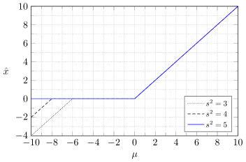
Figure 7: Solving (61) numerically for $a=0$ and $\gamma=1$.

We observe (and it can be proven) that for a given $\mu$ and $s^{2}$, and a sufficiently large $\gamma$, the estimate $\hat{x}$ is in $[a,\infty)$. More specifically, $\hat{x}\geq a$ is satisfied, if and only if

$$s^{2}\geq\begin{cases}0,&\text{if $\mu\geq a$}\\ \frac{|a-\mu|}{2\gamma},&\mathrm{else}.\end{cases}$$ (64)

Analogously, for a left-sided constraint, we have that $\hat{x}\leq a$ is satisfied, if and only if

$$s^{2}\geq\begin{cases}0,&\text{if $\mu\leq a$}\\ \frac{|a-\mu|}{2\gamma},&\mathrm{else}.\end{cases}$$ (65)

Note that since $\gamma$ is a free design parameter, (64) (or (65), respectively) can essentially always be satisfied.

V Applications

For the following application examples, we will employ the proposed prior models in larger Gaussian models, mostly based on an underlying state space model description of some physical model. Due to the recursive structure of the used state space models, the estimation of $x$ (or other state quantities) can efficiently be calculated for example by Gaussian message passing. For more details, the interested reader is referred to [9].

In general, we consider systems which evolve according to

$$x_{k} = Ax_{k-1}+Bu_{k},$$ (66)

$$y_{k} = Cx_{k}$$ (67)

where $k\in\{1,2,\ldots,K\}$, and where $A,B,C,x_{k},u_{k}$ and $y_{k}$ have appropriate dimensions.

V-A Box Constraints on Inputs

In the example of Fig. 8, the goal is to determine a bounded input sequence $u$ such that the system output $y$ approximates a given target trajectory $\breve{y}$ (i.e., $\|\breve{y}-y\|^{2}$ is minimized). The underlying linear system is a third-order low-pass filter (as in [9, Section 4.1]). To achieve this, a box constraint is applied on every input $u_{k}$, such that $u_{k}\in[-1,1]$, for $k\in\{1,\dots,K\}$.

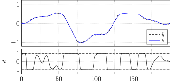
Figure 8: Box constraint on input enforcing $u\in[-1,1]^{K}$.

V-B Box Constraints on Outputs

In the example of Fig. 9, the goal is to determine a ternary input sequence $u$ (i.e., $u_{k}\in\{-1,0,1\}$) such that the system output $y$ lies in a predefined admissible corridor. The underlying linear system is a third-order low-pass filter. To achieve this, the corridor is modeled by applying box constraints on every output $y_{k}$, such that $y_{k}\in[a_{k},b_{k}]$, for $k\in\{1,\dots,K\}$, where $a_{k}$ and $b_{k}$ define the corridor at time instance $k$. The discrete-valued inputs are modeled by binary NUV priors as in [9].

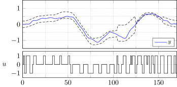
Figure 9: Box constraint on output enforcing $y$ to lie in a corridor. Input is $\{-1,0,1\}$-valued.

V-C Multiple Box Constraints on Outputs I

In the example of Fig. 10, the goal is to determine a ternary input sequence $u$ (i.e., $u_{k}\in\{-1,0,1\}$) such that the system output $y$ lies in either of two predefined admissible corridors. If the corridors intersect, the trajectory may switch the corridor, as can be seen in Fig. 10. The underlying linear system is a third-order low-pass filter. To achieve this, the two corridors are modeled as the sum of a binary shift variable $S_{k}\in\{0,d_{k}\}$ (modeled by a binary NUV prior [9]) and a box constraint, such that either $y_{k}\in[a_{k},b_{k}]$ or $y_{k}\in[a_{k}+d_{k},b_{k}+d_{k}]$, for $k\in\{1,\dots,K\}$. Note that $d_{k}$ is in general not constant. The prior model is given as factor graph in Fig. 11. The discrete-valued inputs are modeled by binary NUV priors as in [9].

Figure 10: Two admissible corridors can be realized by the sum of a binary decision variable and a box constraint on every output $y_{k}$. The input is $\{-1,0,1\}$-valued. The third plot indicates the “active” corridor ($c_{1}$ or $c_{2}$). The last plot illustrates the shift variable $s$.

Figure 11: Factor graph representing two shifted box constraints.

V-D Multiple Box Constraints on Outputs II (Flappy Bird)

In the example of Fig. 12, the goal is to “solve” a variation of the flappy bird computer game [14]. Consider an analog physical system consisting of a point mass $m$ moving forward (left to right in Fig. 12) with constant horizontal velocity and “falling” vertically with constant acceleration $g$. The $\{0,1\}$-valued control signal $u$ affects the system only if $u_{k}=1$, in which case a fixed value is added to the vertical momentum. We wish to steer the point mass such that it passes through the double slits, as illustrated in Fig. 12. To achieve this, the double slits are modeled as in Fig. 11, and the binary inputs are modeled by binary NUV priors as in [9]. The underlying dynamical system is given in [9, Section 4.2].

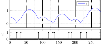
Figure 12: Flappy bird control with double-slit obstacles, binary control signal $u$, and resulting trajectory $y$.

V-E Half-Plane Constraints on Inputs

In the example of Fig. 13, the goal is to determine a lower-bounded input sequence $u$ such that the system output $y$ approximates a given target trajectory $\breve{y}$ (i.e., $\|\breve{y}-y\|^{2}$ is minimized). The underlying linear system is a third-order low-pass filter. To achieve this, a half-plane constraint is applied on every input $u_{k}$, such that $u_{k}\geq-1$, for $k\in\{1,\dots,K\}$.

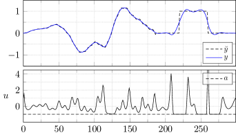
Figure 13: Half-space constraint on input enforcing $u_{k}\geq-1$.

V-F Convex Polyhedrons

Half-space constraints may be combined to define convex polyhedrons as admissible regions (see Fig. 16). The factor graph of such an prior model is given in Fig. 14, where the constraint is applied at the system output.

Figure 14: Prior model with convex polyhedron constraint, where $\tilde{Y}_{k}\in\mathbb{R}^{L}$ and where $p(\tilde{y}_{k})$ is the product of $L$ half-space priors.

The matrix $N_{k}$ projects the system output $y_{k}$ onto the normals of $L$ separating hyperplanes and is given by

$$N_{k}=\begin{bmatrix}n_{k,1}&n_{k,2}&\cdots&n_{k,L}\end{bmatrix}^{\mathsf{T}},$$ (68)

where each $n_{k,\ell}$ is a unity-length normal vector. The function $p(\tilde{y}_{k})$ is given by

$$p(\tilde{y}_{k})=\prod_{\ell=1}^{L}p(\tilde{y}_{k,\ell}),$$ (69)

where each $p(\tilde{y}_{k,\ell})$ is either a right- or left-sided half-plane constraint, centered around $a_{\ell}$. In Fig. 16 for example, we have $Y_{k}\in\mathbb{R}^{2}$, $L=3$ and

$$n_{k,1} = \begin{bmatrix}2\\ 3\end{bmatrix}/\sqrt{13},\quad$$ a_k,1 = 13 (70)

$$n_{k,2} = \begin{bmatrix}-1\\ 2\end{bmatrix}/\sqrt{5},\quad$$ a_k,2 = 5 (71)

$$n_{k,3} = \begin{bmatrix}0\\ 1\end{bmatrix},\quad$$ a_k,3 = 5, (72)

defining a triangle-shaped convex constraint. The resulting cost function is

$$\kappa(y_{k}) = \gamma\big{(}|n_{k,1}y_{k}-a_{k,1}|-(n_{k,1}y_{k}-a_{k,1})$$ (73)

$$+|n_{k,2}y_{k}-a_{k,2}|-(n_{k,2}y_{k}-a_{k,2})$$

$$+|n_{k,3}y_{k}-a_{k,3}|-(n_{k,3}y_{k}-a_{k,3})\big{)},$$

which is illustrated in Fig. 15.

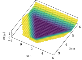
Figure 15: Cost function (73) for $\gamma=1$.

Figure 16: A convex polyhedron (in a two-dimensional setting) defined by three normal vectors.

In the example of Fig. 17, an object moves through a two-dimensional space. The goal is that at certain times, the object’s position must lie inside a convex admissible region, where each region is modeled by a combination of half-plane constraints, as explained above.

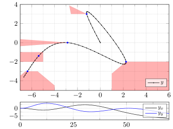
Figure 17: Convex polyhedron constraints modeled by multiple half-space constraints. The constraints enforce the blue points to be within the red convex polyhedrons.

V-G Reservoir-Balancing Problem

In this example, we consider a system of three interconnected water reservoirs, as illustrated in Fig. 18. Each reservoir has a maximum filling level ($V_{1}$, $V_{2}$ and $V_{3}$), which must not be exceeded. The goal of this example is to keep $V_{3}$ at a constant level of $\breve{V}_{3}=80$ (i.e., to minimize $\|V_{3}-\breve{V}_{3}\|^{2}$). To achieve this, water may be pumped between reservoirs, where each pump has a maximum achievable flow rate of $\Delta V_{1\rightarrow 2}\in[-1,1]$, $\Delta V_{1\rightarrow 3}\in[-1.5,2.5]$, and $\Delta V_{2\rightarrow 3}\in[-1,1.5]$. In addition, water from $V_{3}$ may be drained with flow rate $\Delta V_{3\rightarrow}\in[0,4]$. The observable disturbances $r_{1},r_{2}$ and $r_{3}$ (e.g., rain forecast) increase the filling levels in $V_{1}$, $V_{2}$ and $V_{3}$, respectively. The constraints on all filling levels and flow rates are box constraints and thus easily modeled by the proposed prior of Section III. Changing the flow rate of a pump (or valve) may be mechanically demanding; thus, we require changes in the flow rate to occur sparsely, by modeling them with sparsifying NUV priors [6]. Numerical results are give in Fig. 19. The bounds on all filling levels and flow rates are indicated by black dashed lines. The target level $\breve{V}_{3}$ is indicated by a blue dashed line in the third plot. It can be observed that at the time around $k=60$, the disturbance $r_{3}$ is compensated by draining and pumping water from the third reservoir to the first and the second. At around $k=140$, a slightly larger disturbance occurs which cannot be fully compensated by the other reservoirs, which leads to a significant swing in $V_{3}$.

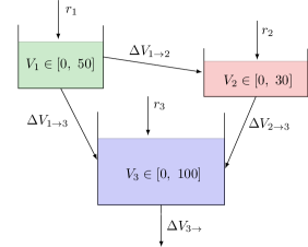
Figure 18: Three interconnected water reservoirs with filling levels $V_{1},V_{2}$ and $V_{3}$. The flow rates between reservoirs are indicated by $\Delta V_{(\cdot)}$.

Figure 19: Reservoir-balancing problem of three interconnected reservoirs. The filling levels are indicated by $V_{1},V_{2}$ and $V_{3}$. Water is pumped between the reservoirs to minimize $\|V_{3}-\breve{V}_{3}\|^{2}$, while keeping the number of changes in the flow rates sparse.

References

[1]
D. J. MacKay, “Bayesian interpolation,” Neural Comp., vol. 4, no. 3,
pp. 415–447, 1992.
[2]
M. E. Tipping, “Sparse Bayesian learning and the relevance vector machine,”
Journal of Machine Learning Research, vol. 1, pp. 211–244, 2001.
[3]
M. E. Tipping and A. C. Faul, “Fast marginal likelihood maximisation for
sparse Bayesian models,” in Proc. of the Ninth International Workshop
on Artificial Intelligence and Statistics, pp. 3–6, 2003.
[4]
D. P. Wipf and B. D. Rao, “Sparse Bayesian learning for basis selection,”
IEEE Trans. Signal Process., vol. 52, no. 8, pp. 2153–2164, 2004.
[5]
D. P. Wipf and S. S. Nagarajan, “A new view of automatic relevance
determination,” in Advances in Neural Information Processing Systems,
pp. 1625–1632, 2008.
[6]
H.-A. Loeliger, L. Bruderer, H. Malmberg, F. Wadehn, and N. Zalmai, “On
sparsity by NUV-EM, Gaussian message passing, and Kalman smoothing,”
in Information Theory and Applications Workshop (ITA), (La
Jolla, CA), pp. 1–10, 2016.
[7]
F. Bach, R. Jenatton, J. Mairal, and G. Obozinski, “Optimization with
sparsity-inducing penalties,” Foundations and Trends in Machine
Learning, vol. 4, no. 1, pp. 1–106, 2012.
[8]
H.-A. Loeliger, B. Ma, H. Malmberg, and F. Wadehn, “Factor graphs with NUV
priors and iteratively reweighted descent for sparse least squares and
more,” in Proc. Int. Symp. Turbo Codes & Iterative Inform. Process.
(ISTC), pp. 1–5, 2018.
[9]
R. Keusch, H. Malmberg, and H.-A. Loeliger, “Binary control and
digital-to-analog conversion using composite NUV priors and iterative
Gaussian message passing,” in IEEE International Conference on
Acoustics, Speech and Signal Processing (ICASSP), 2021.
[10]
R. Keusch and H.-A. Loeliger, “A binarizing NUV prior and its use for
M-level control and digital-to-analog conversion,” 2021.
[preprint arXiv:2105.02599].
[11]
R. H. Byrd and D. Payne, “Convergence of the iteratively reweighted least
squares algorithm for robust regression,” tech. rep., vol. 313, The Johns
Hopkins University, Baltimore, MD, 1979.
[12]
J. Schroeder, R. Yarlagadda, and J. Hershey, “Lp normed minimization with
applications to linear predictive modeling for sinusoidal frequency
estimation,” Signal Processing, vol. 24, no. 2, pp. 193–216, 1991.
[13]
H.-A. Loeliger, “An introduction to factor graphs,” IEEE Signal Process.
Mag., vol. 21, no. 1, pp. 28–41, 2004.