Active Ornstein-Uhlenbeck model for self-propelled particles with inertia

Abstract

Self-propelled particles, which convert energy into mechanical motion, exhibit inertia if they have a macroscopic size or move inside a gaseous medium, in contrast to micron-sized overdamped particles immersed in a viscous fluid. Here we study an extension of the active Ornstein-Uhlenbeck model, in which self-propulsion is described by colored noise, to access these inertial effects. We summarize and discuss analytical solutions of the particle’s mean-squared displacement and velocity autocorrelation function for several settings ranging from a free particle to various external influences, like a linear or harmonic potential and coupling to another particle via a harmonic spring. Taking into account the particular role of the initial particle velocity in a nonstationary setup, we observe all dynamical exponents between zero and four. After the typical intertial time, determined by the particle’s mass, the results inherently revert to the behavior of an overdamped particle with the exception of the harmonically confined systems, in which the overall displacement is enhanced by inertia. We further consider an underdamped model for an active particle with a time-dependent mass, which critically affects the displacement in the intermediate time-regime. Most strikingly, for a sufficiently large rate of mass accumulation, the particle’s motion is completely governed by inertial effects as it remains superdiffusive for all times.

I Introduction

The physics of self-propelled particles is a flourishing research arena. There exist many different biological microswimmers in nature, for instance, bacteria and unicellular protozoa, which typically generate their swimming motion with flagella or cilia powered by molecular motors Berg and Brown (1972); Machemer (1972). Janus particles are examples of synthetic microswimmers, which possess surfaces with two distinct physical or chemical properties. This asymmetric structure leads to self-propulsion via various mechanisms Walther and Muller (2013). Even on the single particle level, active motion is a nonequilibrium phenomenon, therefore challenging a basic modeling from a statistical mechanics point of view. In the last decades, various simple models were designed and proposed for single active particles including self-propulsion generated by nonlinear friction Fiasconaro et al. (2008); Romanczuk et al. (2012), by non-reciprocal bead motions Najafi and Golestanian (2004), and by an internal driving force combined with overdamped orientational Brownian dynamics Howse et al. (2007); Hagen et al. (2009); ten Hagen et al. (2011a), the latter leading to the standard model of active Brownian particles (ABPs) Bechinger et al. (2016).

More recently, the maybe simplest nontrivial model for an overdamped fluctuating self-propelled particle in a viscous fluid was proposed. Such an active Ornstein-Uhlenbeck particle (AOUP) possesses a stochastic driving force whose memory decays exponentially in time, leading to a persistence in the particle motion which mimicks the activity. This model, originally proposed by Ornstein and Uhlenbeck to study velocity distributions of passive particles Uhlenbeck and Ornstein (1930) and subsequently exploited for various other physical and mathematical problems Moss and McClintock (Eds.); Hänggi and Jung (1995); Masoliver and Porrà (1993); Łuczka (2005), has by now become a basic reference for active motion Fily and Marchetti (2012); Szamel et al. (2015); Sandford and Grosberg (2018); Solon et al. (2015); Fodor et al. (2016); Dabelow et al. (2019); Fily (2019); Caprini et al. (2019); Caprini and Marconi (2020a); Caprini et al. (2021); Bonilla (2019); Singh and Kundu (2021); Martin et al. (2021). Although the AOUP model does not resolve the orientational degrees of freedom, it admits some characteristic features of activity, like persistent motion, surface accumulation and, most prominently, motility-induced phase separation (MIPS) Fily and Marchetti (2012); Cates and Tailleur (2015). Describing self-propelled motion by an AOUP has the advantage that exact analytical solutions can be obtained for a large range of problems Szamel (2014); Das et al. (2018); Sandford et al. (2017); Marconi et al. (2017); Wittmann et al. (2018); Caprini et al. (2018); Caprini and Marconi (2020b). Moreover, the model provides a convenient basis to develop the theoretical description of more complex settings of interacting particles Marconi and Maggi (2015); Farage et al. (2015); Marconi et al. (2016); Wittmann and Brader (2016); Sharma et al. (2017); Wittmann et al. (2017a, b); Caprini and Marconi (2018); Wittmann et al. (2019). The experimental relevance of the AOUPs model has been also demonstrated for a passive tracer particle in an active bath Maggi et al. (2014, 2017).

If the self-propelled object has a macroscopic size or moves in a gaseous medium, the emerging inertial effects pose some new challenges for theoretical modeling. Depending on whether the motion is in a gas or a viscous medium, this underdamped active matter can be divided into two classes, namely ”dry” and ”wet” systems. Wet particles are affected by hydrodynamic effects, described within the Navier-Stokes equations Klotsa (2019), where the probably most prominent example from nature is a school of fish. In contrast, dry particles only perform a practically undamped motion due to their inertia. Apart from nature’s typical realization of such a system in a flock of birds, there is a large range of dry inertial particles whose motion is still affected by fluctuating random kicks of the surrounding medium. Whirling fruits self-propelling in the air Rabault et al. (2019) and small animals such as insects Mukundarajan et al. (2016); Devereux et al. (2021) are macroscopic examples found in nature. Besides these biological organisms, there are also artificial dry self-propelled particles. Mesoscopic dust particles in plasmas, the so-called ”complex plasma”, can be brought into a joint underdamped self-propulsion by nonreciprocal interactions Morfill and Ivlev (2009); Bartnick et al. (2016); Ivlev et al. (2015) or photophoresis Nosenko et al. (2020). Other examples of inertial dry active matter are man-made macroscopic granules self-propelling on a vibrating plate Narayan et al. (2007); Scholz et al. (2018a) or equipped with an internal vibration motor Dauchot and Démery (2019); Leoni et al. (2020) and mini-robots Mijalkov and Volpe (2013); Leyman et al. (2018). These various experimental realizations have also triggered an increasing number of theoretical work Scholz et al. (2018a); Debnath et al. (2020); Breoni et al. (2020); Sprenger et al. (2021); Gutierrez-Martinez and Sandoval (2020); Herrera and Sandoval (2021); Caprini and Marconi (2021a); Omar et al. (2021) considering dry active particles with inertia, see Löwen (2020) for a recent review.

In this paper, we study in detail the dynamical properties of an AOUP, whose translational motion is affected by inertia Puglisi and Marconi (2017); Caprini and Marconi (2021b). Our motivation for this choice is twofold. First, providing the simplest description of activity subject to inertia, the AOUP serves as a minimal reference model to compare and discuss experimental and simulation data. Second, it allows to understand inertial effects in various environments and settings through obtaining explicit analytical solutions. In detail, we give solutions for an inertial AOUP particle affected by constant and harmonic forces and then for two AOUPs connected by a harmonic spring. We further explore an active particle which ejects mass in an isotropic way. A graphical overview of these problems is given in Fig. 1 together with an illustration summarizing the different dynamical exponents obtained in this paper. Parts of our results have been independently obtained recently in Ref. Caprini and Marconi (2021b).

This paper is organized as follows. In Sec. II, we introduce the AOUP model and the dynamical quantities of interest. Then we present in Sec. III our main results, elaborating on the role of inertia and the effect of initial conditions, and conclude in Sec. IV.

II inertial AOUP model and noise averages

The active Ornstein-Uhlenbeck particle (AOUP) is arguably the simplest model for one self-propelled particle. It makes use of a stochastic driving velocity $\mathbf{u}(t)$ with a memory on a finite time scale $\tau$ leading to a persistent motion, which mimics activity. In detail, this Ornstein-Uhlenbeck process is defined by the stochastic equation

$$\dot{\mathbf{u}}(t)=-\frac{\mathbf{u}(t)}{\tau}+\frac{\bm{\xi}(t)}{\tau}\,,$$ (1)

where $\bm{\xi}(t)$ is a Gaussian distributed white noise, which is characterized by its first two moments, i.e. $\langle\xi_{i}(t)\rangle=0$ and $\langle\xi_{i}(t)\xi_{j}(t^{\prime})\rangle=2D\delta_{ij}\delta(t-t^{\prime})$ with $i,j\in\{1,...,d\}$ for $d$ spatial dimensions. Ornstein and Uhlenbeck originally developed the model to study the velocity distribution of passive particles Uhlenbeck and Ornstein (1930), but it can also be used for many other physical and mathematical problems. Solving Eq. (1) yields the moments for the random velocity $\mathbf{u}(t)$, which is Gaussian distributed colored noise, namely

$$\langle u_{i}(t)\rangle=0\quad\text{and}\quad\langle u_{i}(t)u_{j}(t^{\prime})\rangle=\frac{D}{\tau}\delta_{ij}{\rm e}^{-\frac{|t-t^{\prime}|}{\tau}}\,.$$ (2)

Here, $\tau$ is the persistence time, which is the time scale at which the stochastic self-propulsion velocity $\mathbf{u}(t)$ randomizes. The diffusion coefficient $D$ characterizes the motility of the particle. Both parameters describe the magnitude of the self-propulsion Wittmann et al. (2017a). The time scale of the AOUP is $\tau$, so a corresponding length scale can be defined as the persistence length $l_{0}\coloneqq\sqrt{D\tau}$. Finally, the active velocity

$$u_{0}:=\sqrt{\langle\mathbf{u}(t)\cdot\mathbf{u}(t)\rangle}=\sqrt{\frac{dD}{\tau}}$$ (3)

can be conveniently related to the equal-time self correlation of $\mathbf{u}(t)$, where $d$ is the spatial dimension. In the remainder of this work, we restrict ourselves to $d=2$.

The inertial dynamics can be described by the particle’s center-of-mass position $\mathbf{r}(t)$ and velocity $\dot{\mathbf{r}}(t)$. Given the initial conditions $\mathbf{r}_{0}:=\mathbf{r}(0)$ and $\dot{\mathbf{r}}_{0}:=\dot{\mathbf{r}}(0)$, we consider the underdamped equation of motion

$$m\ddot{\mathbf{r}}(t)+\gamma\dot{\mathbf{r}}(t)=\mathbf{F}_{\text{ext}}(\mathbf{r},t)+\gamma\mathbf{u}(t)$$ (4)

for one AOUP in the Langevin picture, where the coefficient of friction for linear drag is denoted by $\gamma$. Moreover, $\mathbf{F}_{\text{ext}}(\mathbf{r},t)=-\vec{\nabla}V_{\text{ext}}(\mathbf{r},t)$ is an external force caused by an external potential $V_{\text{ext}}(\mathbf{r},t)$ acting on the system and $\gamma\mathbf{u}(t)$ represents the active force. For a fixed activity of the AOUP, the inertial effects can be quantified by defining the dimensionless mass as

$$\tilde{m}\coloneqq\frac{m}{\gamma\tau}=\frac{\tau_{m}}{\tau}\,,$$ (5)

which can be written as a ratio of two basic time scales, namely the inertial delay time $\tau_{m}:=m/\gamma$ and the activity persistence time $\tau$.

As a Gaussian process the AOUP is characterized by its first two moments, Eq. (2), alone. To analyze the behavior of such a system, one can calculate dynamical averages and correlations. These are the velocity autocorrelation function (VACF)

$$V(t,t^{\prime}):=\langle\dot{\mathbf{r}}(t)\cdot\dot{\mathbf{r}}(t^{\prime})\rangle\,,$$ (6)

the mean displacement (MD)

$$\mathbf{X}(t):=\langle\mathbf{r}(t)-\mathbf{r}_{0}\rangle\,$$ (7)

and the mean-squared displacement (MSD)

$$\Delta(t):=\langle|\mathbf{r}(t)-\mathbf{r}_{0}|^{2}\rangle=2\int_{0}^{t}{\rm d}t_{1}\int_{0}^{t_{1}}{\rm d}t_{2}\,V(t_{1},t_{2})\,,$$ (8)

where the brackets $\langle\ldots\rangle$ denote a noise average as in Eq. (2). To characterize the dynamical behavior in different time regimes, we introduce the dynamical scaling exponent

$$\alpha(t):=\frac{\mathrm{d}\ln(\Delta(t))}{\mathrm{d}\ln(t)}\,,$$ (9)

of the MSD. We define the long-time self-diffusion coefficient as $D_{\text{L}}\coloneqq\lim_{t\to\infty}\frac{\Delta}{4t}$. This long-time limit exists in particular, if the dynamical scaling exponent tends to one as $t\to\infty$.

We finally remark that the second moments (MSD and VACF) are the same as for active Brownian particles upon identifying $u_{0}$ with a constant self-propulsion velocity in direction of the instantaneous orientation, subject to rotational diffusion with $D_{\text{r}}=\tau^{-1}$ Farage et al. (2015); Wittmann et al. (2017a) and neglecting translational Brownian diffusion. Note that, in the AOUP model, a passive Brownian system is conveniently obtained by taking the white-noise limit $\tau\rightarrow 0$ of zero persistence time $\tau$ in Eq. (1), such that the stochastic velocity $\mathbf{u}(t)\equiv\bm{\xi}(t)$ becomes a white noise with the (passive) diffusion coefficient $D$. For this reason, we do not include an additional white noise in Eq. (4) to represent the translational Brownian diffusion, usually present in the active Brownian case.

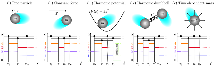
Figure 1: Overview of the main results. Top row: schematic illustration of an inertial active Ornstein-Uhlenbeck particle (AOUP) at position $\mathbf{r}(t)$ (gray sphere) and moving with velocity $\dot{\mathbf{r}}(t)$ (direction of the blue cloud). Its stochastic motion, determined by Eq. (4), depends on the initial conditions $\mathbf{r}_{0}:=\mathbf{r}(0)$ and $\dot{\mathbf{r}}_{0}:=\dot{\mathbf{r}}(0)$, its mass $m$, diffusion coefficient $D$, persistence time $\tau$ and the particular setup (i-v). Bottom row: qualitative illustration of the observed dynamical exponents $\alpha(t)$ (colored lines) in the mean-squared displacement (MSD). The relevant time regimes are drawn in different layers (upper horizontal bars). In each layer, the characteristic time scales (vertical bars with ticks on the $t$ axis) separating different regimes can be shifted horizontally (corresponding to a change of parameters), but their order is fixed (the big dots cannot get past each other). Shifting a solid vertical bar prolongs one adjacent time regime and shortens the other one or even completely overlays the regime(s) from the layer(s) below. The dashed vertical bar indicates the end of the inertial regime, which generally results in a fundamental change of the dynamical behavior. The exponents valid for the shown order of time scales are drawn as solid lines while the dotted lines become valid instead if the dashed vertical bar is shifted. The dotted vertical line indicates a transition between two distinct regimes with the same exponent. The annotated time scales correspond to the shown setting, while their full definition and meaning is explained in the text for each scenario. A detailed example of how to read this exponent diagram is given for a free particle in Sec. III.1.3. Columns: (i) force-free AOUP, cf. Sec. III.1, (ii) constant external force $\mathbf{F}$, cf. Sec. III.2, (iii) harmonic external potential with constant $k$ ($\alpha(t)$ is illustrated here for a spring with $k>0$), cf. Sec. III.3, (iv) two harmonically coupled AOUPs with equal mass $m$ but different diffusion coefficient $D^{\prime}$ and persistence time $\tau^{\prime}$ ($\alpha(t)$ is illustrated here for the center-of-mass coordinate $\mathbf{R}$), cf. Sec. III.4, and (v) with time-dependent mass $m(t)$ of constant slope $\dot{m}$ ($\alpha(t)$ is illustrated here for $\dot{m}<0$), cf. Sec. III.5.

III Results

In the following, we determine the solutions of the stochastic differential equation, Eq. (4) for both $\mathbf{r}(t)$ and $\dot{\mathbf{r}}(t)$ in the scenarios depicted in Fig. 1. Then, we calculate different correlation functions by carrying out the noise average with the help of Eq. (2) and discuss in detail the time- and mass dependence of the MSD. To provide the basis for our later study of a harmonic dumbbell and a free particle with linear mass ejection, we further elaborate on the known results Caprini and Marconi (2021b) for an AOUP in the absence of forces and in a harmonic potential. Moreover, we consider here a more general nonstationary setup of an AOUP with initial velocity $\dot{\mathbf{r}}_{0}$ and position $\mathbf{r}_{0}$ at time $t=0$. Selected full analytic solutions of the problems at hand are stated in Appendix A.

III.1 Free particle

As a basic reference, we first consider a free particle in the absence of any external forces $\mathbf{F}_{\text{ext}}=0$. The only relevant time scales which govern the dynamical correlations are the persistence time $\tau$ and the inertial delay time $\tau_{m}$.

III.1.1 Evaluation of analytic solutions

Solving the equation of motion for the velocity of a free particle, we find the general VACF as described in appendix A. Taking the steady-state limit, the VACF

$$\!\!\lim_{t^{\prime}\to\infty}V_{\text{f}}(t+t^{\prime},t^{\prime})=\frac{2\gamma^{2}D}{m^{2}-\gamma^{2}\tau^{2}}\left(\frac{m}{\gamma}{\rm e}^{-\gamma t/m}-\tau{\rm e}^{-t/\tau}\right)\!\!\!$$ (10)

decreases exponentially on the two time scales $\tau_{m}=m/\gamma$ and $\tau$, independent of the initial velocity $\dot{\mathbf{r}}_{0}$ Caprini and Marconi (2021b). The long-time mean-squared velocity

$$\lim_{t\to\infty}V_{\text{f}}(t,t)=\frac{2\gamma D}{m+\gamma\tau}=\frac{u_{0}^{2}}{\tilde{m}+1}$$ (11)

reflects that heavier particles have on average smaller absolute velocities than lightweight particles which is a clear manifestation of inertia. The MD

$$\mathbf{X}_{\text{f}}(t)=-\frac{m\dot{\mathbf{r}}_{0}}{\gamma}\left({\rm e}^{-\frac{\gamma t}{m}}-1\right)=\dot{\mathbf{r}}_{0}\,t+\mathcal{O}(t^{2})\,$$ (12)

does not depend on the activity since we consider here the stationary active velocity $\mathbf{u}(t)$ with the moments given by Eq. (2), lacking an initial direction. Instead, the MD reflects a persistent motion of particles with a finite initial velocity $\dot{\mathbf{r}}_{0}$ on the inertial time scale, i.e., for $t<\tau_{m}$. For later times, it takes a constant value $\lim_{t\to\infty}\mathbf{X}_{\text{f}}(t)=\frac{m\dot{\mathbf{r}}_{0}}{\gamma}$ determined by the magnitude and direction of $\dot{\mathbf{r}}_{0}$. This finding again constitutes a clear signature of inertia.

Now we turn to the MSD which we split as

$$\Delta_{\text{f}}(t)=\Delta^{\text{\!\!(ss)}}_{\text{f}}(t)+\Delta^{\text{\!\!(acc)}}_{\text{f}}(t)+\Delta^{\text{\!\!(0)}}_{\text{f}}(t)\,,$$ (13)

in terms of the stationary solution

$$\!\!\!\!\!\Delta^{\text{\!\!(ss)}}_{\text{f}}= \,\frac{4D\left[m^{3}\left({\rm e}^{-\frac{\gamma t}{m}}-1+\frac{\gamma t}{m}\right)-\gamma^{3}\tau^{3}\left({\rm e}^{-\frac{t}{\tau}}-1+\frac{t}{\tau}\right)\right]}{\gamma m^{2}-\gamma^{3}\tau^{2}}\!\!\!\!\!\!\!\!\!\!\!\!\!\!\!$$ (14)

$$= \,\frac{2\gamma D}{m+\gamma\tau}\,t^{2}-\frac{\gamma^{2}D}{6m\tau(m+\gamma\tau)}\,t^{4}+\mathcal{O}(t^{5})\!\!\!\!\!\!\!\!\!\!$$ (15)

for the MSD Caprini and Marconi (2021b), a correction term

$$\Delta^{\text{\!\!(acc)}}_{\text{f}}= -\frac{2mD\left({\rm e}^{-\frac{\gamma t}{m}}-1\right)}{\gamma m^{2}-\gamma^{3}\tau^{2}}\left[m(m+\gamma\tau)\left({\rm e}^{-\frac{\gamma t}{m}}-1\right)\right.\ \ \ \ \ \ \ \ \$$

$$\ \ \ \ \ \ \ \ \ \ \ \ \ \ \ \ \ \ \ \ \ \ \ \ \ \ \ \ \ \ \ \left.-2\gamma^{2}\tau^{2}\left({\rm e}^{-\frac{t}{\tau}}-1\right)\right]\ \ \ \ \ \ \ \ \$$

$$= -\frac{2\gamma D}{m+\gamma\tau}\,t^{2}+\frac{(3\gamma\tau+4m)\gamma^{2}D}{6m^{2}\tau(m+\gamma\tau)}\,t^{4}+\mathcal{O}(t^{5})\,,\!\!\!\!\!\!\!\!\!\!\!\!\!\!\!\!$$ (16)

initially decreasing the MSD to describe the acceleration of a massive particle starting from rest, and a purely inertial term

$$\Delta^{\text{\!\!(0)}}_{\text{f}}=\mathbf{X}_{\text{f}}\cdot\mathbf{X}_{\text{f}}= \,\frac{m^{2}\dot{\mathbf{r}}_{0}^{2}}{\gamma^{2}}\left({\rm e}^{-\frac{\gamma t}{m}}-1\right)^{2}$$ (17)

$$= \,\dot{\mathbf{r}}_{0}^{2}\,t^{2}-\frac{\gamma\dot{\mathbf{r}}_{0}^{2}}{m}\,t^{3}+\frac{7\gamma^{2}\dot{\mathbf{r}}_{0}^{2}}{12m^{2}}\,t^{4}+\mathcal{O}(t^{5})\,,\ \ \$$ (18)

reflecting the persistence of a general nonzero initial velocity $\dot{\mathbf{r}}_{0}$, just as the MD $\mathbf{X}_{\text{f}}$ stated in Eq. (12).

The two nonstationary contributions $\Delta^{\text{\!\!(acc)}}_{\text{f}}$ and $\Delta^{\text{\!\!(0)}}_{\text{f}}$ to the MSD vanish for zero mass and become constant after a long time. Therefore, both the overdamped limit

$$\lim_{m\to 0}\Delta_{\text{f}}=4D\tau\left({\rm e}^{-\frac{t}{\tau}}-1+\frac{t}{\tau}\right)=\frac{2D}{\tau}\,t^{2}-\frac{2D}{3\tau^{2}}\,t^{3}+\mathcal{O}(t^{4})$$ (19)

of the MSD and the long-time self-diffusion coefficient $D_{\text{L}}=D$ follow from $\Delta^{\text{\!\!(ss)}}_{\text{f}}$ alone. Hence, the diffusive behavior of a free inertial AOUP in the long-time limit is mass-independent, as also found for ABPs Scholz et al. (2018a). Since the quadratic terms in the short-time expansions of $\Delta^{\text{\!\!(ss)}}_{\text{f}}$ and $\Delta^{\text{\!\!(acc)}}_{\text{f}}$ cancel, the early behavior of the MSD is determined by $\Delta^{\text{\!\!(0)}}_{\text{f}}$ from Eq. (17). For an AOUP which is initially at rest, we find

$$\!\!\!\left.\Delta_{\text{f}}\right|_{\dot{\mathbf{r}}_{0}=\mathbf{0}}=\frac{\gamma^{2}D}{2\tau m^{2}}\,t^{4}-\frac{(5\gamma\tau+2m)\gamma^{2}D}{15\tau^{2}m^{3}}\,t^{5}+\mathcal{O}(t^{6})\,,$$ (20)

which means that it is accelerated on average by $\gamma u_{0}/m$, where $\gamma^{2}u_{0}^{2}$ is the average squared activity force. The corresponding expansion in the white-noise limit reads

$$\lim_{\tau\to 0}\left.\Delta_{\text{f}}\right|_{\dot{\mathbf{r}}_{0}=\mathbf{0}}= \,\frac{4\gamma^{2}D}{3m^{2}}\,t^{3}-\frac{\gamma^{3}D}{m^{3}}\,t^{4}+\mathcal{O}(t^{5})$$ (21)

and describes the motion of an initially resting passive particle Breoni et al. (2020).

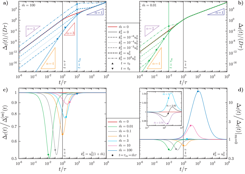
Figure 2: MSD $\Delta_{\text{f}}(t)$ of a free inertial AOUP, given by Eq. (13), with different initial velocities $\dot{\mathbf{r}}_{0}^{2}$ and masses $\tilde{m}=m/(\gamma\tau)$ (according to labels and legends) compared to the overdamped limit (thick red lines). The relevant time scales discussed in the text are highlighted (as labeled) where appropriate. a) MSD for fixed $m=100\gamma\tau$, such that $\tau_{m}>\tau$. b) MSD for fixed $m=0.01\gamma\tau$, such that $\tau_{m}<\tau$. c) MSD for fixed initial velocity $\dot{\mathbf{r}}_{0}^{2}=u_{0}^{2}/(1+\tilde{m})$, chosen to match the stationary mean-squared velocity, relative to the stationary MSD $\Delta^{\text{\!\!(ss)}}_{\text{f}}(t)$ given by Eq. (14). d) MSD for fixed $\dot{\mathbf{r}}_{0}^{2}=u_{0}^{2}$ relative to that in the overdamped limit, $m\rightarrow 0$, given by Eq. (19).

III.1.2 General discussion of the MSD

The MSD of a free AOUP is graphically evaluated in Fig. 2 for different parameters. Comparing both time scales involved, we observe two scenarios. First, if $\tau_{m}>\tau$ (or $\tilde{m}>1$, compare Fig. 2a), the onset of the long-time diffusive regime with $D_{\text{L}}=D$ occurs at $t>\tau_{m}$ and is thus delayed by inertial effects, when compared to the overdamped limit. Second, if $\tau_{m}<\tau$ (or $\tilde{m}<1$, compare Fig. 2b), there is a ballistic regime due to the persistent active motion for $\tau_{m}<t<\tau$ and the long-time diffusive regime is finally approached for $t>\tau$. More specifically, for $t>\tau_{m}$, the MSD generally behaves like in the overdamped limit, as given by Eq. (19).

As also shown in Figs. 2a and b, the behavior of the MSD in the early inertial regime for $t<\tau_{m}$ crucially depends on the ratio between the initial velocity $\dot{\mathbf{r}}_{0}$ and the long-time mean-squared velocity of the AOUP, given by Eq. (11), which indicates whether the AOUP must (on average) be accelerated or decelerated to reach the stationary state. For a sufficiently large $\dot{\mathbf{r}}_{0}^{2}\gtrsim u_{0}^{2}/(1+\tilde{m})$, the whole regime is governed by ballistic motion, according to Eq. (17). In the special case $\dot{\mathbf{r}}_{0}^{2}=u_{0}^{2}/(1+\tilde{m})$, the MSD closely follows that in the stationary state, as illustrated in Fig. 2c. The deviations around $t=\tau_{m}$, become negligible for a large mass. This can be understood from the short-time expansion in Eq. (14), and the fact that the MSD approaches overdamped behavior after the decay of inertial effects. If the initial velocity $\dot{\mathbf{r}}_{0}^{2}\lesssim u_{0}^{2}/(1+\tilde{m})$ is even smaller, the initial ballistic regime ends prematurely, as the AOUP is further accelerated.

To generally quantify the end of the initial ballistic regime, we introduce the time scale

$$\tau_{0}:=\min\left(2\tau_{m}\frac{|\dot{\mathbf{r}}_{0}|}{u_{0}},\tau_{m}\right),$$ (22)

which indicates the onset of an acceleration due to the average activity force and thus follows from equating the leading terms in the short-time expansions from Eq. (20) and Eq. (17), making use of the definition $u_{0}=\sqrt{2D/\tau}$. The corresponding superballistic regime with $\alpha=4$ is then observed in both Fig. 2a and Fig. 2b, for $\tau_{0}<t<\tau<\tau_{m}$ and $\tau_{0}<t<\tau_{m}<\tau$, respectively. In the former case, the exponent changes to $\alpha=3$, following Eq. (21), in the regime $\tau_{0}<\tau<t<\tau_{m}$, since the active velocity decorrelates at $t=\tau$. Moreover, if $\tau_{0}>\tau$, its role is taken by the alternative time scale

$$\tilde{\tau}_{0}:=\min\left(\frac{3\tau_{m}^{2}}{2\tau}\frac{\dot{\mathbf{r}}_{0}^{2}}{u_{0}^{2}},\tau_{m}\right),$$ (23)

deduced from Eq. (21) and Eq. (17). Then, for $\tau<\tilde{\tau}_{0}<t<\tau_{m}$, there is a direct transition from the initial ballistic regime to $\alpha=3$, as visible in Fig. 2a. If $\tau_{0}=\tau_{m}$ or $\tilde{\tau}_{0}=\tau_{m}$, there is no acceleration regime.

Finally, we consider the special case, $|\dot{\mathbf{r}}_{0}|=u_{0}$, that the absolute value of the initial velocity equals the active velocity. As highlighted in Fig. 2d, the MSD closely resembles the overdamped result for both $t\ll\tau_{m}$ and $t\gg\tau_{m}$, as the quadratic term in the respective short-time expansion from Eq. (17) and Eq. (19) is the same. The time- and mass-dependent deviation can be inferred from the cubic terms, which become equal for $m=3\gamma\tau$. For $m>3\gamma\tau$, we observe $\Delta_{\text{f}}\geq\lim_{m\rightarrow 0}\Delta_{\text{f}}$ for all times, which merely reflects the implied condition $\tau_{m}>\tau$, i.e., the ballistic regime due to the persistent initial velocity is longer than that due to persistent active motion in the overdamped limit, compare Fig. 2a. In contrast, for $m<3\gamma\tau$, the ratio $\Delta_{\text{f}}/\lim_{m\rightarrow 0}\Delta_{\text{f}}$ first decreases and then returns to unity when the inertial effects have fully relaxed, even if $\tau_{m}\geq\tau$. This behavior indicates that the initial velocity starts to decorrelate at an earlier time than the active motion. The same can be inferred for the whole duration of both decorrelation processes, regarding in Fig. 2d the situation for a mass slightly below $3\gamma\tau$. In the case $\tau_{m}<\tau$, where $\Delta_{\text{f}}\leq\lim_{m\rightarrow 0}\Delta_{\text{f}}$ for all times, we observe in Fig. 2b two ballistic regimes, separated at $t=\tau_{m}$, which both possess the same mean-squared velocity $u_{0}^{2}$ but for the two distinct physical reasons discussed before.

III.1.3 Summary and interpretation of the results

Our observations for a free AOUP are summarized in the first column of Fig. 1. This schematic exponent diagram should be understood as follows. The initial regime with $\alpha=2$ is always present (if $\tau_{0}>0$) and thus belongs to the uppermost layer. As we have $\tau_{0}\leq\tau_{m}$ per definition, these two time scales are drawn on the same layer Therefore, there are three possibilities for the subsequent dynamical regimes. First, if $\tau_{0}<\tau<\tau_{m}$, as depicted in the illustration, the sequence 2–4–3–1 of exponents $\alpha$ is given by the solid lines. Second, if $\tau<\tau_{0}<\tau_{m}$, which corresponds, e.g., to shifting the vertical bar for $\tau_{0}$ to the right, the regime for $t<\tau$ in the second layer indicating $\alpha=4$ is completely overlaid, such that the sequence is just 2–3–1. Third, if $\tau_{0}<\tau_{m}<\tau$, which corresponds, e.g., to shifting the vertical bar for $\tau_{m}$ to the left, the dotted lines between the old and new position of $\tau_{m}$ indicate the valid exponent, such that the sequence is 2–4–2–1. Further sequences are possible if two or more time scales are equal. In this qualitative picture $\tau_{0}$ generally represents the time at which the initial velocity ceases to be persistent. If one is interested in the explicit formula it should be read as either $\tau_{0}$ or $\tilde{\tau}_{0}$, depending on whether $\alpha$ changes to 3 or 4, as discussed in Sec. III.1.2.

Even in the most simplistic scenario without external forces, the MSD of an AOUP provides deep insights into the fundamental interplay of activity and inertia. In addition to the results apparent from Fig. 2, let us emphasize that the activity enters implicitly through the scaling factors $D$ and $\tau$. The effects of increasing the activity thus generally include (i) increasing values for the MSD, (ii) a delay of the onset of the diffusive regime and (iii) an effective reduction of the dimensionless mass $\tilde{m}$ (and thus of inertial effects in general), which should be kept in mind when regarding the following more complex scenarios.

III.2 Constant force

Next we consider the case of a constant external force ($\mathbf{F}_{\text{ext}}=\mathbf{F}$ with $F=|\mathbf{F}|$ in Eq. (4)). The steady-state VACF and mean-squared velocity only differ from the free-particle results stated in Eq. (10) and (11) by the constant term $F^{2}/\gamma^{2}$. The mean displacement $\mathbf{X}_{\text{c}}(t)$ can be written as

$$\mathbf{X}_{\text{c}}-\mathbf{X}_{\text{f}}=\frac{m\mathbf{F}}{\gamma^{2}}\left({\rm e}^{-\frac{\gamma t}{m}}-1+\frac{\gamma t}{m}\right)=\frac{\mathbf{F}}{2m}\,t^{2}+\mathcal{O}(t^{3})\,.$$ (24)

Hence, $\mathbf{X}_{\text{c}}$ deviates from the MD of a free particle given in Eq. (12) by a term which denotes an additional acceleration at short times and increases linearly in the long-time limit due to the directed linear force. As for a free particle, the pure MD does not carry a footprint of activity under our assumption of a stationary active velocity.

Likewise, the MSD $\Delta_{\text{c}}(t)$ of an AOUP in a constant force field is supplemented only by terms made up from activity-independent contributions that can be expressed in terms of the MD from Eq. (12) and Eq. (24)

$$\Delta_{\text{c}} -\Delta_{\text{f}}=\mathbf{X}_{\text{c}}\cdot\left(\mathbf{X}_{\text{c}}-\mathbf{X}_{\text{f}}\right)$$ (25)

$$=\dot{\mathbf{r}}_{0}\cdot\mathbf{F}\left(\frac{1}{2m}\,t^{3}-\frac{5\gamma}{12m^{2}}\,t^{4}\right)+\frac{F^{2}}{4m^{2}}\,t^{4}+\mathcal{O}(t^{5})\,.\ \ \ \ \ \$$ (26)

While these additional terms including the constant force $\mathbf{F}$ do not affect the MSD in the ballistic regime with persistent initial velocity $\dot{\mathbf{r}}_{0}$ for $t<\tau_{0}$, compare Eq. (17), the constant force further enhances the subsequent acceleration due to activity, which shortens the crossover time $\tau_{0}$ or $\tilde{\tau}_{0}$ compared to the values given in Eq. (22) or Eq. (23), respectively, for a free particle. Moreover, the dynamical exponent in the passive acceleration regime ($\tau<t<\tau_{m}$) may change from $\alpha=3$ according to Eq. (21) to $\alpha=4$ when Eq. (25) becomes dominant. Comparing these expansions, we predict that this happens at $\tau_{\text{c}}=16\gamma^{2}D/(3mF^{2}+12\gamma^{3}D)$ (if $\tau<\tau_{\text{c}}<\tau_{m}$). The long-time limit $\Delta_{\text{c}}\simeq(F^{2}/\gamma^{2})t^{2}$ of the MSD is always ballistic with velocity $F/\gamma$. This final regime surpasses a free-particle-like diffusive regime with $\Delta_{\text{c}}\simeq 4Dt$ for $t>\tilde{\tau}_{\text{c}}=4D\gamma^{2}/F^{2}$ if $\tilde{\tau}_{\text{c}}>\tau$ and $\tilde{\tau}_{\text{c}}>\tau_{m}$.

All possible dynamical exponents are illustrated in the second column of Fig. 1, where $\tau_{\text{c}}$ should be read as $\tilde{\tau}_{\text{c}}$ if the inertial time scale $\tau_{m}$ becomes shorter, as described above. We also see that in the case $\tau_{0}<\tau_{m}<\tau<\tilde{\tau}_{\text{c}}$ there are three distinct ballistic regimes due to persistent inertial motion with initial velocity $\dot{\mathbf{r}}_{0}$, persistent active motion and, finally, the constant external force.

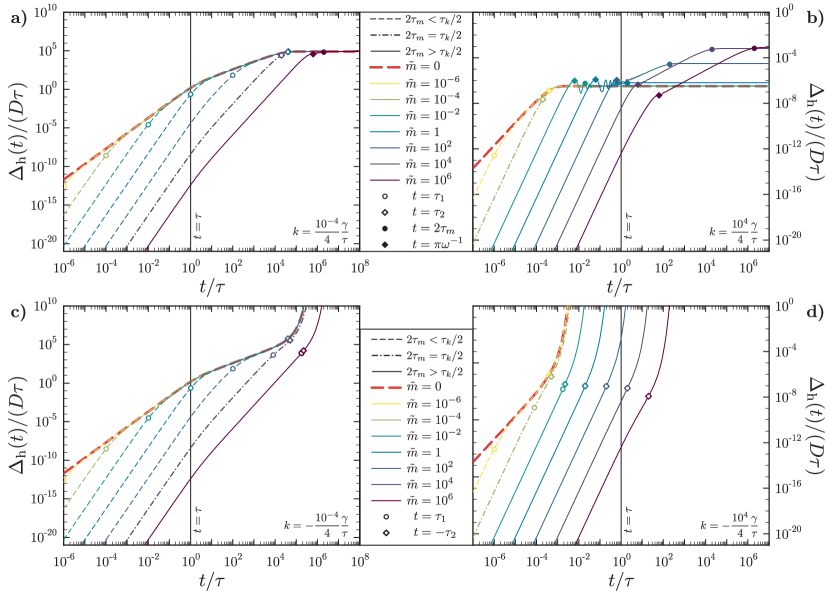
Figure 3: MSD of an inertial AOUP initially resting ($\dot{\mathbf{r}}_{0}=\mathbf{0}$) in the center ($\mathbf{r}_{0}=\mathbf{0}$) of a harmonic potential, Eq. (27), with constant $k$. We consider different masses $\tilde{m}=m/(\gamma\tau)$ (according to legends) and compare to the overdamped limit (thick red lines). a) MSD in a trap with $k=10^{-4}\gamma/(4\tau)$, such that $\tau_{k}>\tau$ and critical damping (dot-dashed lines) for $m=10^{4}\gamma\tau$. b) MSD in a trap with $k=10^{4}\gamma/(4\tau)$, such that $\tau_{k}<\tau$ and critical damping (dot-dashed lines) for $m=10^{-4}\gamma\tau$. c) MSD in an unstable potential with $k=-10^{-4}\gamma/(4\tau)$. d) MSD in an unstable potential with $k=-10^{4}\gamma/(4\tau)$.

III.3 Harmonic potential

As a next step we consider an AOUP subject to a time-independent external force in Eq. (4) generated by the harmonic potential

$$V_{\text{ext}}(\mathbf{r})=\frac{1}{2}k\mathbf{r}^{2}$$ (27)

with the constant $k$. We consider here both cases of a harmonic trap, where $k>0$ acts as a spring constant, and an unstable situation with $k<0$. For such a nonlinear potential the translational invariance is broken, such that the noise-averaged quantities of interest explicitly depend on the initial position $\mathbf{r}_{0}$.

Here we focus on the MSD $\Delta_{\text{h}}$, for which we obtain the general short-time expansion

$$\Delta_{\text{h}}(t)= \,\dot{\mathbf{r}}_{0}^{2}\,t^{2}-\frac{\dot{\mathbf{r}}_{0}\cdot(\gamma\dot{\mathbf{r}}_{0}+k\mathbf{r}_{0})}{m}\,t^{3}$$ (28)

$$+\frac{(7\gamma^{2}\dot{\mathbf{r}}_{0}^{2}-4km\dot{\mathbf{r}}_{0}^{2}+10\gamma k\mathbf{r}_{0}\cdot\dot{\mathbf{r}}_{0}+3k^{2}\mathbf{r}_{0}^{2})}{12m^{2}}\,t^{4}$$ (29)

$$+\frac{\gamma^{2}D}{2m^{2}\tau}\,t^{4}+\mathcal{O}(t^{5})\,,$$ (30)

whose leading terms with and without an initial velocity are the same as for a free particle, cf. Eq. (17) and Eq. (20), respectively. For vanishing initial conditions $\mathbf{r}_{0}=\mathbf{0}$ and $\dot{\mathbf{r}}_{0}=\mathbf{0}$, the first correction

$$\Delta_{\text{h}}(t)-\Delta_{\text{f}}(t)=-k\frac{\gamma^{2}D}{12m^{3}\tau}\,t^{6}+\mathcal{O}(t^{7})$$ (31)

to the free-particle expansion depending on $k$ appears at sixth order in time. The sign of this term indicates that the MSD compared to a free AOUP is reduced for a positive $k$, i.e., if the particle starts in the center of a harmonic trap, and enhanced for a negative $k$, i.e., if the particle initially sits on top of an unstable potential hill.

In the long-time limit, the MSD diverges exponentially for $k<0$, while we find for $k>0$ the expression

$$\lim_{t\to\infty}\Delta_{\text{h}}(t)=\mathbf{r}_{0}^{2}+\frac{2(m+\gamma\tau)\gamma D}{k(m+\gamma\tau+k\tau^{2})}\,,$$ (32)

which is constant in time and reflects how far (on average) the particle can climb the potential gradient of the trap. This distance thus increases (i) for an increasing average active velocity $u_{0}=\sqrt{2D/\tau}$, (ii) for an increasing persistence of the particle’s velocity due to inertia (increasing mass $m$) or activity (increasing persistence time $\tau$ at constant $u_{0}$) and (iii) for a decreasing spring constant $k$. The initial position of the particle in the potential merely marks a vertical offset.

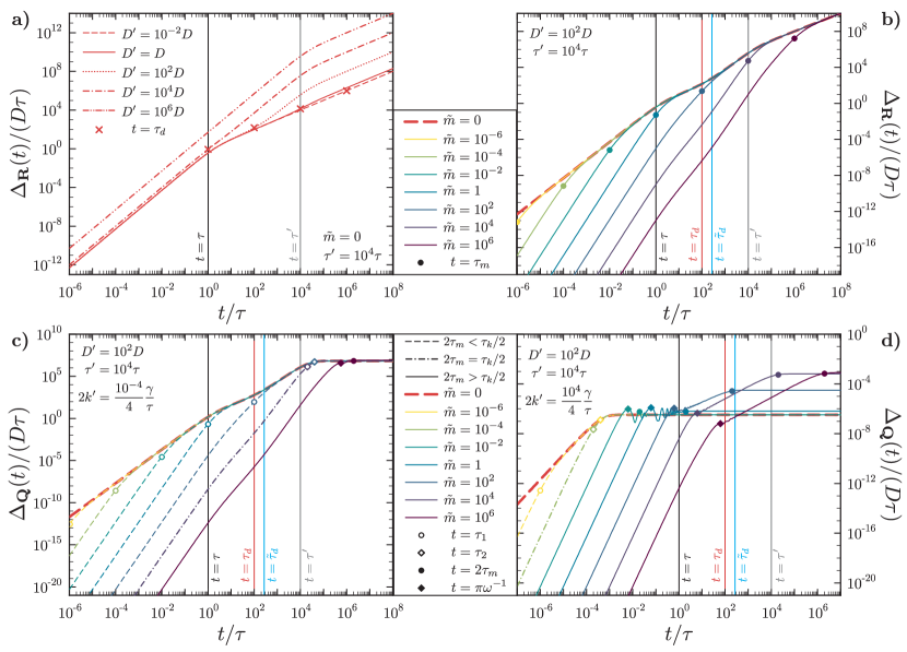
Figure 4: a,b) MSD $\Delta_{\mathbf{R}}$ of the center-of-mass coordinate $\mathbf{R}$ and c,d) MSD $\Delta_{\mathbf{Q}}$ of the relative coordinate $\mathbf{Q}$ for an inertial harmonic dumbbell consisting of two AOUPs, coupled by the spring constant $k^{\prime}$, with identical masses $\tilde{m}=m/(\gamma\tau)$ and zero initial velocity ($\dot{\mathbf{R}}_{0}=\dot{\mathbf{Q}}_{0}=\mathbf{0}$). The second particle may have a different persistence time $\tau^{\prime}$ and diffusivity $D^{\prime}$, which introduces two additional active time scales $\tau^{\prime}$ and $\tau_{\text{d}}$ (or $\tilde{\tau}_{\text{d}}$, see text for details), as indicated by the vertical lines. All parameter values are labeled or given in the legends.

To understand the full analytic solution for the MSD, given in appendix A and illustrated in Fig. 3, we first notice that in the overdamped limit the trap merely induces an additional time scale $\tau_{k}:=\gamma/|k|$, which indicates how long the particle can (on average) move freely before being affected by the potential. For a finite particle mass, the relevant passive time scales can be determined from the exponential solutions $\mathbf{r}(t)\propto\exp(-t/\tau_{1/2})$ of homogeneous differential equation $m\ddot{\mathbf{r}}(t)+\gamma\dot{\mathbf{r}}(t)+k\mathbf{r}(t)=\mathbf{0}$, while the active time scale $\tau$ enters through the inhomogeneous part of Eq. (4). In general, we find

$$\tau_{1/2}=\frac{2\tau_{m}}{1\pm\sqrt{1-4\frac{\tau_{m}}{\tau_{k}}\,\text{sgn}(k)}}\,,$$ (33)

where $\text{sgn}(k)$ denotes the sign of $k$. Expanding these factors for $\tau_{m}\ll\tau_{k}$ yields $\tau_{1}\simeq\tau_{m}$ and $\tau_{2}\simeq\text{sgn}(k)\tau_{k}$, which means that they denote the decay of inertial effects and the onset of potential effects, respectively. The detailed behavior depends on the sign of $k$ and is discussed in the following.

The MSD in a harmonic trap with $\text{sgn}(k)=1$ is illustrated in Figs. 3a and b. It becomes apparent that the different dynamical regimes are separated by the time scales $\tau$ and $\tau_{1/2}$ from Eq. (33) as long as the particle’s mass is below a critical value, determined by the condition $\tau_{k}/2=2\tau_{m}$, such that $\tau_{1}=\tau_{2}$. As long as $t\lesssim\tau_{2}$, the MSD resembles that discussed in Sec. III.1 for a free particle, which is best observed in Fig. 3a. Unlike the free-particle case, however, the MSD does not revert to the overdamped limit for $t\gg\tau_{1}$ but rather takes a constant value for long times, which explicitly depends on mass, activity and the spring constant, according to Eq. (32). For critical damping, the acceleration regime is directly followed by the final regime with a constant MSD. For even larger masses, we rewrite Eq. (33) as $\tau_{1/2}^{-1}=(2\tau_{m})^{-1}\pm i\omega$, introducing the angular frequency

$$\omega:=\frac{1}{2m}\sqrt{4km-\gamma^{2}}=\frac{1}{2\tau_{m}}\sqrt{4\frac{\tau_{m}}{\tau_{k}}-1}$$ (34)

of the oscillation, such that the MSD for $\dot{\mathbf{r}}_{0}=\mathbf{0}$ develops a first maximum after a half period $\pi\omega^{-1}$, compare Fig. 3b. The time scale $2\tau_{m}>\omega^{-1}$ then marks the end of the oscillatory regime in this underdamped case, as the inertial persistence ceases and the MSD remains constant.

The dynamical exponents of an overdamped AOUP in a harmonic trap are summarized in the third column of Fig. 1, where the indicated time scales represent the overdamped situation. In the underdamped case, where the time scale labeled as $\tau_{1}$ is larger than that labeled $\tau_{2}$, these labels should be interpreted as $\pi\omega^{-1}$ and $2\tau_{m}$, respectively. Further note that the active time scale $\tau$ does not indicate a change of the dynamical exponent if it is the longest time scale in the system but still affects the maximal MSD, given by Eq. (32), in the constant regime. In the most general scenario with $0<|\dot{\mathbf{r}}_{0}|<u_{0}$, $k>0$ and $\tau<\tau_{m}<\tau_{k}/4$, there are five different dynamical exponents $\alpha\in\{0,1,2,3,4\}$.

In the case of an unstable potential with $\text{sgn}(k)=-1$, there are always the two exponential time scales $\tau_{1}$ and $-\tau_{2}>\tau_{1}>0$ from Eq. (33). As shown in Figs. 3c and d, the MSD behaves like in the force-free case or in a harmonic trap until the particle begins to feel the potential at $t\approx-\tau_{2}$, which results in the onset of exponential growth. In contrast to the harmonic trap, the unstable potential has no critical damping. The equality of $\tau_{k}/2=2\tau_{m}$ rather indicates a crossover between the two limits $\tau_{m}\ll\tau_{k}$, where $-\tau_{2}\simeq\tau_{k}$ is mass-independent (and equal to the overdamped limit), and $\tau_{m}\gg\tau_{k}$, where $-\tau_{2}\simeq\tau_{1}\simeq\sqrt{\tau_{m}\tau_{k}}$ increases with increasing mass and approaches $\tau_{1}$.

III.4 Harmonic dumbbell

As a next step, we consider a generalization of Eq. (4) by introducing another AOUP with the same mass $m$ and an active velocity $\mathbf{u}^{\prime}(t)$ with the distinct parameters $D^{\prime}$ and $\tau^{\prime}$, which is coupled to the first particle by a harmonic force of spring constant $k^{\prime}>0$. The coupled Langevin equations describing this setup read

$$m\ddot{\mathbf{r}}_{1}+\gamma\dot{\mathbf{r}}_{1}+k^{\prime}(\mathbf{r}_{1}-\mathbf{r}_{2})=\gamma\mathbf{u}(t)\,,$$ (35)

$$m\ddot{\mathbf{r}}_{2}+\gamma\dot{\mathbf{r}}_{2}+k^{\prime}(\mathbf{r}_{2}-\mathbf{r}_{1})=\gamma\mathbf{u}^{\prime}(t)\,.$$ (36)

To decouple we transform the coordinates by defining the position of the center of mass as $\mathbf{R}(t)\coloneqq\frac{1}{2}(\mathbf{r}_{1}+\mathbf{r}_{2})$ and the relative position of the two particles as $\mathbf{Q}(t)\coloneqq\mathbf{r}_{1}-\mathbf{r}_{2}$. In these newly defined coordinates Eqs. (35) and (36) become

$$m\ddot{\mathbf{R}}+\gamma\dot{\mathbf{R}} =\frac{1}{2}(\mathbf{f}_{1}(t)+\mathbf{f}_{2}(t))\,,$$ (37)

$$m\ddot{\mathbf{Q}}+\gamma\dot{\mathbf{Q}}+2k^{\prime}\mathbf{Q} =\mathbf{f}_{1}(t)-\mathbf{f}_{2}(t)\,,$$ (38)

with the initial conditions ${\mathbf{R}}_{0}={\mathbf{R}}(0)$, $\dot{\mathbf{R}}_{0}=\dot{\mathbf{R}}(0)$, $\mathbf{Q}_{0}=\mathbf{Q}(0)$ and $\dot{\mathbf{Q}}_{0}=\dot{\mathbf{Q}}(0)$. In the following, we assume $\tau^{\prime}\geq\tau$ without loss of generality.

Focusing first on Eq. (37), we immediately see that the center of mass $\mathbf{R}$ behaves like a free particle subject to two independent random forces. The corresponding MSD can thus be constructed as

$$\left.\Delta_{\mathbf{R}}=\frac{\Delta_{\text{f}}+\Delta_{\text{f}}^{\prime}}{4}\right|_{\dot{\mathbf{r}}_{0}=2\dot{\mathbf{R}}_{0}}\,,$$ (39)

where $\Delta_{\text{f}}$ and $\Delta_{\text{f}}^{\prime}$ are both given by Eq. (13) for the respective activity parameters of the two particles. The center-of-mass motion is subject to the additional time scales $\tau_{\text{d}}:=D\tau^{\prime}/D^{\prime}$ and $\tau^{\prime}$, which is best understood in the overdamped limit. In this case, Fig. 4a illustrates that the initial ballistic motion for $t<\tau$, determined by the expansion $\Delta_{\mathbf{R}}=(D/\tau+D^{\prime}/\tau^{\prime})t^{2}+\mathcal{O}(t^{3})$, depends on the activity parameters of both particles. Likewise, we find $\Delta_{\mathbf{R}}\simeq(D+D^{\prime})t$ for $t>\tau^{\prime}$, which means that the value of the long-time diffusion coefficient $D_{\text{L}}=(D+D^{\prime})/4$ of the dumbbell equals half the average of that of two free particles. The MSD in the intermediate time regime, $\tau<t<\tau^{\prime}$, is subject to the competition between the diffusive behavior with $\Delta_{\mathbf{R}}\simeq Dt$ of the less persistent particle and the ballistic behavior with $\Delta_{\mathbf{R}}\simeq(D^{\prime}/\tau^{\prime})t^{2}$ of the more persistent particle. Equating the two expressions shows that a transition from the former to the latter can be observed at $t=\tau_{\text{d}}$ if $\tau<\tau_{\text{d}}<\tau^{\prime}$. Otherwise, there are in total only three time regimes, while in the two extreme cases $D^{\prime}\ll D$ and $D^{\prime}\gg D$ only the transition from ballistic to diffusive is observable at $t=\tau$ and $t=\tau^{\prime}$, respectively.

With inertia, the short-time behavior of the MSD differs from the overdamped limit for $t<\tau_{m}$, in analogy to a free particle. If the center of mass is initially at rest ($\dot{\mathbf{R}}_{0}=\mathbf{0}$), Fig. 4b illustrates up to three different superballistic acceleration regimes in the case $\tau<\tilde{\tau}_{\text{d}}<\tau_{m}$, where the time scale $\tilde{\tau}_{\text{d}}:=8D\tau^{\prime}/(3D^{\prime})$ for a possible transition from the dynamical exponent three to four can be found by equating the leading terms in Eq. (21) and Eq. (20) for the appropriate parameters. As $\tilde{\tau}_{\text{d}}\simeq{\tau}_{\text{d}}$, we observe in general analogy to the MSD of a free particle that the exponents three or four occur for $t<\tau_{m}$ if the overdamped behavior is diffusive or ballistic, respectively. All possible dynamical exponents are illustrated in the fourth column of Fig. 1, where $\tilde{\tau}_{\text{d}}$ takes the role $\tau_{\text{d}}$ if the inertial time scale $\tau_{m}$ becomes shorter, as described above.

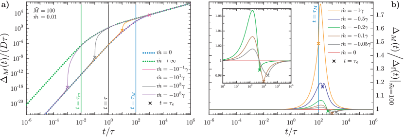
Figure 5: MSD of an inertial AOUP with vanishing initial velocity $\dot{\mathbf{r}}_{0}=\mathbf{0}$ and linear mass ejection $m(t)$, described by Eq. (41), from initial mass $M=100\gamma\tau$ to final mass $m=0.01\gamma\tau$ with different slopes $\dot{m}<0$ as labeled. The time $\tau_{\text{e}}$ at which the mass ejection ends is highlighted by crosses. a) Comparison to the MSD of a free particle with constant mass $m$ or $M$. b) Relative MSD to that of a free particle with mass $M$ for $\tau_{\text{e}}\simeq\tau_{M}$.

The relative position $\mathbf{Q}$ of the two monomers evolves in time according to Eq. (38), i.e., like a single particle in an effective harmonic trap with spring constant $k=2k^{\prime}$, compare Eq. (27). The resulting MSD can thus be expressed as

$$\left.\Delta_{\mathbf{Q}}=\left(\Delta_{\text{h}}+\Delta_{\text{h}}^{\prime}\right)\right|_{\dot{\mathbf{r}}_{0}=\dot{\mathbf{Q}}_{0}/2}\,,$$ (40)

where the full expression for $\Delta_{\text{h}}$ is given in appendix A. The relevant time scales $\tau_{1}^{\prime}$ and $\tau_{2}^{\prime}$, denoting the end of the inertial regime and the onset of confinement effects, respectively, can be inferred from Eq. (33). Recalling the discussion from Sec. III.3, the second active time scale $\tau^{\prime}$ is only relevant if it is not the largest time scale, which requires a relatively small (effective) coupling between the particles, as illustrated in Fig. 4c. In this case, the short-time behavior is similar (up to a factor four) to that of the unbounded center of mass with two active time scales, as discussed in the previous paragraph. The MSD then becomes constant for times exceeding the threshold which is set by the spring constant or the particles’ mass. The maximal displacement of the relative coordinate can be easily deduced from Eq. (32) and depends on all four activity coordinates and the particles’ mass. For a stronger coupling between the particles, Fig. 4d depicts characteristic oscillations in the relative MSD, whose angular frequency $\omega^{\prime}$ follows from inserting $k=2k^{\prime}$ into Eq. (33). In conclusion, there are up to seven different dynamical regimes possible for the relative position of the AOUPs connected to a harmonic dumbbell, covering all dynamical exponents $\alpha$ ranging from zero to four. This behavior can be illustrated by combining the third and fourth column of Fig. 1.

III.5 Time-dependent mass

Our final setup consists of a particle with a time-dependent mass $m(t)$. We consider here only an isotropic (undirected) ejection or accumulation of mass, in contrast to the rocket-like setup discussed in Ref. Sprenger et al. (2021). Hence, we start from the generic Langevin equation, Eq. (4), by replacing $m$ with $m(t)$ for a free particle with $\mathbf{F}_{\text{ext}}=0$. In particular, to allow for an analytic solution , we consider the mass to change linearly in time according to the function

$$m(t)=\begin{cases}M+\dot{m}t\,,\quad&\text{for }t<\frac{m-M}{\dot{m}}\,,\\ m\,,\quad&\text{for }t\geq\frac{m-M}{\dot{m}}\,,\end{cases}$$ (41)

where $M\coloneqq m(0)$ is the initial, $m$ the final mass of the particle and $\dot{m}$ denotes the constant time derivative of $m(t)$ in the time-dependent regime. The limits $\dot{m}\rightarrow 0$ and $\dot{m}\rightarrow\pm\infty$ correspond to a free AOUP with constant mass $M$ and $m$, respectively. Moreover, $\dot{m}<0$ denotes the rate of mass ejection and $\dot{m}>0$ the rate of mass accumulation. In the remainder of this section, we discuss the MSD $\Delta_{M}$ of an AOUP for these two cases separately.

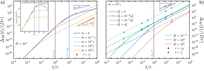
Figure 6: MSD of an inertial AOUP with linear mass accumulation $m(t)$ described by Eq. (41) with different slopes $\dot{m}>0$ as labeled. The time $\tau_{\text{e}}^{\prime}$ at which the gained mass $m(\tau_{\text{e}}^{\prime})-M=2M$ equals twice the initial mass $M$ is highlighted by crosses. a) Comparison for fixed initial mass $M=100\gamma\tau$ and vanishing initial velocity $\dot{\mathbf{r}}_{0}=\mathbf{0}$. The case $\dot{m}=0$ with constant mass $M$ corresponds to a free particle as in Fig. 2a. b) Comparison of the MSD with constant accumulation rate $\dot{m}=10^{3}\gamma$ for different initial parameters $M$ and $\dot{\mathbf{r}}_{0}^{2}$ as labeled. The lines corresponding to the same $\dot{\mathbf{r}}_{0}^{2}$ lie partially on top of each other.

III.5.1 Mass ejection

An AOUP whose mass decreases linearly in time according to Eq. (41) is affected by this process until all ”fuel” of mass $M-m$ is depleted at the characteristic time $\tau_{\text{e}}:=\frac{m-M}{\dot{m}}$. Afterwards it behaves as a free particle of mass $m$. Hence, for long times, the MSD generally reverts to the overdamped result. In terms of maximizing the MSD, the strategy to eject fuel gives a temporary advantage compared to moving with constant initial mass $M$ if the initial velocity $|\dot{\mathbf{r}}_{0}|\ll u_{0}$ is so small that the AOUP first needs to be accelerated, which we illustrate for an initially resting particle ($\dot{\mathbf{r}}_{0}=\mathbf{0}$) in Fig. 5a. The particular relevance of the possible inertial timescales $\tau_{M}=M/\gamma$ or $\tau_{m}=m/\gamma$ of the particle with or without fuel is therefore closely related to the time scale $\tau_{\text{e}}$ at which the change of mass takes effect.

In detail, for $\tau_{\text{e}}\gtrsim\tau_{M}$, i.e., a slow mass ejection, the overall MSD is largely the same as for a free AOUP with constant initial mass $M$, as the behavior for $t>\tau_{M}$ is not strongly affected by the particle’s mass. The behavior in this time regime is emphasized in Fig. 5b, which also illustrates the initially enhanced acceleration due to mass ejection. Moreover, the MSD for a sufficiently slow mass ejection eventually falls below the MSD for constant $M$, with a maximal relative deviation at $t=\tau_{\text{e}}$, which is because the velocity decorrelates earlier for a smaller mass $m(t)<M$, before the common overdamped limit is approached. For a faster mass ejection, the time scale $\tau_{\text{e}}$ indicates an exponential approach of the MSD to that of a free particle with mass $m$, as apparent from the nearly vertical lines in Fig. 5a. Hence, for $\tau_{m}\lesssim\tau_{\text{e}}\lesssim\tau_{M}$, the inertial regime ends abruptly at $t=\tau_{\text{e}}$, as the MSD directly switches from underdamped behavior with mass $M$ to the overdamped result. Finally, for $\tau_{\text{e}}\lesssim\tau_{m}$, there is a transition at $t=\tau_{\text{e}}$ between two different superballistic regimes with the same dynamical exponents, as the magnitude of the average acceleration decreases due to the lost mass. The inertial regime then ends at $t=\tau_{m}$.

The dynamical exponents for an AOUP with linear mass ejection are illustrated in the fifth column of Fig. 1, where the dotted vertical bar labeled $\tau_{\text{e}}$ is only relevant for $\tau_{\text{e}}<\tau_{m}$. If the time $\tau_{\text{e}}>\tau_{m}$ of mass ejection takes longer than the inertial time scale of the empty particle, then the label $\tau_{m}$ should be read as $\min\left(\tau_{\text{e}},\tau_{M}\right)$. This general exponent diagram also emphasizes that there is no effect of mass ejection observable (compared to a free particle with empty mass $m$) if the particle starts with a finite initial velocity $\dot{\mathbf{r}}_{0}$ such that $\tau_{0}>\tau_{\text{e}}$. This can be understood from the short-time expansion

$$\Delta^{\text{\!\!(0)}}_{M}=\,\dot{\mathbf{r}}_{0}^{2}\,t^{2}-\frac{\gamma\dot{\mathbf{r}}_{0}^{2}}{M}\,t^{3}+\frac{(7\gamma+4\dot{m})\gamma\dot{\mathbf{r}}_{0}^{2}}{12M^{2}}\,t^{4}+\mathcal{O}(t^{5})\,,$$ (42)

of the term depending on $\dot{\mathbf{r}}_{0}$, generalizing Eq. (17), whose leading order does not depend on the mass. Finally, we stress that for a large initial velocity $|\dot{\mathbf{r}}_{0}|\gg u_{0}$ the strategy of mass ejection results in a general disadvantage compared to moving with constant initial mass $M$, since the direction of $\dot{\mathbf{r}}_{0}$ remains persistent for a shorter time if the mass is depleted.

III.5.2 Mass accumulation

For an AOUP whose mass increases linearly over time according to Eq. (41), we focus on the particular limit $m\rightarrow\infty$ that the mass accumulation continues indefinitely. Next, we introduce the timescale $\tau_{\text{e}}^{\prime}:=\frac{2M}{\dot{m}}$ denoting the time when the particle has accumulated the double amount of its initial mass $M$ and examine its competition with the second inertial time scale $\tau_{M}=M/\gamma$. The typical behavior of the MSD is shown in Fig. 6a for an initially resting particle. The situation for a finite value of $m$ can be easily inferred by appreciating that the behavior reverts to the generic overdamped limit not later than $t=m/\gamma$, in analogy to earlier discussions. For $m\rightarrow\infty$, however, the MSD does not necessarily revert to overdamped behavior, as we discuss below.

In analogy to the ejection case, the MSD is qualitatively similar to that of a free AOUP with constant mass $M$ if $\tau_{\text{e}}^{\prime}\gtrsim\tau_{M}$, which means that the accumulation of mass happens not fast enough to delay or even prevent the end of the inertial regime. Thereafter, the particle’s motion does not become stationary, as its mean-squared velocity

$$V_{M}(t,t)\stackrel{{\scriptstyle t\gg\tau_{M}}}{{=}}\frac{2\gamma D}{m(t)+\gamma\tau}\ \ \ \ (\mbox{if}\ \tau_{\text{e}}^{\prime}>\tau_{M})$$ (43)

continuously decreases for long times, adiabatically following the free-particle result from Eq. (11). In the opposite case, for $\tau_{\text{e}}^{\prime}<\tau_{M}$, Fig. 6a shows that the slope of the MSD decreases as the particle becomes increasingly massive for $t\gtrsim\tau_{\text{e}}^{\prime}$, reflecting its retarded acceleration. The maximal velocity, once reached, then remains nearly persistent, as the acceleration due to random forces, which aim to disperse the particle’s direction of motion, becomes more and more irrelevant with increasing mass. This is best reflected in the particle’s mean-squared velocity $V_{m}(t,t)$, shown in the inset of Fig. 6a, for large rates $\dot{m}$ of mass accumulation. This balance eventually leads to superdiffusive but subballistic behavior in the long-time limit, i.e., the inertial regime never ends if $\tau_{\text{e}}^{\prime}<\tau_{M}$. The corresponding dynamical exponent

$$\alpha=2-\frac{\tau_{\text{e}}^{\prime}}{\tau_{M}}\ \ \ \ (\mbox{if}\ \tau_{\text{e}}^{\prime}<\tau_{M})\,,$$ (44)

can be determined analytically in the white-noise limit (which is generally recovered for $t\gg\tau$) and is numerically confirmed for all curves shown in Fig. 6. Therefore, the MSD for strong mass accumulation eventually surpasses that of an AOUP with $\tau_{\text{e}}^{\prime}>\tau_{M}$, which becomes diffusive ($\alpha=1$) at $t=\tau$ or $t=\tau_{M}$. In the special case $\tau_{\text{e}}^{\prime}=\tau_{M}$, the MSD behaves as $\Delta_{M}\simeq t\ln(t)$ for long times.

Apart from the modified dynamical exponent in Eq. (44), the long-time behavior in the case $\tau_{\text{e}}^{\prime}<\tau_{M}$ depends on both initial mass $M$ and velocity $\dot{\mathbf{r}}_{0}$, as illustrated in Fig. 6b, and (implicitly) also on the active velocity $u_{0}=\sqrt{2D/\tau}$. This observation is related to the particle’s maximal (persistent) velocity, which follows from these parameters. Therefore, the MSD at long times is generally enhanced for smaller $M$ and higher $u_{0}$, which both increase the initial acceleration as long as $|\dot{\mathbf{r}}_{0}|\lesssim u_{0}$. If (for $\tau_{\text{e}}^{\prime}<\tau_{M}$) the initial velocity $|\dot{\mathbf{r}}_{0}|\gtrsim u_{0}$ itself represents the maximal (persistent) velocity, the behavior of MSD is independent of the other parameters.

IV Conclusions

In conclusion, we have explored an active Ornstein-Uhlenbeck particle (AOUP) with inertia and calculated analytically various dynamical correlation functions such as the mean-square displacement (MSD). In particular, we extended recent work Caprini and Marconi (2021b) by including the explicit dependence on the initial velocity and by considering unstable inverted harmonic potentials, two coupled dumbbell-like particles and the situation of a time-dependent mass. Different dynamical scaling regimes were identified including power laws where the MSD scales in time $t$ with a power law $t^{\alpha}$. Here, the dynamical scaling exponent can be $\alpha\in\{0,1,2,3,4\}$. These scalings resemble results in other situations such as for an active Brownian particle (ABP) in a linear shear field ten Hagen et al. (2011b) or a disordered potential energy landscape Breoni et al. (2020).

In principle, our predictions can be tested in experiments on macroscopic self-propelled particles or mesoscopic particles in a gaseous background. Examples from the inanimate macroscopic world include vibration-driven granular particles Narayan et al. (2007); Kudrolli et al. (2008); Deseigne et al. (2010); Giomi et al. (2013); Weber et al. (2013); Klotsa et al. (2015); Patterson et al. (2017); Junot et al. (2017); Ramaswamy (2017); Deblais et al. (2018); Dauchot and Démery (2019), autorotating seeds and fruits Rabault et al. (2019); Fauli et al. (2019), camphor surfers Leoni et al. (2020), hexbug crawlers Leoni et al. (2020), trapped aerosols Di Leonardo et al. (2007) and mini-robots Rubenstein et al. (2014); Fujiwara et al. (2014); Tolba et al. (2015); Zhakypov et al. (2019); Yang et al. (2020). Another system which has gained more recent attention are complex plasmas consisting of mesoscopic charged dust particles Morfill and Ivlev (2009); Sütterlin et al. (2009); Couëdel et al. (2010); Chaudhuri et al. (2011); Ivlev et al. (2015); Nosenko et al. (2020); Lisin et al. (2020). Furthermore, animals moving at intermediate Reynolds number exhibit inertial effects such as swimming organisms like nematodes, brine shrimps or whirligig beetles Klotsa (2019); Devereux et al. (2021) and flying insects and birds Toner and Tu (1995, 1998); Chiappini (2008); Bartussek and Lehmann (2016); Mukundarajan et al. (2016); Bartussek and Lehmann (2018); Attanasi et al. (2014). Since, at low Reynolds numbers, a passive particle in a sea of active particles was shown to be an excellent realization of overdamped AOUP Maggi et al. (2014, 2017), one might expect that a macroscopic (inertial) passive particle in a background of other active particles will realize an inertial AOUP but this conjecture needs to be tested.

For the future, the inertial AOUP model can be extended to more complex situations. Among those is an inertial circle swimmer, a situation which has been explored for overdamped ABPs van Teeffelen and Löwen (2008); Kümmel et al. (2013); Löwen (2016) and overdamped AOUPs Caprini and Marconi (2019), and motions under an external magnetic field Vuijk et al. (2020); Abdoli and Sharma (2021) or in non-inertial frames Löwen (2019); Zheng and Löwen (2020). Last the collective behavior of many inertial active particles, such as MIPS Suma et al. (2014); Scholz et al. (2018b); Petrelli et al. (2018); Mayya et al. (2019); Mandal et al. (2019); Caprini and Marconi (2021a); Omar et al. (2021) or pattern formation in general Arold and Schmiedeberg (2020), is largely unexplored and our simple model may provide a stepping stone to access these fascinating phenomena.

Appendix A Additional and full analytic results

First, for a free particle, the general VACF

$$V_{\text{f}}(t_{1},t_{2})=\dot{\mathbf{r}}_{0}^{2}\,{\rm e}^{-\frac{\gamma(t_{1}+t_{2})}{m}}+\frac{2\gamma D}{m^{2}-\gamma^{2}\tau^{2}}$$ (45)

$$\ \ \cdot\bigg{\{}\gamma\tau\left({\rm e}^{-\frac{t_{1}}{\tau}-\frac{\gamma t_{2}}{m}}+{\rm e}^{-\frac{t_{2}}{\tau}-\frac{\gamma t_{1}}{m}}-{\rm e}^{-\frac{1}{\tau}(t_{1}-t_{2})}-{\rm e}^{-\frac{\gamma(t_{1}+t_{2})}{m}}\right)$$ (46)

$$\ \ \ \ \ +m\left({\rm e}^{-\frac{\gamma}{m}(t_{1}-t_{2})}-{\rm e}^{-\frac{\gamma}{m}(t_{1}+t_{2})}\right)\bigg{\}}\,,$$ (47)

calculated according to Eq. (6) and given here for the case $t_{1}\geq t_{2}$, does not only depend on the absolute difference $|t_{1}-t_{2}|$ because the system is not in steady-state. Taking the steady-state limit, $\lim_{t^{\prime}\to\infty}V_{\text{f}}(t^{\prime}+t,t^{\prime})$ yields the result stated in Eq. (10). The MSD, Eq. (13), is found from inserting the VACF from Eq. (47) into Eq. (8). In the steady state, the expression for the MSD reduces to Eq. (14), which can be seen by inserting the stationary VACF, Eq. (10), into Eq. (8).

Second, the full MSD for an AOUP in a harmonic potential, given by Eq. (27), is given by

$$\Delta_{\text{h}}(t)= \;\left[\left(\frac{\gamma\mathbf{r}_{0}}{2m}+\mathbf{v}_{0}\right)\frac{\sinh(\mu t)}{\mu}\,{\rm e}^{-\frac{\gamma t}{2m}}+\mathbf{r}_{0}\left(\cosh(\mu t)\,{\rm e}^{-\frac{\gamma t}{2m}}-1\right)\right]^{2}$$ (48)

$$+\frac{2D\gamma}{km(\gamma^{2}-4km)(m^{2}+2km\tau^{2}-\gamma^{2}\tau^{2}+k^{2}\tau^{4})}$$ (49)

$$\cdot\biggl{\{}-\gamma k\tau^{2}(\gamma^{2}-4km)\biggl{[}2m\tau\cosh(\mu t)+(2m+\gamma\tau)\frac{\sinh(\mu t)}{\mu}\biggr{]}{\rm e}^{-\left(\frac{\gamma}{2m}+\frac{1}{\tau}\right)t}$$ (50)

$$\ \ \ \ +m(m+\gamma\tau+k\tau^{2})\biggl{[}\frac{\gamma}{m}(\gamma^{2}-4km)(\gamma\tau-m)\cosh(\mu t)\,\frac{\sinh(\mu t)}{\mu}$$ (51)

$$\ \ \ \ \ \ \ \ \ \ \ \ \ \ \ \ \ \ \ \ \ \ \ \ \ \ \ \ \ \ \ \ +2\gamma(\gamma^{2}\tau-2km\tau-\gamma m)\cosh^{2}(\mu t)-\gamma^{3}\tau+\gamma^{2}m+4km^{2}\biggr{]}{\rm e}^{-\frac{\gamma t}{m}}$$

$$\ \ \ \ +m(\gamma^{2}-4km)(m+\gamma\tau)(m-\gamma\tau+k\tau^{2})\biggr{\}}\!\!\!\!\!\!\!$$ (52)

with $\mu\coloneqq\frac{\sqrt{1-4\frac{\tau_{m}}{\tau_{k}}\text{sgn}(k)}}{2\tau_{m}}=\frac{\sqrt{\gamma^{2}-4km}}{2m}$.

References

- Berg and Brown (1972) H. C. Berg and D. A. Brown, Nature 239, 500 (1972).
- Machemer (1972) H. Machemer, J. Exp. Biol. 57, 239 (1972).
- Walther and Muller (2013) A. Walther and A. H. Muller, Chem. Rev. 113, 5194 (2013).
- Fiasconaro et al. (2008) A. Fiasconaro, W. Ebeling, and E. Gudowska-Nowak, Eur. Phys. J. B 65, 403 (2008).
- Romanczuk et al. (2012) P. Romanczuk, M. Bär, W. Ebeling, B. Lindner, and L. Schimansky-Geier, Eur. Phys. J.: Spec. Top. 202 (2012).
- Najafi and Golestanian (2004) A. Najafi and R. Golestanian, Phys. Rev. E 69, 062901 (2004).
- Howse et al. (2007) J. R. Howse, R. A. Jones, A. J. Ryan, T. Gough, R. Vafabakhsh, and R. Golestanian, Phys. Rev. Lett. 99, 048102 (2007).
- Hagen et al. (2009) B. Hagen, S. van Teeffelen, and H. Löwen, Condens. Matter Phys. 12, 725 (2009).
- ten Hagen et al. (2011a) B. ten Hagen, S. van Teeffelen, and H. Löwen, J. Phys.: Condens. Matter 23, 194119 (2011a).
- Bechinger et al. (2016) C. Bechinger, R. Di Leonardo, H. Löwen, C. Reichhardt, G. Volpe, and G. Volpe, Rev. Mod. Phys. 88, 045006 (2016).
- Uhlenbeck and Ornstein (1930) G. E. Uhlenbeck and L. S. Ornstein, Phys. Rev. 36, 823 (1930).
- Moss and McClintock (Eds.) F. Moss and P. McClintock (Eds.), Noise in Nonlinear Dynamical Systems, Vol. 1 (Cambridge University Press, 1989).
- Hänggi and Jung (1995) P. Hänggi and P. Jung, Adv. Chem. Phys. 89, 239 (1995).
- Masoliver and Porrà (1993) J. Masoliver and J. M. Porrà, Phys. Rev. E 48, 4309 (1993).
- Łuczka (2005) J. Łuczka, Chaos 15, 026107 (2005).
- Fily and Marchetti (2012) Y. Fily and M. C. Marchetti, Phys. Rev. Lett. 108, 235702 (2012).
- Szamel et al. (2015) G. Szamel, E. Flenner, and L. Berthier, Phys. Rev. E 91, 062304 (2015).
- Sandford and Grosberg (2018) C. Sandford and A. Y. Grosberg, Phys. Rev. E 97, 012602 (2018).
- Solon et al. (2015) A. P. Solon, M. E. Cates, and J. Tailleur, Eur. Phys. J. Spec. Top. 224, 1231 (2015).
- Fodor et al. (2016) É. Fodor, C. Nardini, M. E. Cates, J. Tailleur, P. Visco, and F. van Wijland, Phys. Rev. Lett. 117, 038103 (2016).
- Dabelow et al. (2019) L. Dabelow, S. Bo, and R. Eichhorn, Phys. Rev. X 9, 021009 (2019).
- Fily (2019) Y. Fily, J. Chem. Phys. 150, 174906 (2019).
- Caprini et al. (2019) L. Caprini, U. M. B. Marconi, A. Puglisi, and A. Vulpiani, J. Stat. Mech.: Theory Exp. 2019, 053203 (2019).
- Caprini and Marconi (2020a) L. Caprini and U. M. B. Marconi, Phys. Rev. Res. 2, 033518 (2020a).
- Caprini et al. (2021) L. Caprini, A. Puglisi, and A. Sarracino, Symmetry 13 (2021).
- Bonilla (2019) L. L. Bonilla, Phys. Rev. E 100, 022601 (2019).
- Singh and Kundu (2021) P. Singh and A. Kundu, J. Phys. A: Math. Theor. 54, 305001 (2021).
- Martin et al. (2021) D. Martin, J. O’Byrne, M. E. Cates, E. Fodor, C. Nardini, J. Tailleur, and F. van Wijland, Phys. Rev. E 103, 032607 (2021).
- Cates and Tailleur (2015) M. E. Cates and J. Tailleur, Annu. Rev. Condens. Matter Phys. 6, 219 (2015).
- Szamel (2014) G. Szamel, Phys. Rev. E 90, 012111 (2014).
- Das et al. (2018) S. Das, G. Gompper, and R. G. Winkler, New J. Phys. 20, 015001 (2018).
- Sandford et al. (2017) C. Sandford, A. Y. Grosberg, and J.-F. Joanny, Phys. Rev. E 96, 052605 (2017).
- Marconi et al. (2017) U. M. B. Marconi, C. Maggi, and M. Paoluzzi, J. Chem. Phys. 147, 024903 (2017).
- Wittmann et al. (2018) R. Wittmann, J. M. Brader, A. Sharma, and U. M. B. Marconi, Phys. Rev. E 97, 012601 (2018).
- Caprini et al. (2018) L. Caprini, U. M. B. Marconi, and A. Vulpiani, J. Stat. Mech.: Theory Exp. 2018, 033203 (2018).
- Caprini and Marconi (2020b) L. Caprini and U. M. B. Marconi, Phys. Rev. Research 2, 033518 (2020b).
- Marconi and Maggi (2015) U. M. B. Marconi and C. Maggi, Soft Matter 11, 8768 (2015).
- Farage et al. (2015) T. F. F. Farage, P. Krinninger, and J. M. Brader, Phys. Rev. E 91, 042310 (2015).
- Marconi et al. (2016) U. M. B. Marconi, N. Gnan, M. Paoluzzi, C. Maggi, and R. Di Leonardo, Scientific Reports 6, 23297 (2016).
- Wittmann and Brader (2016) R. Wittmann and J. M. Brader, Europhysics Letters 114, 68004 (2016).
- Sharma et al. (2017) A. Sharma, R. Wittmann, and J. M. Brader, Phys. Rev. E 95, 012115 (2017).
- Wittmann et al. (2017a) R. Wittmann, C. Maggi, A. Sharma, A. Scacchi, J. M. Brader, and U. M. B. Marconi, J. Stat. Mech.: Theory Exp. 2017, 113207 (2017a).
- Wittmann et al. (2017b) R. Wittmann, U. M. B. Marconi, C. Maggi, and J. M. Brader, J. Stat. Mech.: Theory Exp. 2017, 113208 (2017b).
- Caprini and Marconi (2018) L. Caprini and U. M. B. Marconi, Soft Matter 14, 9044 (2018).
- Wittmann et al. (2019) R. Wittmann, F. Smallenburg, and J. M. Brader, J. Chem. Phys. 150, 174908 (2019).
- Maggi et al. (2014) C. Maggi, M. Paoluzzi, N. Pellicciotta, A. Lepore, L. Angelani, and R. Di Leonardo, Phys. Rev. Lett. 113, 238303 (2014).
- Maggi et al. (2017) C. Maggi, M. Paoluzzi, L. Angelani, and R. Di Leonardo, Scientific Reports 7, 17588 (2017).
- Klotsa (2019) D. Klotsa, Soft Matter 15, 8946 (2019).
- Rabault et al. (2019) J. Rabault, R. A. Fauli, and A. Carlson, Phys. Rev. Lett. 122, 024501 (2019).
- Mukundarajan et al. (2016) H. Mukundarajan, T. C. Bardon, D. H. Kim, and M. Prakash, J. Exp. Biol. 219, 752 (2016).
- Devereux et al. (2021) H. L. Devereux, C. R. Twomey, M. S. Turner, and S. Thutupalli, J. R. Soc. Interface 18, 20210114 (2021).
- Morfill and Ivlev (2009) G. E. Morfill and A. V. Ivlev, Rev. Mod. Phys. 81, 1353 (2009).
- Bartnick et al. (2016) J. Bartnick, A. Kaiser, H. Löwen, and A. V. Ivlev, J. Chem. Phys. 144, 224901 (2016).
- Ivlev et al. (2015) A. V. Ivlev, J. Bartnick, M. Heinen, C.-R. Du, V. Nosenko, and H. Löwen, Phys. Rev. X 5, 011035 (2015).
- Nosenko et al. (2020) V. Nosenko, F. Luoni, A. Kaouk, M. Rubin-Zuzic, and H. Thomas, Phys. Rev. Res. 2, 033226 (2020).
- Narayan et al. (2007) V. Narayan, S. Ramaswamy, and N. Menon, Science 317, 105 (2007).
- Scholz et al. (2018a) C. Scholz, S. Jahanshahi, A. Ldov, and H. Löwen, Nat. Commun. 9, 5156 (2018a).
- Dauchot and Démery (2019) O. Dauchot and V. Démery, Phys. Rev. Lett. 122, 068002 (2019).
- Leoni et al. (2020) M. Leoni, M. Paoluzzi, S. Eldeen, A. Estrada, L. Nguyen, M. Alexandrescu, K. Sherb, and W. W. Ahmed, Phys. Rev. Res. 2, 043299 (2020).
- Mijalkov and Volpe (2013) M. Mijalkov and G. Volpe, Soft Matter 9, 6376 (2013).
- Leyman et al. (2018) M. Leyman, F. Ogemark, J. Wehr, and G. Volpe, Phys. Rev. E 98, 052606 (2018).
- Debnath et al. (2020) D. Debnath, P. K. Ghosh, V. R. Misko, Y. Li, F. Marchesoni, and F. Nori, Nanoscale 12, 9717 (2020).
- Breoni et al. (2020) D. Breoni, M. Schmiedeberg, and H. Löwen, Phys. Rev. E 102, 062604 (2020).
- Sprenger et al. (2021) A. R. Sprenger, S. Jahanshahi, A. V. Ivlev, and H. Löwen, Phys. Rev. E 103, 042601 (2021).
- Gutierrez-Martinez and Sandoval (2020) L. L. Gutierrez-Martinez and M. Sandoval, J. Chem. Phys. 153, 044906 (2020).
- Herrera and Sandoval (2021) P. Herrera and M. Sandoval, Phys. Rev. E 103, 012601 (2021).
- Caprini and Marconi (2021a) L. Caprini and U. M. B. Marconi, Soft Matter 17, 4109 (2021a).
- Omar et al. (2021) A. K. Omar, K. Klymko, T. GrandPre, P. L. Geissler, and J. F. Brady, arXiv:2108.10278 (2021).
- Löwen (2020) H. Löwen, J. Chem. Phys. 152, 040901 (2020).
- Puglisi and Marconi (2017) A. Puglisi and U. M. B. Marconi, Entropy 19, 356 (2017).
- Caprini and Marconi (2021b) L. Caprini and U. M. B. Marconi, J. Chem. Phys. 154, 024902 (2021b).
- Note (1) The problem of an AOUP with a time-dependent mass as given by Eq. (41\@@italiccorr) admits an analytic solution for the MSD in terms of hypergeometric functions, which is too lengthy to be stated here but is available from the authors upon request.
- ten Hagen et al. (2011b) B. ten Hagen, R. Wittkowski, and H. Löwen, Phys. Rev. E 84, 031105 (2011b).
- Kudrolli et al. (2008) A. Kudrolli, G. Lumay, D. Volfson, and L. S. Tsimring, Phys. Rev. Lett. 100, 058001 (2008).
- Deseigne et al. (2010) J. Deseigne, O. Dauchot, and H. Chaté, Phys. Rev. Lett. 105, 098001 (2010).
- Giomi et al. (2013) L. Giomi, N. Hawley-Weld, and L. Mahadevan, Proc. Royal Soc. A 469, 20120637 (2013).
- Weber et al. (2013) C. A. Weber, T. Hanke, J. Deseigne, S. Léonard, O. Dauchot, E. Frey, and H. Chaté, Phys. Rev. Lett. 110, 208001 (2013).
- Klotsa et al. (2015) D. Klotsa, K. A. Baldwin, R. J. A. Hill, R. M. Bowley, and M. R. Swift, Phys. Rev. Lett. 115, 248102 (2015).
- Patterson et al. (2017) G. A. Patterson, P. I. Fierens, F. Sangiuliano Jimka, P. G. König, A. Garcimartín, I. Zuriguel, L. A. Pugnaloni, and D. R. Parisi, Phys. Rev. Lett. 119, 248301 (2017).
- Junot et al. (2017) G. Junot, G. Briand, R. Ledesma-Alonso, and O. Dauchot, Phys. Rev. Lett. 119, 028002 (2017).
- Ramaswamy (2017) S. Ramaswamy, J. Stat. Mech.: Theory Exp. 2017, 054002 (2017).
- Deblais et al. (2018) A. Deblais, T. Barois, T. Guerin, P. H. Delville, R. Vaudaine, J. S. Lintuvuori, J. F. Boudet, J. C. Baret, and H. Kellay, Phys. Rev. Lett. 120, 188002 (2018).
- Fauli et al. (2019) R. A. Fauli, J. Rabault, and A. Carlson, Phys. Rev. E 100, 013108 (2019).
- Di Leonardo et al. (2007) R. Di Leonardo, G. Ruocco, J. Leach, M. J. Padgett, A. J. Wright, J. M. Girkin, D. R. Burnham, and D. McGloin, Phys. Rev. Lett. 99, 010601 (2007).
- Rubenstein et al. (2014) M. Rubenstein, A. Cornejo, and R. Nagpal, Science 345, 795 (2014).
- Fujiwara et al. (2014) R. Fujiwara, T. Kano, and A. Ishiguro, Advanced Robotics 28, 639 (2014).
- Tolba et al. (2015) S. Tolba, R. Ammar, and S. Rajasekaran, in IEEE Symposium on Computers and Communication (ISCC) (IEEE, 2015) pp. 1007–1013.
- Zhakypov et al. (2019) Z. Zhakypov, K. Mori, K. Hosoda, and J. Paik, Nature 571, 381 (2019).
- Yang et al. (2020) X. Yang, C. Ren, K. Cheng, and H. P. Zhang, Phys. Rev. E 101, 022603 (2020).
- Sütterlin et al. (2009) K. R. Sütterlin, A. Wysocki, A. V. Ivlev, C. Räth, H. M. Thomas, M. Rubin-Zuzic, W. J. Goedheer, V. E. Fortov, A. M. Lipaev, V. I. Molotkov, O. F. Petrov, G. E. Morfill, and H. Löwen, Phys. Rev. Lett. 102, 085003 (2009).
- Couëdel et al. (2010) L. Couëdel, V. Nosenko, A. V. Ivlev, S. K. Zhdanov, H. M. Thomas, and G. E. Morfill, Phys. Rev. Lett. 104, 195001 (2010).
- Chaudhuri et al. (2011) M. Chaudhuri, A. V. Ivlev, S. A. Khrapak, H. M. Thomas, and G. E. Morfill, Soft Matter 7, 1287 (2011).
- Lisin et al. (2020) E. A. Lisin, O. F. Petrov, E. A. Sametov, O. S. Vaulina, K. B. Statsenko, M. M. Vasiliev, J. Carmona-Reyes, and T. W. Hyde, Scientific Reports 10, 13653 (2020).
- Toner and Tu (1995) J. Toner and Y. Tu, Phys. Rev. Lett. 75, 4326 (1995).
- Toner and Tu (1998) J. Toner and Y. Tu, Phys. Rev. E 58, 4828 (1998).
- Chiappini (2008) E. Chiappini, Encyclopedia of Entomology (Springer Netherlands, 2008) pp. 152–154.
- Bartussek and Lehmann (2016) J. Bartussek and F. O. Lehmann, Royal Soc. Open Sci. 3, 150562 (2016).
- Bartussek and Lehmann (2018) J. Bartussek and F. O. Lehmann, J. Royal Soc. Interface 15, 20180408 (2018).
- Attanasi et al. (2014) A. Attanasi, A. Cavagna, L. Del Castello, I. Giardina, T. S. Grigera, A. Jelic, S. Melillo, L. Parisi, O. Pohl, E. Shen, and M. Viale, Nat. Phys. 10, 692 (2014).
- van Teeffelen and Löwen (2008) S. van Teeffelen and H. Löwen, Phys. Rev. E 78, 020101 (2008).
- Kümmel et al. (2013) F. Kümmel, B. ten Hagen, R. Wittkowski, I. Buttinoni, R. Eichhorn, G. Volpe, H. Löwen, and C. Bechinger, Phys. Rev. Lett. 110, 198302 (2013).
- Löwen (2016) H. Löwen, Eur. Phys. J.: Spec. Top. 225, 2319 (2016).
- Caprini and Marconi (2019) L. Caprini and U. M. B. Marconi, Soft Matter 15, 2627 (2019).
- Vuijk et al. (2020) H. D. Vuijk, J. U. Sommer, H. Merlitz, J. M. Brader, and A. Sharma, Phys. Rev. Res. 2, 013320 (2020).
- Abdoli and Sharma (2021) I. Abdoli and A. Sharma, Soft Matter 17, 1307 (2021).
- Löwen (2019) H. Löwen, Phys. Rev. E 99, 062608 (2019).
- Zheng and Löwen (2020) Y. Zheng and H. Löwen, Phys. Rev. Res. 2, 023079 (2020).
- Suma et al. (2014) A. Suma, G. Gonnella, D. Marenduzzo, and E. Orlandini, Europhysics Letters 108, 56004 (2014).
- Scholz et al. (2018b) C. Scholz, M. Engel, and T. Pöschel, Nat. Commun. 9, 931 (2018b).
- Petrelli et al. (2018) I. Petrelli, P. Digregorio, L. F. Cugliandolo, G. Gonnella, and A. Suma, Eur. Phys. J. E 41, 128 (2018).
- Mayya et al. (2019) S. Mayya, G. Notomista, D. Shell, S. Hutchinson, and M. Egerstedt, in 2019 IEEE/RSJ International Conference on Intelligent Robots and Systems (IROS) (2019) pp. 4106–4112.
- Mandal et al. (2019) S. Mandal, B. Liebchen, and H. Löwen, Phys. Rev. Lett. 123, 228001 (2019).
- Arold and Schmiedeberg (2020) D. Arold and M. Schmiedeberg, J. Phys.: Condens. Matter 32, 315403 (2020).