Uniform Consistency in Nonparametric Mixture Models

Abstract

We study uniform consistency in nonparametric mixture models as well as closely related mixture of regression (also known as mixed regression) models, where the regression functions are allowed to be nonparametric and the error distributions are assumed to be convolutions of a Gaussian density. We construct uniformly consistent estimators under general conditions while simultaneously highlighting several pain points in extending existing pointwise consistency results to uniform results. The resulting analysis turns out to be nontrivial, and several novel technical tools are developed along the way. In the case of mixed regression, we prove $L^{1}$ convergence of the regression functions while allowing for the component regression functions to intersect arbitrarily often, which presents additional technical challenges. We also consider generalizations to general (i.e., non-convolutional) nonparametric mixtures.

1 Introduction

Mixture models are a classical approach to modeling heterogeneous populations composed of many subpopulations, and have found a variety of applications in prediction and classification (Castelli and Cover, 1995, 1996; Cozman et al., 2003; Dan et al., 2018), clustering (Fraley and Raftery, 2002; Melnykov and Maitra, 2010), and latent variable models (Allman et al., 2009; Gassiat et al., 2020; Kivva et al., 2021, 2022). Mixture models can also be used as a flexible tool for density estimation (Genovese and Wasserman, 2000; Ghosal and Van Der Vaart, 2007; Kruijer et al., 2010) and arise in the study of empirical Bayes (Saha and Guntuboyina, 2020; Feng and Dicker, 2018) and deconvolution (Fan, 1991; Zhang, 1990; Moulines et al., 1997). When covariates are involved, mixtures can be used to model heterogeneous dependencies between an observation $Y$ and some covariate(s) $X$, in which the conditional distribution $\mathbb{P}[Y\,|\,X=x]$ arises as a mixture of multiple (noisy) regression curves. Despite their relevance and usefulness in applications, mixture models can be notoriously difficult to analyze: Except in special cases, mixture models are a classical example of a nonidentifiable, irregular statistical model. As one might imagine, this situation is exacerbated for nonparametric mixtures, to the extent that even fundamental properties such as identifiability and consistency remain only partially addressed.

For parametric mixture models, many of these issues have been carefully addressed: We now have optimal estimators for Gaussian mixtures (Heinrich and Kahn, 2018; Wu and Yang, 2020; Doss et al., 2020), a detailed understanding of the EM algorithm for mixtures (Balakrishnan et al., 2017; Cai et al., 2019), and efficient algorithms for mixed linear regression models (Yi et al., 2014; Kwon et al., 2021). The situation for nonparametric mixtures, however, is quite different. Here and in the sequel, by a “nonparametric mixture” we mean a finite mixture whose mixture components belong to a nonparametric family of distributions. For both vanilla nonparametric mixtures and mixtures of nonparametric regressions, much less is known despite many decades of work. For example, although there is a substantial body of work focused on core identifiability and estimation problems, uniform consistency has been comparatively understudied; see Section 2 for a more detailed review of previous work.

Motivated by this disparity, in this paper we study uniform consistency in nonparametric mixture models and highlight several subtleties that arise when constructing uniformly consistent estimators and that appear to be peculiar to the setting of nonparametric mixtures. Although uniform consistency is often an afterthought—typically amounting to compactness and uniformity assumptions on the model—we hope to illustrate that for nonparametric mixtures, uniform consistency is a subtle matter with some surprising properties. By “uniform consistency” we mean consistency that is uniform over a statistical model. We will focus on the nonparametric generalization of mixed regression, in which $\mathbb{P}[Y\,|\,X=x]$ is a mixture over $K$ nonparametric regression models $m_{k}(x)+z_{k}$, where the error distribution is assumed to be unknown and comes from a nonparametric family of densities. As a special case, this subsumes vanilla nonparametric mixtures (i.e., without covariates), which will be considered as well.

Let us begin by introducing the statistical model that will be our primary interest (for technical definitions, see Section 3): The response $Y$ is modeled by $m_{k}(X)+z_{k}$ with probability $\lambda_{k}$ ($k=1,\ldots,K$) and $z_{k}\sim f$, where $m_{k}$ are regression functions, $f$ is a density function, and $\lambda_{k}$ are weights satisfying $0<\lambda_{k}<1$ and $\sum_{k}\lambda_{k}=1$. Assuming as usual that the noise $z_{k}$ is independent of the covariates $X$, this implies that the conditional density $p(\,\cdot\,|\,x)$ satisfies

$$p(y\,|\,x)=\sum_{k}\lambda_{k}f(y-m_{k}(x)).$$ (1)

In other words, for each fixed $x$, we have a mixture model whose weights and components are given by $\lambda_{k}$ and $f(y-m_{k}(x))$, respectively. Geometrically, this can be visualized as a location mixture of $K$ components whose shape is given by $f$ and whose location (mean) is given by $m_{k}(x)$; as $x$ varies, the density $f$ is translated by the value $m_{k}(x)$ (see Figure 1). Although our main focus will be on the case where each mixture component has the same error density $f$, extensions to unequal error densities are discussed in Sections 5 and 6.

(a)

(b)

(c)

Figure 1: Examples of mixed regression models and the underlying assumptions. (a). Transversality: The two curves have different derivatives at points of intersection as shown by the black arrows. (b). Modal regression: The green curve represents a multi-modal error distribution, for which modal regression yields a four-component regression model (dashed lines) instead of two components (solid lines). (c). An example of two non-transversal (equal derivatives at intersections) regression functions that intersect infinitely often. The dashed line represents a point of separation.

Our main results establish identifiability and uniform consistency in the model (1) when both $f$ and the $m_{k}$ are unknown and nonparametric (and in particular, nonlinear and non-Gaussian, respectively). In order to rescue identifiability, we rely on local separation between regression functions. This is a natural assumption that arises in applications (often implicitly) involving data clustering (Fraley and Raftery, 2002; Melnykov and Maitra, 2010), such as computer vision (Kampffmeyer et al., 2019) and differential expression in genetics (e.g. Pan et al., 2002; Si et al., 2014; Erola et al., 2020). Weakly separated mixtures present estimation challenges even in parametric models (Arora and Kannan, 2005; Regev and Vijayaraghavan, 2017), and this has practical implications for example in causal inference (Ho et al., 2022a). Of course, unless stronger assumptions are made, one would not expect to be able to distinguish mixture components that overlap significantly. To make the concept of separation concrete, we focus on regression models (1) whose error distributions can be written as the convolution of a Gaussian density, i.e., when

$$f=\varphi_{\sigma}\ast G_{0}\mathrel{\mathop{\mathchar 58\relax}}=\int_{\mathbb{R}}\varphi_{\sigma}(x-\theta)dG_{0}(\theta),$$ (2)

where $\varphi_{\sigma}$ is the density of $\mathcal{N}(0,\sigma^{2})$ and $G_{0}$ is a compactly supported probability measure over $\mathbb{R}$. The model (2) gives a natural and accessible way to quantify the separation between individual components of (1) at a point $x$, for instance as the distance between the supports of the measures $G_{0}(\cdot-m_{k}(x))$ while retaining identifiability. Densities of the form (2) are quite flexible and have appeared previously in the literature on nonparametric estimation (e.g. Genovese and Wasserman, 2000; Ghosal and Van Der Vaart, 2001) and hypothesis testing (e.g. Efron, 2004; Cai and Jin, 2010). Indeed, any Borel probability measure on $\mathbb{R}$ can be approximated by such a density (see e.g. Nguyen and McLachlan, 2019, Corollary 6), which satisfies the need in applications for flexible error models. Thus, this model serves as a natural first step in understanding more general nonparametric mixtures.

Unlike previous work, we focus on consistency of estimating $f$ and the $m_{k}$’s in the $L^{1}$ norm, which presents particular challenges for the $m_{k}$’s. In particular, estimation of $m_{k}(x)$ for any fixed $x$ is much simpler and does not require careful handling near points where two different regression curves may intersect. Our results in fact allow for up to countably many such intersections as long as there exists a single point where the regression curves are well-separated. Crucially, however, we do not assume that the regression functions are uniformly separated and in fact allow for different regression functions to intersect. As a matter of independent interest, our results also require a careful analysis of a distance-based estimator for vanilla nonparametric mixtures. This analysis involves several new ideas and is crucial to obtaining uniform bounds on the error of our proposed mixed regression estimator.

Remark 1.1.

The term “pointwise” can have two distinct meanings in our setting: The usual pointwise consistency of an estimator and pointwise convergence of the functions $\widehat{m}_{k}$. Recall that the latter means $\widehat{m}_{k}(x)\to m_{k}(x)$ (e.g. in probability) for each $x$, as opposed to $L^{1}$ consistency which requires $\|\widehat{m}_{k}-m_{k}\|_{1}\to 0$. To avoid confusion, we refer to pointwise convergence of the function values as “convergence of $\widehat{m}_{k}(x)$ for fixed $x$”, and reserve “pointwise” for pointwise consistency, which in our setting always assumes $L^{1}$ consistency of the regression estimates $\widehat{m}_{k}$. In particular, uniform consistency means $L^{1}$ convergence, uniformly over a family of regression functions to be defined shortly. ∎

Contributions

More precisely, the main results of this paper can be summarized as follows:

1. Impossibility (Sections 4.1, 5.1): We show with explicit examples that without additional assumptions on the model, there cannot exist a uniformly consistent estimator, even when there exists a pointwise consistent estimator. See also Section 3.3.

2. Mixed regression (Section 4): By exploiting a point of separation, we introduce a uniformly consistent estimator for classes of mixed regression models (1) with convolutional Gaussian error densities (2). The resulting analysis reveals several subtleties regarding uniform consistency issues for these models.

3. Vanilla nonparametric mixtures (Section 5): We introduce a uniformly consistent estimator for finite nonparametric mixture models under the same convolution assumption (2) while allowing different mixture components with different $G_{0}$’s for each component. The resulting analysis introduces a novel project-smooth-denoise construction, which may be of independent interest.

4. Extension to general densities and other generalizations (Section 6): We consider generalizations where the error density is not necessarily a convolutional Gaussian mixture and introduce a pointwise consistent estimator in this setting. We also consider the case where the error densities $f$ are allowed to depend on $k$. Finally, we discuss other generalizations such as allowing for different points of separation and higher-dimensional analogues of our results.

Each of these sections contains a proof outline for the main result in that section, while deferring all technical proofs to the appendices.

We also discuss identifiability in these models (Section 3) and show that pointwise consistency in both models is straightforward. A unifying theme throughout is that while pointwise consistency results may be straightforward to derive based on existing literature, uniform results are much more subtle and require novel estimators, above and beyond simply adding uniform assumptions to existing pointwise estimators. As our intention is to expose and highlight these subtleties, our emphasis is on generality and minimal assumptions. As an aid to the reader, we have included numerous examples to illustrate our assumptions, as well as a concrete set of assumptions in Section 4.4 for the reader interested in a more digestable version of our general assumptions.

Overview

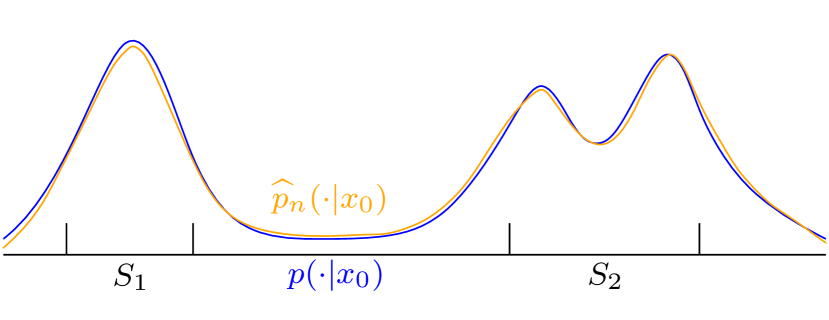
(a) True density $p(\,\cdot\,|\,x_{0})$ (blue) and the conditional density estimator $\widehat{p}_{n}(\,\cdot\,|\,x_{0})$ (yellow). High-density regions of $p(\,\cdot\,\,|\,x_{0})$ are marked by the intervals $S_{1}$ and $S_{2}$.

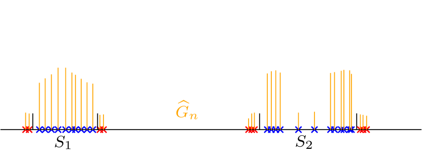
(b) Estimated (discrete) mixing measure $\widehat{G}_{n}$ after projecting $\widehat{p}_{n}(\,\cdot\,|\,x_{0})$. The $\times$s represent the atoms of $\widehat{G}_{n}$, the sticks represent the associated weights. Red $\times$s denote outliers.

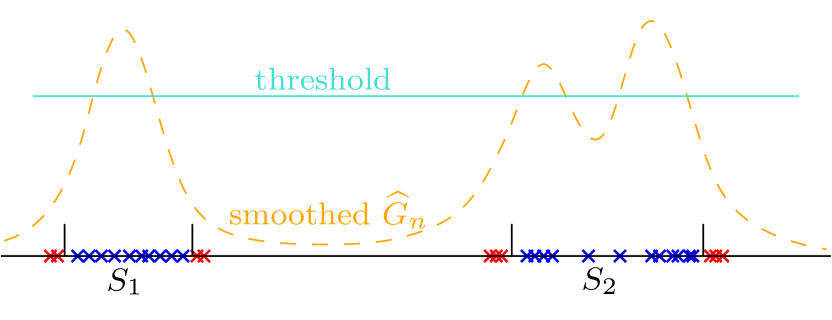
(c) Smoothed estimate of $\widehat{G}_{n}$ (note that this is different from $\widehat{p}_{n}(\,\cdot\,|\,x_{0})$) together with the estimated threshold used to locate high-density regions.

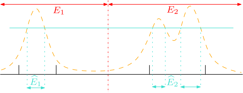
(d) Estimated high density regions $\widehat{E}_{1}$ and $\widehat{E}_{2}$, which are used to construct a partition $E_{1}\cup E_{2}$ of the real line.

Figure 2: Overview of the project-smooth-denoise procedure. The intervals $S_{1}$ and $S_{2}$ represent high-density regions of $p(\,\cdot\,\,|\,x_{0})$; see (15) for a formal definition. An (a) initial conditional density estimator $\widehat{p}_{n}(\,\cdot\,|\,x_{0})$ is (b) projected then (c) smoothed and denoised to construct a partition $(E_{1},E_{2})$ of the input space. The outputs are the estimated component mixing measures $\widehat{G}_{n}(\cdot\,|\,E_{1})$ and $\widehat{G}_{n}(\cdot\,|\,E_{2})$.

In order to present the main ideas at a high-level, here we give an overview of our proposed estimator. For fixed $x$, recall that the conditional density $p(\,\cdot\,\,|\,x)$ in (1) is itself a mixture model with $K$ components.

1. Construct a conditional density estimator $\widehat{p}_{n}(\,\cdot\,\,|\,x)$.

2. Estimate the mixing proportions and the error density using the following project-smooth-denoise procedure (Figure 2):

   1. Project $\widehat{p}_{n}(\,\cdot\,|\,x_{0})$ onto the space of mixture of Gaussians, where $x_{0}$ is a point of separation (Figure 2(b)).

   2. Smooth the obtained mixing measure $\widehat{G}_{n}$ to a density (Figure 2(c)).

   3. Denoise the original mixture by thresholding the smoothed density to recover the mixture components (Figure 2(d)).

3. Estimate the regression functions using a minimum distance estimator.

As mentioned, a crucial ingredient in the above procedure is the estimation of vanilla nonparametric mixtures (Step 2), whose discussion is separated into Section 5.

The rest of the paper is organized as follows. We review previous work in Section 2. In Section 3 we formalize our problem setup and assumptions, and state an identifiability result. Section 4 introduces an estimation procedure and shows its uniform consistency for certain families of mixed regression models. Section 5 discusses estimation of vanilla nonparametric mixtures, which is a key ingredient in estimating mixed regression models. Section 6 discusses several generalizations stemming from our model assumptions, and Section 7 concludes with some discussion. All proofs are deferred to the appendices; Appendix A contains detailed technical proofs, with additional supporting lemmas deferred to Appendices B and C.

Notation. For $1\leq p<\infty$ we shall denote $\|f\|_{L^{p}(S)}=(\int_{S}|f(x)|^{p}dx)^{1/p}$ and $\|f\|_{L^{\infty}(S)}=\operatorname{ess\,sup}_{x\in S}|f(x)|$ for a subset $S\subset\mathbb{R}$, and simply $\|f\|_{p}$ when $S=\mathbb{R}$. We denote $a\vee b=\operatorname{max}\{a,b\}$ and $a\wedge b=\operatorname{min}\{a,b\}$. The notation $\mathcal{F}$ stands for the Fourier transform and $\mathcal{F}^{-1}$ its inverse. For a density $\phi$ and a probability measure $G$, we denote $(\phi\ast G)(x)=\int\phi(x-\theta)dG(\theta)$ as their convolution. For two nonempty sets $A,B\subset\mathbb{R}$, we denote $\operatorname{dist}(A,B)=\operatorname{inf}_{x\in A,y\in B}|x-y|$. Lastly for two probability measures $P,Q$ over $\mathbb{R}$, the 1-Wasserstein distance is defined as

$$W_{1}(P,Q)=\underset{\gamma\in\Gamma(P,Q)}{\operatorname{inf}}\int_{\mathbb{R}\times\mathbb{R}}|x-y|d\gamma(x,y),$$ (3)

where $\gamma\in\Gamma(P,Q)$ denotes the set of all couplings between $P$ and $Q$.

2 Review of previous work

The prototypical mixture of regression model as in (1) would be one where both the $m_{k}$’s and $f$ are parametric, e.g., linear regression with Gaussian errors. Based on this, there have been many extensions that move beyond parametric regression functions, parametric errors, constant mixing proportions, or any combination of the three. In this section, we shall review some of the literature based on whether parametric assumptions are imposed on the regression functions. For our later developments, analysis of vanilla nonparametric mixtures turns out to be crucial, and we also give an updated account for them.

Parametric regression functions

Arguably the most popular version of the mixed regression (also known as mixture of regressions) model is the mixed linear regression model, which is the special case $m_{k}(X)=\langle\theta_{k},X\rangle$ in (1), where $\theta_{k}\in\mathbb{R}^{p}$. In this setting, Young and Hunter (2010); Huang and Yao (2012) extend the usual parametric model to allow covariate-dependent mixing proportions, and Hunter and Young (2012); Vandekerkhove (2013) study the case of general nonparametric errors. Focusing more on computational guarantees, Yi et al. (2014); Kwon and Caramanis (2020); Kwon et al. (2021) investigate convergence of EM algorithms and Chen et al. (2014); Hand and Joshi (2018); Li and Liang (2018); Yen et al. (2018) study estimation with low or optimal sample complexity, with Chen et al. (2014) also considering nonparametric errors. An excellent overview of mixed linear regression, and mixture models more broadly, is Frühwirth-Schnatter (2006).

Closely related to mixed linear regression models are so-called mixture of experts models (Jacobs et al., 1991; Jordan and Jacobs, 1994). In the mixture of experts model, it is assumed that (following the notation of Jiang and Tanner, 1999a)

$$p(y\,|\,x)=\sum_{j}g_{j}(x)\pi(h_{j}(x),y),$$ (4)

where $h_{j}(x)=\alpha_{j}+\langle\beta_{j},x\rangle$ is the linear mean response of $Y$ conditional on $X$. Related work on these models includes results on approximation (Jiang and Tanner, 1999a; Nguyen et al., 2016; Zeevi et al., 1998), identifiability (Jiang and Tanner, 1999b), and estimation (Makkuva et al., 2019; Ho et al., 2022b). There are two technical distinctions between mixtures of experts and mixtures of regressions: 1) The weights $g_{j}(x)$ (also known as the “gating functions”) are allowed to depend on $x$, and 2) The conditional mean functions $\pi(h_{j}(x),y)$ typically follow a very specific parametric (e.g. generalized linear) structure. At a more basic level, mixtures of experts are typically used to approximate a single, nonparametric response and are not in general identifiable. These distinctions stand in contrast to our setting in which the motivation is to identify and estimate the $K$ heterogeneous response curves $m_{k}(x)$.

Nonparametric regression functions

More closely related to our work are Huang et al. (2013); Xiang and Yao (2018), where the former considers a special case of (1) in which the error densities $f_{k}$ are Gaussian (i.e., $z_{k}\sim\mathcal{N}(0,\sigma_{k}^{2}(x))$) while allowing for general $\lambda_{k}(x)$, $m_{k}(x)$, and $\sigma_{k}^{2}(x)$. Here, the authors prove consistency and asymptotic normality for fixed $x$ by assuming the $m_{k}$ are differentiable and transversal, i.e., that the derivatives of each $m_{k}$ differ at points of intersection (see Figure 1). It is not hard to see why this condition is useful: If two regression functions are allowed to match derivatives at a point of intersection, then one can construct two smooth sets of regression functions that will yield the same joint $\mathbb{P}(X,Y)$: The original $m_{k}$ and $m_{j}$, as well as

$$\widetilde{m}_{k}(u)=\begin{cases}m_{k}(u)&u\leq x\\ m_{j}(u)&u\geq x\end{cases},\qquad\widetilde{m}_{j}(u)=\begin{cases}m_{j}(u)&u\leq x\\ m_{k}(u)&u\geq x\end{cases}.$$ (5)

Transversality implies that $\widetilde{m}_{k}$ and $\widetilde{m}_{j}$ as constructed above would be nondifferentiable at $x$, violating the differentiability requirement. A similar “non-parallel” condition appears in Kitamura and Laage (2018), where identifiability in nonparametric mixture models is studied in depth. Their approach to identifiability is based on moment generating functions, similar to Teicher (1963). Our approach is quite different to these works that stop short of proving uniform consistency, which is our main focus and more subtle than pointwise consistency. See Remark 6.3 for a more detailed comparison.

Another common approach to modeling heterogeneous regression functions is modal regression (Yao et al., 2012; Yao and Li, 2014; Chen et al., 2016), which aims to find the modes of the joint distribution $\mathbb{P}(X,Y)$. This is a flexible nonparametric model that provides an attractive alternative to parametric models for mixed regression, however, one notable drawback of modal regression is the inability to handle error distributions that are themselves multimodal, even if they are well-separated (see Figure 1). Modal regression also suffers from issues near points of intersection, as illustrated by Figure 2 in Chen et al. (2016).

Vanilla nonparametric mixtures

As indicated above, a key technical hurdle in the study of nonparametric mixed regression models is the identifiability of the conditional mixture for fixed $x$. As such, it is worth pausing to review what is known about identifiability in vanilla (i.e., covariate-free) nonparametric mixtures. For a detailed overview, see Frühwirth-Schnatter (2006) and Ritter (2014). By a nonparametric mixture, we mean a probability measure of the form $\mu=\sum_{k=1}^{K}\lambda_{k}\mu_{k}$, where $\mu_{k}$ are probability measures and $\lambda_{k}$ nonnegative weights summing to unity. It is clear that any probability measure $\mu$ can be written as a mixture in an infinite number of ways, simply by noting that $\mu(A)=\mu(A\,|\,E)\mu(E)+\mu(A\,|\,E^{c})\mu(E^{c})$ for any measurable sets $A$ and $E$. Clearly, additional assumptions are needed to ensure identifiability. For example, it is well-known that translation families and product mixtures are identifiable (Teicher, 1960, 1961, 1963, 1967), and a necessary and sufficient condition is linear independence of densities (Chandra, 1977; Yakowitz and Spragins, 1968). The use of minimum distance estimators to estimate the mixing measure is classical (Deely and Kruse, 1968), and there is a now refined analysis of optimality in estimating parametric mixtures (e.g. Ishwaran, 1996; Chen, 1995; Heinrich and Kahn, 2018; Ho and Nguyen, 2016, 2019). To the best of our knowledge, similar optimality results have not been obtained for nonparametric mixtures. Recent work focuses on nonparametric extensions when observations are grouped according to the latent class assignments (Vandermeulen and Scott, 2019; Ritchie et al., 2020), when the covariates carry certain latent structures (Allman et al., 2009; Gassiat and Rousseau, 2016), and when the component distributions are symmetric (Bordes et al., 2006; Hunter et al., 2007), products of univariate distributions (Hall and Zhou, 2003; Hall et al., 2005; Elmore et al., 2005), covariate-dependent (Compiani and Kitamura, 2016), or well-separated (Aragam et al., 2020). The basic thrust of this line of work on nonparametric identifiability is to restrict the component measures $\mu_{k}$ to satisfy various regularity assumptions such as independence, symmetry, or separation. In the present work, we build on the idea of separation studied in Aragam et al. (2020). Finally, we note that the models we introduce in the next section, based on convolutional mixtures, have appeared in a variety of contexts previously including Bayesian nonparametrics (Nguyen, 2013) and the empirical geometry of multivariate data (Koltchinskii, 2000).

3 Model assumptions and identifiability

We begin by presenting the details of our model assumptions and some preliminaries on identifiability in this section. We also briefly discuss pointwise vs. uniform consistency in these models.

3.1 Model assumptions

Recall the basic model (1). It follows that for any marginal density $p_{X}(x)$ over $x$, the joint density is specified as follows:

$$p(x,y)=p_{X}(x)\sum_{k=1}^{K}\lambda_{k}f(y-m_{k}(x)),\quad\quad(x,y)\in[a,b]\times\mathbb{R},$$ (6)

where $\sum_{k=1}^{K}\lambda_{k}=1$ and $f$ is a common error density satisfying $\int_{\mathbb{R}}xf(x)dx=0$. Throughout this paper, we shall assume $K$ is known and $\operatorname{min}_{k}\lambda_{k}>0$ so that (6) is indeed a $K$-component mixture model for each $x$; indeed when $K$ is unknown nonparametric mixtures are known to be fundamentally nonidentifiable, even under strong additional assumptions (see e.g. Aragam et al., 2020, Section 2.2). We also assume that $p_{X}>0$ on $[a,b]$ for simplicity; see Section 4.2.1 for discussion and Section 6.3 on how to generalize this. Consider the following parameter space

$$\mathcal{R}=\bigg{\{}\left(p_{X},f,\{\lambda_{k}\}_{k=1}^{K},\{m_{k}\}_{k=1}^{K}\right)\in\mathcal{P}([a,b])\times\mathcal{P}(\mathbb{R})\times\mathbb{R}^{K}\times[\mathcal{C}^{0}([a,b])]^{K}\mathrel{\mathop{\mathchar 58\relax}}$$

$$\underset{x\in[a,b]}{\operatorname{inf}}\,p_{X}(x)>0,\,\,\int_{\mathbb{R}}xf(x)dx=0,\,\,\underset{k=1,\ldots,K}{\operatorname{min}}\,\lambda_{k}>0,\,\,\sum_{k=1}^{K}\lambda_{k}=1\bigg{\}},$$

where $\mathcal{P}(\Omega)$ and $\mathcal{C}^{0}(\Omega)$ denote the set of all probability densities and the set of real-valued continuous functions on $\Omega\subset\mathbb{R}$, respectively. Let $\Phi\mathrel{\mathop{\mathchar 58\relax}}\mathcal{R}\rightarrow\mathcal{P}([a,b]\times\mathbb{R})$ be the map that associates a parameter tuple in $\mathcal{R}$ to the corresponding density (6). We say that a subfamily $\Phi(\mathcal{L})$ of $\Phi(\mathcal{R})$ with $\mathcal{L}\subset\mathcal{R}$ is identifiable if $\Phi$ is injective over $\mathcal{L}$. Without additional assumptions, the model $\Phi(\mathcal{R})$ is not identifiable, and therefore the purpose of this section is to introduce subfamilies of $\mathcal{R}$ over which identifiability is ensured.

Our main results are for the case where $f$ can be expressed as a Gaussian convolution as in (2). We do not assume that $G_{0}$ has a density. As we discuss in Section 5.1, even when they are identifiable, nonparametric mixtures may be poorly behaved, so this assumption is made in order to make uniform estimation feasible, although we do not believe it is fundamentally necessary and can likely be relaxed. The key structural assumption that we will exploit is the following idea of a point of separation.

Assumption 1 (Point of separation).

There exists $x_{0}\in[a,b]$ so that

$$\underset{j\neq k}{\operatorname{min}}\,|m_{j}(x_{0})-m_{k}(x_{0})|>2\operatorname{diam}(\operatorname{supp}(G_{0})).$$

In particular, we only require there be one such point of separation: Away from this point of separation, the $m_{k}$’s can be arbitrarily close and even intersect multiple times on the rest of the domain (see Figure 1). The rationale of this assumption is that if the regression functions stay close over the whole interval, then there is less hope to estimate each of them. Since the conditional density of (6) at $x_{0}$ is a convolutional Gaussian mixture with mixing measure $\sum_{k=1}^{K}\lambda_{k}G_{0}(\cdot-m_{k}(x_{0}))$, Assumption 1 is essentially requiring that the separation between the supports of $G_{0}(\cdot-m_{k}(x_{0}))$ is larger than their diameter so that single linkage clustering for instance can identify them. Under stronger assumptions on $G_{0}$, this assumption can be relaxed; see Section 5.4.

3.2 Identifiability

Before presenting our main results, we pause to discuss identifiability in the model $\Phi(\mathcal{R})$. See Kitamura and Laage (2018); Aragam et al. (2020) for a more detailed investigation of identifiability in nonparametric mixtures, including generalizations of some of the results below. Let $\mathcal{R}_{x_{0}}\subset\mathcal{R}$ be a subfamily satisfying the following conditions:

1. $f=\varphi_{\sigma}\ast G_{0}$ with $G_{0}$ having compact support (cf. (2)).

2. $\underset{j\neq k}{\operatorname{min}}\,|\lambda_{j}-\lambda_{k}|>0$.

3. $\underset{j\neq k}{\operatorname{min}}\,|m_{j}(x_{0})-m_{k}(x_{0})|>2\operatorname{diam}(\operatorname{supp}(G_{0}))$.

4. The set $Z=\{x\in[a,b]\mathrel{\mathop{\mathchar 58\relax}}\exists j\neq k,\,m_{j}(x)=m_{k}(x)\}$ is countable.

For obvious reasons, the value $x_{0}$ will be referred to as a point of separation and points in the set $Z$ will be referred to as points of intersection in the sequel.

Theorem 3.1.

The mixed regression model $\Phi(\mathcal{R}_{x_{0}})$ is identifiable.

Remark 3.2.

Apart from assuming a point of separation, we remark that another crucial assumption in the definition of $\mathcal{R}_{x_{0}}$ is that $\operatorname{min}_{j\neq k}|\lambda_{j}-\lambda_{k}|>0$, i.e., the mixing proportions are distinct. This will play an important role in the estimation procedure as we demonstrate in Section 4. Roughly speaking, the distinct mixing proportions can be used to solve the label switching issue near points where the regression functions intersect. Although we do not require that the $m_{k}$’s are differentiable for identifiability, Condition (A2) can be replaced by assuming the $m_{k}$’s are transversal (and hence differentiable) as in (Huang et al., 2013, Theorem 1). ∎

Remark 3.3.

The assumption (A2) rules out a set of weights that has measure zero and thus the model can be considered as generically identifiable (Allman et al., 2009) if we drop (A2). Similar conclusions have also been observed for parametric (Vandermeulen and Scott, 2019; Ho and Nguyen, 2019) and semiparametric (Hunter et al., 2007; Hunter and Young, 2012; Bordes et al., 2006) models. ∎

The proof of Theorem 3.1 can be found in Appendix A.2.1, but we illustrate the main idea here. First, we identify the error density and the mixing proportions by exploiting the point of separation $x_{0}$. By restricting the mixed regression model at $x_{0}$, the problem reduces to that of a finite mixture and we can make use of the following identifiability result of vanilla mixture models. Define

$$\mathscr{M}=\left\{\left(\{f_{k}\}_{k=1}^{K},\{\lambda_{k}\}_{k=1}^{K},\{\mu_{k}\}_{k=1}^{K}\right)\in\mathcal{P}(\mathbb{R})^{K}\times\mathbb{R}^{K}\times\mathbb{R}^{K}\right\}$$ (7)

to be the parameter space satisfying

1. $f_{k}=\varphi_{\sigma}\ast G_{k}$ with $G_{k}$ having compact support and $\int_{\mathbb{R}}xf_{k}(x)dx=0$.

2. $\underset{k}{\operatorname{min}}\,\lambda_{k}>0$ and $\sum_{k=1}^{K}\lambda_{k}=1$.

3. $\underset{j\neq k}{\operatorname{min}}\,\operatorname{dist}\left(\operatorname{supp}(G_{j}(\cdot-\mu_{j})),\,\operatorname{supp}(G_{k}(\cdot-\mu_{k}))\right)>\underset{k}{\operatorname{max}}\,\operatorname{diam}(\operatorname{supp}(G_{k}))$.

Here $G_{k}(\cdot-\mu_{k})$ is the translation of $G_{k}$ by $\mu_{k}$. Let $\Psi\mathrel{\mathop{\mathchar 58\relax}}\mathscr{M}\rightarrow\mathcal{P}(\mathbb{R})$ be the map that associates a parameter tuple $\big{(}\{f_{k}\}_{k=1}^{K},\{\lambda_{k}\}_{k=1}^{K},\{\mu_{k}\}_{k=1}^{K}\big{)}$ to the corresponding density $\sum_{k=1}^{K}\lambda_{k}f_{k}(\cdot-\mu_{k})$.

Proposition 3.4.

The mixture model $\Psi(\mathscr{M})$ is identifiable, i.e., $\Psi$ is injective over $\mathscr{M}$.

Remark 3.5.

Proposition 3.4 allows for different error densities for each component in the definition of $\mathscr{M}$ and can be seen as a special case of the general results from Aragam et al. (2020), although our proof is more straightforward owing to the additional structure provided by (B1). For mixed regression models, assumption (A3) implies that the conditional density $p(\,\cdot\,|\,x_{0})$ satisfies (B3) and so Proposition 3.4 gives identifiability of $f$ and $\{\lambda_{k}\}_{k=1}^{K}$. ∎

Once the error density and the mixing proportions have been identified, we see that the model (6) at each $x$ is then a finite mixture of the location family $\{f(\cdot-\mu)\}_{\mu\in\mathbb{R}}$, from which we can identify the values of the regression functions for each $x$. The difficulty would then to assemble the $m_{k}(x)$’s correctly across all $x\in[a,b]$. Since $Z$ is countable, we can decompose the interval $[a,b]$ as a union of subinterval $Z_{k}$’s where the $m_{k}$’s do not intersect. Continuity would allow us to correctly identify the $m_{k}$’s over each $Z_{k}$, however, a new difficulty arises when attempting to connect these $m_{k}$ across points of intersection (cf. (5)), as illustrated by the following example:

Example 1.

Consider a two-component mixed regression model

$$y|x\sim\begin{cases}m_{1}(x)+\varepsilon\quad\operatorname{w.p.}\,\,\lambda\\ m_{2}(x)+\varepsilon\quad\operatorname{w.p.}\,\,1-\lambda\end{cases}$$

where $m_{1}(x)=|x|,\,m_{2}(x)=-|x|$, $0<\lambda<1$ and $\varepsilon$ is Gaussian. Theorem 3.1 implies that the model is identifiable if $\lambda\neq\frac{1}{2}$. If $\lambda=\frac{1}{2}$, it is then indistinguishable from the alternate model with means $\tilde{m}_{1}(x)=-x$ and $\tilde{m}_{2}(x)=x$. The problem occurs precisely at the point $x=0$ when we try to connect the segments on either side. However if $\lambda\neq\frac{1}{2}$, then one can join the different pieces by matching the associated mixing proportions and there is a unique way to do so. In Huang et al. (2013), transversality was used to deal with this issue based on derivative information of the $m_{k}$’s. In particular, higher order smoothness assumptions can alleviate the label switching issue across points of intersection and guarantee identifiability. Nonetheless, we will show in Section 4.1 that even for $\mathcal{C}^{\infty}$ regression functions there are issues with uniformity if the mixing proportions are not distinct. ∎

In order to avoid this difficulty, Condition (A2) on distinct mixing proportions gives a unique way to assign the labels.

3.3 Pointwise vs. uniform consistency

Under the model assumptions introduced above, one can construct (pointwise) consistent estimators of the parameters $(f,\{\lambda_{k}\}_{k=1}^{K},$ $\{m_{k}\}_{k=1}^{K})$ by following the same steps as in the identifiability arguments. In other words, we can use the local information provided by the point of separation $x_{0}$ to construct estimators of the error density and the mixing proportions, which are then used to infer the regression functions globally. Let $\{(X_{i},Y_{i})\}_{i=1}^{n}$ be i.i.d. samples from the joint density (6).

Proposition 3.6.

Suppose $\mathcal{R}_{x_{0}}$ satisfies additionally

1. The joint density $p_{X}(x)\sum_{k=1}^{K}\lambda_{k}f(y-m_{k}(x))$ is $\beta$-Hölder continuous for some $\beta>0$.

Then there exists estimators $\widehat{f}_{n}$, $\{\widehat{\lambda}_{n,k}\}_{k=1}^{K}$ and $\{\widehat{m}_{n,k}\}_{k=1}^{K}$ so that with probability one

$$\|\widehat{f}_{n}-f\|_{1}\vee\underset{k}{\operatorname{max}}\,|\widehat{\lambda}_{n,k}-\lambda_{k}|\vee\underset{k}{\operatorname{max}}\,\|\widehat{m}_{n,k}-m_{k}\|_{L^{1}[a,b]}\xrightarrow{n\rightarrow\infty}0.$$

This result is a special case of more general results discussed in Section 6. Roughly speaking, consistent estimators $\widehat{f}_{n}$ and $\{\widehat{\lambda}_{n,k}\}_{k=1}^{K}$ can be obtained from a conditional density estimate $\widehat{p}_{n}(\,\cdot\,|\,x_{0})$ thanks to Assumption 1. A minimum distance estimator can then be employed to obtain the estimates $\{\widehat{m}_{n,k}(x)\}_{k=1}^{K}$ for each $x$, which are joined using (A2) to yield the $\widehat{m}_{n,k}$’s. This result extends to mixed regression models whose error densities are not necessarily convolutional Gaussian; see Section 6 for more discussion.

The crucial point here is that pointwise consistent estimators are relatively easy to obtain under our model assumptions, while uniformly consistent estimation requires substantially more efforts. As illustrated in Example 1, without additional regularity conditions on the $m_{k}$, it is impossible to decide how to “split” the curves past this intersection when the associated mixing proportions are equal (e.g., see the discussion around (5)). As we will show, without additional assumptions this issue about equal mixing proportions proves fatal when it comes to the existence of uniformly consistent estimators in this model (Section 4.1). Moreover, one might hope to extend the analysis of Huang et al. (2013) to nonparametric errors using recent work on nonparametric mixture models (Aragam et al., 2020), however, as we shall see these conditions also preclude uniformity in estimation (Section 5.1). Evidently, uniform consistency is a particularly subtle issue when it comes to nonparametric mixtures.

4 Uniformly consistent estimation of mixed regression

In this section we will study uniformly consistent estimation of the mixed regression model introduced in Section 3. As in Section 3.3, the high level idea is again similar to the identifiability argument but requires a more refined analysis to push through. As in the previous section, we assume that $f=\varphi_{\sigma}\ast G_{0}$ for some unknown $G_{0}$. To avoid technical digressions, we fix throughout the marginal density $p_{X}$, assuming $\operatorname{inf}_{[a,b]}\,p_{X}>0$ and $\|p_{X}\|_{L^{\infty}[a,b]}\vee\|p^{\prime}_{X}\|_{L^{\infty}[a,b]}<\infty$. Under these assumptions, let $\mathcal{U}_{x_{0}}\subset\mathcal{R}_{x_{0}}$ be a subfamily of tuples $\vartheta=(p_{X},f,\{\lambda_{k}\}_{k=1}^{K},\{m_{k}\}_{k=1}^{K})$ satisfying the following regularity assumptions:

1. $\underset{\vartheta\in\mathcal{U}_{x_{0}}}{\operatorname{sup}}\,\operatorname{diam}(\operatorname{supp}(G_{0}))<\infty$ and $\underset{\vartheta\in\mathcal{U}_{x_{0}}}{\operatorname{sup}}\,\Big{(}\underset{k}{\operatorname{max}}\,\|m_{k}\|_{L^{\infty}[a,b]}\vee\underset{k}{\operatorname{max}}\,\|m_{k}^{\prime}\|_{L^{\infty}[a,b]}\Big{)}<\infty$.

together with the following structural assumptions

1. $\underset{\vartheta\in\mathcal{U}_{x_{0}}}{\operatorname{inf}}\,\underset{j}{\operatorname{min}}\,\lambda_{j}>0,\quad\underset{\vartheta\in\mathcal{U}_{x_{0}}}{\operatorname{inf}}\,\underset{j\neq k}{\operatorname{min}}\,|\lambda_{j}-\lambda_{k}|>0.$

2. $\underset{\vartheta\in\mathcal{U}_{x_{0}}}{\operatorname{inf}}\,\Big{[}\underset{j\neq k}{\operatorname{min}}\,|m_{j}(x_{0})-m_{k}(x_{0})|-2\operatorname{diam}(\operatorname{supp}(G_{0}))\Big{]}>0.$

3. $\underset{\vartheta\in\mathcal{U}_{x_{0}}}{\operatorname{inf}}\,|(\mathcal{F}G_{0})(t)|\geq J(t)$ for some function $J>0$ and every $t$.

4. $\underset{\vartheta\in\mathcal{U}_{x_{0}}}{\operatorname{sup}}\,\operatorname{Leb}\!\big{(}\{x\mathrel{\mathop{\mathchar 58\relax}}\exists\,j\neq k,\,|m_{j}(x)-m_{k}(x)|\leq a_{n}\}\big{)}\xrightarrow{n\rightarrow\infty}0$ for all $a_{n}\rightarrow 0,$ where $\operatorname{Leb}(\cdot)$ denotes the Lebesgue measure of a set.

Additional discussion on these assumptions can be found in Remark 4.2. The main result in this section is the following:

Theorem 4.1.

There exist uniformly consistent estimators $\widehat{f}_{n}$, $\{\widehat{\lambda}_{n,k}\}_{k=1}^{K}$, and $\{\widehat{m}_{n,k}\}_{k=1}^{K}$ for $\mathcal{U}_{x_{0}}$, where is $\mathcal{U}_{x_{0}}$ is defined by (C1)-(C5). More specifically, for any $\varepsilon>0$,

$$\underset{\mathcal{U}_{x_{0}}}{\operatorname{sup}}\,\,\mathbb{P}\left(\|\widehat{f}_{n}-f\|_{1}\vee\underset{k}{\operatorname{max}}\,|\widehat{\lambda}_{n,k}-\lambda_{k}|\vee\underset{k}{\operatorname{max}}\,\|\widehat{m}_{n,k}-m_{k}\|_{L^{1}[a,b]}>\varepsilon\right)\xrightarrow{n\rightarrow\infty}0.$$

The remainder of this section is devoted to discussing this result and its assumptions in detail, along with a proof outline that constructs the estimators explicitly. More specifically, in Section 4.2, we outline the main ideas behind the constructive proof of Theorem 4.1, while deferring technical details to Appendix A.3.

We emphasize that these estimators are not abstract, and will be explicitly constructed in the sequel. There are three main steps:

1. Estimation of the conditional density $p(\cdot\,|\,x)$ via kernel density estimators (Section 4.2.1);

2. Estimation of $\lambda_{k}$ and $f$ via estimation of the vanilla mixture model $p(\cdot\,|\,x_{0})$ (Section 4.2.2; details in Section 5);

3. Estimation of the regression functions $m_{k}$ via a minimum distance estimator (Section 4.2.3).

Throughout, we assume that $x_{0}$ and $\sigma$ are known, which is crucial to illustrating our main point that uniform consistency is challenging even under such knowledge—i.e. the difficulties are not somehow due to orthogonal problems in estimating the variance or points of separation. The second step above is the most delicate, and involves a careful project-smooth-denoise construction that is detailed in Section 5.

Remark 4.2.

We now discuss briefly the assumptions made on $\mathcal{U}_{x_{0}}$.

• (C1)-(C3) are simply uniform versions of those in (A1)-(A3).

• (C1) ensures a uniformly consistent conditional density estimator as a crucial first step. To focus on mixture models, we assume the $m_{k}$ are differentiable in (C1) for simplicity, however, we expect that a similar result assuming only weaker Hölder-type continuity is possible. We remark that it is only in this step that we need the differentiability of $p_{X}$ and the $m_{k}$’s.

• (C2) is of utmost importance: We show below by example that uniform consistency is impossible without assuming distinct mixing proportions (see also Remark 3.2).

• (C3) is a crucial separation condition that allows different mixture components to be identified as in Section 3.2 and will be the key structural assumption that we exploit for estimating vanilla nonparametric mixtures in Section 5. This can be relaxed under strong regularity assumptions on $G_{0}$ that we discuss in Section 5.4.

• (C4) is a technical assumption to ensure a modulus-of-continuity type result (11) for finite mixture models and allows a wide range of nonparametric $G_{0}$’s as discussed in Section 4.3.1. This type of assumption is standard in the nonparametric deconvolution literature (Fan, 1991; Nguyen, 2013), where $J$ is usually taken to be $c|t|^{-\beta}$ or $c\exp(-|t|^{\beta}/\gamma)$ for constants $c,\beta,\gamma$.

• (C5) controls the separation between different regression functions around points of intersection and will be discussed in more detail in Section 4.3.2. In particular, this assumption is satisfied under a uniform version of the transversality assumption from Huang et al. (2013). We also provide an example where transversality fails (Example 5), thereby proving that this is not necessary. ∎

4.1 Nonexistence of uniformly consistent estimators

Before describing the estimator, we illustrate why the second part of Condition (C2) is crucial, which might be somewhat surprising at first. Consider the mixed regression model

$$(\mathscr{P})\mathrel{\mathop{\mathchar 58\relax}}\quad y|x\sim\begin{cases}m_{1}(x)+\varepsilon\quad\operatorname{w.p.}\,\,\frac{1}{2}\\ m_{2}(x)+\varepsilon\quad\operatorname{w.p.}\,\,\frac{1}{2}\end{cases}$$

where $m_{1},m_{2}\in\mathcal{C}^{\infty}(\mathbb{R})$ and $\varepsilon$ is Gaussian. Let $\{(X_{i},Y_{i})\}_{i=1}^{n}$ be i.i.d. samples from it. We will construct an alternate model that generates the same data distribution as $\mathscr{P}$. Without loss of generality assume there are no $X_{i}$’s that lie in between $u\mathrel{\mathop{\mathchar 58\relax}}=X_{1}$ and $v\mathrel{\mathop{\mathchar 58\relax}}=X_{2}$ and that $u<v$. Let $\varphi\in\mathcal{C}^{\infty}(\mathbb{R})$ be a smooth function satisfying $\varphi=0$ for $x\leq u$ and $\varphi=1$ for $x\geq v$, and define

$$\widetilde{m}_{1} =(1-\varphi)m_{1}+\varphi m_{2}$$

$$\widetilde{m}_{2} =(1-\varphi)m_{2}+\varphi m_{1}.$$

We then have $\widetilde{m}_{1},\widetilde{m}_{2}\in\mathcal{C}^{\infty}(\mathbb{R})$ and

$$\widetilde{m}_{1}=\begin{cases}m_{1}\quad&x\leq u\\ m_{2}\quad&x\geq v\end{cases}\quad\quad\widetilde{m}_{2}=\begin{cases}m_{2}\quad&x\leq u\\ m_{1}\quad&x\geq v\end{cases}.$$

In particular the two models

$$(\mathscr{P})\mathrel{\mathop{\mathchar 58\relax}}\quad y|x\sim\begin{cases}m_{1}(x)+\varepsilon\quad\operatorname{w.p.}\,\,\frac{1}{2}\\ m_{2}(x)+\varepsilon\quad\operatorname{w.p.}\,\,\frac{1}{2}\end{cases}\quad(\mathscr{P}_{n})\mathrel{\mathop{\mathchar 58\relax}}\quad y|x\sim\begin{cases}\widetilde{m}_{1}(x)+\varepsilon\quad\operatorname{w.p.}\,\,\frac{1}{2}\\ \widetilde{m}_{2}(x)+\varepsilon\quad\operatorname{w.p.}\,\,\frac{1}{2}\end{cases}$$

have the same conditional distribution on $(-\infty,u]\cup[v,\infty)$ and any estimator based on $\{(X_{i},Y_{i})\}_{i=1}^{n}$ cannot distinguish between them. Notice that the construction of such a $\mathscr{P}_{n}$ can be carried out for every $n$, giving a sequence of models $\{\mathscr{P}\}_{n=2}^{\infty}$, each of which is indistinguishable from $\mathscr{P}$ based on data $\{(X_{i},Y_{i})\}_{i=1}^{n}$. Hence there cannot be a uniformly consistent estimator for the regression functions over subfamilies of $\mathcal{R}_{x_{0}}$ that allow equal mixing proportions even if the $m_{k}$’s are restricted to be $\mathcal{C}^{\infty}(\mathbb{R}).$ The problem lies precisely in the fact that in between any two adjacent $X_{i}$’s, the model could undergo a label switching and no degree of smoothness can prevent this if the mixing proportions are equal. In particular, the best one can do in this case is to estimate the function values $m_{k}(x)$ for fixed $x$ but not how to connect them. Similar problems arise in mixtures with more than two components, where one is not expected to estimate those components with equal mixing proportions.

4.2 Construction of estimator

Throughout this section we assume to be given $n$ i.i.d. samples $\{(X_{i},Y_{i})\}_{i=1}^{n}$ from the model (6). The estimation procedure starts by constructing a conditional density estimator $\widehat{p}_{n}(y|x)$ of the mixed regression model (Section 4.2.1). By exploiting the point of separation $x_{0}$ in Assumption 1, we will then construct estimators of the error density and the mixing proportions (Section 4.2.2) based on $\widehat{p}_{n}(\,\cdot\,|\,x_{0})$. The remaining estimation of the regression functions for a fixed $x$ reduces to a parametric estimation problem, where a minimum distance estimator is employed to achieve $L^{1}$ (as opposed to pointwise) approximation (Section 4.2.3). While introducing in detail each of these steps, we shall see how the assumptions (C1)-(C5) progressively build up.

4.2.1 Conditional density estimator

Our estimation procedure starts by estimating the conditional density. Conditional density estimators have been studied extensively in the literature (e.g. De Gooijer and Zerom, 2003; Efromovich, 2007, 2005; Li et al., 2022), but a precise $L^{1}$ rate result (with explicit dependence on all the model parameters) seems to be missing. Therefore, to make our presentation self-contained, we include such a construction and bound its $L^{1}$ error in Appendix C.1. As noted in Remark 4.2, this step is the only step in which differentiability of the regression functions is needed, and we further assume $p_{X}$ is bounded away from zero so that a simple ratio of kernel density estimators (KDE) will suffice in our setting, although more sophisticated estimators exist under weaker assumptions. More precisely, let $\widehat{p}_{n}(x,y)$ be a KDE for the joint density $p(x,y)$ and $\widehat{p}_{X,n}(x)$ be a KDE for the marginal density $p_{X}(x)$. We have the following result:

Proposition 4.3.

Let $\widehat{p}_{n}(\,\cdot\,|\,x)=\widehat{p}_{n}(x,\cdot)/\widehat{p}_{X,n}(x)$ be a ratio of kernel density estimators with the box kernel $H=\frac{1}{2}\mathbf{1}_{[-1,1]}$, with bandwidth $h_{n}$ satisfying

$$h_{n}\rightarrow 0,\quad\frac{nh_{n}^{2}}{|\log h_{n}|}\rightarrow\infty,\quad\frac{|\log h_{n}|}{\log\log n}\rightarrow\infty,\quad h_{n}^{2}\leq ch_{2n}^{2}$$

for some $c>0$. Let $\mathcal{V}_{x_{0}}\subset\mathcal{R}_{x_{0}}$ be a subfamily satisfying (C1). Then we have

$$\underset{\mathcal{V}_{x_{0}}}{\operatorname{sup}}\,\underset{x\in[a+h_{n},b-h_{n}]}{\operatorname{sup}}\,\mathbb{E}\|\widehat{p}_{n}(\,\cdot\,|\,x)-p(\,\cdot\,|\,x)\|_{1} \xrightarrow{n\rightarrow\infty}0.$$ (8)

Remark 4.4.

In the sequel, any conditional density estimator satisfying (8) suffices. Possible choices of the bandwidth include $h_{n}\asymp n^{-1/(2+\beta)}$ for any $\beta>0$. ∎

4.2.2 Estimating the error density and mixing proportions

The next step is to construct estimators of the error density $f$ and the mixing proportions $\lambda_{k}$. Similarly as the discussion before Proposition 3.4, the problem in this subsection reduces to that of a finite mixture and can be decoupled from the other parts. Since these results may be of independent interest, we defer the details to Section 5, where a complete description of the estimator and its analysis can be found.

The estimator is based on a novel “project-smooth-denoise” construction. The rough idea is to first project $\widehat{p}_{n}(\,\cdot\,|\,x_{0})$ onto finite mixtures of Gaussians to get an approximation of the mixing measure $\sum_{k=1}^{K}\lambda_{k}G_{0}(\cdot-m_{k}(x_{0}))$ and then employ a careful smooth-denoise step to recover the individual components $(\lambda_{k},G_{0}(\cdot-m_{k}(x_{0})))$, from which we obtain the estimates $\widehat{f}_{n}$ and $\{\widehat{\lambda}_{n,k}\}_{k=1}^{K}$ (cf. Figure 2). This is where the point of separation $x_{0}$ is used: By (1), $p(\,\cdot\,|\,x_{0})$ can be interpreted as a finite mixture, and the separation enables estimation of this mixture (see discussion surrounding Assumption 1). The following result, as a corollary of Theorem 5.1 applied to $p(\,\cdot\,|\,x_{0})$, establishes that this procedure provides uniformly consistent estimation of the mixture model at $x_{0}$.

Proposition 4.5.

Let $\mathcal{V}_{x_{0}}\subset\mathcal{R}_{x_{0}}$ be a subfamily satisfying (C1)-(C3). There exist estimators $\widehat{f}_{n}$, $\{\widehat{\lambda}_{n,k}\}_{k=1}^{K}$, and a sequence $\varepsilon_{n}\rightarrow 0$ so that

$$\underset{\mathcal{V}_{x_{0}}}{\operatorname{sup}}\,\,\mathbb{P}\left(\|\widehat{f}_{n}-f\|_{1}\vee\underset{k}{\operatorname{max}}\,|\widehat{\lambda}_{n,k}-\lambda_{k}|>\varepsilon_{n}\right)\xrightarrow{n\rightarrow\infty}0.$$

Remark 4.6.

A direct application of Theorem 5.1 implies consistency up to a permutation. Since now the mixing proportions are uniformly separated, so are the estimates $\widehat{\lambda}_{n,k}$’s asymptotically. Hence after a relabelling which sorts both $\{\widehat{\lambda}_{n,k}\}_{k=1}^{K}$ and $\{\lambda_{k}\}_{k=1}^{K}$ in increasing order, the permutation will be the identity uniformly over $\mathcal{V}_{x_{0}}$ for all large $n$. This additional step is not necessary but is adopted for notational convenience. ∎

4.2.3 Estimating the regression functions

Now it remains to introduce estimators for the regression functions $m_{k}$ via the following minimum distance estimator: Let $B$ be a constant so that $\operatorname{max}_{k}\|m_{k}\|_{L^{\infty}[a,b]}\leq B$ (this could be chosen based on assumption (C1) or to be sufficiently large based on data). Define for $x\in[a,b]$

$$(\widehat{m}_{n,1}(x),\ldots,\widehat{m}_{n,K}(x))^{T}=\underset{\theta\in[-B,B]^{K}}{\operatorname{arg\,min}}\,\left\|\sum_{k=1}^{K}\widehat{\lambda}_{n,k}\widehat{f}_{n}(\cdot-\theta_{k})-\widehat{p}_{n}(\,\cdot\,|\,x)\right\|_{1},$$ (9)

where we take any minimizer if there are multiple ones.

Lemma 4.7.

Suppose $\operatorname{min}_{k}\lambda_{k}>0$ and $|\mathcal{F}G_{0}|\geq J$ for some function $J>0$. For each fixed $x\in[a,b]$ we have

$$\underset{k}{\operatorname{max}}\,\,\underset{j}{\operatorname{min}}\,|\widehat{m}_{n,j}(x)-m_{k}(x)|\leq\frac{e_{n}(x)}{\operatorname{min}_{k}\lambda_{k}},$$

where

$$e_{n}(x)=C_{B}F_{J,\sigma}\Big{(}\|\widehat{f}_{n}-f\|_{1}+\sum_{k=1}^{K}|\widehat{\lambda}_{n,k}-\lambda_{k}|+\|\widehat{p}_{n}(\,\cdot\,|\,x)-p(\,\cdot\,|\,x)\|_{1}\Big{)}$$

with $C_{B}$ a constant depending only on $B$ and $F_{J,\sigma}$ a strictly increasing function depending only on $J,\sigma$ that satisfies $F_{J,\sigma}(d)\xrightarrow{d\rightarrow 0}0$. Furthermore if $\operatorname{min}_{j\neq k}|\lambda_{j}-\lambda_{k}|>0$ and

$$\underset{j\neq k}{\operatorname{min}}\,|m_{j}(x)-m_{k}(x)|>\frac{6e_{n}(x)}{\operatorname{min}_{k}\lambda_{k}\wedge\operatorname{min}_{j\neq k}|\lambda_{j}-\lambda_{k}|}$$ (10)

then

$$\underset{k}{\operatorname{max}}\,|\widehat{m}_{n,k}(x)-m_{k}(x)|\leq\frac{e_{n}(x)}{\operatorname{min}_{k}\lambda_{k}}.$$

The key in proving Lemma 4.7 is the following modulus-of-continuity type result (Lemma B.2) that slightly generalizes (Nguyen, 2013, Theorem 2):

$$W_{1}(\widehat{V},V)\leq C_{B}F_{J,\sigma}\big{(}\|\widehat{V}\ast f-V\ast f\|_{1}\big{)},\quad\widehat{V}=\sum_{k=1}^{K}\lambda_{k}\delta_{\widehat{m}_{n,k}(x)},\quad V=\sum_{k=1}^{K}\lambda_{k}\delta_{m_{k}(x)}.$$ (11)

Here, $W_{1}$ is the 1-Wasserstein distance defined as in (3) and $\delta_{a}$ is the Dirac delta at a point $a\in\mathbb{R}$.

For each mixed regression model the lower bound function $J$ can be taken as $|\mathcal{F}G_{0}|$ provided that it never vanishes, but a uniform lower bound as in (C4) is needed for uniform consistency. In Section 4.3.1 we explicitly construct families of compactly supported $G_{0}$’s satisfying (C4).

Lemma 4.7 establishes error estimates over regions where the $m_{k}$’s satisfy (10). Since the error $e_{n}(x)\rightarrow 0$ in probability over $[a+h_{n},b-h_{n}]$ (by Propositions 4.3 and 4.5), such regions will eventually be the whole interval $(a,b)$ so that we can achieve consistent estimation in $L^{1}[a,b]$ norm. Before stating the result, however, we make a further remark on how the assumption of distinct mixing proportions enters our estimation procedure (9). In particular, we have defined the function estimate $\widehat{m}_{n,k}$ to be the collection of all $\widehat{m}_{n,k}(x)$’s that are associated with $\widehat{\lambda}_{n,k}$. Since the $\lambda_{k}$’s are distinct, so are the estimates $\widehat{\lambda}_{n,k}$’s asymptotically and hence this defines a unique consistent labelling procedure for the estimates $\{\widehat{m}_{n,k}(x)\}_{k=1}^{K}$.

By combining these observations, we can prove $L^{1}$ consistency of the resulting regression estimates:

Proposition 4.8.

Let $\mathcal{V}_{x_{0}}\subset\mathcal{R}_{x_{0}}$ be a subfamily satisfying (C1)-(C5). Then the estimators $\{\widehat{m}_{n,k}\}_{k=1}^{K}$ are uniformly consistent, i.e., for any $\varepsilon>0$

$$\underset{\mathcal{V}_{x_{0}}}{\operatorname{sup}}\,\,\mathbb{P}\Big{(}\underset{k}{\operatorname{max}}\,\|\widehat{m}_{n,k}-m_{k}\|_{L^{1}[a,b]}>\varepsilon\Big{)}\xrightarrow{n\rightarrow\infty}0.$$

It is in this step (i.e., extending estimates for fixed $x$ to $L^{1}$ consistency) that (C5) is invoked. It can be understood as a uniform control on the regions where (10) is not satisfied, i.e., regions where the pointwise estimates are not provably accurate.

4.3 Discussion of conditions

Most of the conditions in (C1)-(C5) are easily interpreted, however, (C4)-(C5) are more technical and perhaps a bit opaque. We pause here to discuss these conditions in more detail.

4.3.1 Discussion of Condition (C4)

The following example provides nonparametric families of functions that satisfy (C4). Recall $G_{0}$ as defined in (2).

Example 2.

Let $\ell>0$ be a function. Consider the collection of mixing measures $dG_{0}=gdx$ with $g$ belonging to

$$\mathcal{G}_{\ell}=\left\{g=\frac{(\phi\ast\phi)\cdot q}{\int_{\mathbb{R}}(\phi\ast\phi)\cdot q\,dx}\mathrel{\mathop{\mathchar 58\relax}}\phi=\frac{1}{2}\mathbf{1}_{[-1,1]},q\text{ is a density such that }\mathcal{F}q\geq\ell\right\}.$$

Possible examples of the function $\ell$ are $c\exp(-|t|^{\beta}/\gamma)$ and $c|t|^{-\beta}$ for some constants $c,\beta,\gamma$, which characterize distributions that are supersmooth and smooth of order $\beta$ respectively (Fan, 1991; Nguyen, 2013). Notice that without the constraint of having a compact support, the set of such $q$’s already satisfies (C4). The additional term $\phi\ast\phi$ can be interpreted as a truncation to make $q$ compactly supported. We see that the family $\mathcal{G}_{\ell}$ satisfies $\operatorname{inf}_{g\in\mathcal{G}_{\ell}}|\mathcal{F}g|\geq J$ for some function $J>0$. Indeed, notice that

$$\int_{\mathbb{R}}\phi\ast\phi\cdot q\,dx\leq\|\phi\ast\phi\|_{\infty}$$

since $q$ is a density, so that

$$|\mathcal{F}g(w)|\geq\frac{1}{\|\phi\ast\phi\|_{\infty}}\left|\big{(}(\mathcal{F}q)\ast(\mathcal{F}\phi)^{2}\big{)}(w)\right|\geq\frac{1}{\|\phi\ast\phi\|_{\infty}}\int_{\mathbb{R}}\ell(w-t)\frac{\sin^{2}(t)}{t^{2}}dt=\mathrel{\mathop{\mathchar 58\relax}}J>0.$$

We remark that $\phi\ast\phi$ can be replaced with any bounded nonnegative compactly supported function whose Fourier transform is also nonnegative. ∎

Example 3.

We can modify Example 2 as follows to drop the assumption that $q$ is a density. Let $0<\ell\leq u\in L^{2}(\mathbb{R})$ be two functions. Consider the collection of mixing measures $dG_{0}=g\,dx$ with $g$ belonging to

$$\mathcal{G}_{\ell,u}=\left\{g=\frac{(\phi\ast\phi)\cdot q}{\int_{\mathbb{R}}(\phi\ast\phi)\cdot q\,dx}\mathrel{\mathop{\mathchar 58\relax}}\phi=\frac{1}{2}\mathbf{1}_{[-1,1]},\,\,q=|\mathcal{F}^{-1}v|^{2}\,\,\operatorname{with}\,\,\ell\leq v\leq u\right\},$$

where $|\cdot|$ denotes the modulus of a possibly complex number. Similarly as in Example 2, it suffices to show that $\mathcal{F}q$ is uniformly lower bounded by a positive function and that the denominator uniformly upper bounded. This follows by noticing that $q(x)=(\mathcal{F}^{-1}v)(x)(\mathcal{F}^{-1}v)(-x)$ since $v$ is real, and

$$(\mathcal{F}q)(w)=\int_{\mathbb{R}}v(w-t)v(-t)dt\geq\int_{\mathbb{R}}\ell(w-t)\ell(-t)dt>0.$$

Moreover, we have

$$\int_{\mathbb{R}}(\phi\ast\phi)\cdot q\,dx\leq\|\phi\ast\phi\|_{\infty}\int_{\mathbb{R}}q\,dx \leq\|\phi\ast\phi\|_{\infty}\int_{\mathbb{R}}|\mathcal{F}^{-1}v|^{2}dx$$

$$=\|\phi\ast\phi\|_{\infty}\int_{\mathbb{R}}v^{2}dx\leq\|\phi\ast\phi\|_{\infty}\|u\|_{2}^{2}.$$

∎

4.3.2 Discussion of Condition (C5)

Roughly speaking, Condition (C5) prevents different regression functions from becoming arbitrarily close over an entire interval. For a single model where the $m_{k}$’s only intersect at countably many points, we have

$$\left\{x\mathrel{\mathop{\mathchar 58\relax}}\exists\,j\neq k,\,|m_{j}(x)-m_{k}(x)|\leq a_{n}\right\}\searrow\left\{x\mathrel{\mathop{\mathchar 58\relax}}\exists\,j\neq k,\,m_{j}(x)=m_{k}(x)\right\},$$

which has measure zero and therefore (C5) can be seen as a uniform analog of this fact. The reason why we need such assumption has been foreshadowed in Lemma 4.7 above in that we need uniform control on the size of the set where (10) fails.

To better understand Condition (C5), let us further introduce sufficient conditions on the $m_{k}$’s that guarantee it. The first observation is that (C5) is satisfied if the $m_{k}$’s are uniformly separated, however, this excludes intersections of the $m_{k}$’s and is less interesting. The following example generalizes this to allow intersections.

Example 4.

For $j\neq k$, let $Z_{jk}=\{x\mathrel{\mathop{\mathchar 58\relax}}m_{j}(x)=m_{k}(x)\}$ and $Z_{jk}(\delta)=\{x\mathrel{\mathop{\mathchar 58\relax}}\operatorname{dist}(x,Z_{jk})<\delta\}$. Suppose there exists $N\in\mathbb{N},\delta,\eta>0$ so that for all $\vartheta\in\mathcal{U}_{x_{0}}$

$$\underset{j\neq k}{\operatorname{max}}\,\operatorname{Card}(Z_{jk})\leq N,\qquad\underset{j\neq k}{\operatorname{min}}\,\underset{x\in Z_{jk}(\delta)^{c}}{\operatorname{inf}}\,|m_{j}(x)-m_{k}(x)|\geq\eta,$$ (12)

$$\qquad\qquad\qquad\underset{j\neq k}{\operatorname{min}}\,\underset{x\in Z_{jk}(\delta)}{\operatorname{inf}}\,|m^{\prime}_{j}(x)-m^{\prime}_{k}(x)|\geq\eta.$$

Lemma B.3 shows that (12) implies (C5). These conditions essentially require uniform separation of the $m_{k}$’s away from the points of intersection and uniform separation of the derivatives $m_{k}^{\prime}$’s near points of intersection. The latter will guarantee that two regression functions do not stay close over a large interval when they intersect. ∎

The conditions in (12) can be interpreted as a uniform version of transversality introduced in Huang et al. (2013). We remark that although sufficient, uniform transversality is not necessary for (C5) to be satisfied as illustrated by the following example.

Example 5.

Consider the family of pairs of functions $\mathscr{R}_{P,C}=\{(0,cx^{p})\mathrel{\mathop{\mathchar 58\relax}}x\in[0,1],0\leq p\leq P,\,c\geq C\}$ for some fixed $P,C>0$. First, observe that for any $P\geq 1,C>0$, $\mathscr{R}_{P,C}$ violates the transversality condition and (12). Next, if $P\to\infty$ or $C\to 0$, then there are nonzero functions in $\mathscr{R}_{P,C}$ that approximate the zero function uniformly over small intervals around the origin, ostensibly in violation of (C5), but for fixed $P,C>0$ this issue is avoided. More precisely, for any $a_{n}\rightarrow 0$ we have when $a_{n}\leq C$

$$\underset{\mathscr{R}_{P,C}}{\operatorname{sup}}\,\operatorname{Leb}\left(\{|m_{1}-m_{2}|\leq a_{n}\}\right)\leq\left(\frac{a_{n}}{C}\right)^{1/P}\xrightarrow{n\rightarrow\infty}0.$$

Therefore the family of two-component mixed regression models with regression functions in $\mathscr{R}_{P,C}$ satisfies (C5). This example illustrates a typical situation where the separation around a point of intersection is controlled by the condition $c\geq C$. ∎

4.4 A concrete family

We close this section by demonstrating Theorem 4.1 through a concrete example under which all of the assumptions hold. As our original goal was to present a (nearly) minimal set of conditions under which uniform consistency is assured, the resulting Conditions (C1)-(C5) are somewhat abstract (see also Remark 4.2). Using the examples in Section 4.3, however, we can now present a more concrete set of assumptions, albeit at the expense of some generality.

Consider the following family of two-component mixed regression models over the interval $[a,b]$. The assumption that $K=2$ is only for simplicity, and this example can easily be generalized to $K>2$. Define

$$\mathcal{V}=\big{\{}(p_{X},f,\{\lambda_{k}\}_{k=1}^{2},\{m_{k}\}_{k=1}^{2})\big{\}}$$

as the set of tuples such that for some $x_{0}\in[a,b]$, some $N\in\mathbb{N}$, and some small $\epsilon_{1},\epsilon_{2},\xi,\delta,\eta>0$, the following conditions hold:

1. $p_{X}=\operatorname{Unif}[a,b]$.

2. $\lambda_{1}\wedge\lambda_{2}\geq\epsilon_{1}$ and $|\lambda_{1}-\lambda_{2}|\geq\epsilon_{2}$.

3. $|m_{1}(x_{0})-m_{2}(x_{0})|-2\operatorname{diam}(\operatorname{supp}(G_{0}))\geq\xi.$

4. $f=\varphi_{\sigma}\ast G_{0}$ with $G_{0}$ as in Example 2.

5. The set $Z$ of points of intersection between $m_{1}$ and $m_{2}$ has at most $N$ elements, with

   $$\underset{x\in Z(\delta)^{c}}{\operatorname{inf}}|m_{1}(x)-m_{2}(x)|\geq\eta,\quad\underset{x\in Z(\delta)}{\operatorname{inf}}|m_{1}^{\prime}(x)-m_{2}^{\prime}(x)|\geq\eta,$$

   where $Z(\delta)=\{x\mathrel{\mathop{\mathchar 58\relax}}\operatorname{dist}(x,Z)\leq\delta\}$.

Under these conditions, Theorem 4.1 applies to the family $\mathcal{V}$:

Corollary 4.9.

There exist uniformly consistent estimators for $(f,\{\lambda_{k}\}_{k=1}^{2},\{m_{k}\}_{k=1}^{2})$ over $\mathcal{V}$.

We remark that this only serves as one such concrete example: Additional ones can be constructed by combining Examples 2-5 in different ways.

5 Uniformly consistent estimation of mixture models

In this section we consider estimation of vanilla nonparametric mixtures as in (7), thereby completing the missing piece from Section 4.2.2. As mentioned, the estimation procedure to be introduced applies to finite mixture models and we shall restrict ourselves to the family $\mathscr{M}$ defined by (7). In particular, unlike the previous section, we now allow the mixture components $f_{k}$ to be distinct, and treat the case $f_{k}\equiv f$ (i.e., as in the previous section) for all $k$ as a special case. Recall that $f_{k}=\varphi_{\sigma}\ast G_{k}$ with $G_{k}$ having compact support.

The main result in this section is the following. Let $\mathscr{U}\subset\mathscr{M}$ be a subfamily of tuples $\vartheta=(\{f_{k}\}_{k=1}^{K},\{\lambda_{k}\}_{k=1}^{K},\{\mu_{k}\}_{k=1}^{K})$ satisfying

1. $\underset{\vartheta\in\mathscr{U}}{\operatorname{sup}}\,\underset{k}{\operatorname{max}}\,\big{[}\operatorname{diam}(\operatorname{supp}(G_{k}))\vee\mu_{k}\big{]}<\infty$.

2. $\underset{\vartheta\in\mathscr{U}}{\operatorname{inf}}\,\underset{k}{\operatorname{min}}\,\lambda_{k}>0$.

3. $\underset{\vartheta\in\mathscr{U}}{\operatorname{inf}}\,\Big{[}\underset{j\neq k}{\operatorname{min}}\,\operatorname{dist}\left(\operatorname{supp}(G_{j}(\cdot-\mu_{j})),\,\operatorname{supp}(G_{k}(\cdot-\mu_{k}))\right)-\underset{k}{\operatorname{max}}\,\operatorname{diam}(\operatorname{supp}(G_{k}))\Big{]}>0$.

We have the following result:

Theorem 5.1.

There exist uniformly consistent estimators $\widehat{\lambda}_{n,k}$ and $\widehat{f}_{n,k}$ for $\mathscr{U}$, where $\mathscr{U}$ is defined by (D1)-(D3). More specifically, there exists a permutation $\Pi=\Pi(\vartheta,n)$ and a sequence $\varepsilon_{n}\rightarrow 0$ such that

$$\underset{\mathscr{U}}{\operatorname{sup}}\,\,\mathbb{P}\Big{(}\underset{k}{\operatorname{max}}\,\left(|\widehat{\lambda}_{n,k}-\lambda_{\Pi(k)}|\vee\|\widehat{f}_{n,k}-f_{\Pi(k)}\|_{1}\right)>\varepsilon_{n}\Big{)}\xrightarrow{n\rightarrow\infty}0.$$

Again Conditions (D1)-(D3) can be seen as uniform versions of (B1)-(B3). Note also the similarity between (D1)-(D3) and the corresponding conditions (C1)-(C3) for mixed regression.

The proof of this result follows from the aforementioned project-smooth-denoise construction, which is described in this section. As with the previous section, before describing the details of the estimation procedure and the project-smooth-denoise construction, we start by illustrating the failure of uniformly consistent estimation for general mixture models.

5.1 Nonexistence of uniformly consistent estimators

Previously, Aragam et al. (2020) proved identifiabilty of nonparametric mixtures under regularity and clusterability assumptions. While these conditions are quite technical, roughly speaking they amount to assuming that the components $f_{k}$ are well-separated in some probability metric. Under the same conditions, a consistent minimum distance estimator was constructed. Here we argue that without additional assumptions, this estimator cannot be uniformly consistent, and indeed, there cannot exist a uniformly consistent estimator. It suffices to construct mixtures that are simultaneously regular and clusterable, but arbitrarily close to being nonregular.

Example 6.

Let $f_{j}=(1-\alpha)g_{j}+\alpha h_{j}$ for $j=1,2$, where $g_{j}\sim\mathcal{N}(\mu_{j},1)$ and $h_{j}\sim\mathcal{N}(\xi_{j},1)$. For simplicity, let $\mu_{2}=-\mu_{1}$ and $\xi_{2}=-\xi_{1}$. By choosing $\alpha$ sufficiently small and $\mu_{1}$ sufficiently large, the Hellinger distance between $f_{1}$ and $f_{2}$ can be made arbitrarily large—so that separation is not an issue—and by taking $\xi_{1}\to 0$, this model collapses into the nonregular model described in Example 9 of Aragam et al. (2020). In other words, $F=\lambda_{1}f_{1}+\lambda_{2}f_{2}$ can be made arbitrarily close to a nonregular distribution while still being clusterable.∎

The problem here boils down to the fact that the set of regular mixtures, as defined by Aragam et al. (2020) is dense in the space of probability measures, but not closed. In the following subsections, we show that under fairly general assumptions, convolutional mixtures with disjoint component supports (i.e., (D3)) avoid this degeneracy and uniform consistency can be rescued.

5.2 A toy example

To start with, let’s first illustrate the main idea behind the project-smooth-denoise procedure through a simple two-component mixture model. We shall focus on the high-level intuition and defer the precise details of the construction to Section 5.3.

Recall Figure 2 and consider the convolutional Gaussian mixture

$$p=\varphi_{\sigma}\ast G,\quad\quad G=\lambda\mathbf{1}_{[-3,-2]}+(1-\lambda)\mathbf{1}_{[2,3]},\quad\quad\lambda>0.$$

The underlying mixing measure $G$ is a mixture of two uniform distributions that satisfies the separation condition (B3). The sets $S_{1}$ and $S_{2}$ in Figure 2(a) correspond to the supports $[-3,-2]$ and $[2,3]$ of $G$’s components. Suppose we have constructed an estimator $\widehat{p}_{n}$ of $p$.

5.2.1 The “project” step

The first step of the procedure is to estimate the overall mixing measure $G$ by projecting $\widehat{p}_{n}$ onto the space of finite mixtures of Gaussians. In other words, we are searching for a discrete measure

$$\widehat{G}_{n}=\sum_{\ell=1}^{L_{n}}w_{\ell}\delta_{a_{\ell}}$$

so that $\varphi_{\sigma}\ast\widehat{G}_{n}$ is as close as possible to $\widehat{p}_{n}$, and hence also $p=\varphi_{\sigma}\ast G$. Here $\delta_{a}$ is the Dirac delta at $x=a$, $w_{\ell}$ are nonnegative weights that sum to one, and $L_{n}$ is a number growing to infinity with $n$. It turns out that $\widehat{G}_{n}$ constructed above indeed approximates $G$, in the sense of Lemma 5.2 below. The remaining task is then to cluster the atoms of $\widehat{G}_{n}$ so that each cluster approximates a corresponding component of $G$.

The separation condition (B3) provides a hint as how to accomplish this goal. Ideally, the atoms $a_{\ell}$ would all lie in the support of $G$, $[-3,-2]\cup[2,3]$, which is a union of two well-separated intervals and most clustering algorithms would find the correct assignment. However, since $\widehat{p}_{n}$ does not necessarily share the same convolutional structure as $p$, this is not guaranteed. In fact, we can only say that most of the atoms lie near the support of $G$, in the sense of Lemma 5.3. An intuitive picture is shown in Figure 2(b), where some potential outliers (marked in red) can be outside the support of $G$. This voids the use of naïve clustering schemes and motivates a crucial smooth-denoise step.

5.2.2 The “smooth-denoise” step

The good news is that these outlier atoms carry a small total weight (Lemma 5.3)—otherwise $\widehat{G}_{n}$ cannot converge to $G$ asymptotically. However, there may also be “good” atoms inside the support of $G$ with small weights, so that simply eliminating atoms with small weights does not work. It turns out that we can remove outliers by locating the high density regions of a smoothed version of $\widehat{G}_{n}$. The intuition is that the smoothing step combines information on both the size of the $w_{\ell}$’s and the locations of the $a_{\ell}$ that leads to a viable procedure. A visualization is provided in Figures 2(c)-2(d), where the yellow curve represents the smoothed $\widehat{G}_{n}$ (Figure 2(c)) and a thresholding step suffices to locate the high density regions $\widehat{E}_{1}\cup\widehat{E}_{2}$ (Figure 2(d)).

The key ingredient is to set the threshold (Lemma 5.4) so that $\widehat{E}_{1}$ and $\widehat{E}_{2}$ are well-separated but are both nonempty, so that we can recover them from their union, say by performing single-linkage clustering on the subintervals in $\widehat{E}_{1}\cup\widehat{E}_{2}$. We are almost done by considering the estimators $\widehat{G}_{n}(\,\cdot\,|\,\widehat{E}_{1})$ and $\widehat{G}_{n}(\,\cdot\,|\,\widehat{E}_{2})$ as approximating the two components of $G$. However, it could be the case that $\widehat{E}_{1}$ and $\widehat{E}_{2}$ are missing some nonnegligible parts of the support of $G$ due to the thresholding step. We can resolve this issue by extending $\widehat{E}_{1}$ and $\widehat{E}_{2}$ to a partition of $\mathbb{R}$, which gives the sets $E_{1},E_{2}$ (red) as in Figure 2(d). It turns out that the $E_{k}$’s can be seen as a Voronoi tessellation of $\mathbb{R}$ based on the $\widehat{E}_{k}$’s, i.e., $E_{k}=\{x\in\mathbb{R}\mathrel{\mathop{\mathchar 58\relax}}\operatorname{dist}(x,\widehat{E}_{k})\leq\operatorname{dist}(x,\widehat{E}_{j})\,\,\operatorname{for\,\,all}\,\,j\neq k\}$. Finally the components of $G$ are estimated by $\widehat{G}_{n}(\,\cdot\,|\,E_{1})$ and $\widehat{G}_{n}(\,\cdot\,|\,E_{2})$.

5.3 Construction of estimator

With the intuition above in mind, we shall now introduce the full details of our estimation procedure. Readers interested in skipping to the main result of this section are referred to Proposition 5.6. Recall the family $\mathscr{M}$ defined in (7). In this setting, we can rewrite the density $\sum_{k=1}^{K}\lambda_{k}f_{k}(\cdot-\mu_{k})$ as

$$p=\varphi_{\sigma}\ast\underbrace{\sum_{k=1}^{K}\lambda_{k}G_{k}(\cdot-\mu_{k})}_{\mathrel{\mathop{\mathchar 58\relax}}=G}=\varphi_{\sigma}\ast G$$ (13)

where the mixing measure $G$ satisfies (B3)

$$\underset{j\neq k}{\operatorname{min}}\,\operatorname{dist}\left(\operatorname{supp}(G_{j}(\cdot-\mu_{j})),\,\operatorname{supp}(G_{k}(\cdot-\mu_{k}))\right)>\underset{k}{\operatorname{max}}\,\operatorname{diam}(G_{k}).$$

Let $\widehat{p}_{n}$ be a density estimator of $p$ in (13) satisfying $\mathbb{E}\|\widehat{p}_{n}-p\|_{1}\rightarrow 0$ (see e.g. Appendix C.2). We shall first approximate $\widehat{p}_{n}$ by finite mixtures of Gaussians. Let $M>0$ be a constant such that $\operatorname{supp}(G)\subset[-M,M]$ ($M$ can be chosen based on (D1) or sufficiently large based on data) and consider

$$\widehat{Q}_{n} =\underset{Q\in\mathscr{M}_{L_{n}}}{\operatorname{arg\,min}}\,\|Q-\widehat{p}_{n}\|_{1},$$ (14)

where

$$\mathscr{M}_{L_{n}} =\Big{\{}Q=\sum_{\ell=1}^{L_{n}}w_{\ell}\mathcal{N}(a_{\ell},\sigma^{2})\mathrel{\mathop{\mathchar 58\relax}}a_{\ell}\in[-M,M]\,\,,w_{\ell}\geq 0,\,\,\forall\ell,\,\,\sum_{\ell=1}^{L_{n}}w_{\ell}=1\Big{\}}$$

and $L_{n}$ is any sequence of positive integers converging to infinity. As the set $\mathscr{M}_{L_{n}}$ is nonconvex, we let $\widehat{Q}_{n}$ be any minimizer if there is more than one. In particular, we can write

$$\widehat{Q}_{n}=\varphi_{\sigma}\ast\sum_{\ell=1}^{L_{n}}w_{\ell}\delta_{a_{\ell}}=\mathrel{\mathop{\mathchar 58\relax}}\varphi_{\sigma}\ast\widehat{G}_{n}.$$

The following lemma shows that $\widehat{G}_{n}$ is an approximation of $G$ and quantifies the approximation error in the $W_{1}$ metric defined as in (3):

Lemma 5.2.

Let $Q_{n}=\operatorname{arg\,min}_{Q\in\mathscr{M}_{L_{n}}}\|Q-p\|_{1}$. We have

$$W_{1}(\widehat{G}_{n},G)\leq C_{M}\big{[}-\log\|\widehat{Q}_{n}-p\|_{1}\big{]}^{-1/2}\leq C_{M}\left[-\log(\|Q_{n}-p\|_{1}+\|\widehat{p}_{n}-p\|_{1})\right]^{-1/2},$$

where $C_{M}$ is a constant depending only on $M$.

Here $Q_{L_{n}}$ is the projection of the true density onto $\mathscr{M}_{L_{n}}$ and the error $\|Q_{n}-p\|_{1}$ goes to zero as $L_{n}$ goes to infinity. This is the so called saturation rate, which has been studied extensively (Genovese and Wasserman, 2000; Ghosal and Van Der Vaart, 2001), but for completeness we include a proof for our $L^{1}$ case in Lemma B.1. In particular, this together with the fact that $\mathbb{E}\|\widehat{p}_{n}-p\|_{1}\rightarrow 0$ implies $W_{1}(\widehat{G}_{n},G)\rightarrow 0$ in probability.

The next step is then to group the atoms of $\widehat{G}_{n}$ so that each cluster approximates precisely one of the $G_{k}(\cdot-\mu_{k})$’s. We note that if the $a_{\ell}$’s lie exactly in $\operatorname{supp}(G)$, then the separation condition (B3) would allow us to group them simply by single linkage clustering. However, this is not known a priori due to the fact that $\widehat{Q}_{n}$ is defined by projecting the density estimator $\widehat{p}_{n}$, which does not necessarily have the same structure as $p$. In fact the best one can say is that “most” of the atoms lie in the support of $G$ in the sense of the following lemma:

Lemma 5.3.

Let $\eta>0$ and $A_{\eta}=\{\ell\mathrel{\mathop{\mathchar 58\relax}}\operatorname{dist}(a_{\ell},\,\operatorname{supp}(G))>\eta\}$. Then $\sum_{\ell\in A_{\eta}}w_{\ell}\leq\eta^{-1}W_{1}(\widehat{G}_{n},G).$

Lemma 5.3 says that the total weights of those $a_{\ell}$’s that are of distance $\eta$ away from $\operatorname{supp}(G)$ are small, and goes to zero if we choose $\eta$ to be a sequence converging to zero slower than $W_{1}(\widehat{G}_{n},G)$. Therefore instead of directly clustering the $a_{\ell}$’s, we shall introduce a thresholding step to get rid of these potential “outliers”. A simple thresholding on the weights $w_{\ell}$ may not work, however, since each individual weight could still be very small (think of the case where $w_{\ell}=1/L_{n}$ for all $\ell$). Instead we borrow ideas from density-based clustering by lifting the mixing measure $\widehat{G}_{n}$ to a density and searching for its high density regions (the “smooth” step). As an overview of our strategy below, we will first obtain after a suitable thresholding a family of “preliminary sets” $\widehat{E}_{k}$’s that roughly locate each support, defined as

$$S_{k}\mathrel{\mathop{\mathchar 58\relax}}=\operatorname{supp}(G_{k}(\cdot-\mu_{k})).$$ (15)

This is the “denoise” step. These sets are then used to construct a partition $\{E_{k}\}_{k=1}^{K}$ of $\mathbb{R}$ satisfying $S_{k}\subset E_{k}$ and we shall approximate each $G_{k}(\cdot-\mu_{k})$ by $\widehat{G}_{n}(\,\cdot\,|E_{k})$.

To start with, let $I=\frac{1}{2}\mathbf{1}_{[-1,1]}$ with $I_{\delta}(\cdot)=\delta^{-1}I(\cdot/\delta)$ and define $\widehat{g}_{n}=\widehat{G}_{n}\ast I_{\delta_{n}}$, where $\delta_{n}\rightarrow 0$ is a sequence to be determined. The following result gives a thresholding on $\widehat{g}_{n}$ that allows one to locate the $S_{k}$’s. Let $D=\operatorname{max}_{k}\operatorname{diam}(S_{k})$ and $S_{k}(\eta)=\{x\mathrel{\mathop{\mathchar 58\relax}}\operatorname{dist}(x,S_{k})<\eta\}$ be the $\eta$-enlargement of $S_{k}$.

Lemma 5.4.

Let $t_{n}\geq 2^{-1}\delta_{n}^{-2}W_{1}(\widehat{G}_{n},G)$. If

$$3\delta_{n}<\underset{j\neq k}{\operatorname{min}}\,\operatorname{dist}(S_{j},S_{k})$$ (16)

and

$$(D+4\delta_{n})t_{n}+\delta_{n}^{-1}W_{1}(\widehat{G}_{n},G)<\operatorname{min}_{k}\lambda_{k}$$ (17)

then the level set $\{x\mathrel{\mathop{\mathchar 58\relax}}\widehat{g}_{n}(x)>t_{n}\}$ can be partitioned into $K$ sets $\widehat{E}_{k}$ as follows:

1. $\{x\mathrel{\mathop{\mathchar 58\relax}}\widehat{g}_{n}(x)>t_{n}\}=\biguplus_{k=1}^{K}\widehat{E}_{k}$ , where $\uplus$ denotes disjoint union;

2. $\widehat{E}_{k}\neq\emptyset$;

3. $\widehat{E}_{k}\subset S_{k}(2\delta_{n})$.

This result suggests that under (16) and (17), the high density regions are localized around the true support $S_{k}$’s. In particular, the assumption (B3) implies that as $n\rightarrow\infty$

$$\underset{j\neq k}{\operatorname{min}}\,\operatorname{dist}(S_{j}(2\delta_{n}),\,S_{k}(2\delta_{n})) =\underset{j\neq k}{\operatorname{min}}\,\operatorname{dist}(S_{j},\,S_{k})-4\delta_{n}$$

$$>\underset{k}{\operatorname{max}}\,\operatorname{diam}(S_{k})+4\delta_{n}=\underset{k}{\operatorname{max}}\,\operatorname{diam}(S_{k}(2\delta_{n}))$$

so that the separation between the $\widehat{E}_{k}$’s are eventually larger than their diameters. Therefore single linkage clustering recovers the $\widehat{E}_{k}$’s and in particular locates the $S_{k}$’s. As in the proof of Theorem 5.1, we can set $\delta_{n}=d_{n}^{1/4}$ and $t_{n}=d_{n}^{1/2}$, where $d_{n}$ is a (high probability) uniform upper bound of $W_{1}(\widehat{G}_{n},G)$ given by Lemma 5.2 that converges to zero. These together with assumptions (D1) and (D2) imply that (16) and (17) are satisfied uniformly over $\mathscr{U}$ when $n$ is large, meaning that the construction is also uniform. In other words, the choices of $t_{n},d_{n}$ and a sufficient sample size $n$ can be determined based on the family $\mathscr{U}$ without the need to tune each individual model.

However, the $\widehat{E}_{k}$’s could still be much smaller than the true supports and the following modification uses these $\widehat{E}_{k}$’s to construct another collection of sets $\{E_{k}\}_{k=1}^{K}$ that properly covers the supports.

Lemma 5.5.

Let $\xi>0$ be so that

$$\underset{j\neq k}{\operatorname{min}}\,\operatorname{dist}(S_{j},S_{k})>D+4\xi.$$ (18)

If $2\delta_{n}<\xi$, then there exists a partition $\{E_{k}\}_{k=1}^{K}$ of $\mathbb{R}$ constructed from $\{\widehat{E}_{k}\}_{k=1}^{K}$ so that $S_{k}(\xi)\subset E_{k}$.

The construction is detailed in its proof and is equivalent to a Voronoi tessellation of $\mathbb{R}$ based on the $\widehat{E}_{k}$’s. Notice that (18) is implied by (B3) and is satisfied uniformly over $\mathscr{U}$ for some $\xi>0$ due to (D3). The sets $\{E_{k}\}_{k=1}^{K}$ also form a partition for the atoms of $\widehat{G}_{n}$ and we shall consider $\widehat{G}_{n}(\,\cdot\,|\,E_{k})$ as an approximation of $G_{k}(\cdot-\mu_{k})$. More precisely, we define our estimators as

$$\widehat{f}_{n,k} =\widehat{F}_{n,k}(\cdot+\widehat{\mu}_{n,k}),\quad\quad\widehat{\lambda}_{n,k}=\widehat{G}_{n}(E_{k}),$$ (19)

where

$$\widehat{F}_{n,k}=\varphi_{\sigma}\ast\widehat{G}_{n}(\,\cdot\,|\,E_{k}),\quad\quad\widehat{\mu}_{n,k}=\int_{\mathbb{R}}x\widehat{F}_{n,k}(x)dx.$$

Notice that $\widehat{F}_{n,k}$ is supposed to approximate $f_{k}(\cdot-\mu_{k})$ and hence we need an additional shifting step to recover $f_{k}$. The key building block is the following result. We remark that in practice we can only recover the $E_{k}$’s up to a permutation, as we have presented in Theorem 5.1.

Proposition 5.6.

Suppose $S_{k}(\xi)\subset E_{k}$ for some $\xi>0$ and $\widehat{\lambda}_{n,k}$, $\widehat{f}_{n,k}$ are defined as in (19). Then

$$\underset{k}{\operatorname{max}}\,\left(|\widehat{\lambda}_{n,k}-\lambda_{k}|\vee\|\widehat{f}_{n,k}-f_{k}\|_{1}\right)\leq C_{M,\xi,\sigma}(\alpha_{n}+\sqrt{\alpha_{n}}),$$

where $C_{M,\xi,\sigma}$ is a constant depending only on $M,\xi,\sigma$ and

$$\alpha_{n}=(\underset{k}{\operatorname{min}}\,\lambda_{k})^{-1}\big{(}-\log\|\widehat{Q}_{n}-p\|_{1}\big{)}^{-1/2}.$$

Remark 5.7.

Proposition 5.6 can be seen as a modulus-of-continuity result in the sense that the component-wise error $|\widehat{\lambda}_{n,k}-\lambda_{k}|$ and $\|\widehat{f}_{n,k}-f_{k}\|_{1}$ is dominated by the overall error $\|\widehat{Q}_{n}-p\|_{1}$, which together with Lemma 5.2 gives consistent estimators. The main technical difficulty comes from the need to bound $W_{1}(\widehat{G}_{n}(\,\cdot\,|\,E_{k}),G(\,\cdot\,|\,E_{k}))$ in terms of $W_{1}(\widehat{G}_{n},G)$ as the support of $G$ is not necessarily discrete. We circumvent this issue by exploiting the relation between Wasserstein and total variation distances (see e.g. Villani, 2008, Theorem 6.15) and noticing that

$$\|\widehat{G}_{n}(E_{k})\widehat{G}_{n}(\,\cdot\,|\,E_{k})-G(E_{k})G(\,\cdot\,|\,E_{k})\|_{1} =\int_{E_{k}}d|\widehat{G}_{n}-G|(\theta)$$

$$\leq\int_{\mathbb{R}}d|\widehat{G}_{n}-G|(\theta)=\|\widehat{G}_{n}-G\|_{1},$$

where we have abused the notation to treat $\widehat{G}_{n}$ and $G$ as densities. ∎

Remark 5.8.

The idea to approximate $p$ with a mixture of Gaussians was introduced in Aragam et al. (2020) and used to construct a pointwise consistent estimator. The construction used there fails to provide a uniformly consistent estimator, and the reason is explained by the smoothing and denoising steps described in Lemmas 5.3, 5.4, and 5.5 above. Without the additional structure of the convolutional model $f_{k}=\varphi_{\sigma}\ast G_{k}$, it is difficult to control the “outlier” atoms in $\widehat{G}_{n}$ uniformly. A key technical step in our analysis is to bridge this gap by first lifting $\widehat{G}_{n}$ to a density before thresholding, and then modifying the resulting clusters using the separation condition (18). ∎

5.4 Discussion of Condition (D3)

We end this section with a discussion on the separation condition (D3), which is the main structural assumption in this section. Condition (D3) ensures that (18) is satisfied uniformly over $\mathscr{U}$ for some $\xi>0$, which is an important step in guaranteeing the uniformity of the estimation procedure. To simplify the discussion we shall focus on (B3) in the following.

The rationale of this assumption is that it is the minimal requirement that allows single linkage clustering on the supports $G_{k}(\cdot-\mu_{k})$’s to correctly identify each of them. In particular, if say each $G_{k}(\cdot-\mu_{k})$ consists only of two atoms that are of distance $D$ apart, then it is necessary that the inter-support distance to be larger than $D$. However, if the mixing measure $G$ has certain structure (such as admitting a continuous density), then this additional information can be used to identify the supports under weaker conditions than (B3). Below we present one such result, which removes the dependence on the maximum diameter in the lower bound:

Lemma 5.9.

Suppose $G$ has a density $g$ such that $b\leq g\leq B$ over its support for some $b,B>0$. Suppose that $g$ is Hölder continuous of order $\beta\in(0,1)$ in its support. Suppose further that

$$\underset{j\neq k}{\operatorname{min}}\,\operatorname{dist}(S_{j},S_{k})=\mathrel{\mathop{\mathchar 58\relax}}4\xi>0.$$ (20)

The for $n$ large enough one can construct sets $\{E_{k}\}_{k=1}^{K}$ so that $S_{k}(\xi)\subset E_{k}$.

In comparison with (18), the lower bound in (20) no longer depends on $D$ and can be arbitrarily small. The idea is that since $g$ is uniformly bounded below, its support automatically splits into $K$ connected components even under the weakest separation assumption. The construction of the $E_{k}$’s then follows the same steps as above. Finally the conclusion $S_{k}(\xi)\subset E_{k}$ allows direct application of Proposition 5.6 to yield consistent estimators.

6 Generalizations

We have deliberately focused on a simple setting with univariate covariates and responses as well as Gaussian convolutions in order to emphasize an important point: Uniform consistency is a difficult matter even under stronger assumptions in a simplified setting. That is, the difficulties are intrinsic to mixtures, and not other concerns such as the curse of dimensionality or regularity. In this section, we pause to discuss various generalizations that are of interest in practice.

6.1 Different error densities

If we drop the requirement of uniformity, then these results can be generalized to different, possibly non-convolutional error densities by using a simple distance-based estimator similar to (9). This generalization is also the basis of Proposition 3.6 in Section 3.3. We briefly outline this result here.

Before describing the generalization, let us emphasize how these assumptions were used in the previous sections: The construction in Section 4 crucially relies on the existence of uniformly consistent estimators of the mixture model at $x_{0}$, defined by $\lambda_{k}$ and $f$. In order to define uniformly consistent estimators $(\widehat{\lambda}_{k},\widehat{f})$ for $(\lambda_{k},f)$, in Section 5 we carefully exploited the structure of the convolutional Gaussian model and more specifically, the assumption (D3). In this step of identifying (and estimating) the error densities and mixing proportions we have always allowed the error densities to be different—it is only in the step of inferring the regression functions (via Lemma 4.7) that we impose the additional restriction that the error densities are the same. The reason is that if different error densities are allowed, then the mixture at each $x$ is no longer from a simple translation family (i.e., $\{f(\cdot-\mu)\}_{\mu\in\mathbb{R}}$) but $\{f_{k}(\cdot-\mu)\}_{k\in[K],\mu\in\mathbb{R}}$ whose identifiability is more subtle.

To extend the identifiability results in Section 3 to different, possibly non-convolutional error densities $f_{k}$, we make use of the following result, whose proof is based on a classical result due to Teicher (1963):

Lemma 6.1.

Suppose $\operatorname{min}_{j\neq k}|\lambda_{j}-\lambda_{k}|>0$ and $\{f_{k}\}_{k=1}^{K}$ is a collection of densities so that

$$\underset{t\rightarrow\infty}{\operatorname{lim}}\,\frac{\phi_{j}(t)}{\phi_{k}(t)}\in\{0,\infty\}\quad\quad\forall j\neq k,$$ (21)

where $\phi_{k}$ is the characteristic function of $f_{k}$. Then the equality

$$\sum_{k=1}^{K}\lambda_{k}f_{k}(y-\mu_{k})=\sum_{k=1}^{K}\lambda_{k}f_{k}(y-m_{k})\quad\quad\forall y\in\mathbb{R}$$ (22)

implies $\mu_{k}=m_{k}$ for all $k$.

With this in mind, consider the following estimator:

$$(\widehat{m}_{n,1}(x),\ldots,\widehat{m}_{n,K}(x))^{T}\in\underset{\theta\in[-B,B]^{K}}{\operatorname{arg\,min}}\,\Big{\|}\sum_{k=1}^{K}\widehat{\lambda}_{n,k}\widehat{f}_{n,k}(\cdot-\theta_{k})-\widehat{p}_{n}(\,\cdot\,|\,x)\Big{\|}_{1},$$ (23)

where $B$ is a constant chosen so that $\operatorname{max}_{k}\|m_{k}\|_{L^{\infty}[a,b]}\leq B$ and $(\widehat{p}_{n}(\,\cdot\,|\,x),\{\widehat{\lambda}_{n,k}\}_{k=1}^{K},\{\widehat{f}_{n,k}\}_{k=1}^{K})$ are (pointwise) consistent estimators satisfying with probability one

$$\|\widehat{p}_{n}(\,\cdot\,|\,x)-p(\,\cdot\,|\,x)\|_{1}\xrightarrow{n\rightarrow\infty}0\quad\quad\forall x\in(a,b)$$ (24)

$$\underset{k}{\operatorname{max}}\,\left(|\widehat{\lambda}_{n,k}-\lambda_{k}|\vee\|\widehat{f}_{n,k}-f_{k}\|_{1}\right)\xrightarrow{n\rightarrow\infty}0.$$ (25)

In Appendix C.1.1 we include a proof of (24) for a standard kernel density estimator and in Remark 6.5 we discuss various examples of consistent estimators satisfying (25). We will also assume the following natural generalization of (A5) to different $f_{k}$:

1. The joint density $p_{X}(x)\sum_{k=1}^{K}\lambda_{k}f_{k}(y-m_{k}(x))$ is $\beta$-Hölder continuous for some $\beta>0$.

Then we have the following result:

Proposition 6.2.

With probability one

$$\underset{k}{\operatorname{max}}\,\|\widehat{m}_{n,k}-m_{k}\|_{L^{1}[a,b]}\xrightarrow{n\rightarrow\infty}0,$$

where $\widehat{m}_{n,k}$ are given by (23).

To prove Proposition 6.2, we rely on the following crucial fact (Lemma A.1): Under the assumptions of Lemma 6.1, the minimum-distance estimator is asymptotically unique. The proof can be found in Appendix A.5.2.

Remark 6.3.

In related work, Kitamura and Laage (2018) studied nonparametric identifiability in mixed regression models under similar assumptions to (21). Moreover, both this work and ours assume knowledge of a specific point $x_{0}\in\mathbb{R}$ around which “local mixtures” can be identified. While their work is mostly focused on identifiability, they also define a pointwise consistent estimator for the special case $K=2$ and obtain pointwise rates of convergence for this estimator. While our proofs do imply rates for our estimators, we have made no attempt to optimize these upper bounds. Moreover, it is known that pointwise and uniform rates in mixture models can differ even in parametric models; see Heinrich and Kahn (2018). ∎

Remark 6.4.

We remark that there are two main technical difficulties for boosting this result to uniform consistency. The first comes from the need of uniformly consistent estimators as in (24) and (25). As discussed in Section 5.1, existing estimators (e.g. Aragam et al., 2020) are not uniformly consistent. The second lies in the fact that for the minimum distance estimator defined in (23), the best one can hope for is recovery of the true parameter on the level of the conditional density. In other words, we can only control the error $\|\sum_{k=1}^{K}\lambda_{k}f_{k}(\cdot-\widehat{m}_{n,k}(x))-\sum_{k=1}^{K}\lambda_{k}f_{k}(y-m_{k}(x))\|_{1}$ and need a modulus of continuity result to lift such error estimates to that for $|\widehat{m}_{n,k}(x)-m_{k}(x)|$. Such results have been proved for the case $f_{k}\equiv f$ in Heinrich and Kahn (2018) but remains open when the $f_{k}$’s could be different. We leave such investigations for future work. ∎

Remark 6.5.

We conclude by discussing several cases in which (pointwise) consistent estimators $(\widehat{\lambda}_{n,k},\widehat{f}_{n,k})$ exist for each $k$:

• Aragam et al. (2020) constructs a consistent estimator based on clusterability and regularity conditions; roughly speaking these conditions require that the mixture components $f_{k}$ are well-separated;

• Bordes et al. (2006) and Hunter et al. (2007) consider mixtures of symmetric distributions and each construct consistent estimators;

• Chandra (1977) and Fisher and Yakowitz (1970) provide general recipes for constructing consistent estimates of identifiable mixing distributions in general settings. See also Rao (1992).

Any of these estimators can be plugged into (23) and used in Proposition 6.2. ∎

6.2 Different points of separation

In our discussion so far, we have assumed the point of separation $x_{0}$ to be the same for the families of mixed regression models that we have considered. We remark that it is possible to extend our results to allow different points of separation. More precisely, we have the following generalization of Theorem 3.1, whose proof can be found in Appendix A.5.3.

Theorem 6.6.

The model $\Phi(\cup_{x_{0}\in[a,b]}\mathcal{R}_{x_{0}})$ is identifiable.

The main ideas are similar to those for Theorem 3.1, by modifying the proof of Proposition 3.4 to account for the possibly different $x_{0}$’s. Likewise, Theorem 4.1 can be extended to the family $\mathcal{U}$ that satisfies (C1), (C2), (C4), (C5) and

1. $\underset{\vartheta\in\mathcal{U}}{\operatorname{inf}}\,\underset{x_{0}\in[a,b]}{\operatorname{max}}\,\big{[}|m_{j}(x_{0})-m_{k}(x_{0})|-2\operatorname{diam}(\operatorname{supp}(G_{0}))\big{]}>0$.

In other words, the condition (C$3^{\prime}$) means that each model has a point of separation that can be different from instance to instance, and the amount of separation is uniformly lower bounded over $\mathcal{U}$. The estimation procedure and the proofs in Section 4 readily generalize to this setting, if in the step of estimating the error density and mixing proportions we work with the conditional density estimator $\widehat{p}_{n}(\,\cdot\,|\,x_{0})$ at a point of separation $x_{0}$ (or $\widehat{p}_{n}(\cdot\,|\,x_{0}\pm h_{n})$ when $x_{0}$ is near boundary). However, this does require knowledge of $x_{0}$ for each model in the class, and a provable procedure for finding such $x_{0}$ is still an important future direction. Empirically one can search for such points of separation by finding the point that maximizes the separation of the data as in (C$3^{\prime}$). For instance, consider for each $x$ all the data pairs $D_{x}\mathrel{\mathop{\mathchar 58\relax}}=\{(X_{i},Y_{i})\mathrel{\mathop{\mathchar 58\relax}}|X_{i}-x|\leq\delta\}$ for some small $\delta>0$. By running a clustering algorithm on $D_{x}$ and computing the centers of the resulting clusters, one can obtain a measure of separation $\operatorname{Sep}(x)$ at the point $x$ based on the distances between these centers. The point that maximizes $\operatorname{Sep}(x)$ would then be a candidate for the point of separation.

6.3 Other generalizations

Most of our results can be readily generalized to the setting of multivariate covariates $X$ and responses $Y$ with suitable modifications. For instance, Assumption (A4) can be replaced by assuming that the points of intersection have measure zero and partition the space into countably many pieces, since these are the relevant properties used in the proof of Theorem 3.1 (see also Huang et al., 2013, proof of Theorem 1). The construction of $E_{k}$’s in Lemma 5.5 is equivalent to a Voronoi tessellation that holds in higher dimensions and continues to give similar guarantees under possibly stronger separation assumptions. Secondly, we have focused on convolutional Gaussian error densities $\varphi_{\sigma}\ast G_{0}$ purely for simplicity: The proposed estimators can be generalized to other convolutional families $\phi\ast G_{0}$ with different source densities $\phi$. For example, a similar analysis can be carried out under technical assumptions such as $|\mathcal{F}\phi|>0$, $\|\phi^{\prime}\|_{1}<\infty$, $\int x^{2}\phi(x)dx<\infty$, together with a saturation result as in Lemma B.1. Finally, our assumption that the covariate $X$ is supported on a compact interval $[a,b]$ is only a technical one that allows us to establish $L^{1}[a,b]$ consistency for estimating the regression functions. In the case where $X$ is supported on all of $\mathbb{R}$ with density $p_{X}$, we can show instead that $\int_{\mathbb{R}}|\widehat{m}_{n,k}(x)-m_{k}(x)|p_{X}(x)dx\rightarrow 0$ in probability, i.e., consistency in the $p_{X}$-weighted $L^{1}$ norm, which is a norm that has been used in other contexts (e.g. Li et al. (2022) and the references therein).

7 Discussion

We have undertaken a systematic study of uniform consistency in nonparametric mixture models, including both vanilla mixtures and mixed regression. We constructed uniformly consistent estimators for mixed regression (Theorem 4.1) and vanilla mixtures (Theorem 5.1) in nonparametric settings. In particular, our results make only mild nonparametric assumptions on the regression functions, error densities, and/or mixture components. Various extensions to weaker separation conditions as well as non-convolutional error densities have been outlined as well. Furthermore, the analysis highlights several subtleties in bootstrapping existing pointwise results to uniform results. In particular, the importance of the convolution structure and the resulting separation assumptions, as well as the (perhaps surprising) pivotal role played by having distinct weights in the model. We also illustrated how uniform consistency can easily break without these assumptions. These results provide insight and justification into nonparametric latent variable models, for which mixtures are arguably the simplest case. As our focus has been primarily theoretical, given the relevance of flexible, nonparametric models in practice, an important next step is to instantiate our models in practical applications.

Appendix A Proofs

A.1 A guide to the proofs

This appendix collects all the technical proofs of results from the main paper. There is one source of anachronism which we highlight up front: Strictly speaking, Theorem 4.1 depends on Theorem 5.1, and so for proper logical flow, the proof of Theorem 5.1 should be read first. However, the reader willing to accept Theorem 5.1 on a first reading can safely proceed directly with the proof of Theorem 4.1. This is how we have presented the proofs, and should cause no confusion. Readers interested in strict logical flow are advised to begin reading Appendix A.4 before Appendix A.3.

As a further guide to the interested reader, we provide the following overview.

• The proofs for Section 3 in Appendix A.2 are self-contained and may be read in any order.

• An overview of the main ideas behind the proof of Theorem 4.1 can be found in Section 4.2. The necessary technical proofs are found in Appendix A.3.

• An overview of the main ideas behind the proof of Theorem 5.1 can be found in Sections 5.2-5.3. The necessary technical proofs are found in Appendix A.4.

• The proofs for Section 6 in Appendix A.5 are self-contained and may be read in any order.

Finally, for the most part, proofs are presented in the order they appear in the main text.

A.2 Proofs for Section 3

A.2.1 Proof of Proposition 3.4

We need to show that

$$\sum_{k=1}^{K}\lambda_{k}f_{k}(y-\mu_{k})=\sum_{k=1}^{K}\pi_{k}g_{k}(y-m_{k})$$

implies $\{(f_{k},\lambda_{k},\mu_{k})\}_{k=1}^{K}=\{(g_{k},\pi_{k},m_{k})\}_{k=1}^{K}$. Using the fact that $f_{k}=\varphi_{\sigma}\ast G_{k}$ and $g_{k}=\varphi_{\sigma}\ast H_{k}$, we get

$$\varphi_{\sigma}\ast\sum_{k=1}^{K}\lambda_{k}G_{k}(\cdot-\mu_{k})=\varphi_{\sigma}\ast\sum_{k=1}^{K}\pi_{k}H_{k}(\cdot-m_{k}),$$

where $G_{k}(\cdot-\mu_{k})$ is the translation of $G_{k}$ by $\mu_{k}$ (and similarly for the $H_{k}$’s). By (Nguyen, 2013, Theorem 2) we have

$$\sum_{k=1}^{K}\lambda_{k}G_{k}(\cdot-\mu_{k})=\sum_{k=1}^{K}\pi_{k}H_{k}(\cdot-m_{k})$$ (26)

and in particular their supports are equal, i.e.,

$$\bigcup_{k=1}^{K}E_{k}=\bigcup_{k=1}^{K}F_{k},$$ (27)

where $E_{k}=\operatorname{supp}(G_{k}(\cdot-\mu_{k}))$ and $F_{k}=\operatorname{supp}(H_{k}(\cdot-m_{k}))$. We claim that for each $k$, $F_{k}\subset E_{\Pi(k)}$ for some $\Pi(k)$. Suppose otherwise that both $F_{i^{\ast}}\cap E_{j^{\ast}}$ and $F_{i^{\ast}}\cap E_{k^{\ast}}$ are nonempty for some $i^{\ast}$ and $j^{\ast}\neq k^{\ast}$. The assumption on the separation implies that

$$\underset{j\neq k}{\operatorname{min}}\,\operatorname{dist}(E_{j},E_{k})>\underset{k}{\operatorname{max}}\,\operatorname{diam}(\operatorname{supp}(G_{k})),\quad\underset{j\neq k}{\operatorname{min}}\,\operatorname{dist}(F_{j},F_{k})>\underset{k}{\operatorname{max}}\,\operatorname{diam}(\operatorname{supp}(H_{k})).$$ (28)

Hence $\operatorname{diam}(\operatorname{supp}(H_{i^{\ast}}))=\operatorname{diam}(F_{i^{\ast}})\geq\operatorname{dist}(E_{j^{\ast}},E_{k^{\ast}})>\operatorname{max}_{k}\operatorname{diam}(\operatorname{supp}(G_{k}))$. Then for any $k\neq i^{\ast}$, we see that $F_{k}$ does not intersect with either $E_{j^{\ast}}$ or $E_{k^{\ast}}$ because otherwise

$$\operatorname{dist}(F_{i^{\ast}},F_{k}) \leq\operatorname{max}\{\operatorname{diam}(E_{j^{\ast}}),\operatorname{diam}(E_{k^{\ast}})\}$$

$$=\operatorname{max}\{\operatorname{diam}(\operatorname{supp}(G_{j^{\ast}})),\operatorname{diam}(\operatorname{supp}(G_{k^{\ast}}))\}<\operatorname{diam}(\operatorname{supp}(H_{i^{\ast}})),$$

a contradiction to (28). Therefore it follows that the remaining $K-1$ sets $\{F_{k}\}_{k=2}^{K}$ have union that is contained in $\bigcup_{k\neq j^{\ast},k^{\ast}}E_{k}$, a union of $K-2$ disjoint sets. In particular, there will be two sets $F_{m^{\ast}}$ and $F_{\ell^{\ast}}$ that intersect a same $E_{k}$. But a similar argument as above implies that

$$\operatorname{dist}(F_{m^{\ast}},F_{\ell^{\ast}})\leq\operatorname{diam}(E_{k})=\operatorname{diam}(\operatorname{supp}(G_{k}))<\operatorname{diam}(\operatorname{supp}(H_{i^{\ast}})),$$

again a contradiction to (28). Therefore our original claim holds that for any $k$, $F_{k}\subset E_{\Pi(k)}$ for some $\Pi(k)$ and the argument above also implies $\Pi$ is a bijection. Since the $E_{k}$’s are disjoint, the equality (27) implies $F_{k}=E_{\Pi(k)}$ and evaluating (26) at $F_{k}$ implies $\pi_{k}=\lambda_{\Pi(k)}$. As a consequence by restricting (26) to their common support $F_{k}$, we have

$$H_{k}(\cdot-m_{k})=G_{\Pi(k)}(\cdot-\mu_{\Pi(k)}).$$ (29)

The assumption $\int_{\mathbb{R}}xf_{k}(x)dx=0$ translates to $\int_{\mathbb{R}}\theta dG_{k}(\theta)=0$ and hence (29) implies $m_{k}=\mu_{\Pi(k)}$ by computing the first moment. Therefore it follows that $H_{k}=G_{\Pi(k)}$ and $g_{k}=f_{\Pi(k)}$, which concludes the proof since $\Pi$ is a bijection. ∎

A.2.2 Proof of Theorem 3.1

We need to show that if

$$p_{X}(x)\sum_{k=1}^{K}\lambda_{k}f(y-m_{k}(x))=q_{X}(x)\sum_{k=1}^{K}\pi_{k}g(y-\mu_{k}(x))\quad\quad\forall\,\,(x,y)\in[a,b]\times\mathbb{R}$$

then $(p_{X},f,\{\lambda_{k}\}_{k=1}^{K},\{m_{k}\}_{k=1}^{K})=(q_{X},g,\{\pi_{k}\}_{k=1}^{K},\{\mu_{k}\}_{k=1}^{K})$. By integrating the above equation with respect to $y$ we see that $p_{X}=q_{X}$. Since $p_{X}=q_{X}>0$ over $[a,b]$ by assumption, the above equation reduces to

$$\sum_{k=1}^{K}\lambda_{k}f(y-m_{k}(x))=\sum_{k=1}^{K}\pi_{k}g(y-\mu_{k}(x))\quad\quad\forall\,\,(x,y)\in[a,b]\times\mathbb{R}.$$ (30)

Setting $x=x_{0}$ in the above equation we get by Proposition 3.4 that $(f,\{\lambda_{k}\}_{k=1}^{K})=(g,\{\pi_{k}\}_{k=1}^{K})$ and the equation reduces to (possibly up to permutation of the indices)

$$\sum_{k=1}^{K}\lambda_{k}f(y-m_{k}(x))=\sum_{k=1}^{K}\lambda_{k}f(y-\mu_{k}(x))\quad\quad\forall\,\,(x,y)\in[a,b]\times\mathbb{R}.$$ (31)

By assumption, the regression functions of both models intersect only at countably many points. We shall abuse the notation and let $Z$ denote the set of all intersection points for both models, which is still countable and partitions the real line into disjoint interval $(z_{k},z_{k+1})$’s. Fix $x\in(z_{k},z_{k+1})$ in (31), by identifiability of translation family (Yakowitz and Spragins, 1968, Proposition 6) at least two elements in $\{m_{k}(x),\mu_{k}(x)\}_{k=1}^{K}$ are equal. Since $\{m_{k}(x)\}_{k=1}^{K}$ and $\{\mu_{k}(x)\}_{k=1}^{K}$ are both distinct, this implies $m_{k^{\ast}}(x)=\mu_{\Pi(k^{\ast})}(x)$ for some $k^{\ast}$ and (31) reduces to

$$(\lambda_{k^{\ast}}-\lambda_{\Pi(k^{\ast})})f(y-m_{k^{\ast}}(x))+\sum_{k\neq k^{\ast}}\lambda_{k}f(y-m_{k}(x))-\sum_{k\neq\Pi(k^{\ast})}\lambda_{k}f(y-\mu_{k}(x))=0.$$

Now since $m_{k^{\ast}}(x)$ is different from the remaining $m_{k}(x)$’s and $\mu_{k}(x)$’s, we conclude again by identifiability of translation family that $\lambda_{k^{\ast}}=\lambda_{\Pi(k^{\ast})}$, which implies $k^{\ast}=\Pi(k^{\ast})$ since the $\lambda_{k}$’s are distinct. Now repeating the above process we will end up with $m_{k}(x)=\mu_{k}(x)$ for all $k$ and for all $x\in Z^{c}$. Since $Z$ is countable and in particular has measure zero, this continues to hold for $x\in Z$ by the continuity of the regression functions. This concludes the proof. ∎

A.2.3 Proof of Proposition 3.6

Notice that this is the pointwise version Theorem 4.1, but the stronger almost sure convergence is claimed under the weaker regularity assumption (A5) on the joint density. This is due to the difference between Lemmas C.1 and C.2, where the former suffices for pointwise consistency. Therefore with the almost sure convergence of the density estimator, the result can be proved in the same way as Theorem 4.1 and is omitted. ∎

A.3 Proofs for Section 4

In this appendix we prove our first main result (Theorem 4.1). Theorem 4.1 is ultimately a corollary of two results of independent interest given by Propositions 4.5 and 4.8. A complete proof of the theorem can be found at the end of this appendix, after the proofs of these two propositions and other supporting lemmas have been presented.

A.3.1 Proof of Proposition 4.3

Lemma C.2 bounds the error $\operatorname{sup}_{x\in[a,b]}\mathbb{E}\|\widehat{p}_{n}(\,\cdot\,|\,x)-p(\,\cdot\,|\,x)\|_{1}$ in terms of quantities depending on $p_{X}$ and the $m_{k}$’s. The result then follows from a uniform control of these quantities imposed by our assumptions on $p_{X}$ and (C1). ∎

A.3.2 Proof of Proposition 4.5

Case 1: $x_{0}\in(a,b)$. We shall directly apply Theorem 5.1 to the vanilla mixture $p(\,\cdot\,|\,x_{0})$. To check the assumptions, notice that the mixing measure underlying $p(\,\cdot\,|\,x_{0})$ is

$$G=\sum_{k=1}^{K}\lambda_{k}G_{0}(\cdot-m_{k}(x_{0}))$$

so that assumptions (C1) and (C2) imply (D1) and (D2). Furthermore,

$$\operatorname{dist}\big{(}\operatorname{supp}(G_{0}(\cdot-m_{j}(x_{0}))),\operatorname{supp}(G_{0}(\cdot-m_{k}(x_{0})))\big{)}$$

$$=\operatorname{max}\{0,|m_{j}(x_{0})-m_{k}(x_{0})|-\operatorname{diam}(\operatorname{supp}(G_{0}))\}$$

so that (C3) implies (D3). Finally, the estimators in Theorem 5.1 rely on a uniformly consistent density estimator of $p(\,\cdot\,|\,x_{0})$ (not explicitly mentioned in the statements but in the details of the procedure). This is then given by Proposition 4.3, which implies

$$\underset{\mathcal{V}_{x_{0}}}{\operatorname{sup}}\,\,\mathbb{E}\|\widehat{p}_{n}(\,\cdot\,|\,x_{0})-p(\,\cdot\,|\,x_{0})\|_{1}\xrightarrow{n\rightarrow\infty}{0}$$

since $x_{0}\in(a,b)$. Therefore Theorem 5.1 applies. The fact that we can take $\Pi$ to be the identity has been discussed in Remark 4.6.

Case 2: $x_{0}=a$ or $x_{0}=b$. We consider the case $x_{0}=a$; the case $x_{0}=b$ is similar. Instead of working directly with $p(\cdot\,|\,x_{0})$, we shall apply Proposition 5.6 to the sequences $p(\cdot\,|\,x_{0}+h_{n})$ (or $p(\cdot\,|\,x_{0}-h_{n})$ when $x_{0}=b$). By Proposition 4.3, we have

$$\underset{\mathcal{V}_{x_{0}}}{\operatorname{sup}}\,\,\mathbb{E}\|\widehat{p}_{n}(\cdot\,|\,x_{0}+h_{n})-p(\cdot\,|\,x_{0}+h_{n})\|_{1}\xrightarrow{n\rightarrow\infty}0.$$ (32)

Next we show that $x_{0}+h_{n}$ is also a point of separation for all large $n$. Indeed, (C3) implies that

$$\underset{j\neq k}{\operatorname{min}}\,\,|m_{j}(x_{0})-m_{k}(x_{0})|\geq 2\operatorname{diam}(\operatorname{supp}(G_{0}))+\xi,\qquad\forall\,\,\vartheta\in\mathcal{V}_{x_{0}},$$

for some slack $\xi>0.$ We have

$$|m_{j}(x_{0}+h_{n})-m_{k}(x_{0}+h_{n})|$$

$$=|m_{j}(x_{0}+h_{n})-m_{j}(x_{0})+m_{j}(x_{0})-m_{k}(x_{0})+m_{k}(x_{0})-m_{k}(x_{0}+h_{n})|$$

$$\geq|m_{j}(x_{0})-m_{k}(x_{0})|-|m_{j}(x_{0}+h_{n})-m_{j}(x_{0})|-|m_{k}(x_{0})-m_{k}(x_{0}+h_{n})|$$

$$\geq 2\operatorname{diam}(\operatorname{supp}(G_{0}))+\xi-2\,\underset{\ell}{\operatorname{max}}\,\|m_{\ell}^{\prime}\|_{L^{\infty}[a,b]}h_{n},\qquad\forall j\neq k.$$

Therefore when $h_{n}\leq\xi(4\operatorname{max}_{\ell}\|m_{\ell}^{\prime}\|_{L^{\infty}[a,b]})^{-1}$ say, the collections $\mathscr{U}_{n}\mathrel{\mathop{\mathchar 58\relax}}=\{p(\cdot\,|\,x_{0}+h_{n}),\vartheta\in\mathcal{V}_{x_{0}}\}$ satisfy (D3) with a uniform slack $\xi/2$. Similarly, (C1) implies the $\mathscr{U}_{n}$’s satisfy (D1) for all $n$ large with the same upper bound since $|\mu_{k}|=|m_{k}(x_{0}+h_{n})|\leq\operatorname{max}_{k}\|m_{k}\|_{L^{\infty}[a,b]}+h_{n}\operatorname{max}_{k}\|m_{k}^{\prime}\|_{L^{\infty}[a,b]}$. Finally (D2) is satisfied as before. Hence we can apply the estimation procedure to the sequence $\widehat{p}_{n}(\cdot\,|\,x_{0}+h_{n})$ (or the sequence of families $\mathscr{U}_{n}$) and conclude by Proposition 5.6 the desired uniform consistency result.

∎

A.3.3 Proof of Lemma 4.7

Let

$$\widehat{V}=\sum_{k=1}^{K}\lambda_{k}\delta_{\widehat{m}_{n,k}(x)},\quad\quad V=\sum_{k=1}^{K}\lambda_{k}\delta_{m_{k}(x)}.$$

By Lemma B.2, we have

$$W_{1}(\widehat{V},V)\leq C_{B}F_{J,\sigma}(\|\widehat{V}\ast f-V\ast f\|_{1}),$$ (33)

where $C_{B}$ is a constant depending only on $B$ and $F_{J,\sigma}$ is a strictly increasing function that depends only on $J,\sigma$ and satisfies $F_{J,\sigma}(d)\xrightarrow{d\rightarrow 0}0$. Now we have

$$\|\widehat{V}\ast f-V\ast f\|_{1} =\left\|\sum_{k=1}^{K}\lambda_{k}f(\cdot-\widehat{m}_{n,k}(x))-\sum_{k=1}^{K}\lambda_{k}f(\cdot-m_{k}(x))\right\|_{1}$$

$$\leq\left\|\sum_{k=1}^{K}\lambda_{k}f(\cdot-\widehat{m}_{n,k}(x))-\sum_{k=1}^{K}\widehat{\lambda}_{n,k}\widehat{f}_{n}(\cdot-\widehat{m}_{n,k}(x))\right\|_{1}$$

$$\quad+\left\|\sum_{k=1}^{K}\widehat{\lambda}_{n,k}\widehat{f}_{n}(\cdot-\widehat{m}_{n,k}(x))-\sum_{k=1}^{K}\lambda_{k}f(\cdot-m_{k}(x))\right\|_{1}=\mathrel{\mathop{\mathchar 58\relax}}E_{1}+E_{2}.$$

For $E_{1}$ we have

$$E_{1} \leq\left\|\sum_{k=1}^{K}\lambda_{k}f(\cdot-\widehat{m}_{n,k}(x))-\sum_{k=1}^{K}\lambda_{k}\widehat{f}_{n}(\cdot-\widehat{m}_{n,k}(x))\right\|_{1}$$

$$\quad+\left\|\sum_{k=1}^{K}\lambda_{k}\widehat{f}_{n}(\cdot-\widehat{m}_{n,k}(x))-\sum_{k=1}^{K}\widehat{\lambda}_{n,k}\widehat{f}_{n}(\cdot-\widehat{m}_{n,k}(x))\right\|_{1}\leq\|\widehat{f}_{n}-f\|_{1}+\sum_{k=1}^{K}|\widehat{\lambda}_{n,k}-\lambda_{k}|.$$ (34)

For $E_{2}$ we notice that since $\sum_{k=1}^{K}\lambda_{k}f(y-m_{k}(x))$ is the true conditional density $p(\,\cdot\,|\,x)$, we have

$$E_{2} =\left\|\sum_{k=1}^{K}\widehat{\lambda}_{n,k}\widehat{f}_{n}(y-\widehat{m}_{n,k}(x))-p(\,\cdot\,|\,x)\right\|_{1}$$

$$\leq\left\|\sum_{k=1}^{K}\widehat{\lambda}_{n,k}\widehat{f}_{n}(y-\widehat{m}_{n,k}(x))-\widehat{p}_{n}(\,\cdot\,|\,x)\right\|_{1}+\|\widehat{p}_{n}(\,\cdot\,|\,x)-p(\,\cdot\,|\,x)\|_{1}$$

$$=\mathrel{\mathop{\mathchar 58\relax}}E_{3}+\|\widehat{p}_{n}(\,\cdot\,|\,x)-p(\,\cdot\,|\,x)\|_{1}.$$ (35)

The term $E_{3}$ is exactly in the form of the definition (9), and can be bounded by replacing $\widehat{m}_{n,k}(x)$ with $m_{k}(x)$ (since $\widehat{m}_{n,k}(x)$ is a minimizer). So we have

$$E_{3} \leq\left\|\sum_{k=1}^{K}\widehat{\lambda}_{n,k}\widehat{f}_{n}(y-m_{k}(x))-\widehat{p}_{n}(\,\cdot\,|\,x)\right\|_{1}$$

$$\leq\left\|\sum_{k=1}^{K}\widehat{\lambda}_{n,k}\widehat{f}_{n}(y-m_{k}(x))-p(\,\cdot\,|\,x)\right\|_{1}+\|\widehat{p}_{n}(\,\cdot\,|\,x)-p(\,\cdot\,|\,x)\|_{1}$$

$$=\left\|\sum_{k=1}^{K}\widehat{\lambda}_{n,k}\widehat{f}_{n}(y-m_{k}(x))-\sum_{k=1}^{K}\lambda_{k}f(y-m_{k}(x))\right\|_{1}+\|\widehat{p}_{n}(\,\cdot\,|\,x)-p(\,\cdot\,|\,x)\|_{1}$$

$$\leq\|\widehat{f}_{n}-f\|_{1}+\sum_{k=1}^{K}|\widehat{\lambda}_{n,k}-\lambda_{k}|+\|\widehat{p}_{n}(\,\cdot\,|\,x)-p(\,\cdot\,|\,x)\|_{1}.$$ (36)

Therefore combining (34), (35) and (36) we have

$$\|\widehat{V}\ast f-V\ast f\|_{1} \leq 2\left(\|\widehat{f}_{n}-f\|_{1}+\sum_{k=1}^{K}|\widehat{\lambda}_{n,k}-\lambda_{k}|+\|\widehat{p}_{n}(\,\cdot\,|\,x)-p(\,\cdot\,|\,x)\|_{1}\right),$$

which together with (33) and the fact that $F_{J}$ is strictly increasing implies $W_{1}(\widehat{V},V)\leq e_{n}(x)$ (after redefining $F_{J,\sigma}$ as a dilation of itself). Now (Wu and Yang, 2020, Lemma 2) implies that

$$d_{\operatorname{Haus}}\left(\{\widehat{m}_{n,k}(x)\}_{k=1}^{K},\{m_{k}(x)\}_{k=1}^{K}\right)\leq\frac{W_{1}(\widehat{V},V)}{\operatorname{min}_{k}\lambda_{k}}\leq\frac{e_{n}(x)}{\operatorname{min}_{k}\lambda_{k}},$$

where $d_{\operatorname{Haus}}(A,B)=\operatorname{max}\{\operatorname{sup}_{x\in A}\operatorname{dist}(x,B),\operatorname{sup}_{y\in B}\operatorname{dist}(y,A)\}$ is the Hausdorff distance between $A$ and $B$. Then for a fixed $k$, there exists $\Pi(k)\in\{1,\ldots,K\}$ so that

$$|\widehat{m}_{n,\Pi(k)}(x)-m_{k}(x)|\leq\frac{e_{n}(x)}{\operatorname{min}_{k}\lambda_{k}},$$ (37)

proving the first part of the lemma. We notice that $\Pi$ is single-valued; otherwise the pigeonhole principle would imply that for some $j^{\ast}\neq k^{\ast}$ there is a common $\widehat{m}_{n,\Pi(j^{\ast})}=\widehat{m}_{n,\Pi(k^{\ast})}$ so that

$$|m_{j^{\ast}}(x)-m_{k^{\ast}}(x)|\leq|m_{j^{\ast}}(x)-\widehat{m}_{n,\Pi(j^{\ast})}(x)|+|\widehat{m}_{n,\Pi(k^{\ast})}(x)-m_{k^{\ast}}(x)|\leq\frac{2e_{n}(x)}{\operatorname{min}_{k}\lambda_{k}},$$

which contradicts (10). This also implies that $\Pi$ is injective and is hence a permutation. Let

$$r_{n}(x)=\frac{2e_{n}(x)}{\operatorname{min}_{k}\lambda_{k}\wedge\operatorname{min}_{j\neq k}|\lambda_{j}-\lambda_{k}|}.$$

For any $i\neq j$, we have $i=\Pi(i^{\ast})$ and $j=\Pi(j^{\ast})$ for some $i^{\ast}$, $j^{\ast}$, and

$$|\widehat{m}_{n,i}(x)-\widehat{m}_{n,j}(x)|$$

$$=|\widehat{m}_{n,\Pi(i^{\ast})}(x)-\widehat{m}_{n,\Pi(j^{\ast})}(x)|$$

$$\geq|m_{i^{\ast}}(x)-m_{j^{\ast}}(x)|-|m_{i^{\ast}}(x)-\widehat{m}_{n,\Pi(i^{\ast})}(x)|-|m_{j^{\ast}}(x)-\widehat{m}_{n,\Pi(j^{\ast})}(x)|$$

$$>\frac{6e_{n}(x)}{\operatorname{min}_{k}\lambda_{k}\wedge\operatorname{min}_{j\neq k}|\lambda_{j}-\lambda_{k}|}-\frac{2e_{n}(x)}{\operatorname{min}_{k}\lambda_{k}}\geq 2r_{n}(x).$$

In particular the $\widehat{m}_{n,k}$’s are also well-separated and hence for a fixed $k$ we have

$$[m_{k}(x)-r_{n}(x),m_{k}(x)+r_{n}(x)]\cap\{\widehat{m}_{n,1}(x),\ldots,\widehat{m}_{n,K}(x)\} =\widehat{m}_{n,\Pi(k)}(x)$$

$$[\widehat{m}_{n,\Pi(k)}(x)-r_{n}(x),\widehat{m}_{n,\Pi(k)}(x)+r_{n}(x)]\cap\{m_{1}(x),\ldots,m_{K}(x)\} =m_{k}(x).$$

Then (Wu and Yang, 2020, Lemma 3) applied with $\delta=r_{n}(x)$ implies

$$\underset{k}{\operatorname{max}}\,|\lambda_{k}-\lambda_{\Pi(k)}|\leq\frac{W_{1}(\widehat{V},V)}{r_{n}(x)}\leq\frac{e_{n}(x)}{r_{n}(x)}\leq\frac{1}{2}\underset{j\neq k}{\operatorname{min}}\,|\lambda_{j}-\lambda_{k}|,$$

which implies that the left hand side equals zero and $\Pi$ is the identity. Therefore (37) reads

$$\underset{k}{\operatorname{max}}\,|\widehat{m}_{n,k}(x)-m_{k}(x)| \leq\frac{e_{n}(x)}{\operatorname{min}_{j}\lambda_{j}},$$ (38)

as desired. ∎

A.3.4 Proof of Proposition 4.8

Under (C1)-(C3), Proposition 4.5 implies that

$$\underset{\mathcal{V}_{x_{0}}}{\operatorname{sup}}\,\,\mathbb{P}\left(\|\widehat{f}_{n}-f\|_{1}\vee\underset{k}{\operatorname{max}}\,|\widehat{\lambda}_{n,k}-\lambda_{k}|>\varepsilon_{n}\right)\xrightarrow{n\rightarrow\infty}0$$

for some sequence $\varepsilon_{n}\rightarrow 0$. This together with Proposition 4.3 implies that the error $e_{n}(x)$ in Lemma 4.7 (which holds uniformly under (C4)) satisfies for some sequence $\gamma_{n}\rightarrow 0$ that

$$\underset{\mathcal{V}_{x_{0}}}{\operatorname{sup}}\,\,\mathbb{P}\Big{(}\underset{x\in[a+h_{n},b-h_{n}]}{\operatorname{sup}}e_{n}(x)>\gamma_{n}\Big{)}\leq\underset{\mathcal{V}_{x_{0}}}{\operatorname{sup}}\underset{x\in[a+h_{n},b-h_{n}]}{\operatorname{sup}}\mathbb{P}(e_{n}(x)>\gamma_{n})\xrightarrow{n\rightarrow\infty}0.$$

Therefore it suffices to consider the event $\{\operatorname{sup}_{x\in[a+h_{n},b-h_{n}]}e_{n}(x)\leq\gamma_{n}\}$. Denote

$$\Lambda=\underset{\vartheta\in\mathcal{U}_{x_{0}}}{\operatorname{inf}}\,\underset{k}{\operatorname{min}}\,\lambda_{k},\qquad S_{\lambda}=\underset{\vartheta\in\mathcal{U}_{x_{0}}}{\operatorname{inf}}\,\underset{j\neq k}{\operatorname{min}}\,|\lambda_{j}-\lambda_{k}|,\quad$$

$$B=\underset{\vartheta\in\mathcal{U}_{x_{0}}}{\operatorname{sup}}\,\big{(}\underset{k}{\operatorname{max}}\,\|m_{k}\|_{L^{\infty}[a,b]}\vee\underset{k}{\operatorname{max}}\,\|m_{k}^{\prime}\|_{L^{\infty}[a,b]}\big{)}$$

$$\mathcal{O}_{n}=\left\{x\mathrel{\mathop{\mathchar 58\relax}}\exists\,j\neq k,\,|m_{j}(x)-m_{k}(x)|\leq 6\Lambda^{-1}S_{\lambda}^{-1}\gamma_{n}\right\}.$$

We have by Lemma 4.7

$$\int_{[a,b]}|\widehat{m}_{n,k}(x)-m_{k}(x)|dx$$

$$=\int_{[a+h_{n},b-h_{n}]\cap\mathcal{O}_{n}^{c}}|\widehat{m}_{n,k}(x)-m_{k}(x)|dx+\int_{[a+h_{n},b-h_{n}]^{c}\cup\mathcal{O}_{n}}|\widehat{m}_{n,k}(x)-m_{k}(x)|dx$$

$$\leq\frac{(b-a)\gamma_{n}}{\operatorname{min}_{k}\lambda_{k}}+2B(|\mathcal{O}_{n}|+2h_{n})\xrightarrow{n\rightarrow\infty}0$$ (39)

uniformly over $\mathcal{V}_{x_{0}}$, where we have used (C5) in the last step. The result then follows. ∎

A.3.5 Proof of Theorem 4.1

Theorem 4.1 now follows as an immediate corollary to Propositions 4.5 and 4.8. In more detail, it is enough to construct uniformly consistent estimators of the error density $f$, the mixture weights $\lambda_{k}$, and the regression functions $m_{k}$. We recall the main steps in constructing these estimators here (see Section 4.2 for details):

1. First, estimate the conditional density $p(\cdot\,|\,x)$ via KDE (cf. Section 4.2.1).

2. Next, estimate $\lambda_{k}$ and $f$ by interpreting $p(\cdot\,|\,x_{0})$ as a vanilla mixture model as in (1), and using the project-smooth-denoise construction to define estimators $\widehat{f}_{n}$ and $\{\widehat{\lambda}_{n,k}\}_{k=1}^{K}$ (cf. Section 4.2.2).

3. Finally, estimate the regression functions $m_{k}$ via minimum distance estimators $\{\widehat{m}_{n,k}\}_{k=1}^{K}$ (cf. Section 4.2.3).

By (C1)-(C3), Proposition 4.5 establishes uniform consistency of $\widehat{f}_{n}$, $\{\widehat{\lambda}_{n,k}\}_{k=1}^{K}$. Moreover, by (C1)-(C5), Proposition 4.8 establishes uniform consistency of $\{\widehat{m}_{n,k}\}_{k=1}^{K}$.

∎

A.4 Proofs for Section 5

In this appendix we prove our second main result (Theorem 5.1). The proof of this theorem can be found at the end of this appendix, after the proofs of the technical lemmas have been presented.

A.4.1 Proof of Lemma 5.2

By (Nguyen, 2013, Theorem 2(2)) applied in their notation with $f=\varphi_{\sigma}$ so that $\beta=2$, we have

$$W_{1}(\widehat{G}_{n},G)\leq C_{M}\left[-\log\|\widehat{Q}_{n}-p\|_{1}\right]^{-1/2}.$$

Here we remark that the constant in their theorem actually depends on the compact set $\Theta$ in their notation and explains the subscript in $C_{M}$ in our case. Now recalling the definitions of $\widehat{Q}_{n}$ and $Q_{n}$, we have

$$\|\widehat{Q}_{n}-p\|_{1} \leq\|\widehat{Q}_{n}-\widehat{p}_{n}\|_{1}+\|\widehat{p}_{n}-p\|_{1}$$

$$\leq\|Q_{n}-\widehat{p}_{n}\|_{1}+\|\widehat{p}_{n}-p\|_{1}\leq\|Q_{n}-p\|_{1}+2\|\widehat{p}_{n}-p\|_{1}.$$

The desired result follows. ∎

A.4.2 Proof of Lemma 5.3

Let $\widehat{X}_{n},X$ be any coupling between $\widehat{G}_{n},G$. Then

$$W_{1}(\widehat{G}_{n},G)=\mathbb{E}|\widehat{X}_{n}-X| =\sum_{\ell=1}^{L_{n}}w_{\ell}\mathbb{E}\left[|\widehat{X}_{n}-X|\,\Big{|}\,\widehat{X}_{n}=a_{\ell}\right]\geq\eta\sum_{\ell\in A_{\eta}}w_{\ell}.$$

∎

A.4.3 Proof of Lemma 5.4

By the definition of $\widehat{g}_{n}$, we have

$$\widehat{g}_{n}(x) =\sum_{\ell\in A_{\delta_{n}}}w_{\ell}I_{\delta_{n}}(x-a_{\ell})+\sum_{\ell\notin A_{\delta_{n}}}w_{\ell}I_{\delta_{n}}(x-a_{\ell})$$

$$\leq I_{\delta_{n}}(0)\sum_{\ell\in A_{\delta_{n}}}w_{\ell}+\sum_{\ell\notin A_{\delta_{n}}}w_{\ell}I_{\delta_{n}}(x-a_{\ell})\leq 2^{-1}\delta_{n}^{-2}W_{1}(\widehat{G}_{n},G)+\sum_{\ell\notin A_{\delta_{n}}}w_{\ell}I_{\delta_{n}}(x-a_{\ell}),$$

where $A_{\delta_{n}}=\{\ell\mathrel{\mathop{\mathchar 58\relax}}\operatorname{dist}(a_{\ell},\operatorname{supp}(G))>\delta_{n}\}$ as in Lemma 5.3. Now for any $x$ such that $\operatorname{dist}(x,\operatorname{supp}(G))>2\delta_{n}$, we have $|x-a_{\ell}|>\delta_{n}$ for any $\ell\notin A_{\delta}$ and so the second sum in the above equals zero. In particular we have shown that

$$\widehat{g}_{n}\leq 2^{-1}\delta_{n}^{-2}W_{1}(\widehat{G}_{n},G)\quad\text{on}\quad\{x\mathrel{\mathop{\mathchar 58\relax}}\operatorname{dist}(x,\operatorname{supp}(G))>2\delta_{n}\},$$ (40)

which suggests a threshold $t_{n}\geq 2^{-1}\delta_{n}^{-2}W_{1}(\widehat{G}_{n},G)$ and we can write

$$\{x\mathrel{\mathop{\mathchar 58\relax}}\widehat{g}_{n}(x)>t_{n}\} =\{x\mathrel{\mathop{\mathchar 58\relax}}\widehat{g}_{n}(x)>t_{n}\}\cap\{x\mathrel{\mathop{\mathchar 58\relax}}\operatorname{dist}(x,\operatorname{supp}(G))\leq 2\delta_{n}\}$$

$$=\bigcup_{k=1}^{K}\{x\mathrel{\mathop{\mathchar 58\relax}}\widehat{g}_{n}(x)>t_{n}\}\cap S_{k}(2\delta_{n})=\mathrel{\mathop{\mathchar 58\relax}}\bigcup_{k=1}^{K}\widehat{E}_{k}.$$

It now remains to show that the $\widehat{E}_{k}$’s are nonempty.

By (Chae and Walker, 2020, Lemma 2.1) we have

$$\|\widehat{G}_{n}\ast I_{\delta_{n}}-G\ast I_{\delta_{n}}\|_{1}\leq\underset{s\neq t}{\operatorname{sup}}\frac{\|I_{\delta_{n}}(\cdot-s)-I_{\delta_{n}}(\cdot-t)\|_{1}}{|s-t|}W_{1}(\widehat{G}_{n},G)\leq\delta_{n}^{-1}W_{1}(\widehat{G}_{n},G),$$

which in particular gives

$$\left|\int_{S_{k}(2\delta_{n})}\widehat{g}_{n}(x)dx-\int_{S_{k}(2\delta_{n})}g_{n}(x)dx\right|\leq\delta_{n}^{-1}W_{1}(\widehat{G}_{n},G),$$ (41)

where $g_{n}(x)=\int_{\mathbb{R}}I_{\delta_{n}}(x-y)dG(y)$ is the density of $G\ast I_{\delta_{n}}$. Now notice that $\int_{S_{k}(2\delta_{n})}g_{n}\,dx=\lambda_{k}$. Indeed we have

$$\int_{S_{k}(2\delta_{n})}g_{n}\,dx =\sum_{j=1}^{K}\int_{S_{j}}\int_{S_{k}(2\delta_{n})}I_{\delta_{n}}(x-y)dxdG(y)$$

$$=\int_{S_{k}}\int_{S_{k}(2\delta_{n})}I_{\delta_{n}}(x-y)dxdG(y)+\sum_{j\neq k}\int_{S_{j}}\int_{S_{k}(2\delta_{n})}I_{\delta_{n}}(x-y)dxdG(y)$$

$$=\mathrel{\mathop{\mathchar 58\relax}}i_{1}+i_{2}.$$

The separation assumption ((B3)) together with that $3\delta_{n}<\operatorname{min}_{j\neq k}\operatorname{dist}(S_{j},S_{k})$ implies $|x-y|>\delta_{n}$ for $x\in S_{k}(2\delta_{n})$, $y\in S_{j}$ with $j\neq k$ and hence $i_{2}=0$. Similarly

$$i_{1}=\int_{S_{k}}\int_{\mathbb{R}}I_{\delta_{n}}(x-y)dxdG(y)=\int_{S_{k}}dG(y)=\lambda_{k}.$$

Therefore (41) implies

$$\left|\int_{S_{k}(2\delta_{n})}\widehat{g}_{n}(x)dx-\lambda_{k}\right|\leq\delta_{n}^{-1}W_{1}(\widehat{G}_{n},G).$$ (42)

Now if $\widehat{E}_{k}=\emptyset$ for some $k$, i.e., $\widehat{g}_{n}\leq t_{n}$ on $S_{k}(2\delta_{n})$, then (42) implies

$$\lambda_{k}-\delta_{n}^{-1}W_{1}(\widehat{G}_{n},G)\leq\int_{S_{k}(2\delta_{n})}\widehat{g}_{n}(x)dx\leq(D+4\delta_{n})t_{n},$$

contradicting (17). This concludes the proof. ∎

A.4.4 Proof of Lemma 5.5

Let $\hat{a}_{k}=\operatorname{inf}\widehat{E}_{k}$ and $\hat{b}_{k}=\operatorname{sup}\widehat{E}_{k}$. Define

$$a_{k}=\frac{1}{2}(\hat{b}_{k-1}+\hat{a}_{k}),\quad b_{k}=\frac{1}{2}(\hat{b}_{k}+\hat{a}_{k+1}),\quad k=2,\ldots,K-1$$

with $a_{1}=-\infty$ and $b_{K}=\infty$ and let $E_{k}=[a_{k},b_{k})$. It is clear that $E_{k}$’s form a partition of $\mathbb{R}$. To see that $S_{k}(\xi)\subset E_{k}$, it suffices to show that $a_{k}\leq\operatorname{inf}S_{k}-\xi$ and $b_{k}\geq\operatorname{sup}S_{k}+\xi$. By definition of $a_{k}$ and the fact that $\widehat{E}_{k}\subset S_{k}(2\delta)$ we have

$$a_{k} \leq\frac{1}{2}\left(\sup S_{k-1}(2\delta)+\sup S_{k}(2\delta)\right)$$

$$\leq\frac{1}{2}\left(\sup S_{k-1}+\sup S_{k}+4\delta\right)$$

$$\leq\frac{1}{2}\left[(\inf S_{k}-D-4\xi)+\sup S_{k}+4\delta\right]$$

$$=\frac{1}{2}\left[\inf S_{k}+(\sup S_{k}-D)+4\delta-4\xi\right]\leq\inf S_{k}-\xi,$$

where we have used in the last step the fact that $\sup S_{k}-D\leq\inf S_{k}$ and $2\delta<\xi$. The proof for $b_{k}$ is similar. ∎

A.4.5 Proof of Proposition 5.6

To simplify the notation, we will suppress the dependence of $\widehat{G}_{n},\widehat{F}_{n,k},\widehat{\lambda}_{n,k},\widehat{\mu}_{n,k}$ on $n$ and denote them as $\widehat{G},\widehat{F}_{k},\widehat{\lambda}_{k},\widehat{\mu}_{k}$. Let $F_{k}\mathrel{\mathop{\mathchar 58\relax}}=f_{k}(\cdot-\mu_{k})$, $\widetilde{G}_{k}\mathrel{\mathop{\mathchar 58\relax}}=G_{k}(\cdot-\mu_{k})$ and $\widehat{G}_{k}\mathrel{\mathop{\mathchar 58\relax}}=\widehat{G}(\,\cdot\,|\,E_{k})$ so that $p=\sum_{k=1}^{K}\lambda_{k}F_{k}$, $G=\sum_{k=1}^{K}\lambda_{k}\widetilde{G}_{k}$ and $\widehat{G}=\sum_{k=1}^{K}\widehat{\lambda}_{k}\widehat{G}_{k}$. As a result of these notations, we can write $F_{k}=\varphi_{\sigma}\ast\widetilde{G}_{k}$ and $\widehat{F}_{k}=\varphi_{\sigma}\ast\widehat{G}_{k}$.

The first step is to show that the analysis of $\|\widehat{f}_{k}-f_{k}\|_{1}$ reduces to bounding $\|\widehat{F}_{k}-F_{k}\|_{1}$. Indeed, we have

$$\|\widehat{f}_{k}-f_{k}\|_{1} \leq\|\widehat{F}_{k}(\cdot+\widehat{\mu}_{k})-F_{k}(\cdot+\widehat{\mu}_{k})\|_{1}+\|F_{k}(\cdot+\widehat{\mu}_{k})-F_{k}(\cdot+\mu_{k})\|_{1}$$

$$=\|\widehat{F}_{k}-F_{k}\|_{1}+\int\left|\int_{0}^{1}(\widehat{\mu}_{k}-\mu_{k})F_{k}^{\prime}(x+t(\widehat{\mu}_{k}-\mu_{k}))dt\right|dx$$

$$\leq\|\widehat{F}_{k}-F_{k}\|_{1}+|\widehat{\mu}_{k}-\mu_{k}|\,\|F_{k}^{\prime}\|_{1}.$$

Since $F_{k}=\int_{\mathbb{R}}\varphi_{\sigma}(x-\theta)d\widetilde{G}_{k}(\theta)$, we have $F_{k}^{\prime}=\int_{\mathbb{R}}\left(\frac{\theta-x}{\sigma^{2}}\right)\varphi_{\sigma}(x-\theta)d\widetilde{G}_{k}(\theta)$ and

$$\|F_{k}^{\prime}\|_{1}\leq\int_{\mathbb{R}}\int_{\mathbb{R}}\left|\frac{\theta-x}{\sigma^{2}}\right|\varphi_{\sigma}(x-\theta)dx\,d\widetilde{G}_{k}(\theta)=\sigma^{-2}\int_{\mathbb{R}}|x|\varphi_{\sigma}(x)dx=\sqrt{\frac{2}{\pi\sigma^{2}}}.$$

Furthermore we have

$$|\widehat{\mu}_{k}-\mu_{k}| \leq\int_{\mathbb{R}}\left|x\left(\widehat{F}_{k}^{1/2}+F_{k}^{1/2}\right)\right|\left|\widehat{F}_{k}^{1/2}-F_{k}^{1/2}\right|dx$$

$$\leq\sqrt{\int_{\mathbb{R}}x^{2}\left(\widehat{F}_{k}^{1/2}+F_{k}^{1/2}\right)^{2}dx}\sqrt{\int_{\mathbb{R}}\left(\widehat{F}_{k}^{1/2}-F_{k}^{1/2}\right)^{2}dx}$$

$$\leq\sqrt{2\int_{\mathbb{R}}x^{2}\left(\widehat{F}_{k}+F_{k}\right)dx}\sqrt{\|\widehat{F}_{k}-F_{k}\|_{1}}.$$

Recall $\operatorname{supp}(\widetilde{G}_{k})\cup\operatorname{supp}(\widehat{G}_{k})\subset[-M,M]$, so that

$$\int_{\mathbb{R}}x^{2}F_{k}dx =\int_{|\theta|\leq M}\int_{\mathbb{R}}x^{2}\varphi_{\sigma}(x-\theta)dx\,d\widetilde{G}_{k}(\theta)$$

$$=\int_{|\theta|\leq M}\int_{\mathbb{R}}|x+\theta|^{2}\varphi_{\sigma}(x)dx\,d\widetilde{G}_{k}(\theta)\leq\sigma^{2}+M^{2}$$

and similarly for $\widehat{F}_{k}$. Therefore we have

$$\|\widehat{f}_{k}-f_{k}\|_{1}\leq\|\widehat{F}_{k}-F_{k}\|_{1}+\sqrt{\frac{8(\sigma^{2}+M^{2})}{\pi\sigma^{2}}}\sqrt{\|\widehat{F}_{k}-F_{k}\|_{1}}.$$ (43)

Next we shall show that to bound $|\widehat{\lambda}_{k}-\lambda_{k}|$ and $\|\widehat{F}_{k}-F_{k}\|_{1}$, it suffices to bound $\|\widehat{\lambda}_{k}\widehat{F}_{k}-\lambda_{k}F_{k}\|_{1}$. Indeed we have

$$|\widehat{\lambda}_{k}-\lambda_{k}|=\left|\int\widehat{\lambda}_{k}\widehat{F}_{k}-\lambda_{k}F_{k}\right|\leq\|\widehat{\lambda}_{k}\widehat{F}_{k}-\lambda_{k}F_{k}\|_{1}$$

and

$$\|\widehat{\lambda}_{k}\widehat{F}_{k}-\lambda_{k}F_{k}\|_{1} \geq\|\lambda_{k}\widehat{F}_{k}-\lambda_{k}F_{k}\|_{1}-\|\widehat{\lambda}_{k}\widehat{F}_{k}-\lambda_{k}\widehat{F}_{k}\|_{1}$$

$$=\lambda_{k}\|\widehat{F}_{k}-F_{k}\|_{1}-|\widehat{\lambda}_{k}-\lambda_{k}|$$

so that

$$|\widehat{\lambda}_{k}-\lambda_{k}|+\lambda_{k}\|\widehat{F}_{k}-F_{k}\|_{1}\leq 3\|\widehat{\lambda}_{k}\widehat{F}_{k}-\lambda_{k}F_{k}\|_{1}.$$ (44)

Finally we shall bound $\|\widehat{\lambda}_{k}\widehat{F}_{k}-\lambda_{k}F_{k}\|_{1}$, which we decompose as three terms by introducing a mollifier

$$\|\widehat{\lambda}_{k}\widehat{F}_{k}-\lambda_{k}F_{k}\|_{1} =\left\|\int_{E_{k}}\varphi_{\sigma}(x-\theta)d\widehat{G}(\theta)-\int_{E_{k}}\varphi_{\sigma}(x-\theta)d\widetilde{G}(\theta)\right\|_{1}\leq J_{1}+J_{2}+J_{3},$$

where

$$J_{1} \mathrel{\mathop{\mathchar 58\relax}}=\left\|\int_{E_{k}}\varphi_{\sigma}(x-\theta)d\widehat{G}(\theta)-\int_{E_{k}}\varphi_{\sigma}(x-\theta)d(\widehat{G}\ast H_{\delta})(\theta)\right\|_{1}$$

$$J_{2} \mathrel{\mathop{\mathchar 58\relax}}=\left\|\int_{E_{k}}\varphi_{\sigma}(x-\theta)d(\widehat{G}\ast H_{\delta})(\theta)-\int_{E_{k}}\varphi_{\sigma}(x-\theta)d(\widetilde{G}\ast H_{\delta})(\theta)\right\|_{1}$$

$$J_{3} \mathrel{\mathop{\mathchar 58\relax}}=\left\|\int_{E_{k}}\varphi_{\sigma}(x-\theta)d(\widetilde{G}\ast H_{\delta})(\theta)-\int_{E_{k}}\varphi_{\sigma}(x-\theta)d\widetilde{G}(\theta)\right\|_{1}.$$

Here $H$ is a symmetric density function with bounded first moment whose Fourier transform is supported in $[-1,1]$ and $H_{\delta}=\delta^{-1}H(\delta^{-1}\cdot)$.

Bound for $J_{1}$: Recall $\widehat{G}=\sum_{k=1}^{K}\widehat{\lambda}_{k}\widehat{G}_{k}$ with $\operatorname{supp}(\widehat{G}_{k})\subset E_{k}$. Then $\widehat{G}\ast H_{\delta}=\sum_{k=1}^{K}\widehat{\lambda}_{k}\widehat{G}_{k}\ast H_{\delta}$ and

$$\int_{E_{k}}\varphi_{\sigma}(x-\theta)d\widehat{G}(\theta) =\widehat{\lambda}_{k}\int_{E_{k}}\varphi_{\sigma}(x-\theta)d\widehat{G}_{k}(\theta)=\widehat{\lambda}_{k}\int_{\Theta}\varphi_{\sigma}(x-\theta)d\widehat{G}_{k}(\theta)$$

$$\int_{E_{k}}\varphi_{\sigma}(x-\theta)d(\widehat{G}\ast H_{\delta})(\theta) =\widehat{\lambda}_{k}\int_{E_{k}}\varphi_{\sigma}(x-\theta)d(\widehat{G}_{k}\ast H_{\delta})(\theta)$$

$$\quad+\sum_{j\neq k}\widehat{\lambda}_{j}\int_{E_{k}}\varphi_{\sigma}(x-\theta)d(\widehat{G}_{j}\ast H_{\delta})(\theta).$$

We have

$$J_{1} \leq\left\|\widehat{\lambda}_{k}\int_{\mathbb{R}}\varphi_{\sigma}(x-\theta)d\widehat{G}_{k}(\theta)-\widehat{\lambda}_{k}\int_{\mathbb{R}}\varphi_{\sigma}(x-\theta)d(\widehat{G}_{k}\ast H_{\delta})(\theta)\right\|_{1}$$

$$\quad+\left\|\widehat{\lambda}_{k}\int_{\mathbb{R}}\varphi_{\sigma}(x-\theta)d(\widehat{G}_{k}\ast H_{\delta})(\theta)-\widehat{\lambda}_{k}\int_{E_{k}}\varphi_{\sigma}(x-\theta)d(\widehat{G}_{k}\ast H_{\delta})(\theta)\right\|_{1}$$

$$\quad+\left\|\sum_{j\neq k}\widehat{\lambda}_{j}\int_{E_{k}}\varphi_{\sigma}(x-\theta)d(\widehat{G}_{j}\ast H_{\delta})(\theta)\right\|_{1}=\mathrel{\mathop{\mathchar 58\relax}}e_{1}+e_{2}+e_{3}.$$

By (Nguyen, 2013, Lemma 1), we have

$$e_{1}\leq W_{1}(\widehat{G}_{k},\widehat{G}_{k}\ast H_{\delta})\leq C\delta,$$ (45)

where the last step can be proved as in (Nguyen, 2013, Theorem 2): letting $\theta\sim\widehat{G}_{k}$ and $\varepsilon\sim H_{\delta}$ gives $W_{1}(\widehat{G}_{k},\widehat{G}_{k}\ast H_{\delta})\leq\mathbb{E}\|\theta-(\theta+\varepsilon)\|_{1}\leq C\delta$. For $e_{2}$ we have

$$e_{2}\leq\widehat{\lambda}_{k}\left\|\int_{E_{k}^{c}}\varphi_{\sigma}(x-\theta)d(\widehat{G}_{k}\ast H_{\delta})(\theta)\right\|_{1}=\widehat{\lambda}_{k}(\widehat{G}_{k}\ast H_{\delta})(E_{k}^{c}),$$

where

$$(\widehat{G}_{k}\ast H_{\delta})(E_{k}^{c}) =\int_{E_{k}^{c}}\int_{E_{k}}H_{\delta}(\theta-z)d\widehat{G}_{k}(z)d\theta$$

$$=\int_{E_{k}}\int_{E_{k}^{c}}H_{\delta}(\theta-z)d\theta d\widehat{G}_{k}(z)$$

$$=\int_{S_{k}(\xi/2)}\int_{E_{k}^{c}}H_{\delta}(\theta-z)d\theta d\widehat{G}_{k}(z)+\int_{E_{k}\backslash S_{k}(\xi/2)}\int_{E_{k}^{c}}H_{\delta}(\theta-z)d\theta d\widehat{G}_{k}(z)$$

$$=\mathrel{\mathop{\mathchar 58\relax}}i_{1}+i_{2}.$$

Recall that $E_{k}\supset S_{k}(\xi)$ so we have $\operatorname{dist}(E_{k}^{c},S_{k}(\xi/2))\geq\frac{\xi}{2}$. Then for $z\in S_{k}(\xi/2)$

$$\int_{E_{k}^{c}}H_{\delta}(\theta-z)d\theta\leq\int_{|x|>\xi/2}H_{\delta}(x)dx=\int_{|x|>\xi/2\delta}H(x)dx\leq\frac{2\delta}{\xi}\int_{|x|>\xi/2\delta}|x|H(x)dx\leq\frac{2C\delta}{\xi}$$

and hence $i_{1}\leq 2C\xi^{-1}\delta$. For $i_{2}$, we have

$$i_{2}\leq\widehat{G}_{k}(E_{k}\backslash S_{k}(\xi/2))=\frac{\widehat{G}(E_{k}\backslash S_{k}(\xi/2))}{\widehat{\lambda}_{k}}.$$

Therefore

$$e_{2}\leq\widehat{\lambda}_{k}(\widehat{G}_{k}\ast H_{\delta})(E_{k}^{c})\leq 2C\widehat{\lambda}_{k}\xi^{-1}\delta+\widehat{G}(E_{k}\backslash S_{k}(\xi/2)),$$ (46)

and further that

$$e_{3}\leq\sum_{j\neq k}\widehat{\lambda}_{j}(G_{j}\ast H_{\delta})(E_{k})\leq\sum_{j\neq k}\widehat{\lambda}_{j}(G_{j}\ast H_{\delta})(E_{j}^{c})\leq\sum_{j\neq k}2C\widehat{\lambda}_{j}\xi^{-1}\delta+\widehat{G}(E_{j}\backslash S_{j}(\xi/2)).$$ (47)

Combining (45), (46) and (47) we get

$$J_{1}\leq C\xi^{-1}\delta+\widehat{G}(A_{\xi/2})\leq C_{\xi}\left[\delta+W_{1}(\widehat{G},G)\right],$$ (48)

where $A_{\eta}=\{x\mathrel{\mathop{\mathchar 58\relax}}\operatorname{dist}(x,\operatorname{supp}(G))>\eta\}$ as in Lemma 5.3.

Bound for $J_{3}$: The term $J_{3}$ can be bounded similarly as

$$J_{3}\leq C_{\xi}\delta.$$ (49)

Note that since the support of $G$ is $\bigcup_{k=1}^{K}S_{k}$, the corresponding error term $G(A_{\delta})$ is zero.

Bound for $J_{2}$:

$$J_{2} \leq\int_{\mathbb{R}}\int_{E_{k}}\varphi_{\sigma}(x-\theta)d|\widehat{G}\ast H_{\delta}-G\ast H_{\delta}|(\theta)dx$$

$$\leq\int_{\mathbb{R}}\int_{\mathbb{R}}\varphi_{\sigma}(x-\theta)d|\widehat{G}\ast H_{\delta}-G\ast H_{\delta}|(\theta)dx$$

$$=\int_{\mathbb{R}}|\widehat{G}\ast H_{\delta}(\theta)-G\ast H_{\delta}(\theta)|d\theta$$

$$=\int_{|\theta|\leq M+\xi}|\widehat{G}\ast H_{\delta}(\theta)-G\ast H_{\delta}(\theta)|d\theta+\int_{|\theta|>M+\xi}|\widehat{G}\ast H_{\delta}(\theta)-G\ast H_{\delta}(\theta)|d\theta.$$

The second term can be bounded by noticing that

$$\int_{|\theta|>M+\xi}G\ast H_{\delta}(\theta)d\theta=\int_{|z|\leq M}\int_{|\theta|>M+\xi}H_{\delta}(\theta-z)d\theta dG(z)\leq\int_{|x|>\xi/\delta}H(x)dx\leq C\xi^{-1}\delta$$

and similarly for $\int_{|\theta|>M+\xi}\widehat{G}\ast H_{\delta}(\theta)d\theta$. The first term can be bounded using Cauchy-Schwarz by

$$\sqrt{\int_{|\theta|\leq M+\xi}1d\theta\int_{|\theta|\leq M+\xi}|\widehat{G}\ast H_{\delta}(\theta)-G\ast H_{\delta}(\theta)|^{2}d\theta}\leq\sqrt{2M+2\xi}\|\widehat{G}\ast H_{\delta}-G\ast H_{\delta}\|_{2}$$

Letting $h_{\delta}=\mathcal{F}^{-1}(\mathcal{F}H_{\delta}/\mathcal{F}\varphi_{\sigma})$ (since $\mathcal{F}H_{\delta}$ is continuous and compactly supported, and $\mathcal{F}\varphi_{\sigma}$ is never zero, $\mathcal{F}H_{\delta}/\mathcal{F}\varphi_{\sigma}\in L^{1}$ and $h_{\delta}$ is well-defined), we have $H_{\delta}=\varphi_{\sigma}\ast h_{\delta}$ and then

$$\widehat{G}\ast H_{\delta} =(\widehat{G}\ast\varphi_{\sigma})\ast h_{\delta}=\widehat{Q}\ast h_{\delta}$$

$$G\ast H_{\delta} =(G\ast\varphi_{\sigma})\ast h_{\delta}=p\ast h_{\delta},$$

where we recall $\widehat{Q}$ is defined in (14) and $p$ is the true conditional density. Thus by Young’s inequality we have

$$\|\widehat{G}\ast H_{\delta}-G\ast H_{\delta}\|_{2}=\|\widehat{Q}\ast h_{\delta}-p\ast h_{\delta}\|_{2}\leq\|\widehat{Q}-p\|_{1}\|h_{\delta}\|_{2}$$

and by Plancherel’s identity

$$\|h_{\delta}\|^{2}_{2}=\left\|\frac{\mathcal{F}H_{\delta}}{\mathcal{F}\varphi_{\sigma}}\right\|_{2}^{2}\leq C\int_{|w|<1/\delta}\exp\left(\sigma^{2}w^{2}\right)dw\leq C\exp\left(\sigma^{2}\delta^{-2}\right),$$

where we have used the fact that $\mathcal{F}H$ is supported on $[-1,1]$, which implies that $\mathcal{F}H_{\delta}$ is supported on $[-1/\delta,1/\delta]$. Therefore we have

$$J_{2}\leq C_{M,\xi}\left[\delta+\|\widehat{Q}-p\|_{1}\exp\left(2^{-1}\sigma^{2}\delta^{-2}\right)\right].$$ (50)

and furthermore by combining (48), (49), (50) we have

$$\|\widehat{\lambda}_{k}\widehat{F}_{k}-\lambda_{k}F_{k}\|_{1}\leq C_{M,\xi}\left[\delta+\|\widehat{Q}-p\|_{1}\exp\left(2^{-1}\sigma^{2}\delta^{-2}\right)+W_{1}(\widehat{G},G)\right].$$

Setting $\delta^{-2}=-\log\|\widehat{Q}-p\|_{1}$, we get

$$\|\widehat{\lambda}_{k}\widehat{F}_{k}-\lambda_{k}F_{k}\|_{1}\leq C_{M,\xi,\sigma}\left[\left(-\log\|\widehat{Q}-p\|_{1}\right)^{-1/2}+W_{1}(\widehat{G},G)\right].$$ (51)

The results follows by combining (43), (44), (51) and Lemma 5.2. ∎

A.4.6 Proof of Lemma 5.9

We first bound the error $\|\widehat{g}_{n}-g\|_{1}$. By (Chae and Walker, 2020, Lemma 2.1) we have

$$\|\widehat{G}_{n}\ast I_{\delta_{n}}-G\ast I_{\delta_{n}}\|_{1}\leq\underset{s\neq t}{\operatorname{sup}}\,\frac{\|I_{\delta_{n}}(\cdot-s)-I_{\delta_{n}}(\cdot-t)\|_{1}}{|s-t|}W_{1}(\widehat{G}_{n},G)=\delta_{n}^{-1}W_{1}(\widehat{G}_{n},G).$$

Moreover

$$\|G\ast I_{\delta_{n}}-G\|_{1} \leq\int_{|x|\leq M+\delta_{n}}\int_{|y|\leq\delta_{n}}|g(x-y)-g(x)|I_{\delta}(y)dydx$$

$$=\int_{|x|\leq M-\delta_{n}}\int_{|y|\leq\delta_{n}}|g(x-y)-g(x)|I_{\delta}(y)dydx$$

$$\quad+\int_{M-\delta_{n}<|x|\leq M+\delta_{n}}\int_{|y|\leq\delta_{n}}|g(x-y)-g(x)|I_{\delta}(y)dydx=\mathrel{\mathop{\mathchar 58\relax}}e_{1}+e_{2}.$$

By Hölder continuity of $g$ we have

$$e_{1}\leq\int_{|x|\leq M-\delta_{n}}\int_{|y|\leq\delta}C_{H}|y|^{\beta}I_{\delta}(y)dydx\leq 2MC_{H}\delta_{n}^{\beta},$$

where $C_{H}$ is the Hölder constant of $g$. By boundedness of $g$ we have

$$e_{2}\leq\int_{M-\delta_{n}<|x|\leq M+\delta_{n}}\int_{|y|\leq\delta}2BI_{\delta}(y)dydx\leq 8B\delta_{n}.$$

Therefore

$$\|\widehat{g}_{n}-g\|_{1}\leq\delta_{n}^{-1}W_{1}(\widehat{G}_{n},G)+2MC_{H}\delta_{n}^{\beta}+8B\delta_{n}=\mathrel{\mathop{\mathchar 58\relax}}E_{n}$$

and then

$$\operatorname{Leb}(N_{t_{n}})\mathrel{\mathop{\mathchar 58\relax}}=\operatorname{Leb}(\{|\widehat{g}_{n}-g|>t_{n}\})\leq\frac{E_{n}}{t_{n}}.$$

In particular we have $\{g>2t_{n}\}\backslash N_{t_{n}}\subset\{\widehat{g}_{n}>t_{n}\}$ and by choosing $t_{n}$ going to zero faster than $E_{n}$, we see that $|\widehat{g}_{n}-g|\leq t_{n}$ over $N_{t_{n}}^{c}$, whose size shrinks to zero. Similarly as in (40), we have

$$\widehat{g}_{n}(x)\leq 2^{-1}\delta_{n}^{-2}W_{1}(\widehat{G}_{n},G)\quad\quad\operatorname{on}\,\,\{x\mathrel{\mathop{\mathchar 58\relax}}\operatorname{dist}(x,\operatorname{supp}(G))>2\delta_{n}\}.$$

Let $d_{n}\rightarrow 0$ be an upper bound of $W_{1}(\widehat{G}_{n},G)$ as in the proof of Theorem 5.1. Pick $\frac{1}{2+\beta}<\alpha<\frac{1}{2}$ and set $\delta_{n}=d_{n}^{\alpha}$, $t_{n}=2^{-1}d_{n}^{1-2\alpha}$. We have

$$\{g>2t_{n}\}\backslash N_{t_{n}}\subset\{\widehat{g}_{n}>t_{n}\}\subset\{x\mathrel{\mathop{\mathchar 58\relax}}\operatorname{dist}(x,\operatorname{supp}(G))\leq 2\delta_{n}\},$$ (52)

with

$$\operatorname{Leb}(N_{t_{n}})\leq 2d_{n}^{\alpha}+4C_{H}Md_{n}^{\alpha\beta+2\alpha-1}+16Bd_{n}^{3\alpha-1}\leq(2+4C_{H}M+16B)d_{n}^{\alpha(2+\beta)-1},$$

where we have used the fact that $0<\alpha(2+\beta)-1<\operatorname{min}\{\alpha,3\alpha-1\}$. Now write

$$\{\widehat{g}_{n}>t_{n}\}=\bigcup_{k=1}^{K}\{\widehat{g}_{n}>t_{n}\}\cap S_{k}(2\delta_{n})=\mathrel{\mathop{\mathchar 58\relax}}\bigcup_{k=1}^{K}\widehat{E}_{k}.$$

Notice that if further $2t_{n}<b$, then the left hand side of (52) equals $\operatorname{supp}(G)\backslash N_{t_{n}}$ and so we have

$$S_{k}\backslash N_{t_{n}}\subset\widehat{E}_{k}\subset S_{k}(2\delta_{n}).$$ (53)

Now since $g\geq b>0$, each $S_{k}$ is a connected set. It follows then from (53) that $\widehat{E}_{k}$ can be written as a union of connected sets whose pairwise separation is smaller than $\operatorname{Leb}(N_{t_{n}})+2\delta_{n}$. At the same time the separation between the $\widehat{E}_{k}$’s are greater than $4\xi-4\delta_{n}$. Therefore if further $\operatorname{Leb}(N_{t_{n}})+2\delta_{n}<4\xi-4\delta_{n}$, single linkage clustering recovers the sets $\{\widehat{E}_{k}\}_{k=1}^{K}$.

Similarly as in the proof of Lemma 5.5, let $\hat{a}_{k}=\operatorname{inf}\widehat{E}_{k}$ and $\hat{b}_{k}=\operatorname{sup}\widehat{E}_{k}$. Define

$$a_{k}=\frac{1}{2}(\hat{b}_{k-1}+\hat{a}_{k}),\quad b_{k}=\frac{1}{2}(\hat{b}_{k}+\hat{a}_{k+1}),\quad k=2,\ldots,K-1$$

with $a_{1}=-\infty$ and $b_{K}=\infty$ and let $E_{k}=[a_{k},b_{k})$. It is clear that $E_{k}$’s form a partition of $\mathbb{R}$. To see that $S_{k}(\xi)\subset E_{k}$, it suffices to show that $a_{k}\leq\operatorname{inf}S_{k}-\xi$ and $b_{k}\geq\operatorname{sup}S_{k}+\xi$. By definition of $a_{k}$ and the fact that $S_{k}\backslash N_{t_{n}}\subset\widehat{E}_{k}\subset S_{k}(2\delta)$ we have

$$a_{k} \leq\frac{1}{2}\left(\sup S_{k-1}+2\delta_{n}+\inf S_{k}+\operatorname{Leb}(N_{t_{n}})\right)$$

$$\leq\frac{1}{2}\left(2\inf S_{k}-4\xi+2\delta_{n}+\operatorname{Leb}(N_{t_{n}})\right)\leq\inf S_{k}-\xi,$$

if $2\delta_{n}+\operatorname{Leb}(N_{t_{n}})<2\xi$. The proof for $b_{k}$ is similar. ∎

A.4.7 Proof of Theorem 5.1

Condition (D1) ensures that the mixing measures $G=\sum_{k=1}^{K}\lambda_{k}G_{k}(\cdot-\mu_{k})$ over $\mathscr{U}$ are all contained in the interval $[-M,M]$ for some $M>0$. Lemma C.3 then implies that we can find a sequence $b_{n}$ converging to zero so that $\operatorname{sup}_{\mathscr{U}}\mathbb{E}\|\widehat{p}_{n}-p\|_{1}\leq b_{n}^{2}$, and then

$$\underset{\mathscr{U}}{\operatorname{sup}}\,\,\mathbb{P}(\|\widehat{p}_{n}-p\|_{1}>b_{n})\leq b_{n}\xrightarrow{n\rightarrow\infty}0.$$

It suffices to consider the event $A=\{\|\widehat{p}_{n}-p\|_{1}\leq b_{n}\}$, over which Lemma 5.2 implies for that

$$W_{1}(\widehat{G}_{n},G)\leq C_{M}[-\log(b_{n}+c_{n})]^{-1/2}\mathrel{\mathop{\mathchar 58\relax}}=d_{n},$$

where $c_{n}$ is a uniform upper bound of the saturation rate over $\mathscr{U}$ given by Lemma B.1. Now let $\delta_{n}=d_{n}^{1/4}$ so that $t_{n}=d_{n}^{1/2}$. Then for all large $n$, the assumptions in Lemma 5.4 and 5.5 are satisfied uniformly over $\mathscr{U}$ thanks to the conditions (D1) and (D3), and the construction applied to any model $\vartheta\in\mathscr{U}$ gives sets $E_{k}$’s satisfying $E_{k}\supset S_{k}(\xi)$, where

$$4\xi\mathrel{\mathop{\mathchar 58\relax}}=\underset{\vartheta\in\mathscr{U}}{\operatorname{inf}}\,\left[\underset{j\neq k}{\operatorname{min}}\,\operatorname{dist}\left(\operatorname{supp}(G_{j}(\cdot-\mu_{j})),\,\operatorname{supp}(G_{k}(\cdot-\mu_{k}))\right)-\underset{k}{\operatorname{max}}\,\operatorname{diam}(\operatorname{supp}(G_{k}))\right].$$

Then Proposition 5.6 implies that on the event $\{\|\widehat{p}_{n}-p\|_{1}\leq b_{n}\}$ we have

$$\underset{\mathscr{U}}{\operatorname{sup}}\,\left[\underset{k}{\operatorname{max}}\,\left(|\widehat{\lambda}_{n,k}-\lambda_{k}|\vee\|\widehat{f}_{n,k}-f_{k}\|_{1}\right)\right]\leq C_{M,\xi,\sigma}(\alpha_{n}+\sqrt{\alpha_{n}}),$$

where $\alpha_{n}=\Lambda^{-1}[-\log(c_{n}+b_{n})]^{-1/2}$, and $\Lambda=\operatorname{inf}_{\mathscr{U}}\,\operatorname{min}_{k}\lambda_{k}>0$ by (D2). Setting $\varepsilon_{n}=C_{M,\xi,\sigma}(\alpha_{n}+\sqrt{\alpha_{n}})$ we have

$$\underset{\mathscr{U}}{\operatorname{sup}}\,\,\mathbb{P}\left(\underset{k}{\operatorname{max}}\,\left(|\widehat{\lambda}_{n,k}-\lambda_{k}|\vee\|\widehat{f}_{n,k}-f_{k}\|_{1}\right)>\varepsilon_{n}\right)\leq\underset{\mathscr{U}}{\operatorname{sup}}\,\,\mathbb{P}\left(\|\widehat{p}_{n}-p\|_{1}>b_{n}\right)\leq b_{n}\xrightarrow{n\rightarrow\infty}0.$$

∎

A.5 Proofs for Section 6

A.5.1 Proof of Lemma 6.1

Define an order $\prec$ on $\{f_{k}\}_{k=1}^{K}$ by

$$f_{j}\prec f_{k}\quad\Longleftrightarrow\quad\underset{t\rightarrow\infty}{\operatorname{lim}}\,\frac{\phi_{j}(t)}{\phi_{k}(t)}=0.$$

By the assumption we see that either $f_{j}\prec f_{k}$ or $f_{k}\prec f_{j}$ for $j\neq k$ and so $\prec$ is a total ordering on $\{f_{k}\}_{k=1}^{K}$. Therefore we can assume without loss of generality that the $f_{k}$’s are ordered with respect to $\prec$. Now taking the characteristic function of (22) we have

$$\sum_{k=1}^{K}\lambda_{k}(e^{i\mu_{k}t}-e^{im_{k}t})\phi_{k}(t)=0,\quad\quad\forall t\in\mathbb{R}.$$

Dividing the above equation by $\phi_{K}$ and setting $t\rightarrow\infty$, we obtain as a result of the ordering $\prec$

$$\underset{t\rightarrow\infty}{\operatorname{lim}}\,\lambda_{K}(e^{i\mu_{K}t}-e^{im_{K}t})=0,$$

which implies $\mu_{K}=m_{K}$. The result then follows by induction. ∎

A.5.2 Proof of Proposition 6.2

Fix $x\in[a,b]$. Notice that the vectors $\widehat{\theta}_{n}(x)=(\widehat{m}_{n,1}(x),\ldots,\widehat{m}_{n,K}(x))^{T}$ and $\theta^{\ast}(x)=(m_{1}(x),\ldots,m_{K}(x))^{T}$ are minimizers of the following functionals respectively,

$$\widehat{T}_{n,x}(\theta) =\left\|\sum_{k=1}^{K}\widehat{\lambda}_{n,k}\widehat{f}_{n,k}(\cdot-\theta_{k})-\widehat{p}_{n}(\,\cdot\,|\,x)\right\|_{1}$$

$$T_{x}(\theta) =\left\|\sum_{k=1}^{K}\lambda_{k}f_{k}(\cdot-\theta_{k})-p(\,\cdot\,|\,x)\right\|_{1}.$$

We need the following lemma (proved right after) for consistency of minimum distance estimators (see also Beran, 1977, Theorem 3).

Lemma A.1.

Fix $x\in\mathbb{R}$. Suppose

1. $\|\widehat{p}_{n}(\,\cdot\,|\,x)-p(\,\cdot\,|\,x)\|_{1}\xrightarrow{n\rightarrow\infty}0$

2. $\operatorname{max}_{k}(|\widehat{\lambda}_{n,k}-\lambda_{k}|\vee\|\widehat{f}_{n,k}-f_{k}\|_{1})\xrightarrow{n\rightarrow\infty}0$

Then any convergent subsequence of $\{\widehat{\theta}_{n}(x)\}_{n=1}^{\infty}$ converges to a minimizer of $T_{x}$. In particular if $T_{x}$ has a unique minimizer $\theta^{\ast}(x)$, then $\{\widehat{\theta}_{n}(x)\}_{n=1}^{\infty}$ converges to $\theta^{*}(x)$.

Notice that the assumptions of Lemma A.1 are satisfied almost surely for the estimators in (24) and (25) when $x\in(a,b)$. This together with Lemma 6.1, which implies that the minimizers of $T_{x}$ are unique, gives

$$\underset{k}{\operatorname{max}}\,|\widehat{m}_{n,k}(x)-m_{k}(x)|\xrightarrow{n\rightarrow\infty}0\quad\quad\forall x\in(a,b)$$

with probability one. Therefore dominated convergence theorem implies that (since the functions $\widehat{m}_{n,k}$’s are bounded)

$$\underset{k}{\operatorname{max}}\,\|\widehat{m}_{n,k}-m_{k}\|_{L^{1}[a,b]} \xrightarrow{n\rightarrow\infty}0.$$

∎

Proof of Lemma A.1.

Denote

$$g_{\theta}=\sum_{k=1}^{K}\lambda_{k}f_{k}(\cdot-\theta_{k})\quad\quad\widehat{g}_{n,\theta}=\sum_{k=1}^{K}\widehat{\lambda}_{n,k}\widehat{f}_{n,k}(\cdot-\theta_{k}).$$

We first show continuity of $T_{x}$ in $\theta$, which then guarantees the existence of a minimizer in $\Theta$. Let $\theta_{n}\rightarrow\theta$. Then

$$|T_{x}(\theta_{n})-T_{x}(\theta)|\leq\|g_{\theta_{n}}-g_{\theta}\|_{1}=2\int_{g_{\theta}\geq g_{\theta_{n}}}g_{\theta}-g_{\theta_{n}}=2\int(g_{\theta}-g_{\theta_{n}})\mathbf{1}_{g_{\theta}\geq g_{\theta_{n}}}.$$

Since $f$ is continuous, we have $g_{\theta_{n}}\rightarrow g_{\theta}$ pointwise and the last quantity converges to zero by dominated convergence theorem. Therefore $T_{x}$ is continuous in $\theta$. Similarly we can show continuity of $\widehat{T}_{n,x}$ since each $\widehat{f}_{n,k}$ is continuous, which guarantees the existence of a minimizer as defined in (23).

Now we claim that

$$\underset{\theta\in\Theta}{\operatorname{sup}}\,|\widehat{T}_{n,x}(\theta)-T_{x}(\theta)|\xrightarrow{n\rightarrow\infty}0.$$ (54)

This will then imply

$$|\underset{\theta\in\Theta}{\operatorname{min}}\,\widehat{T}_{n,x}(\theta)-\underset{\theta\in\Theta}{\operatorname{min}}\,T_{x}(\theta)|\xrightarrow{n\rightarrow\infty}0.$$ (55)

Since $\Theta$ is compact, $\{\widehat{\theta}_{n}\}_{n=1}^{\infty}\mathrel{\mathop{\mathchar 58\relax}}=\{\widehat{\theta}_{n}(x)\}_{n=1}^{\infty}$ has a convergence subsequence, still denoted as $\{\widehat{\theta}_{n}\}_{n=1}^{\infty}$, that converges to a point $\theta_{0}\in\Theta$. By continuity of $T_{x}$, we have

$$|T_{x}(\widehat{\theta}_{n})-T_{x}(\theta_{0})|\xrightarrow{n\rightarrow\infty}0,$$

which together (54) implies

$$|\widehat{T}_{n,x}(\widehat{\theta}_{n})-T_{x}(\theta_{0})|\xrightarrow{n\rightarrow\infty}0,$$

which together with (55) further implies

$$T_{x}(\theta_{0})=\underset{\theta\in\Theta}{\operatorname{min}}\,T_{x}(\theta),$$

i.e., $\theta_{0}$ is a minimizer of $T_{x}$. Now if $T_{x}$ has a unique minimizer $\theta^{\ast}$ then any convergent subsequence of $\{\hat{\theta}_{n}(x)\}_{n=1}^{\infty}$ converges to $\theta^{*}$, which implies convergence of the whole sequence to $\theta^{*}$.

Now we show the claim (54), by considering an intermediate quantity

$$T_{n,x}(\theta)=\|g_{\theta}-\widehat{p}_{n}(\,\cdot\,|\,x)\|_{1},$$

and bound

$$\underset{\theta\in\Theta}{\operatorname{sup}}\,|\widehat{T}_{n,x}(\theta)-T_{x}(\theta)|\leq\underset{\theta\in\Theta}{\operatorname{sup}}\,|\widehat{T}_{n,x}(\theta)-T_{n,x}(\theta)|+\underset{\theta\in\Theta}{\operatorname{sup}}\,|T_{n,x}(\theta)-T_{x}(\theta)|.$$

For the second term, notice that

$$|T_{n,x}(\theta)-T_{x}(\theta)|\leq\|\widehat{p}_{n}(\,\cdot\,|\,x)-p(\,\cdot\,|\,x)\|_{1}\xrightarrow{n\rightarrow\infty}0,$$ (56)

by assumption on $\widehat{p}_{n}(\,\cdot\,|\,x)$. To bound the first term, we have

$$|\widehat{T}_{n,x}(\theta)-T_{n,x}(\theta)| \leq\|\widehat{g}_{n,\theta}-g_{\theta}\|_{1}\leq\|\widehat{g}_{n,\theta}-\widetilde{g}_{n,\theta}\|_{1}+\|\widetilde{g}_{n,\theta}-g_{\theta}\|_{1},$$

where

$$\widetilde{g}_{n,\theta}=\sum_{k=1}^{K}\widehat{\lambda}_{n,k}f_{k}(\cdot-\theta_{k}).$$

The claim then follows from the observations that

$$\|\widehat{g}_{n,\theta}-\widetilde{g}_{n,\theta}\|_{1} =\left\|\sum_{k=1}^{K}\widehat{\lambda}_{n,k}\widehat{f}_{n,k}(\cdot-\theta_{k})-\sum_{k=1}^{K}\widehat{\lambda}_{n,k}f_{k}(\cdot-\theta_{k})\right\|_{1}\leq\underset{k}{\operatorname{max}}\,\|\widehat{f}_{n,k}-f_{k}\|_{1}\xrightarrow{n\rightarrow\infty}0,$$

and

$$\|\widetilde{g}_{n,\theta}-g_{\theta}\|_{1}=\left\|\sum_{k=1}^{K}\widehat{\lambda}_{n,k}f_{k}(\cdot-\theta_{k})-\sum_{k=1}^{K}\lambda_{k}f_{k}(\cdot-\theta_{k})\right\|_{1}\leq\sum_{k=1}^{K}|\widehat{\lambda}_{n,k}-\lambda_{k}|\xrightarrow{n\rightarrow\infty}0.$$

∎

A.5.3 Proof of Theorem 6.6

Suppose we are given two models in $\Phi(\cup_{x_{0}\in[a,b]}\mathcal{R}_{x_{0}})$ with

$$\Phi(\mathcal{R}_{x_{0}})\ni p_{X}(x)\sum_{k=1}^{K}\lambda_{k}f(y-m_{k}(x))=q_{X}(x)\sum_{k=1}^{K}\pi_{k}g(y-\mu_{k}(x))\in\Phi(\mathcal{R}_{x_{1}}).$$

Then we need to show that $(p_{X},f,\{\lambda_{k}\}_{k=1}^{K},\{m_{k}\}_{k=1}^{K})=(q_{X},g,\{\pi_{k}\}_{k=1}^{K},\{\mu_{k}\}_{k=1}^{K})$. By integrating the above equation with respect to $y$ we see that $p_{X}=q_{X}$. Since $p_{X}=q_{X}>0$ over $[a,b]$ by assumption, the above equation reduces to

$$\sum_{k=1}^{K}\lambda_{k}f(y-m_{k}(x))=\sum_{k=1}^{K}\pi_{k}g(y-\mu_{k}(x))\quad\quad\forall\,\,(x,y)\in[a,b]\times\mathbb{R}.$$

Now we shall first prove that $(f,\{\lambda_{k}\}_{k=1}^{K})=(g,\{\pi_{k}\}_{k=1}^{K})$ by exploiting the points of separation. Let $G$ and $H$ be the such that $f=\varphi_{\sigma}\ast G$ and $g=\varphi_{\sigma}\ast H$. The above equation, in terms of mixing measures, implies that

$$\sum_{k=1}^{K}\lambda_{k}G(\cdot-m_{k}(x))=\sum_{k=1}^{K}\pi_{k}H(\cdot-\mu_{k}(x)),$$ (57)

and in particular their supports are equal, i.e.,

$$\bigcup_{k=1}^{K}E_{k}(x)=\bigcup_{k=1}^{K}F_{k}(x),$$ (58)

where $E_{k}(x)=\operatorname{supp}(G(\cdot-m_{k}(x)))$ and $F_{k}(x)=\operatorname{supp}(H(\cdot-\mu_{k}(x)))$. Since $x_{0}$ is a point of separation of the first model, we have

$$\underset{j\neq k}{\operatorname{min}}\,\operatorname{dist}(E_{j}(x_{0}),E_{k}(x_{0}))>\operatorname{diam}(\operatorname{supp}(G))$$ (59)

and similarly for the second model

$$\underset{j\neq k}{\operatorname{min}}\,\operatorname{dist}(F_{j}(x_{1}),F_{k}(x_{1}))>\operatorname{diam}(\operatorname{supp}(H)).$$

Notice that the difference with the case where $x_{0}=x_{1}$ is that we cannot say anything about $F_{k}(x_{0})$’s or $E_{k}(x_{1})$’s yet. However, we can make the following claim: it holds that either

1. for any $k$, $F_{k}(x_{0})\subset E_{\Pi_{0}(k)}(x_{0})$ for some $\Pi_{0}(k)$, or

2. for any $k$, $E_{k}(x_{1})\subset F_{\Pi_{1}(k)}(x_{1})$ for some $\Pi_{1}(k)$.

To see why the claim is true, suppose neither item 1 nor 2 is true. Failure of item 1 implies that there exists $k^{*}$ such that both $F_{k^{*}}(x_{0})\cap E_{i^{*}}(x_{0})$ and $F_{k^{*}}(x_{0})\cap E_{j^{*}}(x_{0})$ are nonempty for some $i^{*}\neq j^{*}.$ This implies that

$$\operatorname{diam}(\operatorname{supp}(H))=\operatorname{diam}(F_{k^{*}}(x_{0}))\geq\operatorname{dist}(E_{i^{*}}(x_{0}),E_{j^{*}}(x_{0}))>\operatorname{diam}(\operatorname{supp}(G))$$

where we used (59) in the last step. Similarly, failure of item 2 would then imply that $\operatorname{diam}(\operatorname{supp}(G))>\operatorname{diam}(\operatorname{supp}(H))$, which then leads to a contradiction.

We note that either one of the above conditions would give that the error densities and mixing proportions are equal as in the proof of Proposition 3.4. For completeness we repeat the details here, by supposing for the moment that item 1 holds. Since the $E_{k}(x_{0})$’s are disjoint, $\Pi_{0}$ cannot be multivalued. Moreover, $\Pi_{0}$ must be onto because otherwise (58) would be violated, which further implies that $\Pi_{0}$ is in fact bijective. Therefore by disjointness of the $E_{k}(x_{0})$’s again, we conclude that $F_{k}(x_{0})=E_{\Pi_{0}(k)}(x_{0})$. Restricting (57) to the common support $F_{k}(x_{0})$, we get that $\pi_{k}=\lambda_{\Pi_{0}(k)}$ and

$$H(\cdot-\mu_{k}(x_{0}))=G(\cdot-m_{\Pi_{0}(k)}(x_{0}))..$$ (60)

The assumption that the error density $f$ has mean zero, i.e., $\int_{\mathbb{R}}xf(x)dx=0$, translates to $\int_{\mathbb{R}}\theta dG(\theta)=0$. Therefore (60) implies that $\mu_{k}(x_{0})=m_{\Pi_{0}(x_{0})}$ by computing first moments and hence $H=G$, which gives $g=f.$

Now it remains to show that the regression functions are equal and this part follows exactly the same argument in the proof of Theorem 3.1 that is based on the identifiability of translation families. ∎

Appendix B Technical Lemmas

Lemma B.1 ($L^{1}$ version of Lemma 3.1 in Ghosal and Van Der Vaart (2001)).

Let $G$ be a mixing measure supported on $[-M,M]$. For $k\geq\left(\frac{9e}{2}\right)^{6}\vee\big{(}\frac{2M}{\sigma}\big{)}^{3}$, there exists a discrete mixing measure $G_{k}$ supported on $[-M,M]$ with at most $2k-1$ atoms such that

$$\|\varphi_{\sigma}\ast G-\varphi_{\sigma}\ast G_{k}\|_{1}\leq C\left[k^{-1/3}\exp\left(-\frac{k^{2/3}}{8}\right)+\exp\left(\left(-\frac{k}{3}+\frac{1}{3}\right)\log k\right)\right]=\mathrel{\mathop{\mathchar 58\relax}}s_{k},$$

where $C$ is a universal constant. As a result, if $Q_{L}=\operatorname{arg\,min}_{Q\in\mathscr{M}_{L}}\|Q-\varphi_{\sigma}\ast G\|_{1}$ then for all $L$ large

$$\|Q_{L}-p\|_{1}\leq Cs_{\lfloor\frac{L+1}{2}\rfloor}.$$

Proof.

By (Ghosal and Van Der Vaart, 2001, Lemma A.1), since $G$ is compacted supported, there exists a discrete measure $G_{k}$ with at most $2k-1$ atoms so that

$$\int\theta^{\ell}dG(\theta)=\int\theta^{\ell}dG_{k}(\theta),\quad\quad\ell=1,\ldots,2k-2.$$ (61)

We have

$$\|\varphi_{\sigma}\ast G-\varphi_{\sigma}\ast G_{k}\|_{1} =\int_{|x|\leq R_{k}}|\varphi_{\sigma}\ast G-\varphi_{\sigma}\ast G_{k}|dx+\int_{|x|>R_{k}}|\varphi_{\sigma}\ast G-\varphi_{\sigma}\ast G_{k}|dx$$

$$=\mathrel{\mathop{\mathchar 58\relax}}I_{1}+I_{2},$$

where $R_{k}\mathrel{\mathop{\mathchar 58\relax}}=\sigma k^{1/3}\geq 2M$. We have

$$\varphi_{\sigma}\ast G =\int_{-M}^{M}\varphi_{\sigma}(x-\theta)dG(\theta)\leq\varphi_{\sigma}(x-M),\quad\quad x>R_{k}$$

$$\varphi_{\sigma}\ast G =\int_{-M}^{M}\varphi_{\sigma}(x-\theta)dG(\theta)\leq\varphi_{\sigma}(x+M),\quad\quad x<-R_{k}$$

and hence

$$\int_{|x|>R_{k}}\varphi_{\sigma}\ast G\,dx \leq\int_{R_{k}}^{\infty}\varphi_{\sigma}(x-M)dx+\int_{-\infty}^{-R_{k}}\varphi_{\sigma}(x+M)dx$$

$$=2\int_{\frac{R_{k}-M}{\sigma}}^{\infty}\frac{1}{\sqrt{2\pi}}e^{-\frac{x^{2}}{2}}dx\leq\frac{2}{\sqrt{2\pi}}\frac{\sigma}{R_{k}-M}e^{-\frac{|R_{k}-M|^{2}}{2\sigma^{2}}},$$

where we have used the bound $\int_{a}^{\infty}e^{-\frac{x^{2}}{2}}dx\leq a^{-1}e^{-\frac{a^{2}}{2}}$ in the last step. Since $G_{k}$ is also supported on $[-M,M]$, we have similarly

$$\int_{|x|>R_{k}}\varphi_{\sigma}\ast G_{k}\,dx\leq\frac{2}{\sqrt{2\pi}}\frac{\sigma}{R_{k}-M}e^{-\frac{|R_{k}-M|^{2}}{2\sigma^{2}}}$$

and hence

$$\int_{|x|>R_{k}}|\varphi_{\sigma}\ast G-\varphi_{\sigma}\ast G_{k}|dx\leq\frac{4\sigma}{\sqrt{2\pi}}\frac{e^{-\frac{|R_{k}-M|^{2}}{2\sigma^{2}}}}{R_{k}-M}\leq Ck^{-1/3}\exp\left(-\frac{k^{2/3}}{8}\right),$$ (62)

where we have used $R_{k}-M\geq R_{k}/2$ in the last step To bound $I_{1}$, we first approximate $\varphi_{\sigma}$ using Taylor expansion. For $y<0$ and using that $k!\geq k^{k}e^{-k}$, we have

$$\left|e^{y}-\sum_{j=0}^{k-1}\frac{y^{j}}{j!}\right|\leq\frac{|y|^{k}}{k!}\leq\frac{(e|y|)^{k}}{k^{k}}.$$

Setting $y=-\frac{x^{2}}{2\sigma^{2}}$, we have

$$\left|\varphi_{\sigma}(x)-\frac{1}{\sqrt{2\pi\sigma^{2}}}\sum_{j=0}^{k-1}\frac{(-2\sigma^{-2}x^{2})^{j}}{j!}\right|\leq\frac{(e2\sigma^{-2}x^{2})^{k}}{\sqrt{2\pi\sigma^{2}}k^{k}}.$$

Now for $|x|\leq R_{k}$,

$$|\varphi_{\sigma}\ast G-\varphi_{\sigma}\ast G_{k}| \leq\left|\int\sum_{j=0}^{k-1}\frac{1}{\sqrt{2\pi\sigma^{2}}}\frac{(-2\sigma^{-2}|x-\theta|^{2})^{j}}{j!}d(G-G_{k})(\theta)\right|$$

$$\quad+2\underset{|\theta|\leq M}{\operatorname{sup}}\left|\varphi_{\sigma}(x-\theta)-\sum_{j=0}^{k-1}\frac{1}{\sqrt{2\pi\sigma^{2}}}\frac{(-2\sigma^{-2}|x-\theta|^{2})^{j}}{j!}\right|$$

$$\leq\left|\int\sum_{j=0}^{k-1}\frac{(-2\sigma^{-2})^{j}}{\sqrt{2\pi\sigma^{2}}j!}\sum_{\ell=0}^{2j}{2j\choose\ell}\theta^{\ell}x^{2j-\ell}d(G-G_{k})(\theta)\right|$$

$$\quad+2\underset{|\theta|\leq M}{\operatorname{sup}}\frac{(2e\sigma^{-2}|x-\theta|^{2})^{k}}{\sqrt{2\pi\sigma^{2}}k^{k}}.$$

The first term in the last display equals zero by (61). Therefore we have

$$\int_{|x|\leq R_{k}}|\varphi_{\sigma}\ast G-\varphi_{\sigma}\ast G_{k}| \leq 2R_{k}\underset{|\theta|\leq M,|x|\leq R_{k}}{\operatorname{sup}}\frac{(2e\sigma^{-2}|x-\theta|^{2})^{k}}{\sqrt{2\pi\sigma^{2}}k^{k}}$$

$$\leq 2R_{k}\frac{(2e\sigma^{-2}(R_{k}+M)^{2})^{k}}{\sqrt{2\pi\sigma^{2}}k^{k}}\leq C\exp\left(\left(-\frac{k}{3}+\frac{1}{3}\right)\log k\right),$$ (63)

where we have used $R_{k}+M\leq 3R_{k}/2$ in the last step. Now combining (62) and (63), we have

$$\|\varphi_{\sigma}\ast G-\varphi_{\sigma}\ast G_{k}\|_{1}\leq C\left[k^{-1/3}\exp\left(-\frac{k^{2/3}}{8}\right)+\exp\left(\left(-\frac{k}{3}+\frac{1}{3}\right)\log k\right)\right],$$

with $C$ a universal constant, provided that $k\geq\left(\frac{9e}{2}\right)^{6}\vee\left(\frac{2a}{\sigma}\right)^{3}$. ∎

Lemma B.2.

Suppose $f=\varphi_{\sigma}\ast G_{0}$ is a density satisfying $|(\mathcal{F}G_{0})(w)|\geq J(w)>0$ for some function $J$. Suppose $\widehat{V}$ and $V$ are two mixing measures whose supports are contained in $[-B,B]$ for some $B>0$. Then

$$W_{1}(\widehat{V},V)\leq C_{B}F_{J,\sigma}(\|\widehat{V}\ast f-V\ast f\|_{1}),$$

where $C_{B}$ is a constant depending only on $B$ and $F_{J,\sigma}$ is a strictly increasing function that depends only on $J,\sigma$ and satisfies $F_{J,\sigma}(d)\xrightarrow{d\rightarrow 0}0$.

Proof.

The proof is similar to (Nguyen, 2013, Theorem 2). We include the details for completeness. Let $H$ be a density function with bounded first moment whose Fourier transform is supported in $[-1,1]$ and $H_{\delta}=\delta^{-1}H(\delta^{-1}\cdot)$. We have

$$W_{1}(\widehat{V},V)\leq W_{1}(\widehat{V},\widehat{V}\ast H_{\delta})+W_{1}(\widehat{V}\ast H_{\delta},V\ast H_{\delta})+W_{1}(V\ast H_{\delta},V),$$

where $W_{1}(\widehat{V},\widehat{V}\ast H_{\delta})$ and $W_{1}(V\ast H_{\delta},V)$ are both bounded by $C\delta$. By (Villani, 2008, Theorem 6.15) we have

$$W_{1}(\widehat{V}\ast H_{\delta},V\ast H_{\delta}) \leq\int_{\mathbb{R}}|\theta||\widehat{V}\ast H_{\delta}(\theta)-V\ast H_{\delta}(\theta)|d\theta$$

$$=\int_{|\theta|\leq B+1}|\theta||\widehat{V}\ast H_{\delta}(\theta)-V\ast H_{\delta}(\theta)|d\theta$$

$$\quad+\int_{|\theta|>B+1}|\theta||\widehat{V}\ast H_{\delta}(\theta)-V\ast H_{\delta}(\theta)|d\theta.$$

The second term can be bounded by noticing that

$$\int_{|\theta|>B+1}|\theta|V\ast H_{\delta}(\theta)d\theta =\int_{|z|\leq M}\int_{|\theta|>B+1}|\theta|H_{\delta}(\theta-z)d\theta dV(z)$$

$$\leq\int_{|z|\leq B}\int_{|\theta+z|>B+1}|\theta|H_{\delta}(\theta)d\theta dV(z)$$

$$\quad+\int_{|z|\leq B}\int_{|\theta+z|>B+1}|z|H_{\delta}(\theta)d\theta dV(z)$$

$$\leq\int_{\mathbb{R}}|\theta|H_{\delta}(\theta)d\theta+\int_{|z|\leq B}|z|dV(z)\int_{|\theta|>1}H_{\delta}(\theta)d\theta$$

$$\leq C\delta+B\int_{|\theta|>1/\delta}\delta|\theta|H(\theta)d\theta\leq C_{B}\delta$$

and similarly for $\int_{|\theta|>B+1}\widehat{V}\ast H_{\delta}(\theta)d\theta$. The first term can be bounded using Cauchy-Schwarz by

$$\sqrt{\int_{|\theta|\leq B+1}|\theta|^{2}d\theta\int_{|\theta|\leq B+1}|\widehat{V}\ast H_{\delta}(\theta)-V\ast H_{\delta}(\theta)|^{2}d\theta}\leq C_{B}\|\widehat{V}\ast H_{\delta}-V\ast H_{\delta}\|_{2}$$

Now letting $h_{\delta}=\mathcal{F}^{-1}(\mathcal{F}H_{\delta}/\mathcal{F}f)$ (since $\mathcal{F}H_{\delta}$ is continuous and compactly supported, and $\mathcal{F}f$ is never zero, $\mathcal{F}H_{\delta}/\mathcal{F}f\in L^{1}$ and $h_{\delta}$ is well-defined), we have $H_{\delta}=f\ast h_{\delta}$ and then

$$\widehat{V}\ast H_{\delta} =(\widehat{V}\ast f)\ast h_{\delta}$$

$$V\ast H_{\delta} =(V\ast f)\ast h_{\delta}.$$

Thus by Young’s inequality we have

$$\|\widehat{V}\ast H_{\delta}-V\ast H_{\delta}\|_{2}\leq\|\widehat{V}\ast f-V\ast f\|_{1}\|h_{\delta}\|_{2}$$

and by Plancherel’s identity

$$\|h_{\delta}\|^{2}_{2}=\left\|\frac{\mathcal{F}H_{\delta}}{\mathcal{F}f}\right\|_{2}^{2}\leq C\int_{|w|<1/\delta}(\mathcal{F}f)(w)^{-2}dw\leq C\int_{|w|<1/\delta}\exp(\sigma^{2}w^{2})J(w)^{-2}dw,$$

where we have used the fact that $\mathcal{F}H$ is supported on $[-1,1]$, which implies that $\mathcal{F}H_{\delta}$ is supported on $[-1/\delta,1/\delta]$. Therefore we have

$$W_{1}(\widehat{V},V)\leq C_{B}\left[\delta+\|\widehat{V}\ast f-V\ast f\|_{1}\int_{|w|<1/\delta}\exp(\sigma^{2}w^{2})J(w)^{-2}dw\right].$$

Now define

$$A_{J,\sigma}(\delta)=\frac{\delta}{\int_{|w|<1/\delta}\exp(\sigma^{2}w^{2})J(w)^{-2}dw}$$

and notice that $A_{J,\sigma}$ is continuous, strictly increasing, $A_{J,\sigma}(\delta)\xrightarrow{\delta\rightarrow 0}0$ and $A_{J,\sigma}(\delta)\xrightarrow{\delta\rightarrow\infty}\infty$. Therefore $A_{J,\sigma}$ is invertible with range $[0,\infty)$ so that we can set $\delta=A_{J,\sigma}^{-1}(\|\widehat{V}\ast f-V\ast f\|_{1})$ and get

$$W_{1}(\widehat{V},V)\leq C_{B}A_{J,\sigma}^{-1}(\|\widehat{V}\ast f-V\ast f\|_{1})=\mathrel{\mathop{\mathchar 58\relax}}C_{B}F_{J,\sigma}(\|\widehat{V}\ast f-V\ast f\|_{1}).$$

The fact that $F_{J,\sigma}$ is also strictly increasing and $F_{J,\sigma}(d)\xrightarrow{d\rightarrow 0}0$ is immediate. ∎

Lemma B.3.

The conditions (12) implies (C5).

Proof.

Let $a_{n}$ be a sequence converging to zero. Notice that

$$\left\{x\mathrel{\mathop{\mathchar 58\relax}}\exists j\neq k,\,|m_{j}(x)-m_{k}(x)|\leq a_{n}\right\}=\bigcup_{j\neq k}\left\{x\mathrel{\mathop{\mathchar 58\relax}}|m_{j}(x)-m_{k}(x)|\leq a_{n}\right\}$$

and it suffices to show $\left|\{x\mathrel{\mathop{\mathchar 58\relax}}|m_{j}(x)-m_{k}(x)|\leq a_{n}\}\right|\xrightarrow{n\rightarrow\infty}0$ for all $j\neq k$. By the second assumption in (12) we see that $\{x\mathrel{\mathop{\mathchar 58\relax}}|m_{j}(x)-m_{k}(x)|\leq a_{n}\}\subset Z_{jk}(\delta)$ when $n$ is large enough so that $a_{n}<\eta$. By the first assumption in (12) we can write

$$Z_{jk}(\delta)=\bigcup_{i=1}^{N_{jk}}(x_{i}-\delta,x_{i}+\delta)$$

with $Z_{jk}=\{x_{i}\}_{i=1}^{N_{jk}}$ and

$$\left\{x\mathrel{\mathop{\mathchar 58\relax}}|m_{j}(x)-m_{k}(x)|\leq a_{n}\right\} =\left\{x\mathrel{\mathop{\mathchar 58\relax}}|m_{j}(x)-m_{k}(x)|\leq a_{n}\right\}\cap Z_{jk}(\delta)$$

$$=\bigcup_{i=1}^{N_{jk}}\left\{x\mathrel{\mathop{\mathchar 58\relax}}|m_{j}(x)-m_{k}(x)|\leq a_{n}\right\}\cap(x_{i}-\delta,x_{i}+\delta).$$ (64)

Since $N_{jk}\leq N$, it is enough to show that each component of (64) goes to zero. Denoting $\Delta_{jk}(x)=m_{j}(x)-m_{k}(x)$, for any $y,z\in\{x\mathrel{\mathop{\mathchar 58\relax}}|m_{j}(x)-m_{k}(x)|\leq a_{n}\}\cap(x_{i}-\delta,x_{i}+\delta)$ we have

$$2a_{n}\geq|\Delta_{jk}(y)-\Delta_{jk}(z)|=|\Delta_{jk}^{\prime}(\zeta)||y-z|\geq\eta|y-z|,$$

where we have used the fact that $\zeta$ is a point between $y$ and $z$ so that $\zeta\in(x_{i}-\delta,x_{i}+\delta)$ and $|\Delta_{jk}^{\prime}(\zeta)|\geq\eta$ by the third assumption in (12). Therefore we have

$$\left|\left\{x\mathrel{\mathop{\mathchar 58\relax}}|m_{j}(x)-m_{k}(x)|\leq a_{n}\right\}\cap(x_{i}-\delta,x_{i}+\delta)\right|\leq 2\eta^{-1}a_{n}\xrightarrow{n\rightarrow\infty}0,$$

which concludes the proof. ∎

Appendix C Consistency of Density Estimators

C.1 $L^{1}$ consistency of KDE for Sections 4.2.1 and 6

In this section we construct a conditional density estimator that suffices for the purposes of Sections 4.2.1 and 6. Let $\{(X_{i},Y_{i})\}_{i=1}^{n}$ be i.i.d. samples from the joint density

$$p(x,y)=p_{X}(x)\sum_{k=1}^{K}\lambda_{k}f(y-m_{k}(x)),\quad\quad(x,y)\in[a,b]\times\mathbb{R}.$$

Let $H=\frac{1}{2}\mathbf{1}_{[-1,1]}$ (in general any kernel with bounded $p$-variation) and consider the kernel density estimator

$$\widehat{p}_{n}(x,y)=\frac{1}{nh_{n}^{2}}\sum_{i=1}^{n}H\left(\frac{x-X_{i}}{h_{n}}\right)H\left(\frac{y-Y_{i}}{h_{n}}\right)$$

for a suitable sequence $h_{n}\rightarrow 0$ to be determined. The marginal density of $\widehat{p}_{n}(x,y)$ is

$$\widehat{p}_{X,n}(x)=\frac{1}{nh_{n}}\sum_{i=1}^{n}H\left(\frac{x-X_{i}}{h_{n}}\right).$$

and we define our conditional density estimator as

$$\widehat{p}_{n}(y|x)=\frac{\widehat{p}_{n}(x,y)}{\widehat{p}_{X,n}(x)}.$$ (65)

C.1.1 Pointwise consistency for KDE in Section 6

The following Lemma gives pointwise consistency of (65) under minimal assumptions.

Lemma C.1.

Suppose the joint density $p(x,y)$ is $\beta-$Hölder over its support (e.g. when $f,$ $p_{X}$, and the $m_{k}$’s are all $\beta-$Hölder) and the marginal density $p_{X}$ is bounded below by a positive constant. Let $h_{n}$ satisfy the following scaling

$$h_{n}\rightarrow 0,\quad\frac{nh_{n}^{2}}{|\log h_{n}|}\rightarrow\infty,\quad\frac{|\log h_{n}|}{\log\log n}\rightarrow\infty,\quad h_{n}^{2}\leq ch_{2n}^{2}$$ (66)

for some $c>0$. Then with probability one,

$$\underset{(x,y)\in[a+h_{n},b-h_{n}]\times\mathbb{R}}{\operatorname{sup}}\,|\widehat{p}_{n}(y|x)-p(y|x)| \xrightarrow{n\rightarrow\infty}0.$$

Consequently, for each $x\in(a,b)$, $\|\widehat{p}_{n}(\,\cdot\,|\,x)-p(\,\cdot\,|\,x)\|_{1}\xrightarrow{n\rightarrow\infty}0.$

Proof.

We have

$$|\widehat{p}_{n}(y|x)-p(y|x)|\leq\frac{1}{\widehat{p}_{X,n}(x)}|\widehat{p}_{n}(x,y)-p(x,y)|+p(x,y)\left|\frac{1}{\widehat{p}_{X,n}(x)}-\frac{1}{p_{X}(x)}\right|.$$ (67)

Therefore it suffices to study $\operatorname{sup}_{(x,y)\in[a,b]\times\mathbb{R}}|\widehat{p}_{n}(x,y)-p(x,y)|$ and $\operatorname{sup}_{x\in[a,b]}|\widehat{p}_{X,n}(x)-p_{X}(x)|$. Notice that $\widehat{p}_{n}(x,y)$ and $\widehat{p}_{X,n}(x)$ are KDEs with respect to kernels $\frac{1}{4}\mathbf{1}_{[-1,1]^{2}}$ and $\frac{1}{2}\mathbf{1}_{[-1,1]}$, which are both of bounded variation. By (Giné and Guillou, 2002, Theorem 2.3), the scaling (66) implies that with probability one

$$\underset{(x,y)\in[a,b]\times\mathbb{R}}{\operatorname{sup}}\,|\widehat{p}_{n}(x,y)-\mathbb{E}\widehat{p}_{n}(x,y)| \xrightarrow{n\rightarrow\infty}0,$$

$$\underset{x\in[a,b]}{\operatorname{sup}}\,|\widehat{p}_{X,n}(x)-\mathbb{E}\widehat{p}_{X,n}(x)| \xrightarrow{n\rightarrow\infty}0.$$

(Notice that the second condition on $h_{n}$ also imples $\frac{nh_{n}}{|\log h_{n}|}\rightarrow\infty$, which guarantees the convergence in one dimension.) For the biases, we have for $(x,y)\in[a+h_{n},b-h_{n}]\times\mathbb{R}$

$$|\mathbb{E}\widehat{p}_{n}(x,y)-p(x,y)|$$

$$=\left|\frac{1}{h_{n}^{2}}\int_{-h_{n}}^{h_{n}}\int_{-h_{n}}^{h_{n}}H\left(\frac{X}{h_{n}}\right)H\left(\frac{Y}{h_{n}}\right)\left[p(x+X,y+Y)-p(x,y)\right]dXdY\right|$$

$$\leq\left|\frac{1}{h_{n}^{2}}\int_{-h_{n}}^{h_{n}}\int_{-h_{n}}^{h_{n}}H\left(\frac{X}{h_{n}}\right)H\left(\frac{Y}{h_{n}}\right)C_{p}(X^{2}+Y^{2})^{\frac{\beta}{2}}dXdY\right|\leq C_{p}h_{n}^{\beta}$$ (68)

and similarly $|\mathbb{E}\widehat{p}_{n}(x)-p(x)|\leq C_{p}h_{n}^{\beta}$. Therefore with probability one

$$\underset{(x,y)\in[a+h_{n},b-h_{n}]\times\mathbb{R}}{\operatorname{sup}}\,|\widehat{p}_{n}(x,y)-p(x,y)| \xrightarrow{n\rightarrow\infty}0,$$

$$\underset{x\in[a+h_{n},b-h_{n}]}{\operatorname{sup}}\,|\widehat{p}_{X,n}(x)-p_{X}(x)| \xrightarrow{n\rightarrow\infty}0,$$

and since the marginal density $p$ is assumed to be bounded below by a positive constant, (67) implies that with probability one

$$\underset{(x,y)\in[a+h_{n},b-h_{n}]\times\mathbb{R}}{\operatorname{sup}}\,|\widehat{p}_{n}(y|x)-p(y|x)|\xrightarrow{n\rightarrow\infty}0.$$

The second assertion follows from the fact that any $x\in(a,b)$ is eventually contained in all $[a+h_{n},b-h_{n}]$, and the general observation that if $g_{n}\rightarrow g$ pointwise with $g_{n},g$ densities, then we have

$$\int|g_{n}-g|=2\int_{g\geq g_{n}}g-g_{n}=2\int(g-g_{n})\mathbf{1}_{g\geq g_{n}}\xrightarrow{n\rightarrow\infty}0$$

by dominated convergence theorem. ∎

C.1.2 Uniform consistency for KDE in Section 4.2.1

In this section we address uniform consistency of (65). In particular we need to keep track of the dependence of the error $\|\widehat{p}_{n}(\,\cdot\,|\,x)-p(\,\cdot\,|\,x)\|_{1}$ on the model parameters and are essentially finding rates of convergence. Therefore we need stronger regularity assumptions on the joint density $p$.

Lemma C.2.

Suppose $f=\varphi_{\sigma}\ast G_{0}$ with $\operatorname{supp}(G_{0})\subset[-r,r]$. Suppose $p_{X}$ and the $m_{k}$’s are all bounded and have bounded derivatives over their supports. Suppose further $p_{X}\geq p_{\operatorname{min}}>0$. Let $h_{n}$ satisfy the scaling (66). Then

$$\underset{x\in[a+h_{n},b-h_{n}]}{\operatorname{sup}}\, \mathbb{E}\|\widehat{p}_{n}(\,\cdot\,|\,x)-p(\,\cdot\,|\,x)\|_{1}\leq C_{\sigma}p_{\operatorname{min}}^{-1}\Bigg{(}h_{n}\Big{[}\|p_{X}^{\prime}\|_{\infty}+(1\vee\underset{k}{\operatorname{max}}\,\|m_{k}^{\prime}\|_{\infty})\|p_{X}\|_{\infty}\Big{]}$$

$$+\frac{\sqrt{\|p_{X}\|_{\infty}}}{\sqrt{nh_{n}^{2}}}\left[1\vee\big{(}h_{n}+2r+\underset{k}{\operatorname{max}}\,\|m_{k}\|_{\infty}\big{)}\right]+\sqrt{\frac{\|p_{X}\|_{\infty}|\log h_{n}|}{nh_{n}}}\Bigg{)},$$

where $C_{\sigma}$ is a constant depending only on $\sigma$.

Proof.

$$\int_{\mathbb{R}}\left|\widehat{p}_{n}(y|x)-p(y|x)\right|dy =\int_{\mathbb{R}}\left|\frac{\widehat{p}_{n}(x,y)}{\widehat{p}_{X,n}(x)}-\frac{p(x,y)}{p_{X}(x)}\right|dy$$

$$\leq\int_{\mathbb{R}}\left|\frac{\widehat{p}_{n}(x,y)}{\widehat{p}_{X,n}(x)}-\frac{\widehat{p}_{n}(x,y)}{p_{X}(x)}\right|dy+\int_{\mathbb{R}}\left|\frac{\widehat{p}_{n}(x,y)}{p_{X}(x)}-\frac{p(x,y)}{p_{X}(x)}\right|dy$$

$$=\frac{1}{p_{X}(x)}\int_{\mathbb{R}}\left|\widehat{p}_{n}(x,y)-p(x,y)\right|dy+\frac{|\widehat{p}_{X,n}(x)-p_{X}(x)|}{p_{X}(x)},$$ (69)

where we have used the fact that $\int_{\mathbb{R}}\widehat{p}_{n}(x,y)dy=\widehat{p}_{X,n}(x)$. For the same choice of $h_{n}$ as in (66), by (Giné and Guillou, 2002, Theorem 2.3) and a similar bias analysis as in (68) when $p$ is differentiable, we have

$$\underset{x\in[a+h_{n},b-h_{n}]}{\operatorname{sup}}\,|\widehat{p}_{X,n}(x)-p_{X}(x)|\leq C\sqrt{\frac{\|p_{X}\|_{\infty}|\log h_{n}|}{nh_{n}}}+\|p_{X}^{\prime}\|_{\infty}h_{n},$$ (70)

where $C$ is a universal constant. So it suffices to bound the term

$$\int_{\mathbb{R}}\left|\widehat{p}_{n}(x,y)-p(x,y)\right|dy\leq\int_{\mathbb{R}}|\widehat{p}_{n}(x,y)-\mathbb{E}\widehat{p}_{n}(x,y)|dy+\int_{\mathbb{R}}\left|\mathbb{E}\widehat{p}_{n}(x,y)-p(x,y)\right|dy,$$ (71)

where the expectation is with respect to the joint distribution of $(X,Y)$. The two integrals $I_{1}$ and $I_{2}$ can be interpreted as the variance and bias.

Bias: Fix $(x,y)\in[a+h_{n},b-h_{n}]\times\mathbb{R}$. Recall that

$$\widehat{p}_{n}(x,y)=\frac{1}{nh_{n}^{2}}\sum_{i=1}^{n}H\left(\frac{x-X_{i}}{h_{n}}\right)H\left(\frac{y-Y_{i}}{h_{n}}\right),\quad\quad H=\frac{1}{2}\mathbf{1}_{[-1,1]},$$

which gives

$$\mathbb{E}\widehat{p}_{n}(x,y) =\frac{1}{h_{n}^{2}}\int_{\mathbb{R}}\int_{\mathbb{R}}H\left(\frac{x-X}{h_{n}}\right)H\left(\frac{y-Y}{h_{n}}\right)p(X,Y)dXdY$$

$$=\frac{1}{h_{n}^{2}}\int_{-h_{n}}^{h_{n}}\int_{-h_{n}}^{h_{n}}H\left(\frac{X}{h_{n}}\right)H\left(\frac{Y}{h_{n}}\right)p(x+X,y+Y)dXdY.$$

Since $p$ is differentiable, we have when $|X|\leq h_{n}$

$$p(x+X,y+Y)-p(x,y) =\int_{0}^{1}\nabla p\left((x,y)+t(X,Y)\right)^{T}[X\,\,Y]dt$$

$$=\int_{0}^{1}\left[\frac{\partial p}{\partial x}\left(x+tX,y+tY\right)X+\frac{\partial p}{\partial y}\left(x+tX,y+tY\right)Y\right]dt,$$ (72)

where

$$\frac{\partial p}{\partial x} =p_{X}^{\prime}(x)\sum_{k=1}^{K}\lambda_{k}f(y-m_{k}(x))-p_{X}(x)\sum_{k=1}^{K}\lambda_{k}f^{\prime}(y-m_{k}(x))m_{k}^{\prime}(x)$$ (73)

$$\frac{\partial p}{\partial y} =p_{X}(x)\sum_{k=1}^{K}\lambda_{k}f^{\prime}(y-m_{k}(x)).$$ (74)

So by (72) we have

$$\left\|p(x+X,\cdot+Y)-p(x,\cdot)\right\|_{1}$$

$$\leq\int_{0}^{1}X\left\|\frac{\partial p}{\partial x}\left(x+tX,\,\cdot+tY\right)\right\|_{1}+Y\left\|\frac{\partial p}{\partial y}\left(x+tX,\,\cdot+tY\right)\right\|_{1}dt,$$

where by (73)

$$\left\|\frac{\partial p}{\partial x}\left(x+tX,\,\cdot+tY\right)\right\|_{1} \leq\sum_{k=1}^{K}\lambda_{k}\Big{[}\|p_{X}^{\prime}\|_{\infty}\|f(\cdot-m_{k}(x+tX))\|_{1}$$

$$\quad+\|p_{X}\|_{\infty}\|m_{k}^{\prime}\|_{\infty}\|f^{\prime}(\cdot-m_{k}(x+tX))\|_{1}\Big{]}$$

$$\leq\|p_{X}^{\prime}\|_{\infty}+\underset{k}{\operatorname{max}}\,\|m_{k}^{\prime}\|_{\infty}\|p_{X}\|_{\infty}\|f^{\prime}\|_{1},$$

and by (74)

$$\left\|\frac{\partial p}{\partial y}\left(x+tX,\,\cdot+tY\right)\right\|_{1} \leq\|p_{X}\|_{\infty}\sum_{k=1}^{K}\lambda_{k}\|f^{\prime}(\cdot-m_{k}(x+tX))\|_{1}\leq\|p_{X}\|_{\infty}\|f^{\prime}\|_{1}.$$

It then follows that

$$\left\|p(x+X,\cdot+Y)-p(x,\cdot)\right\|_{1} \leq|X|\big{(}\|p_{X}^{\prime}\|_{\infty}+\underset{k}{\operatorname{max}}\,\|m_{k}^{\prime}\|_{\infty}\|p_{X}\|_{\infty}\|f^{\prime}\|_{1}\big{)}$$

$$\quad+|Y|\|p_{X}\|_{\infty}\|f^{\prime}\|_{1}.$$

Therefore

$$\int_{\mathbb{R}}\left|\mathbb{E}p_{n}(x,y)-p(x,y)\right|dy$$

$$\leq\int_{\mathbb{R}}\left[\frac{1}{h_{n}^{2}}\int_{-h_{n}}^{h_{n}}\int_{-h_{n}}^{h_{n}}H\left(\frac{X}{h_{n}}\right)H\left(\frac{Y}{h_{n}}\right)\left|p(x+X,y+Y)-p(x,y)\right|dXdY\right]dy$$

$$=\frac{1}{h_{n}^{2}}\int_{-h_{n}}^{h_{n}}\int_{-h_{n}}^{h_{n}}H\left(\frac{X}{h_{n}}\right)H\left(\frac{Y}{h_{n}}\right)\left\|p(x+X,\cdot+Y)-p(x,\cdot)\right\|_{1}dXdY$$

$$\leq\frac{1}{h_{n}^{2}}\int_{-h_{n}}^{h_{n}}\int_{-h_{n}}^{h_{n}}H\left(\frac{X}{h_{n}}\right)H\left(\frac{Y}{h_{n}}\right)|X|\Big{(}\|p_{X}^{\prime}\|_{\infty}+\underset{k}{\operatorname{max}}\,\|m_{k}^{\prime}\|_{\infty}\|p_{X}\|_{\infty}\|f^{\prime}\|_{1}\Big{)}dXdY$$

$$\quad+\frac{1}{h_{n}^{2}}\int_{-h_{n}}^{h_{n}}\int_{-h_{n}}^{h_{n}}H\left(\frac{X}{h_{n}}\right)H\left(\frac{Y}{h_{n}}\right)|Y|\|p_{X}\|_{\infty}\|f^{\prime}\|_{1}dXdY$$

$$\leq h_{n}\Big{[}\|p_{X}^{\prime}\|_{\infty}+(1\vee\underset{k}{\operatorname{max}}\,\|m_{k}^{\prime}\|_{\infty})\|p_{X}\|_{\infty}\|f^{\prime}\|_{1}\Big{]}.$$

Notice that

$$f^{\prime}(x)=\int_{-r}^{r}\left(\frac{\theta-x}{\sigma^{2}}\right)\varphi_{\sigma}(x-\theta)dG_{0}(\theta)$$

and

$$\|f^{\prime}\|_{1}\leq\int_{-r}^{r}\int_{\mathbb{R}}\frac{|x|}{\sigma^{2}}\varphi_{\sigma}(x)dxdG_{0}(\theta)\leq C_{\sigma}$$

for some constant $C_{\sigma}$. So for $x\in[a+h_{n},b-h_{n}]$ we have

$$\int_{\mathbb{R}}\left|\mathbb{E}p_{n}(x,y)-p(x,y)\right|dy\leq C_{\sigma}h_{n}\Big{[}\|p_{X}^{\prime}\|_{\infty}+(1\vee\underset{k}{\operatorname{max}}\,\|m_{k}^{\prime}\|_{\infty})\|p_{X}\|_{\infty}\Big{]}$$ (75)

Variance: Fix $x\in[a,b]$. Applying Cauchy-Schwarz to $\mathbb{E}|\widehat{p}_{n}(x,y)-\mathbb{E}\widehat{p}_{n}(x,y)|$ (where both expectations are with respect to the joint law), we have

$$\mathbb{E}\left[\int_{\mathbb{R}}|\widehat{p}_{n}(x,y)-\mathbb{E}\widehat{p}_{n}(x,y)|dy\right] =\int_{\mathbb{R}}\mathbb{E}|\widehat{p}_{n}(x,y)-\mathbb{E}\widehat{p}_{n}(x,y)|dy$$

$$\leq\int_{\mathbb{R}}\sqrt{\mathbb{E}|\widehat{p}_{n}(x,y)-\mathbb{E}\widehat{p}_{n}(x,y)|^{2}}dy,$$

where we compute

$$\mathbb{E}|\widehat{p}_{n}(x,y)-\mathbb{E}\widehat{p}_{n}(x,y)|^{2}$$

$$=\mathbb{E}[\widehat{p}_{n}(x,y)]^{2}-[\mathbb{E}\widehat{p}_{n}(x,y)]^{2}$$

$$=\mathbb{E}\left[\frac{1}{n^{2}h_{n}^{4}}\sum_{i,j}H\left(\frac{x-X_{i}}{h_{n}}\right)H\left(\frac{y-Y_{i}}{h_{n}}\right)H\left(\frac{x-X_{j}}{h_{n}}\right)H\left(\frac{y-Y_{j}}{h_{n}}\right)\right]$$

$$\quad-\frac{1}{h_{n}^{4}}\left[\int_{\mathbb{R}}\int_{\mathbb{R}}H\left(\frac{x-X}{h_{n}}\right)H\left(\frac{y-Y}{h_{n}}\right)p(X,Y)dXdY\right]^{2}$$

$$=\frac{1}{n^{2}h_{n}^{4}}\sum_{i=1}^{n}\int_{\mathbb{R}}\int_{\mathbb{R}}H^{2}\left(\frac{x-X}{h_{n}}\right)H^{2}\left(\frac{y-Y}{h_{n}}\right)p(X,Y)dXdY$$

$$\quad+\frac{n(n-1)}{n^{2}h_{n}^{4}}\left[\int_{\mathbb{R}}\int_{\mathbb{R}}H\left(\frac{x-X}{h_{n}}\right)H\left(\frac{y-Y}{h_{n}}\right)p(X,Y)dXdY\right]^{2}$$

$$\quad-\frac{1}{h_{n}^{4}}\left[\int_{\mathbb{R}}\int_{\mathbb{R}}H\left(\frac{x-X}{h_{n}}\right)H\left(\frac{y-Y}{h_{n}}\right)p(X,Y)dXdY\right]^{2}$$

$$\leq\frac{1}{nh_{n}^{2}}\int_{\mathbb{R}}\int_{\mathbb{R}}\frac{1}{h_{n}^{2}}H^{2}\left(\frac{x-X}{h_{n}}\right)H^{2}\left(\frac{y-Y}{h_{n}}\right)p(X,Y)dXdY.$$

Denoting $\mathcal{H}_{h_{n}}$ as the product kernel $h_{n}^{-2}H^{2}(h_{n}^{-1}\cdot)H^{2}(h_{n}^{-1}\cdot)$, we have shown that

$$\mathbb{E}\left[\int_{\mathbb{R}}|\widehat{p}_{n}(x,y)-\mathbb{E}\widehat{p}_{n}(x,y)|dy\right] \leq\frac{1}{\sqrt{nh_{n}^{2}}}\int_{\mathbb{R}}\sqrt{(\mathcal{H}_{h_{n}}\ast p)(x,y)}dy.$$

Recall that $f=\varphi_{\sigma}\ast G_{0}$ with $\operatorname{supp}(G_{0})\subset[-r,r]$. Then for $|y|>2r$ we have

$$f(y)\leq\frac{1}{\sqrt{2\pi\sigma^{2}}}\exp\left(-\frac{y^{2}}{8\sigma^{2}}\right),$$

and for $|y|>2r+\underset{k}{\operatorname{max}}\,|m_{k}(x)|$

$$p(x,y)=p_{X}(x)\sum_{k=1}^{K}\lambda_{k}f(y-m_{k}(x))\leq C_{\sigma}p_{X}(x)\exp(-c_{\sigma}y^{2}).$$

Therefore for $y>h_{n}+2r+\underset{k}{\operatorname{max}}\,\|m_{k}\|_{\infty}$, we have

$$(\mathcal{H}_{h_{n}}\ast p)(x,y) =\int_{-1}^{1}\int_{-1}^{1}H^{2}(X)H^{2}(Y)p(x+h_{n}X,y+h_{n}Y)dXdY$$

$$\leq C_{\sigma}\|p_{X}\|_{\infty}\int_{-1}^{1}\int_{-1}^{1}H^{2}(X)H^{2}(Y)\exp\left(-c_{\sigma}(y+h_{n}Y)^{2}\right)dXdY$$

$$\leq C_{\sigma}\|p_{X}\|_{\infty}\exp\left(-c_{\sigma}(y-h_{n})^{2}\right).$$

Therefore

$$\int^{\infty}_{h_{n}+2r+\underset{k}{\operatorname{max}}\,\|m_{k}\|_{\infty}}\sqrt{(\mathcal{H}_{h_{n}}\ast p)(x,y)}dy\leq C_{\sigma}\sqrt{\|p_{X}\|_{\infty}}$$

for a possibly different $C_{\sigma}$. Similarly,

$$\int_{-\infty}^{-h_{n}-2r-\underset{k}{\operatorname{max}}\,\|m_{k}\|_{\infty}}\sqrt{(\mathcal{H}_{h_{n}}\ast p)(x,y)}dy\leq C_{\sigma}\sqrt{\|p_{X}\|_{\infty}}.$$

Meanwhile since $(\mathcal{H}_{h_{n}}\ast p)(x,y)\leq\|p_{X}\|_{\infty}\|f\|_{\infty}\leq C_{\sigma}\|p_{X}\|_{\infty}$, then

$$\int_{-h_{n}-2r-\underset{k}{\operatorname{max}}\,\|m_{k}\|_{\infty}}^{h_{n}+2r+\underset{k}{\operatorname{max}}\,\|m_{k}\|_{\infty}}\sqrt{(\mathcal{H}_{h_{n}}\ast p)(x,y)}dy\leq C_{\sigma}\sqrt{\|p_{X}\|_{\infty}}\big{(}h_{n}+2r+\underset{k}{\operatorname{max}}\,\|m_{k}\|_{\infty}\big{)}.$$

Hence we have

$$\mathbb{E}\left[\int_{\mathbb{R}}|\widehat{p}_{n}(x,y)-\mathbb{E}\widehat{p}_{n}(x,y)|dy\right]\leq\frac{C_{\sigma}\sqrt{\|p_{X}\|_{\infty}}}{\sqrt{nh_{n}^{2}}}\left[1\vee\big{(}h_{n}+2r+\underset{k}{\operatorname{max}}\,\|m_{k}\|_{\infty}\big{)}\right].$$ (76)

Plugging (75), (76) in (71), we have for $x\in[a+h_{n},b-h_{n}]$

$$\mathbb{E}\int_{\mathbb{R}}\left|\widehat{p}_{n}(x,y)-p(x,y)\right|dy \leq C_{\sigma}h_{n}\Big{[}\|p_{X}^{\prime}\|_{\infty}+(1\vee\underset{k}{\operatorname{max}}\,\|m_{k}^{\prime}\|_{\infty})\|p_{X}\|_{\infty}\Big{]}$$

$$\quad+\frac{C_{\sigma}\sqrt{\|p_{X}\|_{\infty}}}{\sqrt{nh_{n}^{2}}}\left[1\vee\big{(}h_{n}+2r+\underset{k}{\operatorname{max}}\,\|m_{k}\|_{\infty}\big{)}\right],$$

which together with (70), (69) and the fact that $p_{X}\geq p_{\operatorname{min}}>0$ we get

$$\underset{x\in[a+h_{n},b-h_{n}]}{\operatorname{sup}}\,\mathbb{E}\|\widehat{p}_{n}(\,\cdot\,|\,x)-p(\,\cdot\,|\,x)\|_{1}\leq C_{\sigma}h_{n}p_{\operatorname{min}}^{-1}\Big{[}\|p_{X}^{\prime}\|_{\infty}+(1\vee\underset{k}{\operatorname{max}}\,\|m_{k}^{\prime}\|_{\infty})\|p_{X}\|_{\infty}\Big{]}$$

$$+\frac{C_{\sigma}p_{\operatorname{min}}^{-1}\sqrt{\|p_{X}\|_{\infty}}}{\sqrt{nh_{n}^{2}}}\left[1\vee\big{(}h_{n}+2r+\underset{k}{\operatorname{max}}\,\|m_{k}\|_{\infty}\big{)}\right]+Cp_{\operatorname{min}}^{-1}\sqrt{\frac{\|p_{X}\|_{\infty}|\log h_{n}|}{nh_{n}}}.$$

∎

C.2 Uniform $L^{1}$-consistency for KDE in Section 5

In this section we provide a specific density estimator that suffices for the purpose of Section 5, i.e., $\operatorname{sup}_{\mathscr{U}}\mathbb{E}\|\widehat{p}_{n}-p\|_{1}\xrightarrow{n\rightarrow\infty}0$. To do so we need to keep track of all the parameter dependency when bounding $\mathbb{E}\|\widehat{p}_{n}-p\|_{1}$, as in Lemma C.3 below. Let $\{Y_{i}\}_{i=1}^{n}$ be i.i.d. samples from the density $p(y)=\sum_{k=1}^{K}\lambda_{k}f_{k}(y-\mu_{k})=\varphi_{\sigma}\ast G$. Consider the kernel density estimator

$$\widehat{p}_{n}(y)=\frac{1}{nh_{n}}\sum_{i=1}^{N}H\left(\frac{y-Y_{i}}{h_{n}}\right),\quad\quad H=\frac{1}{2}\mathbf{1}_{[-1,1]}.$$

Lemma C.3.

Suppose $\operatorname{supp}(G)\subset[-M,M]$. Let $h_{n}$ satisfy $h_{n}\rightarrow 0$ and $nh_{n}\rightarrow\infty$. Then

$$\mathbb{E}\|\widehat{p}_{n}-p\|_{1}\leq C_{\sigma}\left[h_{n}+\frac{1\vee(h_{n}+2M)}{\sqrt{nh_{n}}}\right],$$

where $C_{\sigma}$ is a constant depending only on $\sigma$.

Proof.

We have

$$\mathbb{E}\|\widehat{p}_{n}-p\|_{1}\leq\mathbb{E}\|\widehat{p}-\mathbb{E}\widehat{p}_{n}\|_{1}+\|\mathbb{E}\widehat{p}_{n}-p\|_{1}$$

and it suffices to bound the variance and bias terms respectively.

Bias: We have

$$\mathbb{E}\widehat{p}_{n}(y)=\frac{1}{h_{n}}\int_{\mathbb{R}}H\left(\frac{y-Y}{h_{n}}\right)p(Y)dY=\frac{1}{h_{n}}\int_{\mathbb{R}}H\left(\frac{Y}{h_{n}}\right)p(y+Y)dY$$

and then

$$\|\mathbb{E}\widehat{p}_{n}-p\|_{1}\leq\frac{1}{h_{n}}\int_{\mathbb{R}}H\left(\frac{Y}{h_{n}}\right)\|p(\cdot+Y)-p(\cdot)\|_{1}dY.$$

Notice that we have

$$p(y+Y)-p(y)=\int_{0}^{1}p^{\prime}(y+tY)Ydt$$

and $\|p(\cdot+Y)-p(\cdot)\|_{1}\leq\|p^{\prime}\|_{1}Y.$ Since $f_{k}=\varphi_{\sigma}\ast G_{k}$, we have $f_{k}^{\prime}=\varphi_{\sigma}^{\prime}\ast G_{k}$ and $\|f_{k}^{\prime}\|_{1}\leq\|\varphi_{\sigma}^{\prime}\|_{1}\leq C_{\sigma}$. Therefore $\|p^{\prime}\|_{1}\leq\sum_{k=1}^{K}\lambda_{k}\|f_{k}^{\prime}\|_{1}\leq C_{\sigma}$ and we get

$$\|\mathbb{E}\widehat{p}_{n}-p\|_{1}\leq\frac{1}{h_{n}}\int_{\mathbb{R}}H\left(\frac{Y}{h_{n}}\right)C_{\sigma}YdY\leq C_{\sigma}h_{n}.$$ (77)

Variance: Applying Cauchy-Schwarz to $\mathbb{E}|\widehat{p}_{n}(y)-\mathbb{E}\widehat{p}_{n}(y)|$, we have

$$\mathbb{E}\left[\int_{\mathbb{R}}|\widehat{p}_{n}(y)-\mathbb{E}\widehat{p}_{n}(y)|dy\right]=\int_{\mathbb{R}}\mathbb{E}|\widehat{p}_{n}(y)-\mathbb{E}\widehat{p}_{n}(y)|dy\leq\int_{\mathbb{R}}\sqrt{\mathbb{E}|\widehat{p}_{n}(y)-\mathbb{E}\widehat{p}_{n}(y)|^{2}}dy,$$

where we compute

$$\mathbb{E}|\widehat{p}_{n}(y)-\mathbb{E}\widehat{p}_{n}(y)|^{2}$$

$$=\mathbb{E}[\widehat{p}_{n}(y)]^{2}-[\mathbb{E}\widehat{p}_{n}(y)]^{2}$$

$$=\mathbb{E}\left[\frac{1}{n^{2}h_{n}^{2}}\sum_{i,j}H\left(\frac{y-Y_{i}}{h_{n}}\right)H\left(\frac{y-Y_{j}}{h_{n}}\right)\right]-\frac{1}{h_{n}^{2}}\left[\int\int H\left(\frac{y-Y}{h_{n}}\right)p(Y)dY\right]^{2}$$

$$=\frac{1}{n^{2}h_{n}^{2}}\sum_{i=1}^{n}\int_{\mathbb{R}}H^{2}\left(\frac{y-Y}{h_{n}}\right)p(Y)dY+\frac{n(n-1)}{n^{2}h_{n}^{2}}\left[\int_{\mathbb{R}}H\left(\frac{y-Y}{h_{n}}\right)p(Y)dY\right]^{2}$$

$$\quad-\frac{1}{h_{n}^{2}}\left[\int_{\mathbb{R}}H\left(\frac{y-Y}{h_{n}}\right)p(Y)dY\right]^{2}$$

$$\leq\frac{1}{nh_{n}}\int_{\mathbb{R}}\frac{1}{h_{n}}H^{2}\left(\frac{y-Y}{h_{n}}\right)p(Y)dY.$$

Denoting $\mathcal{H}_{h_{n}}$ as the product kernel $h_{n}^{-1}H^{2}(h_{n}^{-1}\cdot)$, we have shown that

$$\mathbb{E}\left[\int_{\mathbb{R}}|\widehat{p}_{n}(y)-\mathbb{E}\widehat{p}_{n}(y)|dy\right] \leq\frac{1}{\sqrt{nh_{n}}}\int_{\mathbb{R}}\sqrt{(\mathcal{H}_{h_{n}}\ast p)(y)}dy.$$

Recall that $p=\varphi_{\sigma}\ast G$ with $\operatorname{supp}(G)\subset[-M,M]$. Then we have

$$p(y)\leq\frac{1}{\sqrt{2\pi\sigma^{2}}}\exp\left(-\frac{y^{2}}{8\sigma^{2}}\right),\quad\quad|y|>2M.$$

For $y>h_{n}+2M$, we have

$$(\mathcal{H}_{h_{n}}\ast p)(y) =\int_{-1}^{1}H^{2}(Y)p(y+h_{n}Y)dY$$

$$\leq\int_{-1}^{1}H^{2}(Y)C_{\sigma}\exp\left(-c_{\sigma}(y+h_{n}Y)^{2}\right)dY\leq C_{\sigma}\exp\left(-c_{\sigma}(y-h_{n})^{2}\right).$$

Therefore

$$\int^{\infty}_{h_{n}+2M}\sqrt{(\mathcal{H}_{h_{n}}\ast p)(y)}dy\leq C_{\sigma}$$

for a possibly different $C_{\sigma}$. Similarly,

$$\int_{-\infty}^{-h_{n}-2M}\sqrt{(\mathcal{H}_{h_{n}}\ast p)(y)}dy\leq C_{\sigma}.$$

Meanwhile since $(\mathcal{H}_{h_{n}}\ast p)(y)\leq C_{\sigma}$, then

$$\int_{-h_{n}-2M}^{h_{n}+2M}\sqrt{(\mathcal{H}_{h_{n}}\ast p)(y)}dy\leq C_{\sigma}(h_{n}+2M).$$

Hence we have

$$\mathbb{E}\left[\int_{\mathbb{R}}|\widehat{p}_{n}(y)-\mathbb{E}\widehat{p}_{n}(y)|dy\right]\leq\frac{C_{\sigma}}{\sqrt{nh_{n}}}\left[1\vee(h_{n}+2M)\right].$$ (78)

The result then follows from (77) and (78). ∎

References

- Allman et al. (2009) E. S. Allman, C. Matias, and J. A. Rhodes. Identifiability of parameters in latent structure models with many observed variables. The Annals of Statistics, 37(6A):3099–3132, 2009.
- Aragam et al. (2020) B. Aragam, C. Dan, E. P. Xing, and P. Ravikumar. Identifiability of nonparametric mixture models and Bayes optimal clustering. The Annals of Statistics, 48(4):2277–2302, 2020.
- Arora and Kannan (2005) S. Arora and R. Kannan. Learning mixtures of separated nonspherical Gaussians. The Annals of Applied Probability, 15(1A):69–92, 2005.
- Balakrishnan et al. (2017) S. Balakrishnan, M. J. Wainwright, and B. Yu. Statistical guarantees for the EM algorithm: From population to sample-based analysis. The Annals of Statistics, 45(1):77–120, 2017.
- Beran (1977) R. Beran. Minimum Hellinger distance estimates for parametric models. The Annals of Statistics, 5(3):445–463, 1977.
- Bordes et al. (2006) L. Bordes, S. Mottelet, and P. Vandekerkhove. Semiparametric estimation of a two-component mixture model. The Annals of Statistics, 34(3):1204–1232, 2006.
- Cai and Jin (2010) T. T. Cai and J. Jin. Optimal rates of convergence for estimating the null density and proportion of nonnull effects in large-scale multiple testing. The Annals of Statistics, 38(1):100–145, 2010.
- Cai et al. (2019) T. T. Cai, J. Ma, and L. Zhang. Chime: Clustering of high-dimensional Gaussian mixtures with EM algorithm and its optimality. The Annals of Statistics, 47(3):1234–1267, 2019.
- Castelli and Cover (1995) V. Castelli and T. M. Cover. On the exponential value of labeled samples. Pattern Recognition Letters, 16(1):105–111, 1995.
- Castelli and Cover (1996) V. Castelli and T. M. Cover. The relative value of labeled and unlabeled samples in pattern recognition with an unknown mixing parameter. IEEE Transactions on Information Theory, 42(6):2102–2117, 1996.
- Chae and Walker (2020) M. Chae and S. G. Walker. Wasserstein upper bounds of the total variation for smooth densities. Statistics & Probability Letters, 163:108771, 2020.
- Chandra (1977) S. Chandra. On the mixtures of probability distributions. Scandinavian Journal of Statistics, pages 105–112, 1977.
- Chen (1995) J. Chen. Optimal rate of convergence for finite mixture models. The Annals of Statistics, pages 221–233, 1995.
- Chen et al. (2014) Y. Chen, X. Yi, and C. Caramanis. A convex formulation for mixed regression with two components: Minimax optimal rates. In Conference on Learning Theory, pages 560–604. PMLR, 2014.
- Chen et al. (2016) Y.-C. Chen, C. R. Genovese, R. J. Tibshirani, and L. Wasserman. Nonparametric modal regression. The Annals of Statistics, 44(2):489–514, 2016.
- Compiani and Kitamura (2016) G. Compiani and Y. Kitamura. Using mixtures in econometric models: A brief review and some new results. The Econometrics Journal, 19(3):C95–C127, 2016.
- Cozman et al. (2003) F. G. Cozman, I. Cohen, and M. C. Cirelo. Semi-supervised learning of mixture models. In Proceedings of the 20th International Conference on Machine Learning (ICML-03), pages 99–106, 2003.
- Dan et al. (2018) C. Dan, L. Leqi, B. Aragam, P. K. Ravikumar, and E. P. Xing. The sample complexity of semi-supervised learning with nonparametric mixture models. Advances in Neural Information Processing Systems, 31, 2018.
- De Gooijer and Zerom (2003) J. G. De Gooijer and D. Zerom. On conditional density estimation. Statistica Neerlandica, 57(2):159–176, 2003.
- Deely and Kruse (1968) J. J. Deely and R. L. Kruse. Construction of sequences estimating the mixing distribution. The Annals of Mathematical Statistics, 39(1):286–288, 02 1968.
- Doss et al. (2020) N. Doss, Y. Wu, P. Yang, and H. H. Zhou. Optimal estimation of high-dimensional Gaussian mixtures. arXiv preprint arXiv:2002.05818, 2020.
- Efromovich (2005) S. Efromovich. Estimation of the density of regression errors. The Annals of Statistics, 33(5):2194–2227, 2005.
- Efromovich (2007) S. Efromovich. Conditional density estimation in a regression setting. The Annals of Statistics, 35(6):2504–2535, 2007.
- Efron (2004) B. Efron. Large-scale simultaneous hypothesis testing: The choice of a null hypothesis. Journal of the American Statistical Association, 99(465):96–104, 2004.
- Elmore et al. (2005) R. Elmore, P. Hall, and A. Neeman. An application of classical invariant theory to identifiability in nonparametric mixtures. In Annales de l’institut Fourier, volume 55, pages 1–28, 2005.
- Erola et al. (2020) P. Erola, J. L. Björkegren, and T. Michoel. Model-based clustering of multi-tissue gene expression data. Bioinformatics, 36(6):1807–1813, 2020.
- Fan (1991) J. Fan. On the optimal rates of convergence for nonparametric deconvolution problems. The Annals of Statistics, pages 1257–1272, 1991.
- Feng and Dicker (2018) L. Feng and L. H. Dicker. Approximate nonparametric maximum likelihood for mixture models: A convex optimization approach to fitting arbitrary multivariate mixing distributions. Computational Statistics & Data Analysis, 122:80–91, 2018.
- Fisher and Yakowitz (1970) L. Fisher and S. Yakowitz. Estimating mixing distributions in metric spaces. Sankhyā: The Indian Journal of Statistics, Series A, pages 411–418, 1970.
- Fraley and Raftery (2002) C. Fraley and A. E. Raftery. Model-based clustering, discriminant analysis, and density estimation. Journal of the American statistical Association, 97(458):611–631, 2002.
- Frühwirth-Schnatter (2006) S. Frühwirth-Schnatter. Finite mixture and Markov switching models. Springer Science & Business Media, 2006.
- Gassiat and Rousseau (2016) E. Gassiat and J. Rousseau. Nonparametric finite translation hidden markov models and extensions. Bernoulli, 22(1):193–212, 2016.
- Gassiat et al. (2020) E. Gassiat, S. Le Corff, and L. Lehéricy. Identifiability and consistent estimation of nonparametric translation hidden Markov models with general state space. Journal of Machine Learning Research, 21:115–1, 2020.
- Genovese and Wasserman (2000) C. R. Genovese and L. Wasserman. Rates of convergence for the Gaussian mixture sieve. The Annals of Statistics, 28(4):1105–1127, 2000.
- Ghosal and Van Der Vaart (2007) S. Ghosal and A. Van Der Vaart. Posterior convergence rates of Dirichlet mixtures at smooth densities. The Annals of Statistics, 35(2):697–723, 2007.
- Ghosal and Van Der Vaart (2001) S. Ghosal and A. W. Van Der Vaart. Entropies and rates of convergence for maximum likelihood and Bayes estimation for mixtures of normal densities. The Annals of Statistics, pages 1233–1263, 2001.
- Giné and Guillou (2002) E. Giné and A. Guillou. Rates of strong uniform consistency for multivariate kernel density estimators. In Annales de l’Institut Henri Poincare (B) Probability and Statistics, volume 38, pages 907–921. Elsevier, 2002.
- Hall and Zhou (2003) P. Hall and X.-H. Zhou. Nonparametric estimation of component distributions in a multivariate mixture. The Annals of Statistics, 31(1):201–224, 2003.
- Hall et al. (2005) P. Hall, A. Neeman, R. Pakyari, and R. Elmore. Nonparametric inference in multivariate mixtures. Biometrika, 92(3):667–678, 2005.
- Hand and Joshi (2018) P. Hand and B. Joshi. A convex program for mixed linear regression with a recovery guarantee for well-separated data. Information and Inference: A Journal of the IMA, 7(3):563–579, 2018.
- Heinrich and Kahn (2018) P. Heinrich and J. Kahn. Strong identifiability and optimal minimax rates for finite mixture estimation. The Annals of Statistics, 46(6A):2844–2870, 2018.
- Ho and Nguyen (2016) N. Ho and X. Nguyen. Convergence rates of parameter estimation for some weakly identifiable finite mixtures. The Annals of Statistics, 44(6):2726–2755, 2016.
- Ho and Nguyen (2019) N. Ho and X. Nguyen. Singularity structures and impacts on parameter estimation in finite mixtures of distributions. SIAM Journal on Mathematics of Data Science, 1(4):730–758, 2019.
- Ho et al. (2022a) N. Ho, A. Feller, E. Greif, L. Miratrix, and N. Pillai. Weak separation in mixture models and implications for principal stratification. In International Conference on Artificial Intelligence and Statistics, pages 5416–5458. PMLR, 2022a.
- Ho et al. (2022b) N. Ho, C.-Y. Yang, and M. I. Jordan. Convergence rates for Gaussian mixtures of experts. Journal of Machine Learning Research, 23(323):1–81, 2022b.
- Huang and Yao (2012) M. Huang and W. Yao. Mixture of regression models with varying mixing proportions: A semiparametric approach. Journal of the American Statistical Association, 107(498):711–724, 2012.
- Huang et al. (2013) M. Huang, R. Li, and S. Wang. Nonparametric mixture of regression models. Journal of the American Statistical Association, 108(503):929–941, 2013.
- Hunter and Young (2012) D. R. Hunter and D. S. Young. Semiparametric mixtures of regressions. Journal of Nonparametric Statistics, 24(1):19–38, 2012.
- Hunter et al. (2007) D. R. Hunter, S. Wang, and T. P. Hettmansperger. Inference for mixtures of symmetric distributions. The Annals of Statistics, pages 224–251, 2007.
- Ishwaran (1996) H. Ishwaran. Identifiability and rates of estimation for scale parameters in location mixture models. The Annals of Statistics, 24(4):1560–1571, 1996.
- Jacobs et al. (1991) R. A. Jacobs, M. I. Jordan, S. J. Nowlan, and G. E. Hinton. Adaptive mixtures of local experts. Neural computation, 3(1):79–87, 1991.
- Jiang and Tanner (1999a) W. Jiang and M. A. Tanner. Hierarchical mixtures-of-experts for exponential family regression models: Approximation and maximum likelihood estimation. The Annals of Statistics, pages 987–1011, 1999a.
- Jiang and Tanner (1999b) W. Jiang and M. A. Tanner. On the identifiability of mixtures-of-experts. Neural Networks, 12(9):1253–1258, 1999b.
- Jordan and Jacobs (1994) M. I. Jordan and R. A. Jacobs. Hierarchical mixtures of experts and the EM algorithm. Neural computation, 6(2):181–214, 1994.
- Kampffmeyer et al. (2019) M. Kampffmeyer, S. Løkse, F. M. Bianchi, L. Livi, A.-B. Salberg, and R. Jenssen. Deep divergence-based approach to clustering. Neural Networks, 113:91–101, 2019.
- Kitamura and Laage (2018) Y. Kitamura and L. Laage. Nonparametric analysis of finite mixtures. arXiv preprint arXiv:1811.02727, 2018.
- Kivva et al. (2021) B. Kivva, G. Rajendran, P. Ravikumar, and B. Aragam. Learning latent causal graphs via mixture oracles. Advances in Neural Information Processing Systems, 34:18087–18101, 2021.
- Kivva et al. (2022) B. Kivva, G. Rajendran, P. Ravikumar, and B. Aragam. Identifiability of deep generative models without auxiliary information. Advances in Neural Information Processing Systems, 35, 2022.
- Koltchinskii (2000) V. I. Koltchinskii. Empirical geometry of multivariate data: A deconvolution approach. The Annals of statistics, pages 591–629, 2000.
- Kruijer et al. (2010) W. Kruijer, J. Rousseau, and A. Van Der Vaart. Adaptive Bayesian density estimation with location-scale mixtures. Electronic Journal of Statistics, 4:1225–1257, 2010.
- Kwon and Caramanis (2020) J. Kwon and C. Caramanis. EM converges for a mixture of many linear regressions. In International Conference on Artificial Intelligence and Statistics, pages 1727–1736. PMLR, 2020.
- Kwon et al. (2021) J. Kwon, N. Ho, and C. Caramanis. On the minimax optimality of the EM algorithm for learning two-component mixed linear regression. In International Conference on Artificial Intelligence and Statistics, pages 1405–1413. PMLR, 2021.
- Li et al. (2022) M. Li, M. Neykov, and S. Balakrishnan. Minimax optimal conditional density estimation under total variation smoothness. Electronic Journal of Statistics, 16(2):3937–3972, 2022.
- Li and Liang (2018) Y. Li and Y. Liang. Learning mixtures of linear regressions with nearly optimal complexity. In Conference On Learning Theory, pages 1125–1144. PMLR, 2018.
- Makkuva et al. (2019) A. Makkuva, P. Viswanath, S. Kannan, and S. Oh. Breaking the gridlock in mixture-of-experts: Consistent and efficient algorithms. In International Conference on Machine Learning, pages 4304–4313. PMLR, 2019.
- Melnykov and Maitra (2010) V. Melnykov and R. Maitra. Finite mixture models and model-based clustering. Statistics Surveys, 4:80–116, 2010.
- Moulines et al. (1997) E. Moulines, J.-F. Cardoso, and E. Gassiat. Maximum likelihood for blind separation and deconvolution of noisy signals using mixture models. In 1997 IEEE International Conference on Acoustics, Speech, and Signal Processing, volume 5, pages 3617–3620. IEEE, 1997.
- Nguyen and McLachlan (2019) H. D. Nguyen and G. McLachlan. On approximations via convolution-defined mixture models. Communications in Statistics-Theory and Methods, 48(16):3945–3955, 2019.
- Nguyen et al. (2016) H. D. Nguyen, L. R. Lloyd-Jones, and G. J. McLachlan. A universal approximation theorem for mixture-of-experts models. Neural Computation, 28(12):2585–2593, 2016.
- Nguyen (2013) X. Nguyen. Convergence of latent mixing measures in finite and infinite mixture models. The Annals of Statistics, 41(1):370–400, 2013.
- Pan et al. (2002) W. Pan, J. Lin, and C. T. Le. Model-based cluster analysis of microarray gene-expression data. Genome biology, 3(2):1–8, 2002.
- Rao (1992) B. L. S. P. Rao. Identifiability in Stochastic Models: Characterization of Probability Distributions. Elsevier, 1992.
- Regev and Vijayaraghavan (2017) O. Regev and A. Vijayaraghavan. On learning mixtures of well-separated Gaussians. In 2017 IEEE 58th Annual Symposium on Foundations of Computer Science (FOCS), pages 85–96. IEEE, 2017.
- Ritchie et al. (2020) A. Ritchie, R. A. Vandermeulen, and C. Scott. Consistent estimation of identifiable nonparametric mixture models from grouped observations. Advances in Neural Information Processing Systems, 33:11676–11686, 2020.
- Ritter (2014) G. Ritter. Robust cluster analysis and variable selection. CRC Press, 2014.
- Saha and Guntuboyina (2020) S. Saha and A. Guntuboyina. On the nonparametric maximum likelihood estimator for Gaussian location mixture densities with application to Gaussian denoising. The Annals of Statistics, 48(2):738–762, 2020.
- Si et al. (2014) Y. Si, P. Liu, P. Li, and T. P. Brutnell. Model-based clustering for rna-seq data. Bioinformatics, 30(2):197–205, 2014.
- Teicher (1960) H. Teicher. On the mixture of distributions. The Annals of Mathematical Statistics, pages 55–73, 1960.
- Teicher (1961) H. Teicher. Identifiability of mixtures. The Annals of Mathematical Statistics, 32(1):244–248, 1961.
- Teicher (1963) H. Teicher. Identifiability of finite mixtures. The Annals of Mathematical Statistics, pages 1265–1269, 1963.
- Teicher (1967) H. Teicher. Identifiability of mixtures of product measures. The Annals of Mathematical Statistics, 38(4):1300–1302, 1967.
- Vandekerkhove (2013) P. Vandekerkhove. Estimation of a semiparametric mixture of regressions model. Journal of Nonparametric Statistics, 25(1):181–208, 2013.
- Vandermeulen and Scott (2019) R. A. Vandermeulen and C. D. Scott. An operator theoretic approach to nonparametric mixture models. The Annals of Statistics, 47(5):2704–2733, 2019.
- Villani (2008) C. Villani. Optimal Transport: Old and New, volume 338. Springer Science & Business Media, 2008.
- Wu and Yang (2020) Y. Wu and P. Yang. Optimal estimation of Gaussian mixtures via denoised method of moments. The Annals of Statistics, 48(4):1981–2007, 2020.
- Xiang and Yao (2018) S. Xiang and W. Yao. Semiparametric mixtures of nonparametric regressions. Annals of the Institute of Statistical Mathematics, 70(1):131–154, 2018.
- Yakowitz and Spragins (1968) S. J. Yakowitz and J. D. Spragins. On the identifiability of finite mixtures. The Annals of Mathematical Statistics, pages 209–214, 1968.
- Yao and Li (2014) W. Yao and L. Li. A new regression model: Modal linear regression. Scandinavian Journal of Statistics, 41(3):656–671, 2014.
- Yao et al. (2012) W. Yao, B. G. Lindsay, and R. Li. Local modal regression. Journal of Nonparametric Statistics, 24(3):647–663, 2012.
- Yen et al. (2018) I. E. Yen, W.-C. Lee, S.-E. Chang, K. Zhong, P. Ravikumar, and S.-D. Lin. Mixlasso: Generalized mixed regression via convex atomic-norm regularization. In Proceedings of the 32nd International Conference on Neural Information Processing Systems, pages 10891–10899, 2018.
- Yi et al. (2014) X. Yi, C. Caramanis, and S. Sanghavi. Alternating minimization for mixed linear regression. In International Conference on Machine Learning, pages 613–621, 2014.
- Young and Hunter (2010) D. S. Young and D. R. Hunter. Mixtures of regressions with predictor-dependent mixing proportions. Computational Statistics & Data Analysis, 54(10):2253–2266, 2010.
- Zeevi et al. (1998) A. J. Zeevi, R. Meir, and V. Maiorov. Error bounds for functional approximation and estimation using mixtures of experts. IEEE Transactions on Information Theory, 44(3):1010–1025, 1998.
- Zhang (1990) C.-H. Zhang. Fourier methods for estimating mixing densities and distributions. The Annals of Statistics, pages 806–831, 1990.