Towards automated extraction and characterization of scaling regions in dynamical systems

Abstract

Scaling regions—intervals on a graph where the dependent variable depends linearly on the independent variable—abound in dynamical systems, notably in calculations of invariants like the correlation dimension or a Lyapunov exponent. In these applications, scaling regions are generally selected by hand, a process that is subjective and often challenging due to noise, algorithmic effects, and confirmation bias. In this paper, we propose an automated technique for extracting and characterizing such regions. Starting with a two-dimensional plot—e.g., the values of the correlation integral, calculated using the Grassberger-Procaccia algorithm over a range of scales—we create an ensemble of intervals by considering all possible combinations of endpoints, generating a distribution of slopes from least-squares fits weighted by the length of the fitting line and the inverse square of the fit error. The mode of this distribution gives an estimate of the slope of the scaling region (if it exists). The endpoints of the intervals that correspond to the mode provide an estimate for the extent of that region. When there is no scaling region, the distributions will be wide and the resulting error estimates for the slope will be large. We demonstrate this method for computations of dimension and Lyapunov exponent for several dynamical systems, and show that it can be useful in selecting values for the parameters in time-delay reconstructions.

Lead Paragraph: Many problems in nonlinear dynamics involve identification of regions of constant slope in plots of some quantity as a function of a length or time scale. The slopes of these scaling regions, if they exist, allow one to estimate quantities such as a fractal dimension or a Lyapunov exponent. In practice, identifying scaling regions is not always straightforward. Issues with the data and/or the algorithms often cause the linear relationship to be valid only for a limited range in such a plot, if it exists at all. Noise, geometry and data quality can disturb its shape in various ways, and even create multiple scaling regions. Often the presence of a scaling region, and the endpoints of its range, are determined by eye, Kantz and Schreiber (1997); Bradley and Kantz (2015) a process that is subjective and not immune to confirmation bias.Ji, Zhu, and Jiang (2011); Chen, Liu, and Zhou (2019); Clauset, Shalizi, and Newman (2009); Zhou and Wang (2018) Worse yet, we know of no formal results about the relationship between the width of the scaling region and the validity of the resulting estimate; often practitioners simply use the heuristic notion that “wider is better.” In this work, we propose an ensemble-based method to objectively identify and quantify scaling regions, thereby addressing some of the issues raised above.

I Introduction

To identify a scaling region in a plot, our method begins by generating multiple fits using intervals of different lengths and positions along the entire range of the data set. Penalizing the lower-quality fits—those that are shorter or have higher error— we obtain a weighted distribution of the slopes across all possible intervals on the curve. As we will demonstrate by example, the slope of a scaling region that is broad and straight manifests as a dominant mode in the weighted distribution, allowing easy identification of an optimal slope. Moreover, the extent of the scaling region is represented by the modes of a similar distribution that assesses the fit as a function of the interval endpoints. As we will show, for a long, straight scaling region, markers closer to the endpoints of the scaling region are more frequently sampled (due to the combinatorial nature of sampling) and have a higher weighting (due to longer lengths of the fits). Thus, the method gives the largest reasonable scaling interval for the optimal fit along with error bounds on the estimate as computed from the distributions.

Section II covers the details of this ensemble-based method and illustrates its application with three examples. In §III, we demonstrate the approach on several dynamical systems problems, starting in §III.1 with the estimation of correlation dimension for two canonical examples. We show that our method can accurately detect spurious scaling regions due to noise and other effects, and that it can be useful in systematically estimating the embedding dimension for delay reconstruction. We then demonstrate that this method is also useful for calculating other dynamical invariants, such as the Lyapunov exponent (§III.2). We present the conclusions in §IV.

II Characterizing scaling regions

A scaling law “…describe[s] the functional relationship between two physical quantities that scale with each other over a significant interval.” Such a scaling law manifests as a straight segment on a two-dimensional graph of these physical quantities, known as a scaling region. In practical situations, the data will typically not lie exactly on a line or may do so only over a limited interval, see e.g., the synthetic example in Fig. 1(a).

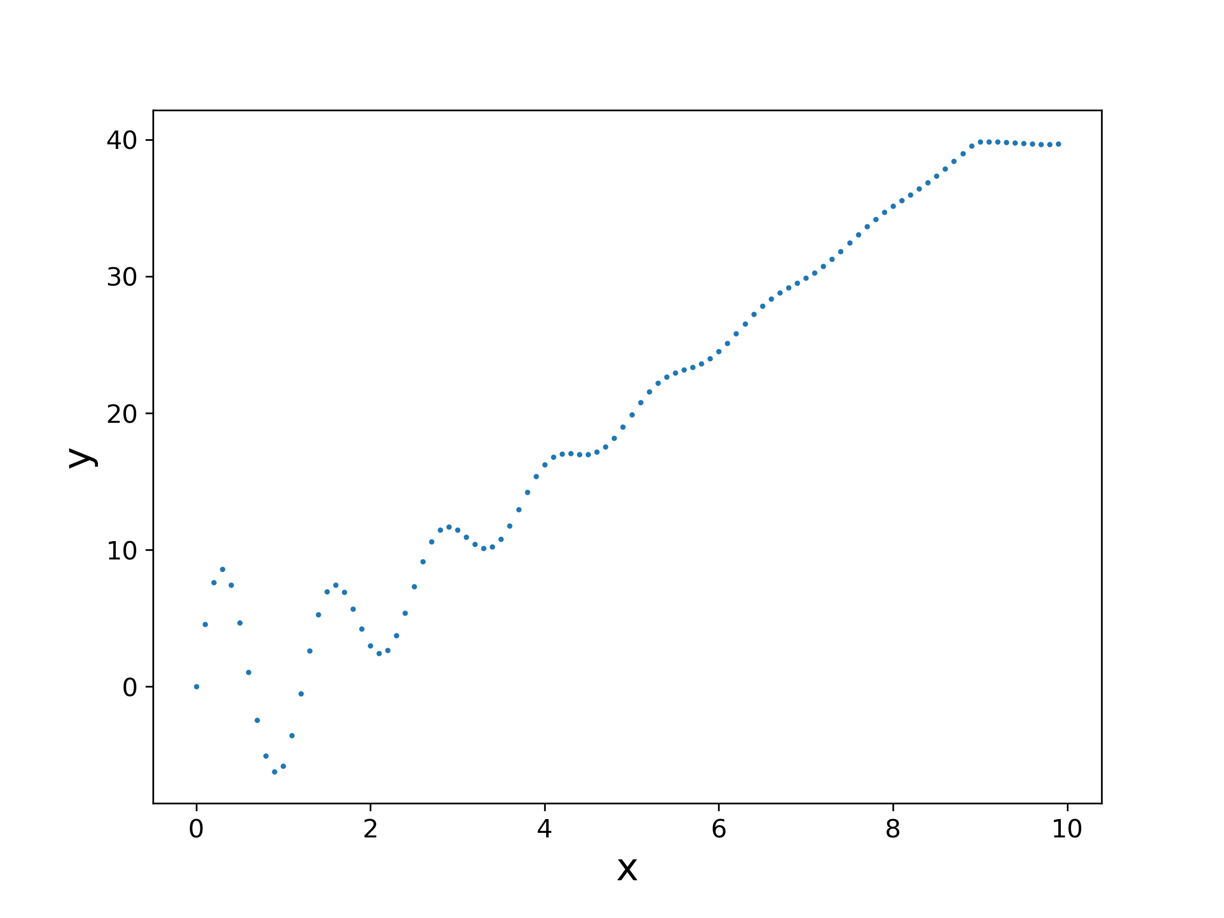
(a) $y(x)=s(x)+d(x)$

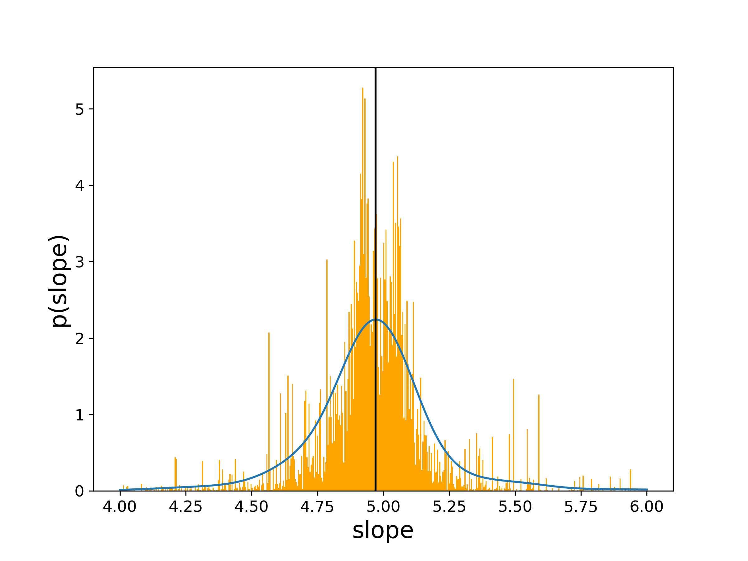
(b) Weighted slope histogram with the KD estimator

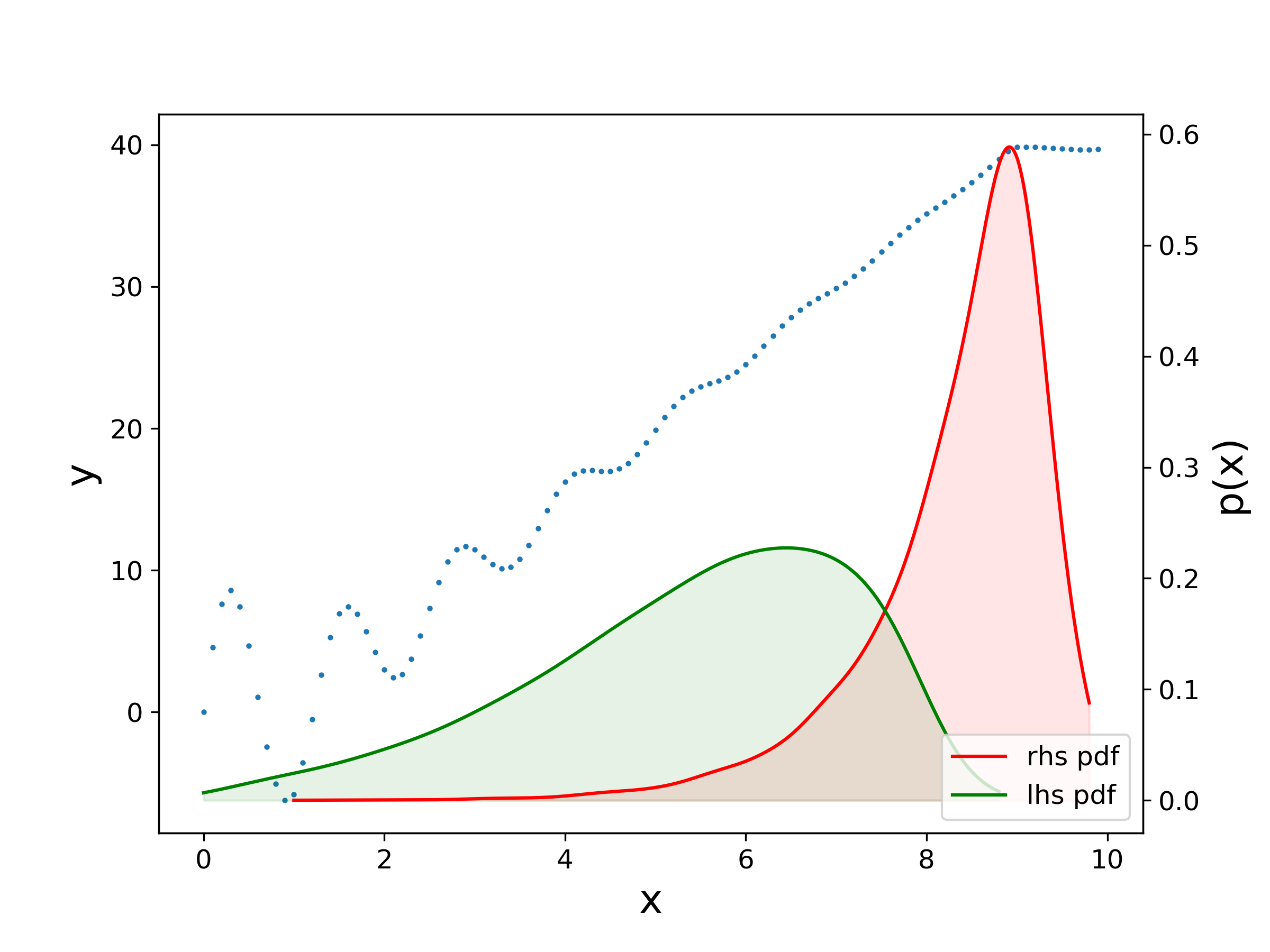
(c) Weighted distributions of interval endpoints

Figure 1: Extracting a scaling region using an ensemble-based approach. (a) A synthetic example with a linear range that is bounded below by oscillations and above by a flat interval. (b) Distribution of slopes (orange histogram) generated from an ensemble of fits in different intervals of this plot, weighted by the inverse square of the fitting error. A kernel density estimation for the probability density is shown in blue, with its mode marked by the black line. The horizontal axis is clipped to [4,6]. (c) Probability distributions of the interval endpoints $[x_{l},x_{r}]$ from the ensemble, with the same weighting as (b).

These data are obtained from a function $y(x)=s(x)+d(x)$, where $s(x)$ is piecewise linear, with slope $5$ in the region $1\leq x\leq 9$:

$$s(x)=\begin{cases}0,&x<1\\ 5x-5,&1\leq x\leq 9\\ 40,&9<x\end{cases}.$$

This function exhibits a scaling region in the range $[1,9]$ that is bounded by intervals with zero slope: a shape that is similar to what is often seen in computations of dynamical invariants even for well-sampled, noise-free data. To make the problem less trivial, we add a damped oscillation,

$$d(x)=10\ e^{-0.5x}\sin(5x),$$

to $s(x)$. The data set for this example is taken to be $y(x)$ on $[0,10)$ with a sampling interval $\Delta x=0.1$.

To find a scaling region in a diagram like Fig. 1(a), one would normally choose two points—markers $x_{l}$ and $x_{r}$ for the bounds of the linear region—then fit a line to the interval $[x_{l},x_{r}]$. A primary challenge is to identify the appropriate interval. For Fig. 1(a), the range $7\leq x\leq 9$ appears to be linear, but should this range extend to smaller $x$? One could certainly argue that the lower boundary could be $x_{l}=6$ instead of $7$, but it would be harder to defend a choice of $x_{l}\leq 4$ because of the growing oscillations.

Several approaches have been proposed for formalizing this procedure in the context of the largest Lyapunov exponent (LLE) problem. These include what Ref. [Zhou and Wang, 2018] calls the “small data method”—used, for example, in Ref. [Rosenstein, Collins, and De Luca, 1993]—which is efficient but suffers from the subjectivity problem described above; an object searching method of the “maximum nonfluctuant," which often reports a local optimal solution Yongfeng et al. (2012); and a fuzzy C-means clustering approach Shuang et al. (2016), which also has limitations since the number of clusters must be pre-specified by the user.

Our approach formalizes the selection of a scaling interval by first choosing all possible “sensible” combinations of left- and right-hand-side marker pairs. Specifically, given a sequence of data points at $\{x_{j},\;j=1..N\}$, we choose $x_{l}$ and $x_{r}$ such that

$$r-l>n,$$ (1)

so that the left marker $x_{l}$ must be below the right one ($x_{r}$) and there must also be at least $n+1$ data points on which to perform the linear fit. For each pair $[x_{l},x_{r}]$, we perform a least-squares fit using the data bounded by the pair to compute both the slope and the least-squares fit error. To suppress the influence of intervals with poor fits, we construct a histogram of their slopes, weighting the frequency of each directly by the length of the fit and inversely by the square of the associated fitting error. Finally, we use a kernel density estimator to fit a smooth probability density function (PDF) to the histogram. The details are presented in Appendix A, along with a discussion of the choices for $n$ and the exponents associated with the fit width and the fitting error (which are set to 1 and 2, respectively, in the experiments reported here).

A central claim in this paper is that the resulting distribution contains useful information about the existence, extent, and slope of the scaling region. The slopes for which the PDF is large represent estimates that not only occur for more intervals in the graph, but also that are longer and have lower fit errors. In particular, we conjecture that the mode of this distribution gives the best estimate of the slope of the scaling region: i.e., a value with low error that persists across multiple choices for the position of the interval. More formally, most intervals $[x_{l},x_{r}]$ that result in slopes near the mode of the PDF (within full width half maximum Weik (2001)) correspond to high-quality fits of regions in the graph whose bounds lie within the interval of the scaling region. If the graph has a single scaling region, the PDF will be unimodal; a narrower peak indicates that the majority of high quality fits lie closer to the mode. Broad peaks and multimodal distributions might arise for multiple reasons, including noise; we address these issues in §III.

For the example in Fig. 1, there are $N=100$ data points and we set $n=10$ so the ensemble of endpoints has $4005$ elements. The resulting weighted slope distribution is unimodal, as shown in panel (b), with mode $4.97$—not too far from the expected slope of 5.0. To provide a confidence interval around this estimate, we compute three quantities:

1. the full width half maximum ($FWHM$) of the PDF around the mode;

2. the fraction, $p_{FWHM}$, of ensemble members that are within the $FWHM$;

3. the standard deviation, $\sigma$, for the slopes of the ensemble members within the $FWHM$.

For the example in Fig. 1, we obtain

$$FWHM=0.36,\quad p_{FWHM}=0.67,\quad\mbox{and }\sigma=0.11.$$

That is, we estimate the slope of the scaling region as $4.97$ $\pm$ $0.11$, noting that fully $67\%$ of the estimated values are within $\pm 0.18$. These error estimates quantify the shape of the peak, and give assurance that the diagram does indeed contain a scaling region.

The method also can estimate the boundaries of the scaling region. To do this, we compute secondary distributions using the positions of the left-hand and right-hand side markers. Since we choose all possible pairs, subject to the constraint (1), the probability densities of the resulting histograms will decrease linearly for $x_{l}$ and grow linearly for $x_{r}$ from left to right. To penalize poor fits, we again scale the frequency for each point in these secondary histograms directly by the length and inversely by the square of the error of the corresponding fit. The resulting PDFs for the synthetic example of Fig. 1(a) are shown in panel (c). The modes of the LHS and RHS histograms fall at $x_{l}=6.45$ and $x_{r}=8.92$, respectively. These align neatly with what an observer might choose as the endpoints of the putative scaling region in Fig. 1(a). Note that the $x_{l}$ distribution is wider with a relatively lower peak, whereas the $x_{r}$ distribution is narrower and taller. This indicates that we can be more certain about the position of the right endpoint than we are about the left one. There is more flexibility in choosing $x_{l}$ than $x_{r}$.

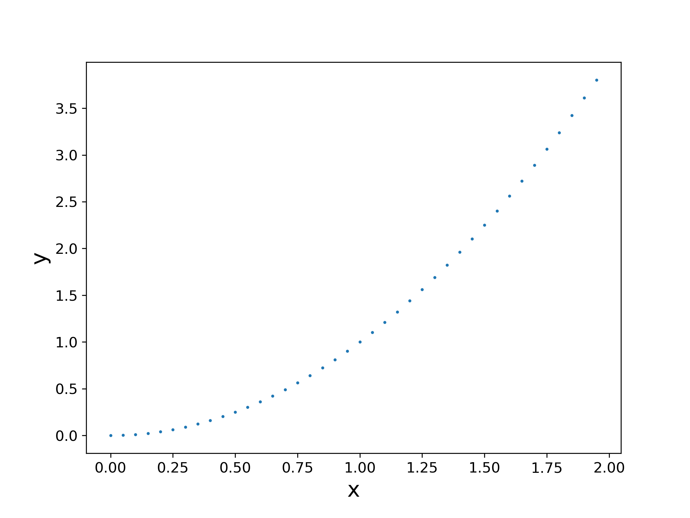
(a) $y(x)=x^{2}$

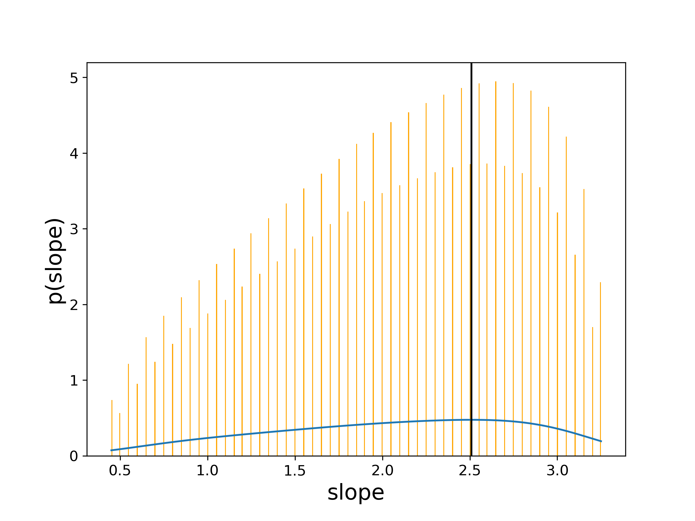
(b) Weighted slope histogram with the KD estimator

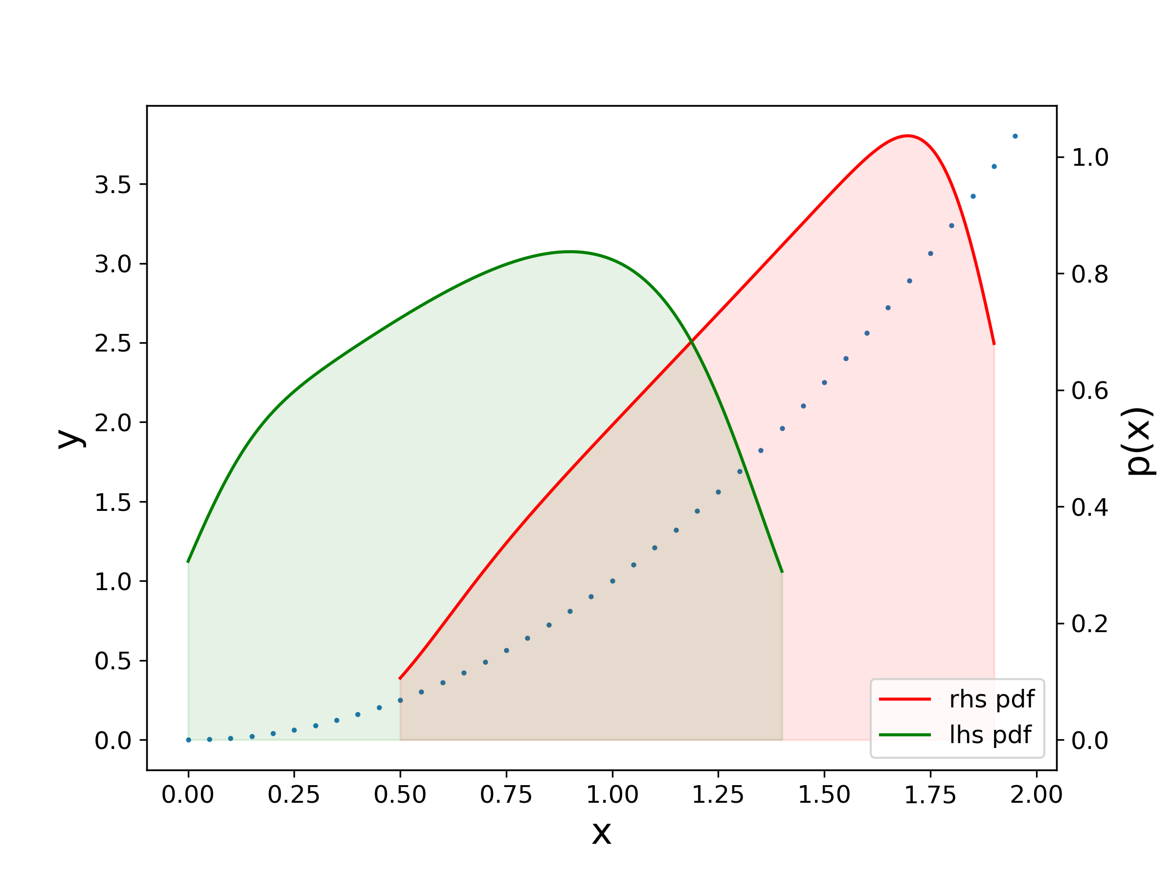
(c) Weighted distributions of interval endpoints

Figure 2: Estimating the scaling region of a quadratic function.

To test our ensemble method on a dataset without an obvious scaling region, consider the quadratic function

$$y(x)=x^{2}\\ .$$

We choose the range $x\in[0,2]$ and a sampling interval $\Delta x=0.05$. A graph of resulting function, Fig. 2(a), of course has no straight regions; though, one might imagine that the curve becomes nearly linear near the top of the range even though the actual slope grows linearly with $x$. The slope distribution, shown in Fig. 2(b), has mode

$$2.51\pm 0.63\quad(FWHM=2.18\mbox{ and }p_{FWHM}=0.89),$$

and as the endpoint distributions in panel (c) show, this corresponds to the interval $[x_{l},x_{r}]=[0.90,1.70]$. However, the large width of the slope distribution and the correspondingly high magnitude of $\sigma$ convey little confidence as to the existence of a scaling region. This shows that the error statistics and the $FWHM$ can be useful indicators as to whether or not a scaling region is present. A high error estimate and/or a high FWHM contraindicates a scaling region.

In the case of the two simple examples above, scaling regions imply simple linear relationships between the independent and dependent variables. Our technique can just as well be applied to plots with suitably transformed axes—like the log-linear or log-log axes involved in the computation of many dynamical invariants—as we demonstrate next by computing the dimension of a fractal.

The box-counting dimension, $d_{box}$, is the growth rate of the number $N(\epsilon)$ of boxes of size $\epsilon$ that cover a set:

$$N(\epsilon)\propto\epsilon^{-d_{box}}.$$ (2)

In practice, $d_{box}$ is estimated by computing the slope of the graph of $\ln\ N(\epsilon)$ versus $\ln\tfrac{1}{\epsilon}$.

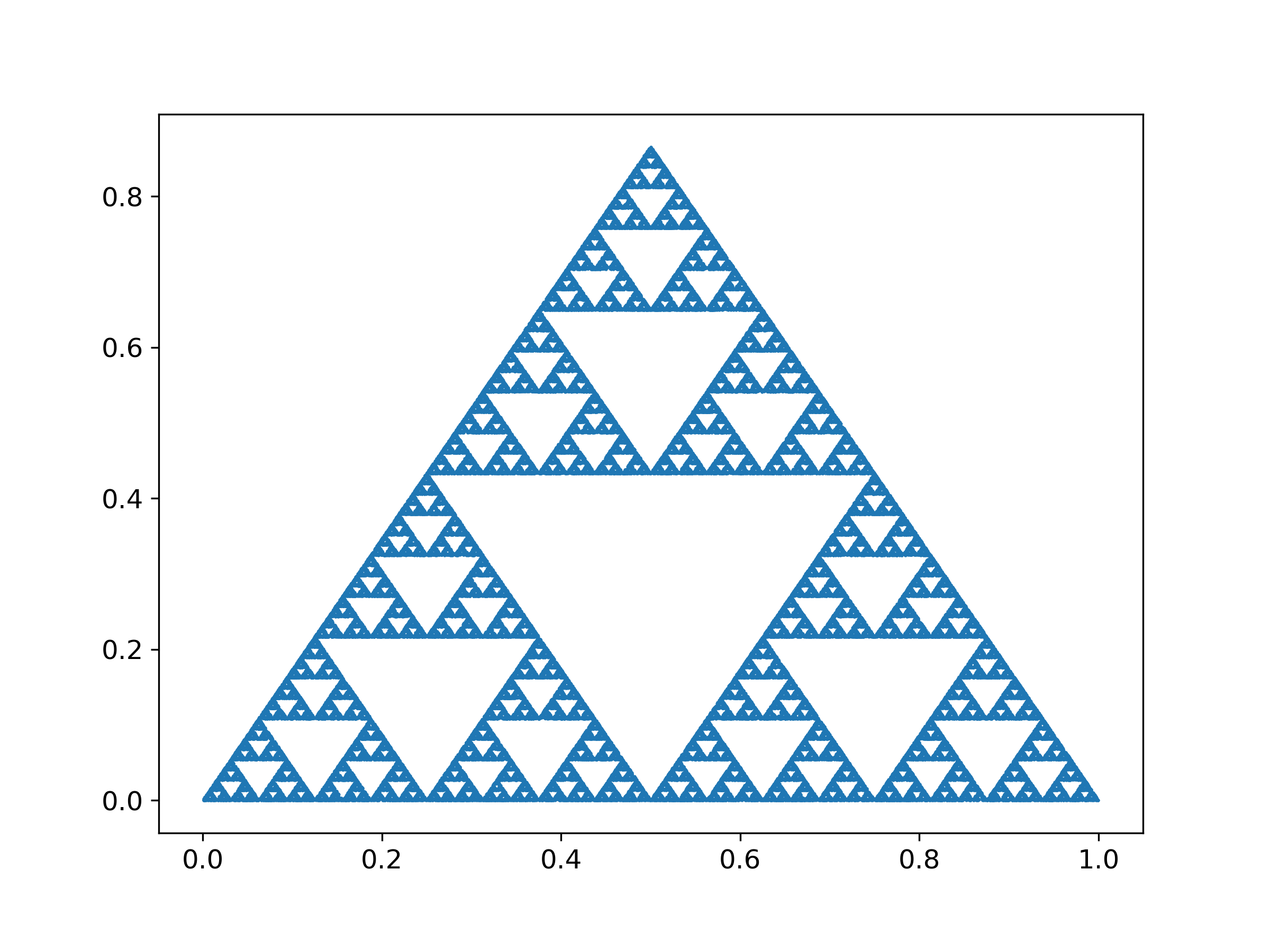
(a) 100,000 points on the Sierpinski Triangle

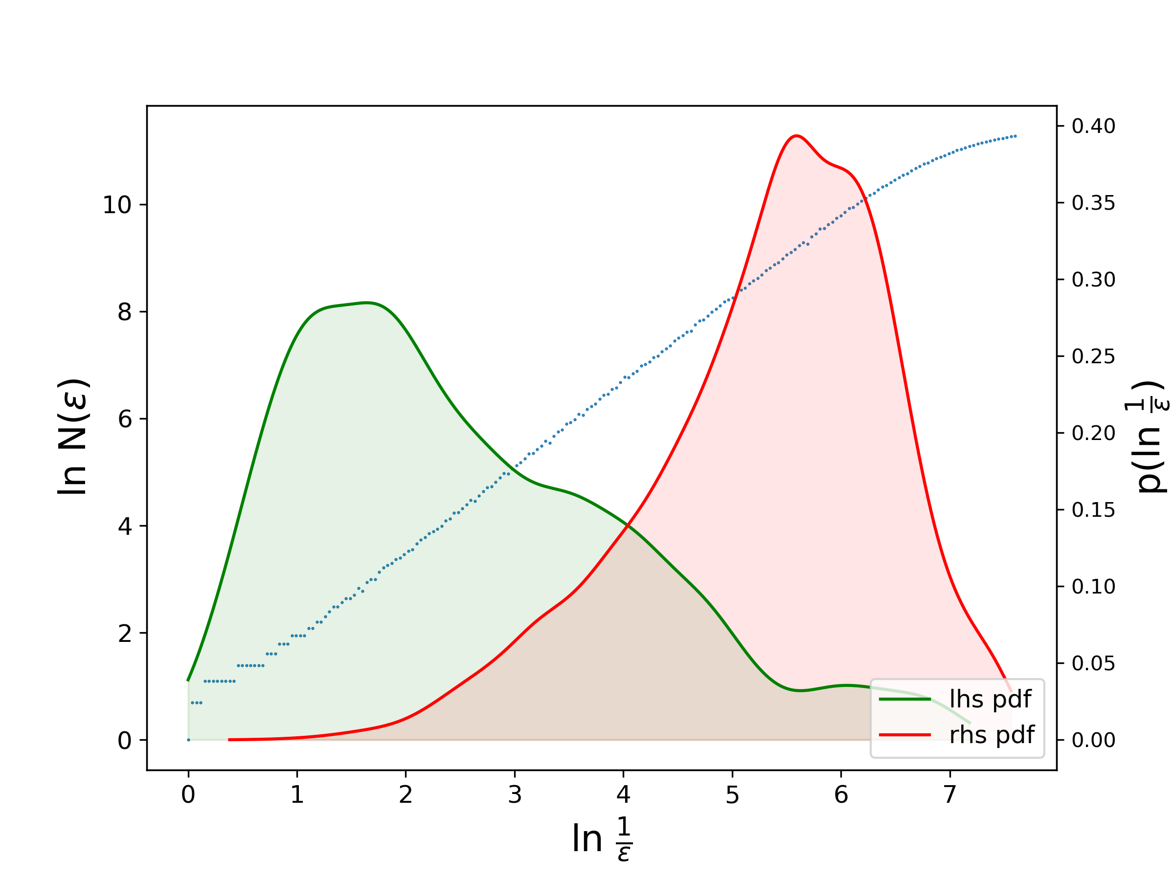
(b) Log-log plot of $N(\epsilon)$

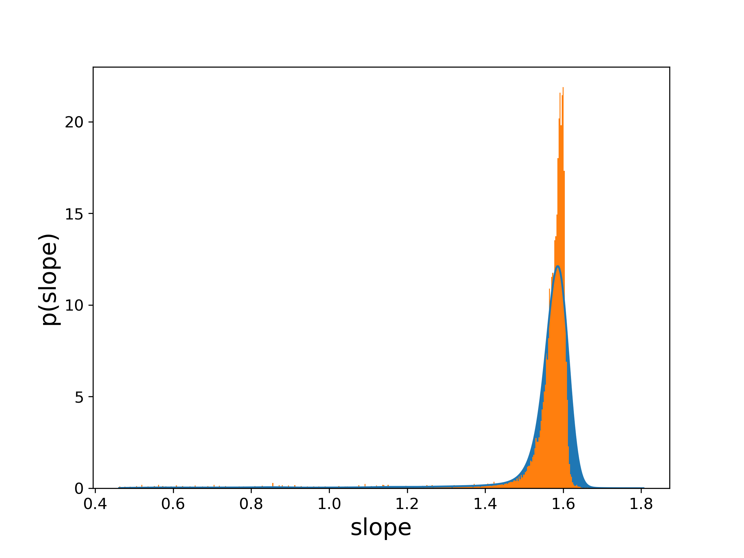
(c) Weighted slope distribution

Figure 3: Estimating the box-counting dimension of the Sierpinski Triangle.

As an example, we consider the equilateral Sierpinski triangle of side one, generating a set of $10^{5}$ points using an iterated function system Peitgen, Juergens, and Saupe (1992) to obtain Fig. 3(a). A log-log plot of $N(\epsilon)$ for this data set is shown in Fig. 3(b) and the resulting slope distribution is shown in Fig. 3(c). The mode of this distribution falls at $1.585$ $\pm$ $0.020$, where—as before—the error is the estimate $\sigma$. This is close to the true dimension $\frac{\ln 3}{\ln 2}$ $\approx$ $1.585$. This peak is narrow, with $FWHM=0.07$, though $p_{FWHM}=0.68$, similar to the first example. Thus about $70\%$ of the weighted fits lie within $\pm 0.035$ of the estimated slope, strengthening confidence in the estimate. The small periodic oscillations in the curve in Fig. 3(b) are due to the self-similarity of the fractal. Note that the linear growth saturates when $\ln\tfrac{1}{\epsilon}<0.5$, the point at which the box size becomes comparable to the diameter of the set. Neither of these effects significantly influences the mode of the slope distribution. For this example, the LHS and RHS distributions in panel (b) have similar widths, with modes $x_{l}=1.64$ and $x_{r}=5.59$, respectively.

The examples of this section show that the ensemble-based method effectively selects an appropriate scaling region—if one exists—and is able to exclude artifacts near the edges of the data.

III Applications to Dynamical Systems

In this section, we apply this scaling region identification and characterization method to calculations of two dynamical invariants—the correlation dimension (§III.1) and the Lyapunov exponent (§III.2)—for two well-known examples, the Lorenz system and the driven, damped pendulum. We also explore the effects of noise (§III.1.3) and the selection of embedding parameters for delay reconstructions (§III.1.4).

III.1 Correlation Dimension

Correlation dimension, one of the most common and useful dynamical invariants, can be calculated using the Grassberger-Procaccia algorithm Grassberger and Procaccia (2004, 1983). Given a set of points that sample an object, such as an attractor of a dynamical system, this algorithm estimates the average number of points in an $\epsilon$-neighborhood of a given point, $C(\epsilon)$. For an attractor of correlation dimension $d_{2}$, this scales with $\epsilon$ as

$$C(\epsilon)\propto\epsilon^{d_{2}}.$$ (3)

Estimating $d_{2}$ is therefore equivalent to finding a scaling region in the log-log plot of $C(\epsilon)$ versus $\epsilon$ Grassberger and Procaccia (1983).

In this section, we use d2, the TISEAN Kantz and Schreiber (1997) implementation, which outputs estimates of $C(\epsilon)$ for a range of $\epsilon$ values. We apply our ensemble-based method to a graph of log $C(\epsilon)$ versus log $\epsilon$ and identify the mode of the resulting slope distribution to obtain an estimate of the correlation dimension of the data set. When the slope distribution is multi-modal, our method can also reveal the existence of potential scaling regions for different ranges of $\epsilon$, some of which may not be obvious on first observation. This analysis, then, not only yields values for the slope and extent of the scaling region; it also provides insight into the geometry of the dynamics, the details of the Grassberger-Procaccia algorithm, and the interactions between the two.

III.1.1 Lorenz

We start with the canonical Lorenz system:

$$\dot{x} =\sigma(y-x),$$

$$\dot{y} =x(\rho-z)-y,$$

$$\dot{z} =xy-\beta z,$$

with $\sigma=10$, $\beta=\frac{8}{3}$, and $\rho=28$ Lorenz (1963). We generate a trajectory from the initial condition $(0,1,1.05)$ using a fourth-order Runge-Kutta algorithm for $10^{5}$ points with a fixed time step $\Delta t=0.01$, discarding the first $10^{4}$ points to remove the transient, to get a total trajectory length of 90,000 points. The chosen initial condition lies in the basin of the chaotic attractor and the discarded length is sufficient to remove any transient effects. Figure 4(a) shows a log-log plot of $C(\epsilon)$ versus $\epsilon$ produced by the d2 algorithm.

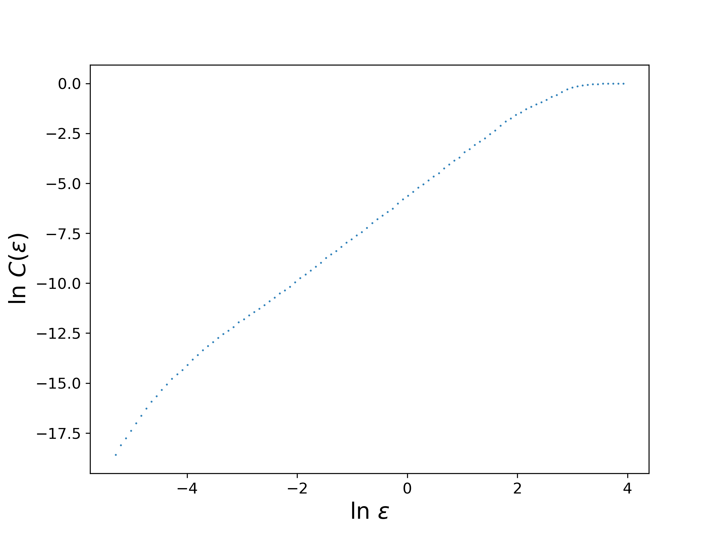
(a) Correlation sum calculations

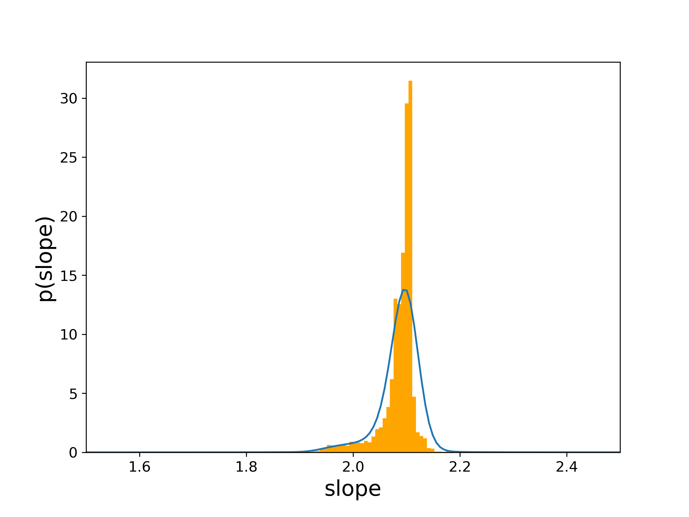
(b) Weighted slope distribution

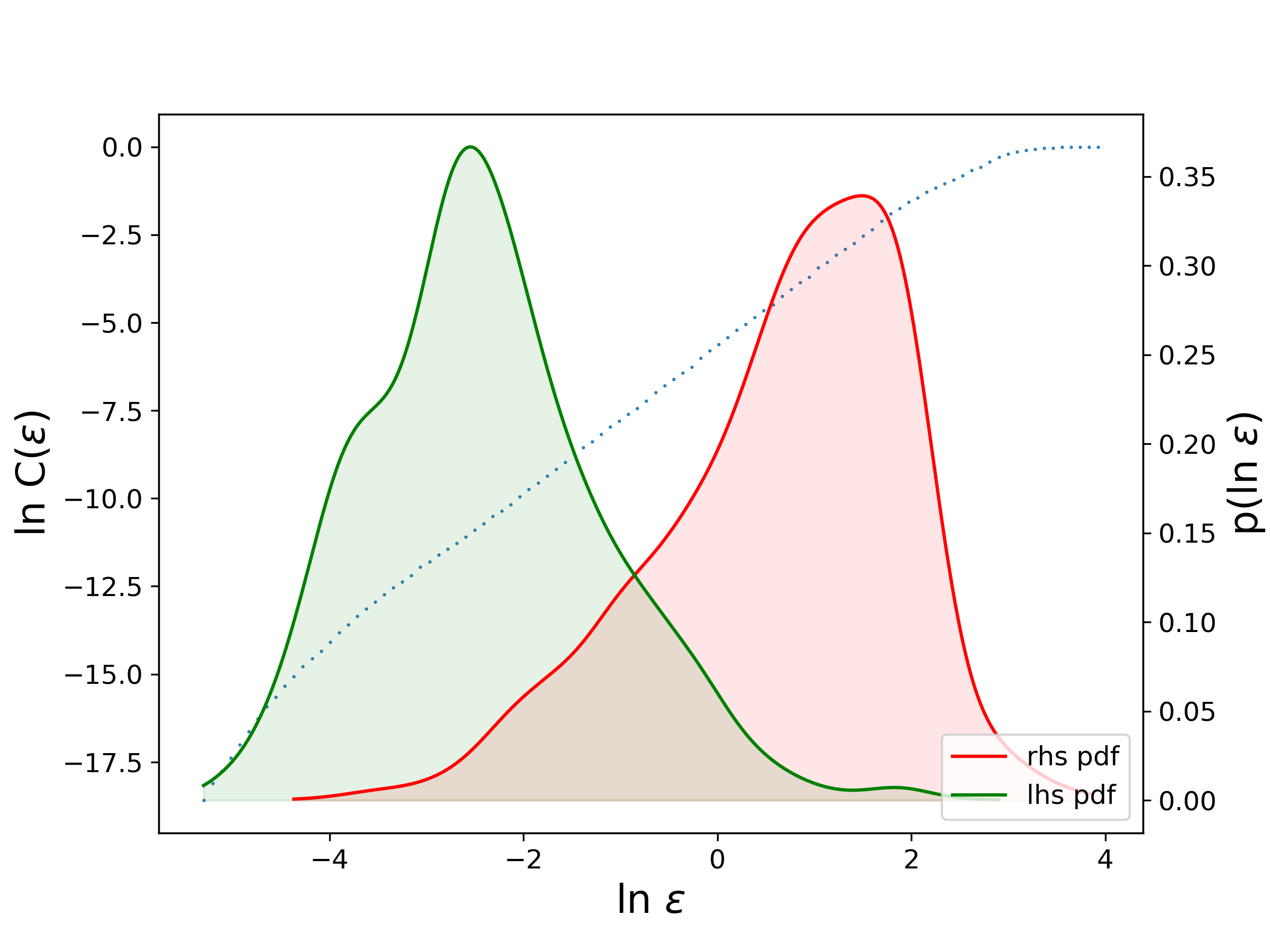
(c) Weighted distributions of interval endpoints

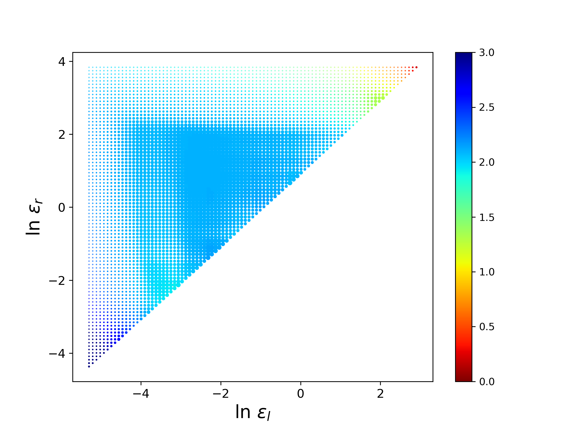
(d) Heatmap of the endpoint ensemble

Figure 4: Estimating the correlation dimension of the Lorenz attractor

To the eye, this graph appears to contain a scaling region in the approximate range $[\ln\epsilon_{l},\ln\epsilon_{r}]=[-3,2]$. As in the box-counting dimension example in §II, the curve flattens when $\epsilon$ is larger than the diameter of the attractor, since $C(\epsilon)$ will not change when $\epsilon$ increases beyond this point. Since the diameter of the Lorenz attractor is $25.5$, this flattening occurs for $\ln\epsilon>\ln(25.5)\approx 3.2$.

Figures 4(b) and (c) show the results of our ensemble-based approach. The mode of the slope PDF is

$$2.09\pm 0.02\quad(FWHM=0.06\mbox{ and }p_{FWHM}=0.69);$$

this gives an estimate for the correlation dimension for the Lorenz attractor that agrees with the accepted range, $2.06-2.16$ Viswanath (2004); Martínez, Domínguez-Tenreiro, and Roy (1993). The PDFs of the LHS and RHS markers in Fig. 4(c) have modes $\ln\epsilon_{l}=-2.6$ and $\ln\epsilon_{r}=1.5$, respectively. Estimates of both endpoints by our algorithm are close to the informal ones, although slightly on the conversative side. In other words, our method can indeed effectively formalize the task of identifying both the existence and the extent of scaling regions.

The endpoint distributions can be broken down further in the heatmap-style scatter plot of Fig. 4(d) to reveal additional details. Each dot represents a single element of the ensemble: i.e., a fit for a particular interval $[\ln\epsilon_{l},\ln\epsilon_{r}]$. Its color encodes the slope and its radius is scaled by the fitting weight. If samples come from intervals that are close, the associated dots will be nearby; if these have low error, the dots will be large and their effective density will be high. Note that the domain of panel (d) is a triangle since $\epsilon_{l}<\epsilon_{r}$ by (1).

This visualization provides an effective way to identify scaling region ranges that produce similar slope estimates: long scaling regions will manifest as large regions of similarly colored points. Fig. 4(d) shows such a triangular high-density region in blue (slope $\approx$ 2.0), above the diagonal, bounded from the left by $\ln\epsilon_{l}\approx-4$, and from above by $\ln\epsilon_{r}\approx 2$. This clearly corresponds to the primary scaling region in Fig. 4(a) and the corresponding mode in panel (b). This heatmap can reveal other, shorter scaling regions. Indeed, panel (d) shows other clusters of similarly colored dots that are somewhat larger than the dots from neighboring regions: e.g., the green cluster for $\ln\epsilon_{l}\approx 2$ and $\ln\epsilon_{r}\approx 3$, with a slope near $1.5$. Close examination of the original curve in Fig. 4(a) reveals a small straight segment in the interval $[2,3]$. This, not immediately apparent, feature stands out quite clearly in the distribution visualization. Two much smaller scaling regions at the two ends of panel (a) are also brought out by this representation: the interval of slope $\approx$ 3.0 for small $\epsilon$ (the dark blue cluster at the lower left corner of the scatter plot) and the zero slope for large $\epsilon$ (the red cluster at the upper right corner).

III.1.2 Pendulum

As a second example, we study the driven, damped pendulum:

$$\begin{split}\dot{\theta}&=\omega,\\ \dot{\omega}&=-\beta\omega-\nu_{0}^{2}\sin(\theta)+A\cos(\alpha\ t),\\ \end{split}$$ (4)

where the natural frequency is $\nu_{0}=98$, the damping coefficient is $\beta=2.5$, and the driving force has amplitude $A=91$ and frequency $\alpha=0.75\nu_{0}$. The coordinates of the three-dimensional extended phase space $\mathbb{T}^{2}\times\mathbb{R}$ are the angle $\theta$, the time $t$, and the angular velocity $\omega$. We generate a trajectory for this system using a fourth-order Runge-Kutta algorithm with initial condition $(3.14,0,50)$ for $1.1\times 10^{6}$ points with fixed time step $0.001$, discarding the first $10^{5}$ points to remove the transient, resulting in a final time series of length one million. To avoid issues with periodicity in $\theta$ and $t$, we project the time series from $\mathbb{T}^{2}\times{\mathbb{R}}$ onto $(\sin(\theta),\sin(\alpha t),\omega)\in\mathbb{{\mathbb{R}}}^{3}$. The resulting trajectory is shown in Fig. 5. Note that the attractor has the bound $|\omega|\leq 24.88$, but that the range of the other two variables is $[-1,1]$ due to the sinusoidal transformation.

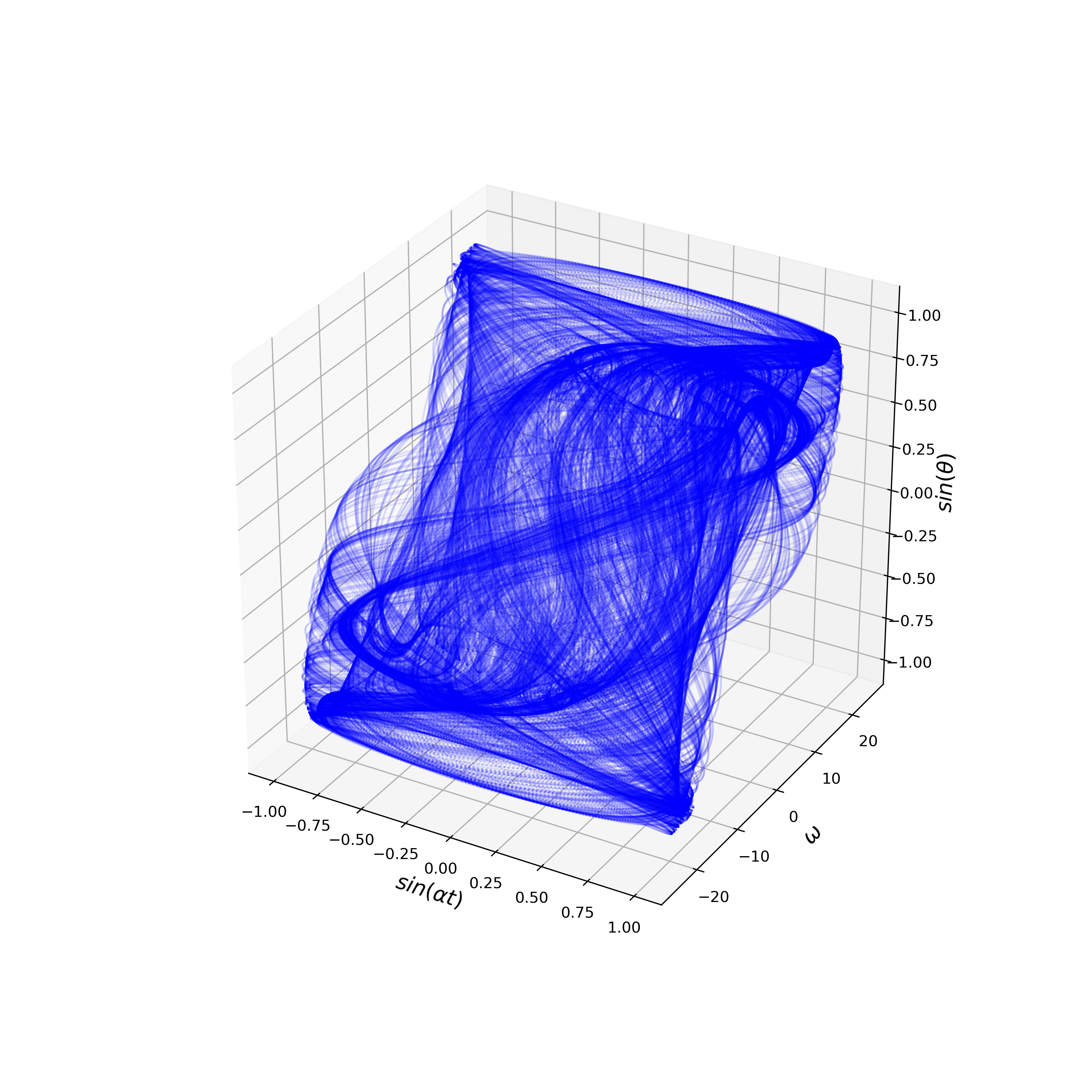
Figure 5: A trajectory of the driven, damped pendulum (4).

To the eye, results of a d2 calculation on this trajectory, shown in Fig. 6(a), exhibit two apparent scaling regions above and below $\ln\epsilon\approx 1$. The slope distributions produced by our method not only confirm, but also formalize, this observation. The larger peak of the distribution in panel (b) of the figure falls at $d_{2}=2.19\pm 0.09$ ($FWHM$ = 0.32 and $p_{FWHM}=0.53$), which is equivalent to the correlation dimension of the attractor as reported in Ref. [Deshmukh et al., 2020]. Note that, to account for the fact that the distribution is clipped on the right before the density falls below half the peak value, the computation of $FWHM$ uses this as the upper bound. The interval endpoint distributions in panel (c) indicate that the extent of this scaling region is $-2.6<\ln\epsilon<0$. To the eye, $\epsilon_{r}\sim 0.8$ would seem a more-appropriate choice for the RHS endpoint of the scaling region; however, minor oscillations in the interval $\epsilon\in[0,1]$ cause the ensemble-based algorithm to be more conservative and choose $\epsilon_{r}=0$. The presence of a second scaling region in panel (a) for $\ln\epsilon>1$ gives a second mode at the slope $0.94\pm 0.10$ ($FWHM=0.35$ and $p_{FWHM}=0.26$). The secondary peaks in the endpoint distributions in panel (c) suggest an extent of $0.8<\ln\epsilon<2.8$ for this second scaling region, which is consistent with visual inspection of panel (a).

This second scaling region is an artifact of the large aspect ratio of the attractor: only one of the variables, $\omega$, has a range larger than $1$, so when $\epsilon>1$, the effective dimension is one. To test this hypothesis, we rescaled the components of the phase space vectors so that the attractor has equal extent of $[0,1]$ in all three directions (using the -E flag in the TISEAN d2 command) and repeated the d2 calculations. This leads to rescaling of the axis of the $d_{2}$ plot—$\ln\epsilon$ now has the range $[-7,0]$—and causes the second scaling region in the previous results to disappear, leaving a single scaling region $-7<\ln\epsilon<-2$ with slope

$$d_{2}=2.22\pm 0.02\quad(FWHM=0.05,\mbox{ and }p_{FWHM}=0.70).$$

Note that, in addition to resolving the artifact of the second scaling region, this rescaling also reduces the width of the mode and gives a much tighter error bound.

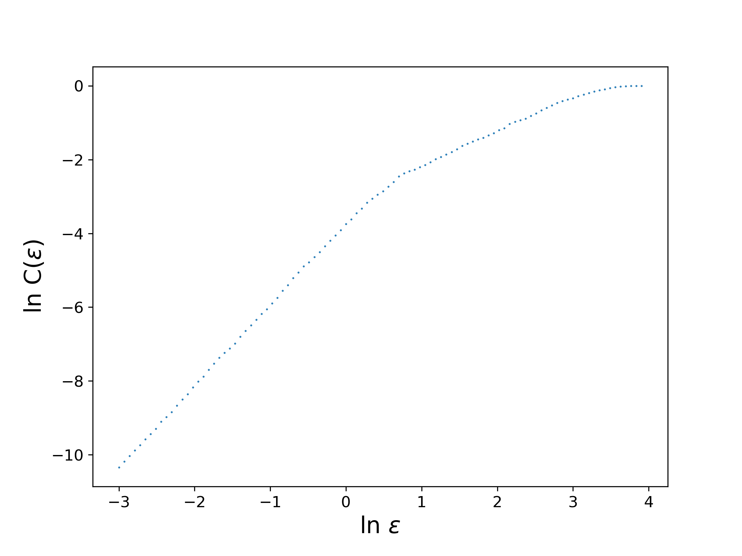
(a) Correlation sum calculations

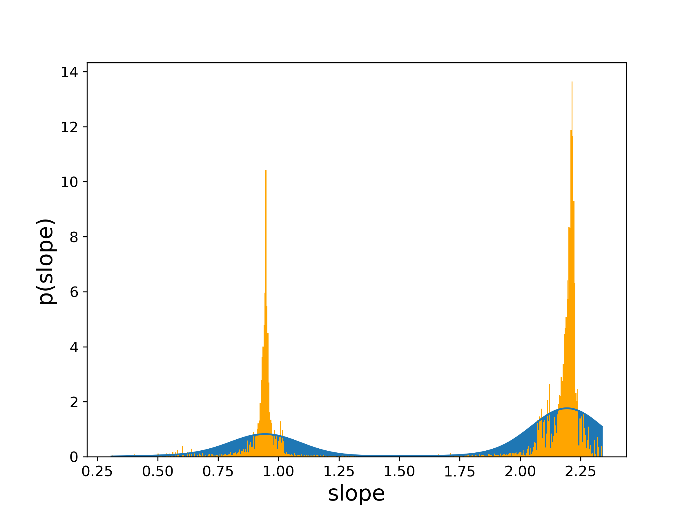
(b) Weighted slope distribution

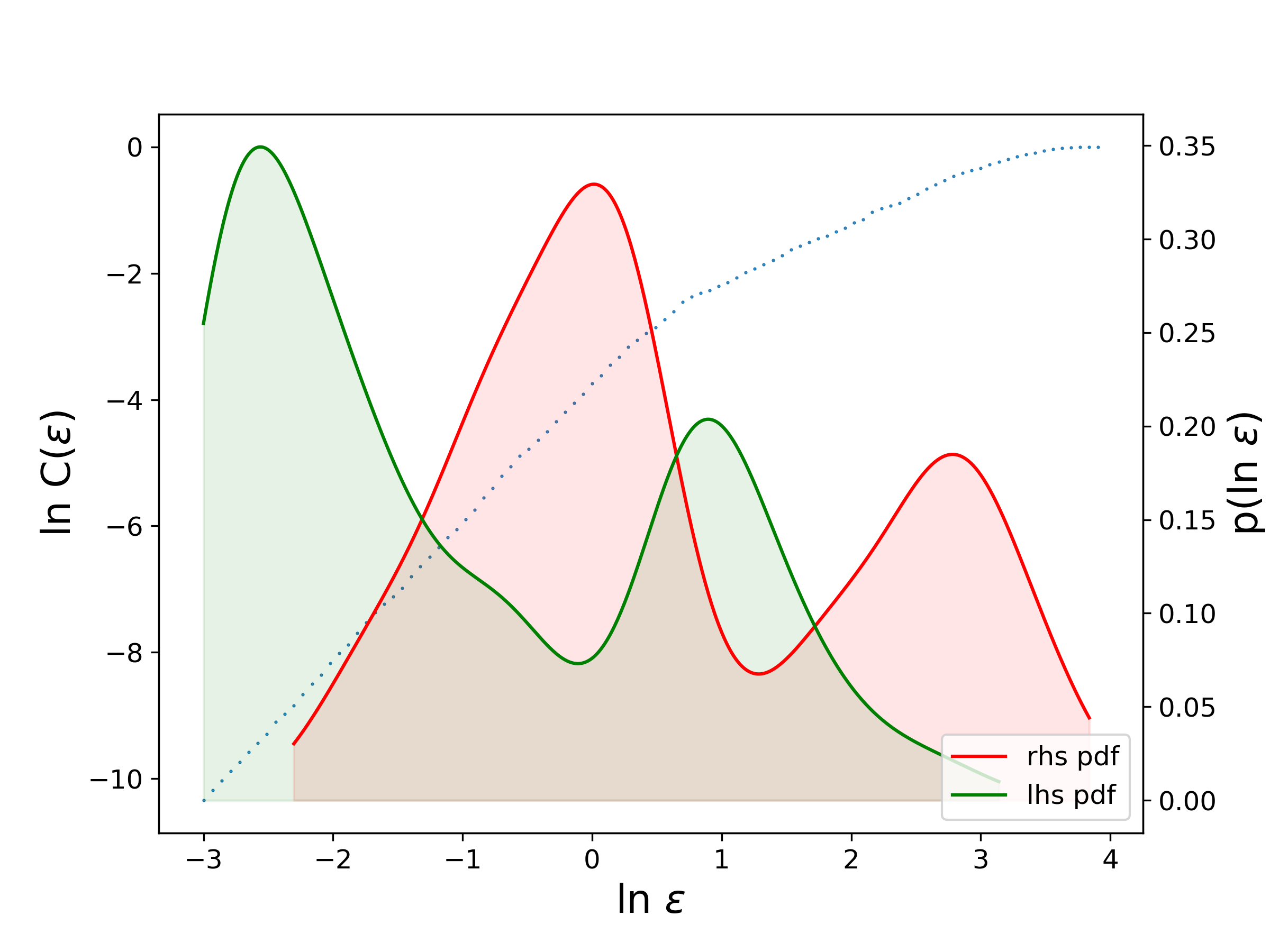
(c) Weighted distributions of interval endpoints with the correlation sum graph from (a) superimposed

Figure 6: Estimating the correlation dimension of the driven, damped pendulum trajectory shown in Fig. 5.

By revealing the existence, the endpoints, and the slopes of different scaling regions in the data, our ensemble-based approach has not only produced an objective estimate for the correlation dimension, but also yielded some insight into the interaction between the d2 algorithm and the attractor geometry.

III.1.3 Noise

Noise is a key challenge for any practical nonlinear time-series analysis method. We explore the effects of measurement noise on our method using the Lorenz trajectory of §III.1.1 by adding uniform noise post facto to each of the three state variables. The noise amplitude in each dimension is proportional to the radius of the attractor in that dimension. The correlation sum $C(\epsilon)$ for a noise amplitude $\delta=0.01$—i.e., $1\%$ of the radius of the attractor in each dimension—is shown in Fig. 7(a).

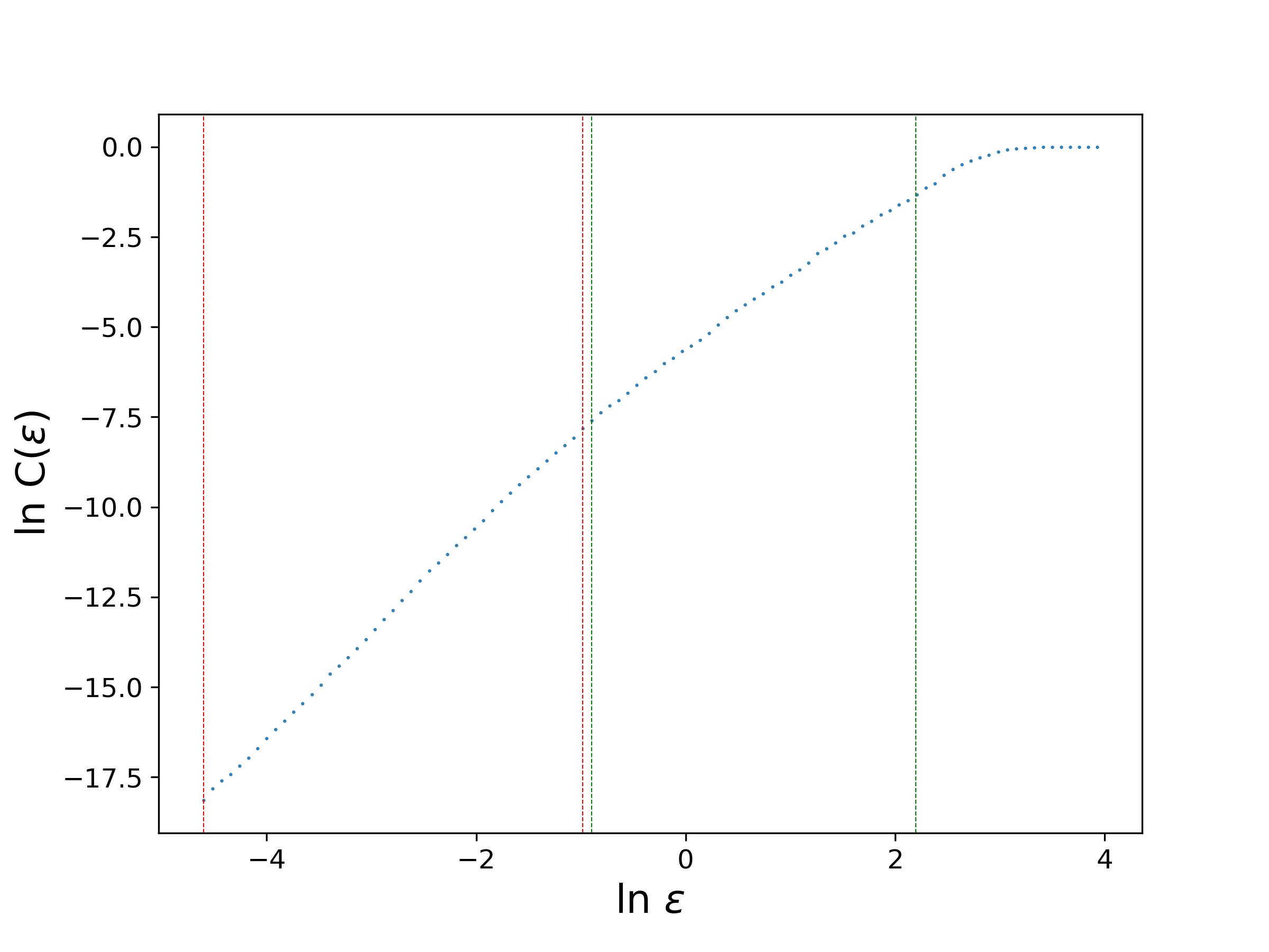
(a) $\delta=0.01$

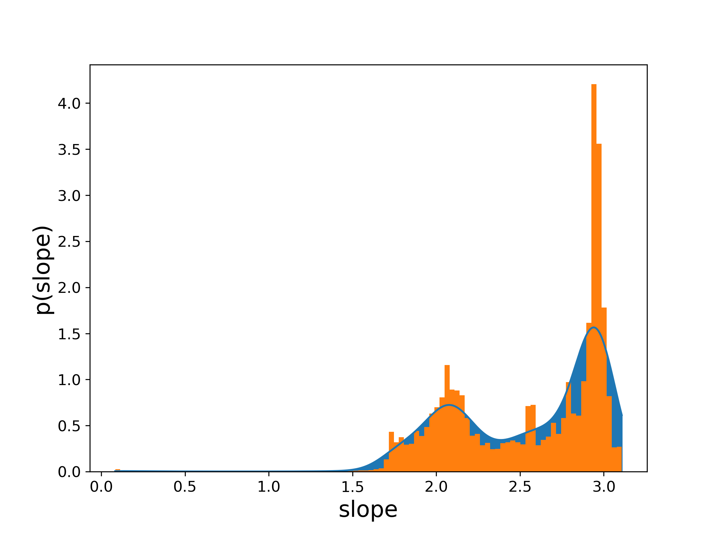
(b) Weighted slope distribution for (a)

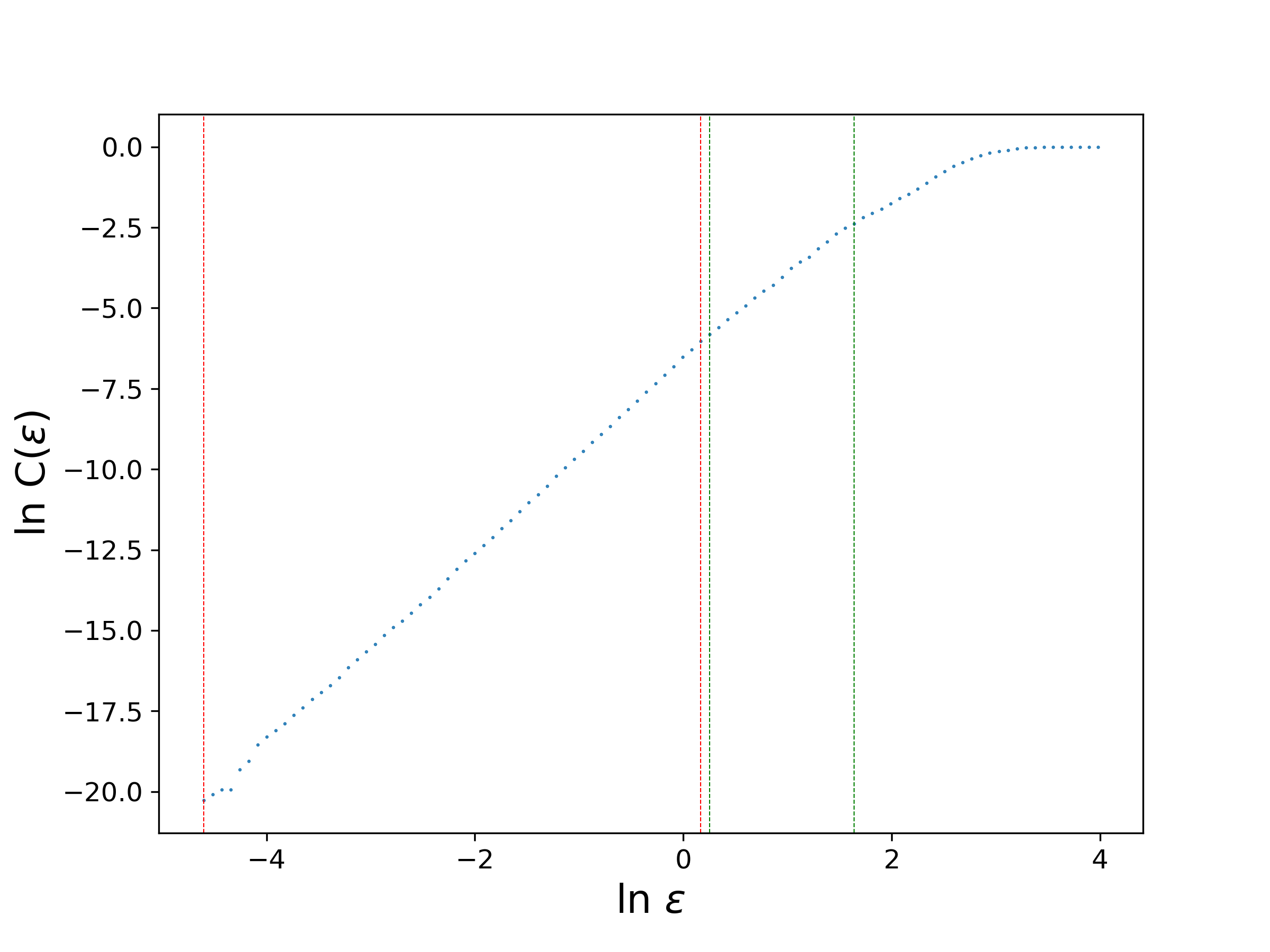
(c) $\delta=0.1$

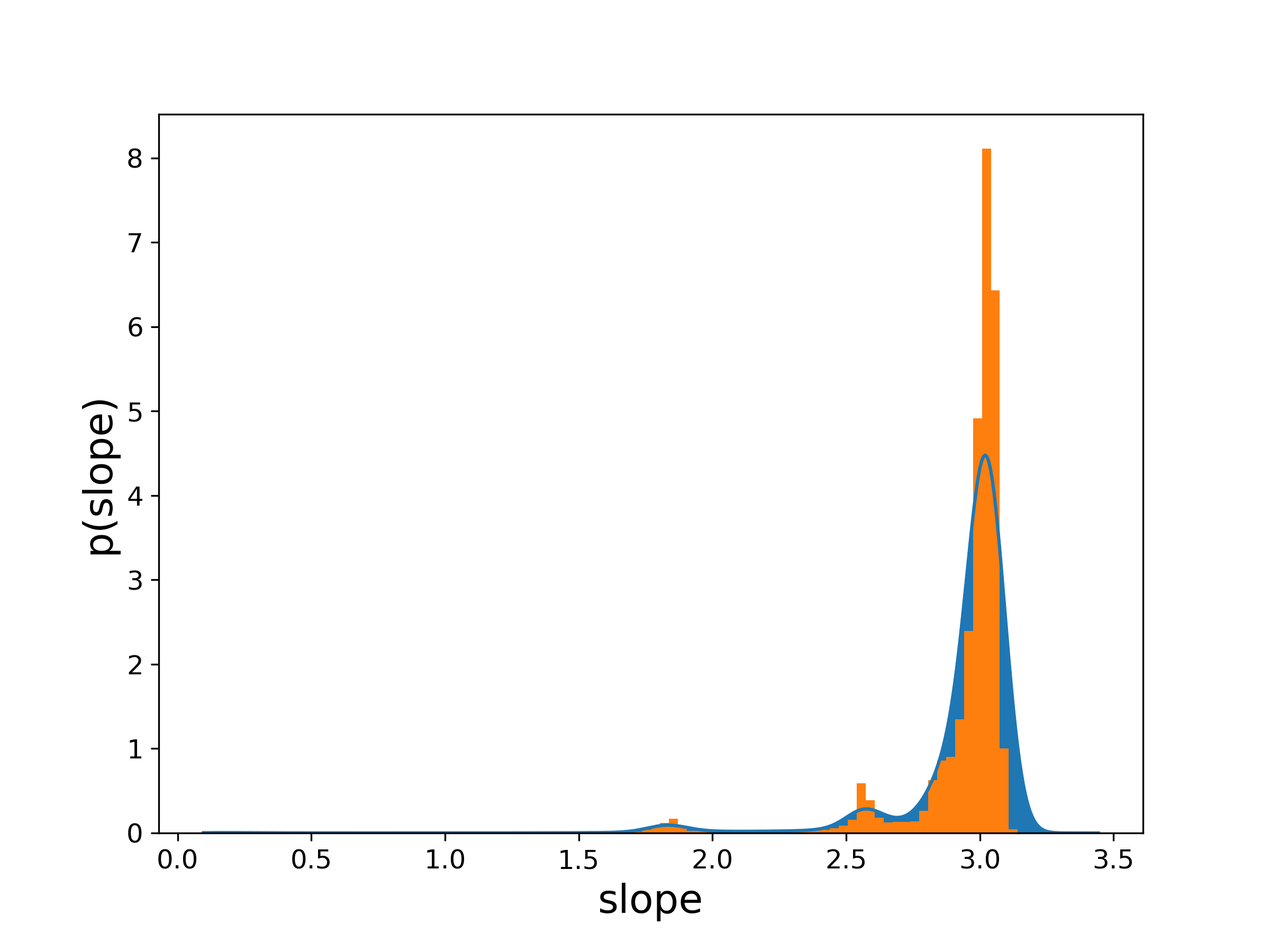
(d) Weighted slope distribution for (c)

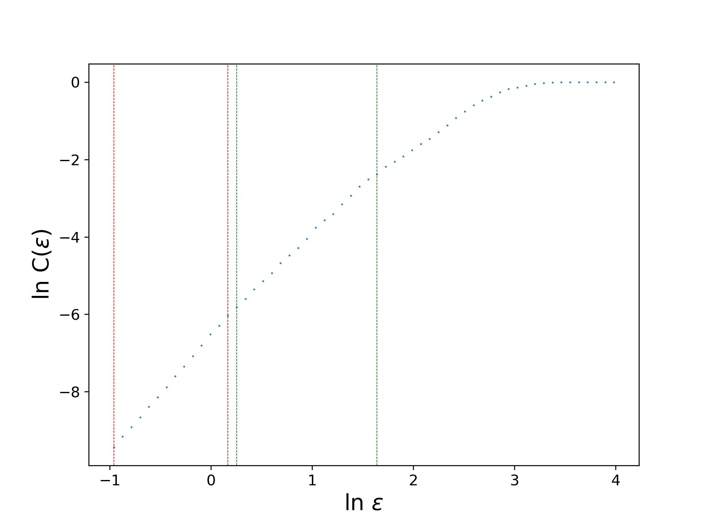
(e) $\delta=0.1$

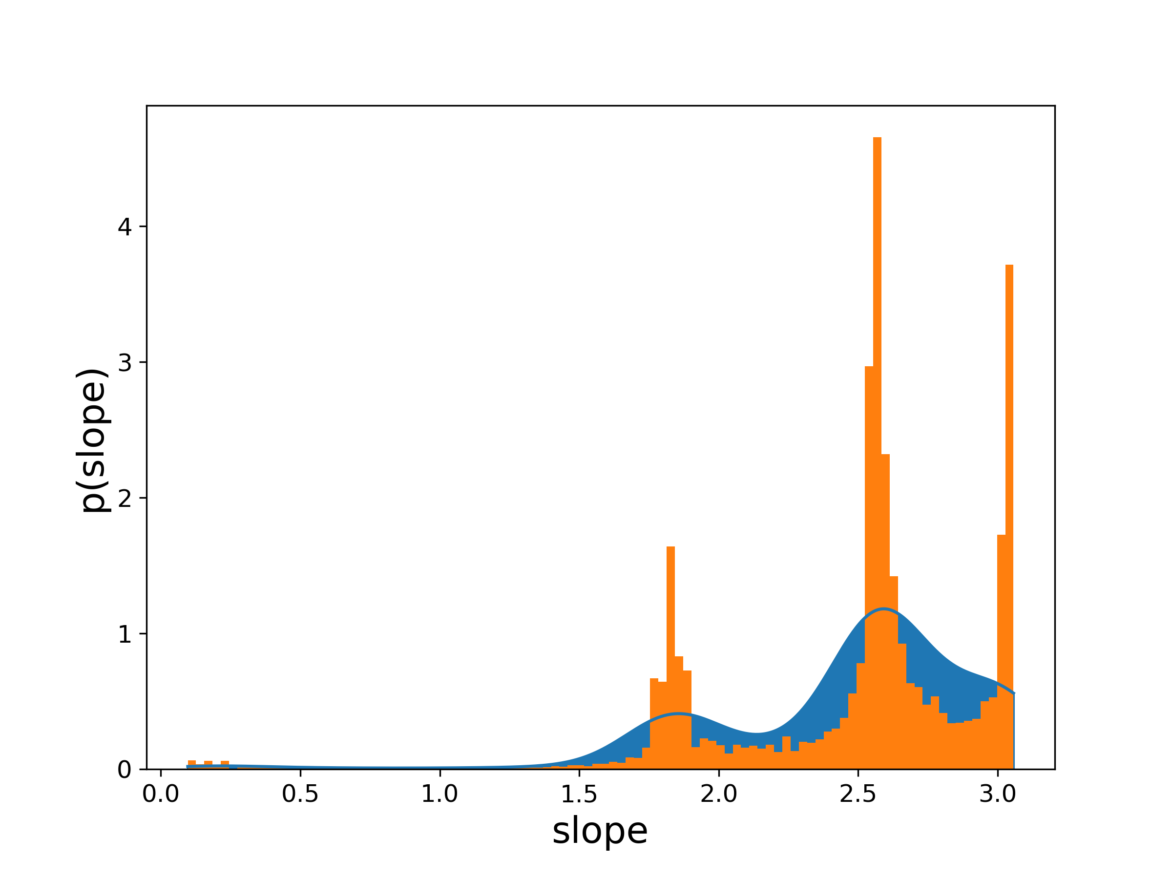
(f) Weighted slope distribution for (e)

Figure 7: Correlation dimension of the Lorenz attractor with added noise $\delta=0.01$ for (a)-(b), and $\delta=0.1$ for (c)-(f). Panels (e)-(f) exclude $\ln\epsilon<-1$. The red markers in (a), (c) and (e) denote scaling regions corresponding to noise while the green markers indicate that for the dynamics.

There appear to be two distinct scaling regions in this plot, above and below a slight knee at $\ln\epsilon\ \approx\ -1$. The slope distribution produced by our method is shown in Fig. 7(b). As in the pendulum example, this distribution is bimodal, indicating the presence of two scaling regions with slopes

$$2.94\pm 0.09 \quad(FWHM=0.33\mbox{ and }p_{FWHM}=0.42),\mbox{ and }$$

$$2.08\pm 0.15 \quad(FWHM=0.51\mbox{ and }p_{FWHM}=0.30),$$

respectively. We claim that these results are consistent with the geometry of the noise and of the dynamics, respectively. The taller peak corresponds to the interval $\ln\epsilon\in[-4.60,-1]$, delineated by red markers in panel (a). Note that the right endpoint of this region is close to $\epsilon_{r}\approx 0.01\times 26$, the maximum extent of the noise. The computed slope of $2.94$ in this interval captures the geometry of a noise cloud in three-dimensional state space. The smaller, secondary peak at $2.08$ reflects the dimension of the attractor for scales larger than the noise, the interval $\ln\epsilon\in[-1,2.2]$ that is bounded by green markers in panel (a).

As the noise level increases, the geometry of the attractor is increasingly obscured (see Fig. 10 in Appendix B). Figures 7(c) and (d) show results for $\delta=0.1$. As one would expect, the right-hand boundary of the lower scaling region is increased, shown as the red markers in panel (c). We observe that $\ln\ \epsilon_{r}\approx 0.16$, near the the noise cloud radius of $1.3$. With this noise level, the slope distribution is nearly unimodal with mode

$$3.02\pm 0.05\quad(FWHM=0.18\mbox{ and }p_{FWHM}=0.65),$$

again reflecting the geometry of the noise. While there appears to be a secondary peak in the slope distribution in panel (d), it is nearly obscured.

Interestingly, the identification of the scaling region due to the noise can be used to refine the calculation and retrieve some information about the dynamical scaling: one simply repeats the slope-distribution calculations using only the data for larger $\epsilon$ values; that is, discarding the values below the noise. Restricting to the interval $[-1.0,4.0]$, gives the curve and the slope distribution shown in panels (e) and (f). In addition to the noise peak near $3.0$, this reveals two additional peaks. The first,

$$2.59\pm 0.20\quad(FWHM=0.68\mbox{ and }p_{FWHM}=0.67),$$

was hinted at by the tail of the distribution in panel (d). This, we conjecture, corresponds to the correlation dimension of the noisy dynamics. The final peak, near $1.8$, corresponds to the smaller scaling region $[2.0,3.0]$ that can be seen in a heatmap-style scatter plot (not shown). The validity of this region can be easily confirmed by further limiting the ensemble to the interval $\ln\epsilon\in[1.0,4.0]$ which then gives a single mode at $1.83$. Note that this region corresponds to a smaller scaling region that was also seen in the noiseless case: the small green cluster in Fig. 4(d).

The ability of the ensemble-based slope distribution method to reveal secondary scaling regions and suggesting refinements allows one to identify noise scales and even extract information that might be hidden by the noise.

III.1.4 Time Series Reconstructions

The previous examples assumed that all of the state variables are known. This is rarely the case in practice; rather, one often has data only from a single sensor. Delay-coordinate embedding Takens (1981); Packard et al. (1980), the foundation of nonlinear time-series analysis, allows one to reconstruct a diffeomorphic representation of the actual dynamics from observations of a scalar time series $x(t)$ provided that a few requirements are met: $x(t)$ must represent a smooth, generic observation function of the dynamical variablesTakens (1981); Whitney (1936) and the measurements should be evenly spaced in time. This method embeds the time series $x(t)$ into $\mathbb{R}^{m}$ as a set of delay vectors of the form $[x(t),x(t-\tau),\dots,x(t-(m-1)\tau)]$ given a time delay $\tau$. Theoretically the only requirements are $\tau>0$Takens (1981) and $m>2d_{cap}$, where $d_{cap}$ is the capacity dimension of the attractor on which the orbit is dense Sauer, Yorke, and Casdagli (1991). Many heuristics have been developed for estimating these two free parametersOlbrich and Kantz (1997); Garland, James, and Bradley (2016); Fraser and Swinney (1986); Kantz and Schreiber (1997); Buzug and Pfister (1992a); Liebert, Pawelzik, and Schuster (1991); Gibson et al. (1992); Buzug and Pfister (1992b); Liebert and Schuster (1989); Garland and Bradley (2015); Rosenstein, Collins, and De Luca (1994); Cao (1997); Kugiumtzis (1996); Kennel, Brown, and Abarbanel (1992); Hegger, Kantz, and Schreiber (1999); Deshmukh et al. (2020); Kennel and Isabelle (1992), notably the first minimum of the average mutual information for selecting $\tau$ Fraser and Swinney (1986) and the false near neighbors algorithm for selecting $m$Kennel and Isabelle (1992). See Refs. [Bradley and Kantz, 2015; Hegger, Kantz, and Schreiber, 2007] for more details.

Since the correlation dimension is preserved under a diffeomorphism, it can be computed with the d2 algorithm on properly reconstructed dynamics. Moreover, the calculations of the correlation dimension for different values of $m$ can help diagnose the correctness of an embedding. To explore how our method can contribute in this context, we embed the $x(t)$ time series of the Lorenz trajectory from §III.1.1 using $\tau=18$, which was chosen using the curvature heuristic described in  Refs. [Deshmukh et al., 2020] and corroborated using the first minimum of the average mutual information. Using TISEAN, we then create a series of embeddings for a range of $m$ values and apply the Grassberger-Procaccia algorithm to each one. The results are shown in Fig. 8(a) for $m\in[1,10]$.

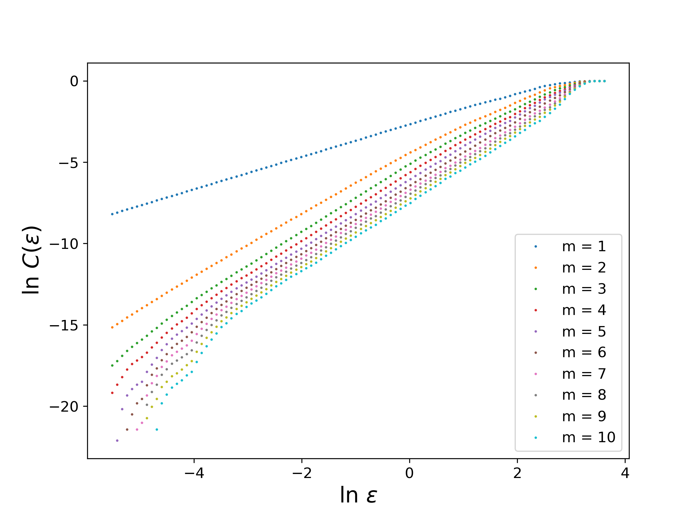
(a) Correlation sum calculations

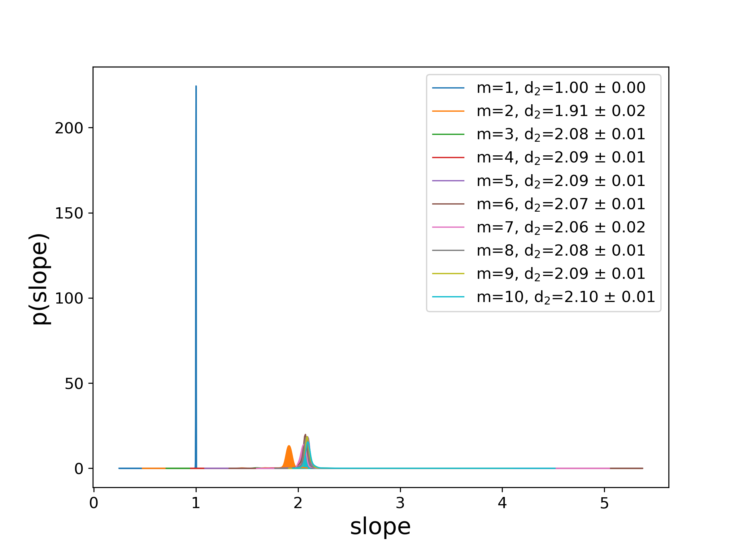
(b) Weighted slope distributions

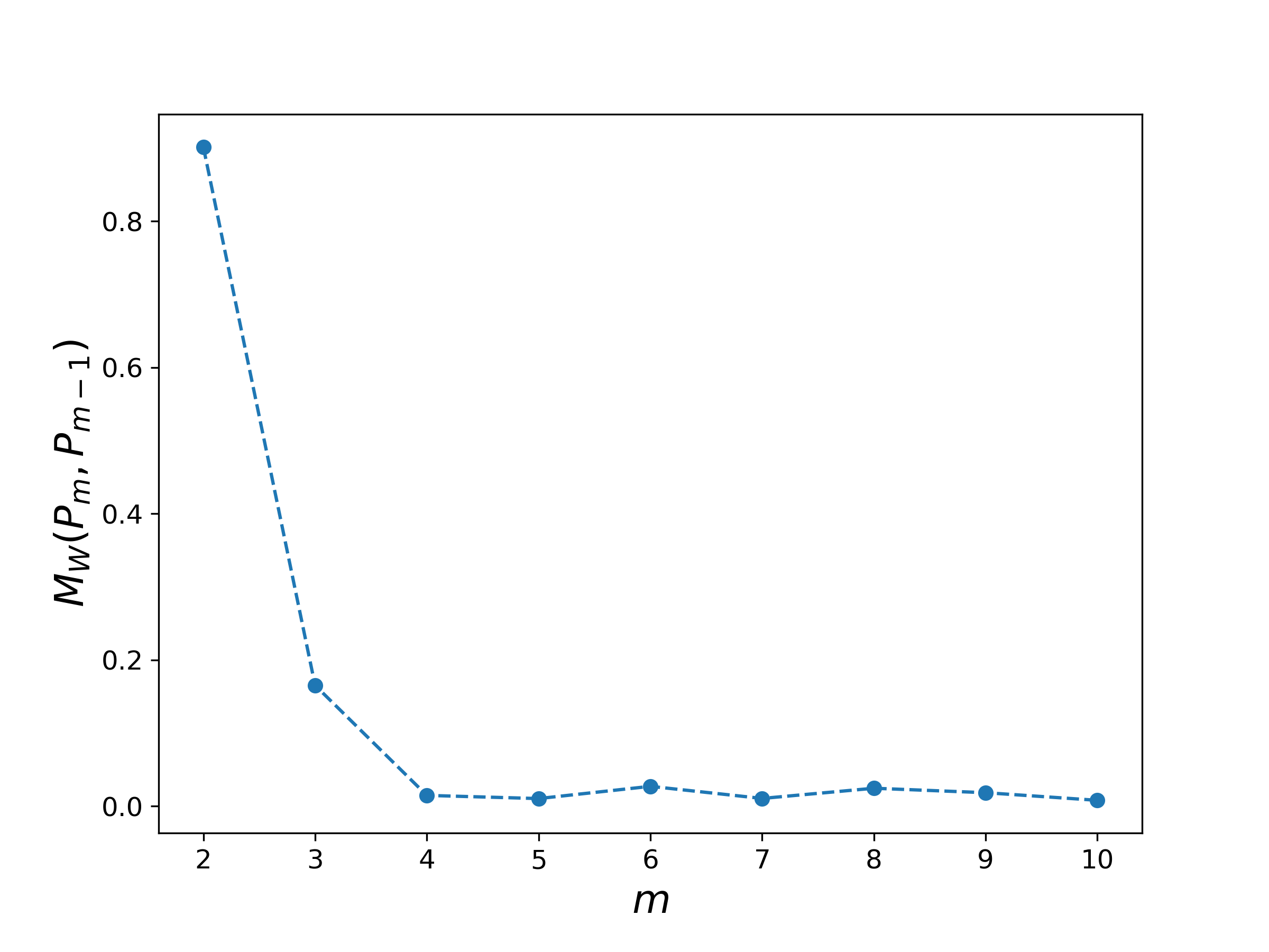
(c) Wasserstein distance

Figure 8: Correlation dimension from time-delay reconstructions of the Lorenz system for $x(t)$, $\tau=18$ and $m\in[1,10]$. Each $m$ from (a) gives a slope distribution (b), and these are pairwise compared in (c) using the Wasserstein distance.

As is well known, we can assess the convergence of $d_{2}$ by reasoning about such a sequence of curves. When $m$ is too small, the reconstructed attractor is improperly unfolded, giving an incorrect dimension, while for large enough $m$, $d_{2}$ typically converges—modulo data limitation issues—to the nominally correct value. Since our ensemble methodology automates the calculation of scaling regions, it can simplify this calculation for multiple curves. To determine the value of $m$ for which the slopes converge, one simply computes the modes of each slope distribution and looks for the $m$ value at which the positions of those modes stabilize. For Fig. 8(a), the mode for $m=1$ is, of course, $d_{2}=1$, but when $m$ reaches $3$, the distributions begin to overlap and for $3\leq m\leq 5$ the modes are $2.09\pm 0.01$, essentially the estimate from the full dynamics in §III.1.1.

To formalize this procedure, we use the Wasserstein metric $M_{W}$ to compare the two distributionsVallender (1974). Informally, this metric—called the “earth mover’s distance”—treats each distribution as a pile of soil, with the distance between the two distributions defined as the minimum “effort” required to turn one pile into another. Thus $M_{W}=0$ only when the distributions are identical. We use the python scipy.stats.wasserstein_distance package to compute this metric.

Given slope distributions $P_{m}$ and $P_{m-1}$ for successive embedding dimensions from Fig. 8(b), the distance $M_{W}(P_{m},P_{m-1})$ is shown in panel (c) of the figure. Note that $M_{W}(P_{m},P_{m-1})$ initially decreases rapidly with increasing $m$, approaching zero at $m=4$. Up to fluctuations, $M_{W}(P_{m},P_{m-1})$ remains approximately constant thereafter. Through experiments across multiple examples, we heuristically propose a threshold $M_{W}(P_{m},P_{m-1})\sim 0.1$ to estimate convergence of $d_{2}$ as $m$ grows. Such a threshold has two benefits, giving both an estimate of the embedding dimension and of $d_{2}$.

To assess the generality of these ideas, we applied the ensemble-based method to four additional scalar time series: the noisy Lorenz data of §III.1.3 with $\delta=0.1$ using $x(t)$, the pendulum trajectory of §III.1.2 using the $\omega(t)$, a shorter, $200,000$ point segment of this orbit, and finally, a trajectory from the Lorenz-96 model Lorenz (2006). In each case, we again used the curvature-based heuristic of Ref. [Deshmukh et al., 2020] to estimate $\tau$. This set of examples represents a range of problems that can arise in practice: measurements affected by noise, and a trajectory that is too short to fully cover an attractor, and a high-dimensional attractor.

System	Full Dynamics	Reconstructed
	$d_{2}$	$d_{2}$	$\tau$	$m$
Lorenz (III.1.1)	$2.09\pm 0.02$	$2.09\pm 0.01$	18	4
Noisy Lorenz ($\delta=0.1$)	$2.59\pm 0.20$	$2.27\pm 0.14$	21	7
Pendulum (III.1.2)	$2.22\pm 0.02$	$2.16\pm 0.02$	120	4
Truncated Pendulum	$2.23\pm 0.07$	$2.20\pm 0.03$	120	4
Lorenz-96	$5.63\pm 0.09$	$5.80\pm 0.07$	24	10

Table 1: Correlation dimensions calculated using the ensemble-based method with Wasserstein distance for five cases. The histograms for each of these examples are shown in Appendix C.

The results, presented in Table 1 show that $d_{2}$ for the reconstructed dynamics is close to that of the full dynamics as well as that given previously by manually fitting scaling regions Deshmukh et al. (2020). However, the embedding dimensions are often significantly smaller that those suggested by other work. For the first four examples in Table 1, for example, Ref. [Deshmukh et al., 2020] used $m=7=2d+1$, the dimension required by the Takens theorem for a three-dimensional state space Takens (1981); for the Lorenz-96 example, that paper used $m=12$, obtained from the heuristic $m>2d_{cap}$ Sauer, Yorke, and Casdagli (1991). Both $m\geq 2d+1$ and $m>2d_{cap}$ are sufficient conditions, of course. The Wasserstein test used in Table 1 shows that accurate estimates of $d_{2}$ can often be obtained with a lower embedding dimension and without prior knowledge of the original dynamics.

III.2 Lyapunov Exponent

Computing a Lyapunov exponent also often involves identification and characterization of scaling regions. Here we will use the Kantz algorithm Kantz (1994) to estimate the maximal Lyapunov exponent $\lambda_{1}$ for a reconstructed trajectories of the Lorenz and chaotic pendulum examples from §III.1.4. We embed the scalar data using a delay $\tau$ found by standard heuristics, and experiment with various embedding dimensions. The Kantz algorithm starts by finding all of the points in a ball of radius $\epsilon_{s}$ (also called the “scale”) around randomly chosen reference points on an attractor. By marching through time, the algorithm then computes the divergence between the forward image of the reference points and the forward images of the other points in the $\epsilon_{s}$ ball. The average divergence across all reference points at a given time is the stretching factor. To estimate $\lambda_{1}$, one identifies a scaling region in the log-linear plot of the stretching factor as a function of time.

Note that this procedure involves three free parameters: the embedding parameters $\tau$ and $m$ and the scale of the balls used in the algorithm. To obtain accurate results one is confronted by an onerous multivariate parameter tuning problem, and an automated approach can be extremely advantageous. If, for example, one embeds the $x$ coordinate of the Lorenz data from §III.1.1 with $m$ ranging from 2 to 9 and chooses 10 values of $\epsilon_{s}$ (e.g., on a logarithmic grid with 10 values between 0.038 and 0.381), then there will be 80 different curves, as seen in Fig. 9(a). Manually fitting scaling regions to each curve would be a demanding task.

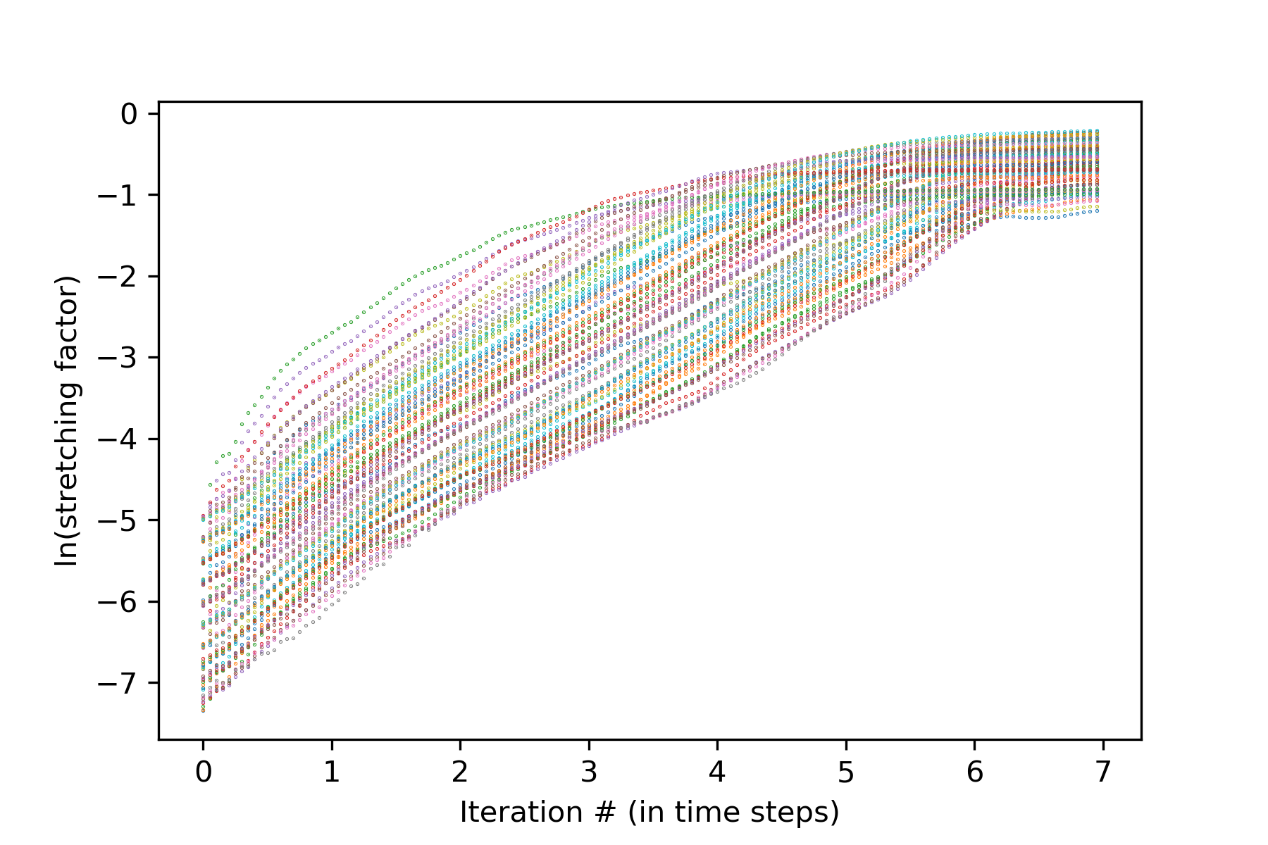
(a) Stretching factor calculations (Lorenz)

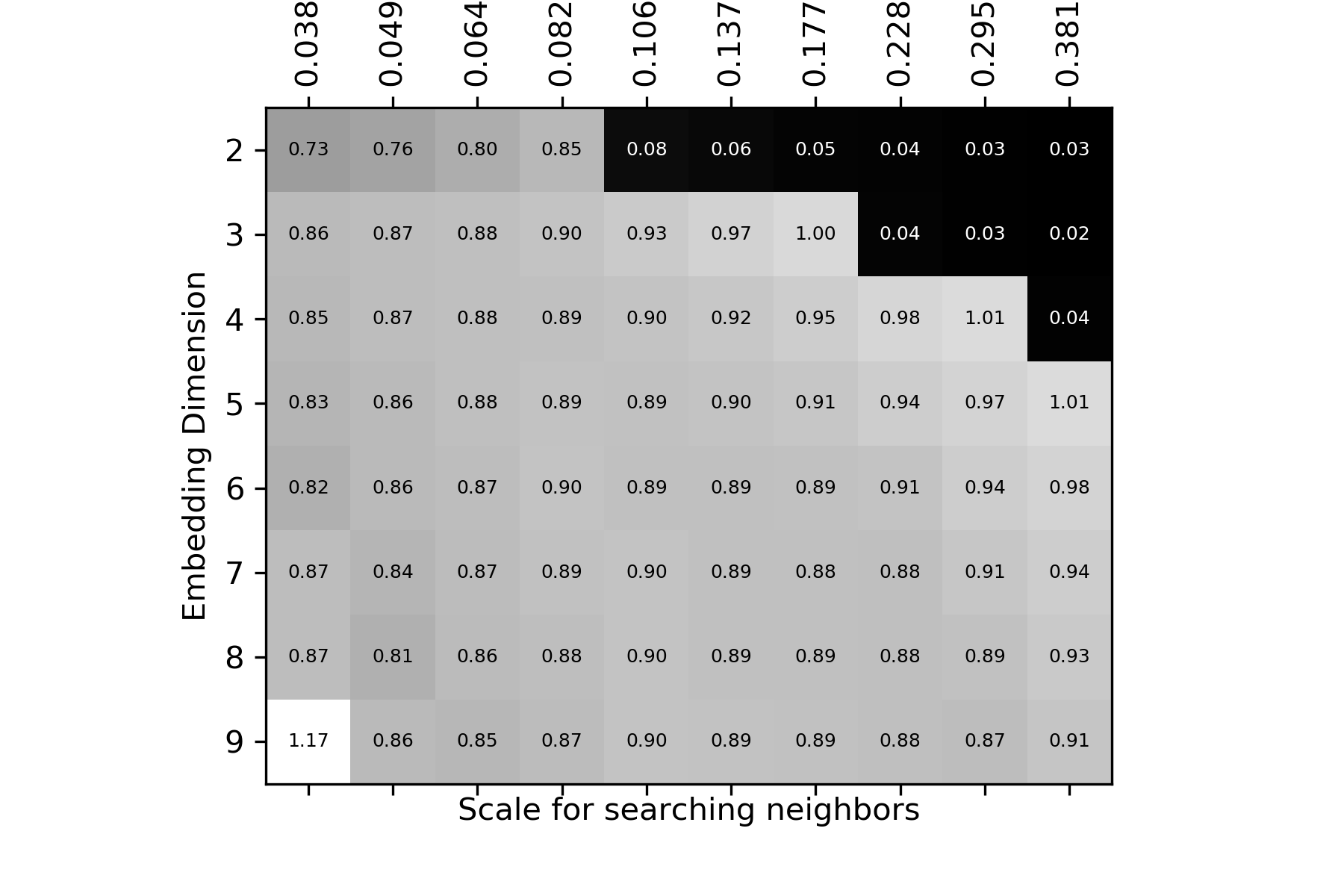
(b) $\lambda_{1}$ estimate (Lorenz)

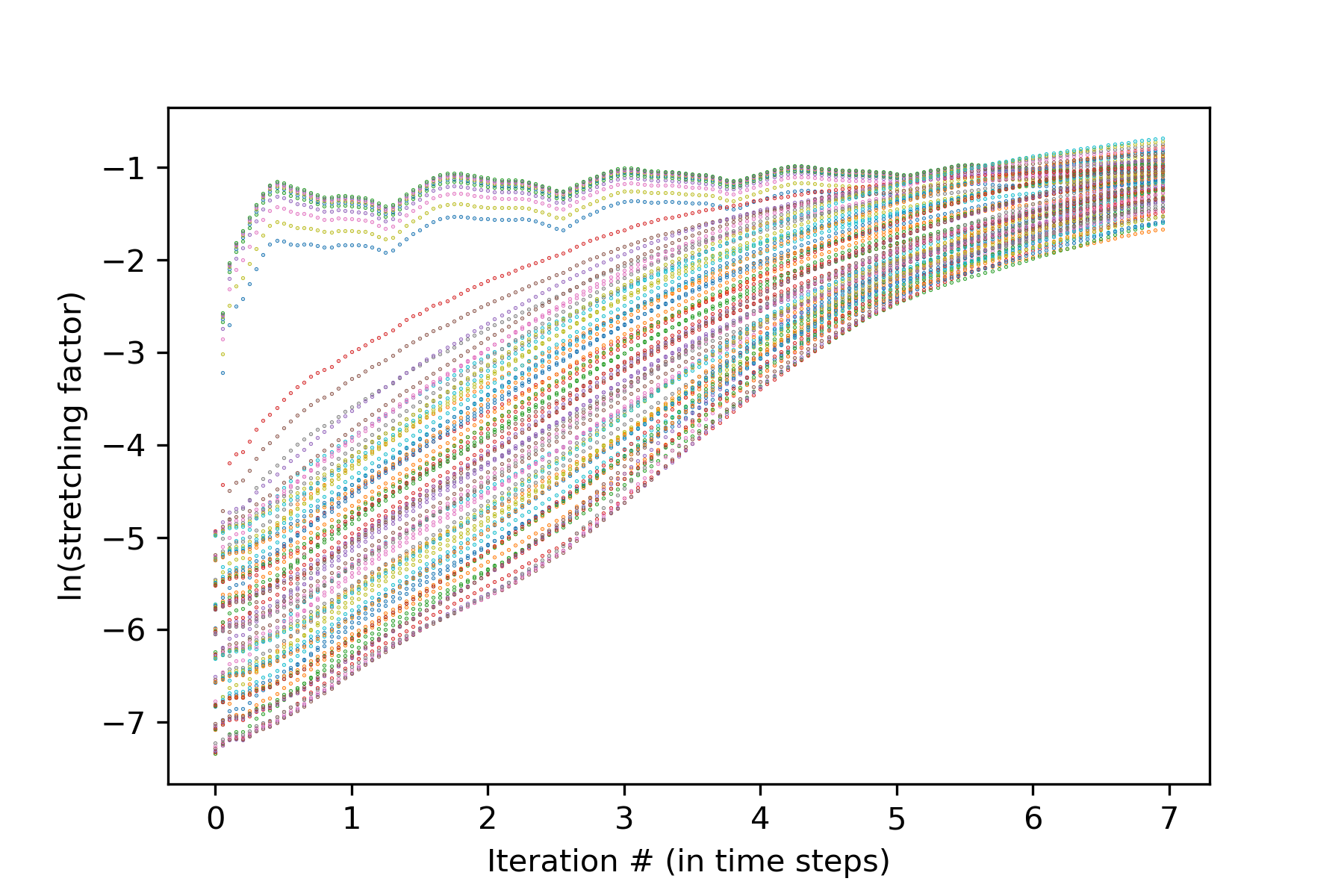
(c) Stretching factor calculations (pendulum)

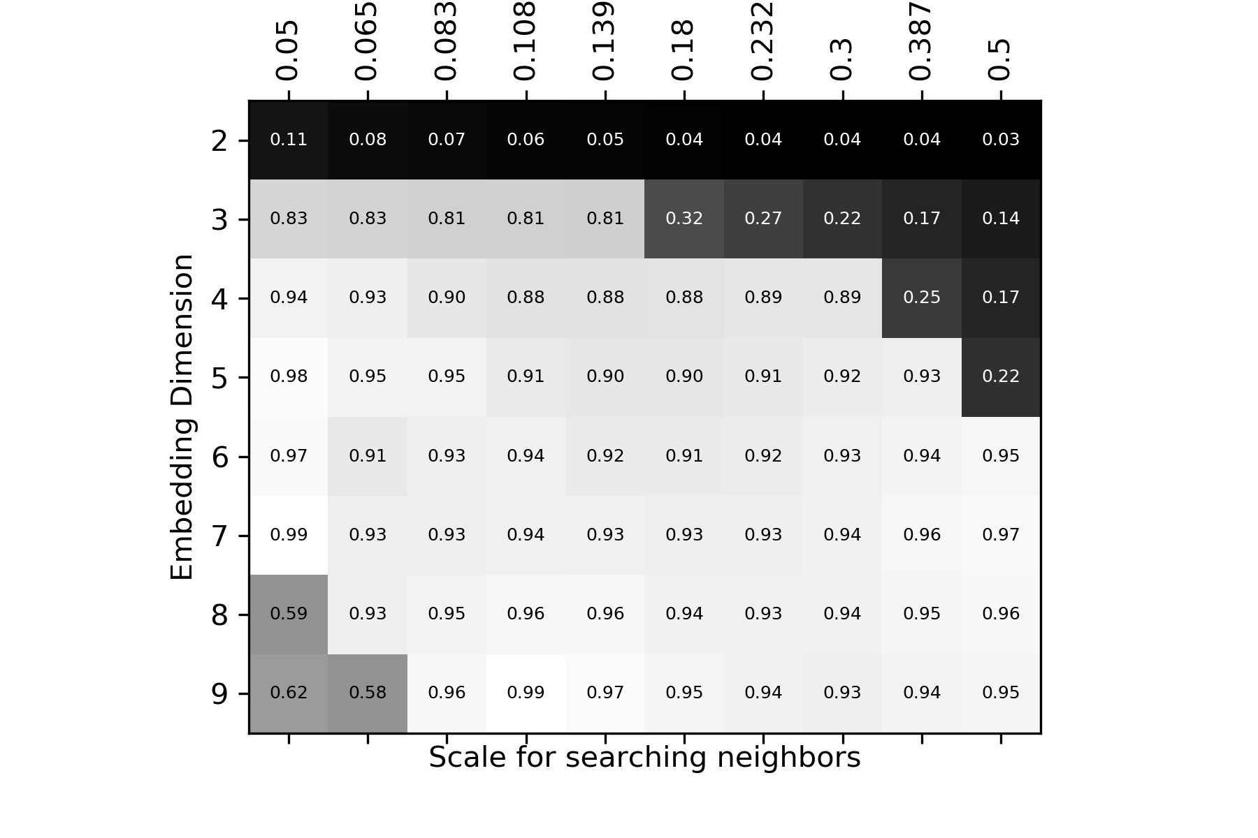
(d) $\lambda_{1}$ estimate (pendulum)

Figure 9: Estimating the largest Lyapunov exponent $\lambda_{1}$ of the Lorenz and driven, damped pendulum examples. Panels (a) and (c) show stretching-factor calculations for the eight embedding dimensions $m$ and ten search scales $\epsilon_{s}$. The estimated exponents for all the dimensions and scales are shown in grid form in panels (b) and (d). The gray scale in each grid cell represents the magnitude of the exponent.

The ensemble method gives the automated results shown in panel (b) of the figure.

Each row of this 2D grid corresponds to fixed $m$ and each column to fixed $\epsilon_{s}$. The estimated $\lambda_{1}$—the location of the mode in the slope PDF—is the value shown in the cell. To help detect convergence, each cell is shaded according to the corresponding $\lambda_{1}$ value. Note that the majority of the configurations (48 out of 80, colored in intermediate gray) give an estimate of $\lambda_{1}=0.89\pm 0.02$, which is consistent with the known value Grigorenko and Grigorenko (2003).

The pattern in the grid make sense. The cells in its center correspond to midrange combinations of the free parameters: $m\in[5,9]$ and $\epsilon_{s}\in[0.064,0.177]$. Values outside these ranges create well-known issues for the Kantz algorithm in the context of finite data. If $\epsilon_{s}$ is too small, the ball will not contain enough trajectory points to allow the algorithm to effectively track the divergence; if $\epsilon_{s}$ is too large, the ball will straddle a large portion of the attractor, thereby conflating state-space deformation with divergence. For $m$ too small, the attractor is insufficiently unfolded, so the values in the top few rows of the grid are suspect. In the upper right corner, these two effects combine: the attractor is both insufficiently unfolded and also spanned by the $\epsilon_{s}$ ball. Also, the zero slope portion on the right ends of the stretching factor curves becomes dominant (since since the $\epsilon_{s}$ ball reaches the edge of a flattened attractor more quickly) thus causing the ensemble-based algorithm to return a slope close to zero. Finally, we see a slightly higher estimate of $\lambda_{1}=1.17$ for $m=9$ and $\epsilon_{s}=0.038$. On close inspection of the stretching factor plot for this configuration, we see significant oscillations distorting most of the curve. A relatively straighter part of these oscillations is chosen by the algorithm as a scaling region, leading to that specific estimate. Seeing how visually distorted this curve is from the curves generated for other parameter combinations, it is clear that this parameter combination should be avoided when computing the $\lambda_{1}$ estimate.

The process is repeated for the driven damped pendulum example in Fig. 9(c,d). Here, we use a slightly different trajectory than in section III.1.2: $500,000$ points (after removing a transient of $50,000$ points) with a time step of $0.01$. For this trajectory, the heuristic of Ref. [Deshmukh et al., 2020] suggests an embedding delay of $\tau=21$. From the grid, we observe similar patterns as in the Lorenz example: 46 out of 80 combinations give $\lambda=0.93\pm 0.04$ (for $m\in[4,9]$ and $\epsilon_{s}\in[0.083,0.3]$). We observe significantly lower estimates when the embedding dimension is low and $\epsilon_{s}$ is high. Additionally, an anomalous behavior similar to the Lorenz example is observed for higher embedding dimensions ($m\in[8,9]$) and smaller scales ($\epsilon_{s}\in[0.05,0.065]$). Here, we see lower estimates ($0.60\pm 0.02$) for these parameter configurations. The underlying cause in this case is low frequency oscillations in the stretching factor plots, with a relatively straight region towards the right end of the plots where they start to flatten. As for the Lorenz example, these parameter combinations should be avoided for the $\lambda_{1}$ estimate.

The ensemble approach allows us to easily automate computation of scaling regions for various values of the hyperparameters, thus sparing significant manual labor. Moreover, the grid visualization allows us to find the “sweet spot” in the free-parameter space. While this is only a relatively crude convergence criterion, one could instead use a more rigorous test such as the Wasserstein distance of § III.1.4.

IV Conclusions

The technique described above is intended to formalize a subjective task that arises in the calculation of dynamical invariants, the identification and characterization of a scaling region: an interval in which one quantity grows linearly with some other quantity. By manipulating the axes, one can extend this to detect exponential or power-law relationships: e.g., using log-log plots for fractal dimensions and log-linear plots for Lyapunov exponents, as shown in Sections III.1 and III.2. Moreover, linearity is not a limitation in the applicability of our approach: it can be used to identify regions in a dataset with any hypothesized functional relationship (e.g. higher order polynomial, logarthmic, exponential, etc.). One would simply compute the least squares fit over the data using the hypothesized function instead.

A strength of our method is that the scaling region is chosen automatically as the optimal family of intervals over which the fits have similar slopes with small errors. To do this, we create an ensemble of fits over different intervals to build PDFs, to identify the boundaries and slopes of any scaling regions, and to obtain error estimates. When the scaling region is clear, our ensemble-based approach computes a slope similar to that which would be manually determined. We showed that a convergence test on the slope distributions helps choose the delay reconstruction dimension. This is a challenging task: even though there are powerful theoretical guidelines, the information needed to apply them is not known in advance from a given scalar time-series.

This kind of objective, formalized method is useful not only because it reveals scaling regions that may not be visible, but also because it provides confidence in its existence by providing error estimates. Moreover, since computing a dynamical invariant, such as the Lyapunov exponent, can involve finding scaling regions in many curves, an automated method provides a clear advantage over hand selection of scaling regions. Our method could be potentially useful in areas outside dynamical systems as well: e.g., estimating the scaling exponent for data drawn from a power-law distribution. This is an active area of research Alstott, Bullmore, and Plenz (2014); Clauset, Shalizi, and Newman (2009). Standard techniques involve inferring which power-law distribution (if any) the data is most likely drawn from, and—if so—which exponent is most likely. Our method could potentially help narrow down the range of exponents to begin such a search.

There are a number of interesting avenues for further work, beginning with how to further refine the confidence intervals for slope estimates. We have used the standard deviation of the slopes within the $FWHM$ around the mode of the distribution. Alternatively, one could use the average of the least squares fit error across all the samples within the $FWHM$ as the confidence interval. Another possibility is to first extract a single scaling region (by determining the modes for the left- and right-hand side markers) and computing the error statistics over all the sub-intervals that are sampled from this scaling region (e.g., standard deviation of the slopes or the average of the fit errors). We used the Wasserstein distance to assess the convergence of a sequence of slope distributions to help choose an embedding dimension. This may be too strict since it requires that the entire distributions are close. One could instead target the positions of the modes, quantifying closeness using some relevant summary statistic like their confidence interval. Of course, in cases of multimodal distributions, the Wasserstein distance test is more appropriate since we cannot choose a single mode for computing the intervals.

Data Availability

The data that supports the findings of this study are available within the article.

Appendix A Algorithm

The pseudocode for the proposed ensemble-based approach is described in Algorithm 1. There are four important choices in this algorithm. The first is the parameter $n$, the minimum spacing between the left-hand and right-hand side markers $LHS$ and $RHS$. This choice limits what is deemed to be a “significant interval” for a scaling region. We set $n=10$ in this paper, which we chose using a persistence analysis, that is varying $n$ and seeing if the results change. One could argue for increasing $n$ for a data set with more points; however, pathologies in the data set could violate that argument. The second is the choice of a kernel density estimator (KDE) for the histograms. We used the Gaussian KDE with the python implementation scipy.stats.gaussian_kdeVirtanen et al. (2020) of Scott’s methodScott (1979) to automatically select the kernel bandwidth. Alternatively, one might choose other bandwidth selection methods, such as Silverman’s methodSilverman (1986), or simply manually specify the bandwidth. Scott’s method, which is the default method used by the package, worked well for all our examples.

Algorithm 1 Ensemble approach for estimating the slope of scaling regions

1:Assume a plot $(x[0:length-1],y[0:length-1])$ that potentially contains a scaling region.

2:Initialize empty arrays $slopes$, $lengths$, $errors$, $x_{l}$ and $x_{r}$.

3:for $lhs=0,1,2,\ldots,length-1$ do

4:     for $rhs=0,1,2,\ldots,length-1$ do

5:         if $rhs-lhs>n$ then

6:              Fit a line using least squares to data $x[lhs:rhs],y[lhs:rhs]$.

7:              Obtain an estimate for slope $m$ and intercept $c$.

8:              Compute the least squares fit length and fitting error,

$$\text{fit length}=\sqrt{1+m^{2}}\left|x[rhs]-x[lhs]\right|,$$ (5)

$$\text{fit error}=\sqrt{\frac{\sum_{i=lhs}^{rhs}(y[i]-mx[i]-c)^{2}}{rhs-lhs}}.$$ (6)

9:              Append the slope, length and error to the arrays $slopes$, $lengths$ and $errors$, respectively.

10:              Append $x[lhs]$ and $x[rhs]$ to endpoint arrays $x_{l}$ and $x_{r}$, respectively.               

11:Generate a histogram $H$ from the $slopes$ array, weighting each point by

$$\text{weight[i]}\propto\frac{\text{(fit length[i])}^{p}}{\text{(fit error[i])}^{q}},$$ (7)

for suitable powers $p$ and $q$.

12:Using a kernel density estimator, generate a probability distribution function $P$, from $H$ (see e.g. Fig. 1(b)).

13:Compute the mode(s) of $P$ and the error estimates as described in Sec. II.

14:Generate histogram $H_{l}$ and $H_{r}$ for $x_{l}$ and $x_{r}$ from Step 10, weighting the frequency with (7). Generate PDFs and evaluate them on the $x$ interval, as in Step 12, to generate distributions $P_{l}$ and $P_{r}$ (see e.g. Fig. 1(c)).

The two other important parameters are the powers $p$ and $q$ used for the weights of the length and the error of the fit in (7). We explored ranges for these parameters, constraining $p$ and $q$ to nonnegative integers, and determined suitable values that worked well for all of the examples considered here. Some interesting patterns emerged in these explorations. Firstly, we found that $p>0$ helps to reduce the error estimate for the slope $\sigma$ and improve $p_{FWHM}$. Note that $p>0$ penalizes the shorter fits near the edges of the $FWHM$, suppressing their influence on the histogram. The $FWHM$ therefore narrows, in turn reducing the error estimate $\sigma$. Secondly, setting $p\leq q$ was found to be advantageous in all cases, ensuring that the algorithm does not prioritize unnecessarily longer fits of poor quality. Enforcing these two conditions, we experimented with a few choices for $p$ and $q$ in the context of the first example of Fig. 1, and found that lower $p,q$ values generally work better. Higher powers tend to magnify effects of small errors and small lengths, making the algorithm very conservative in terms of what constitutes a good fit. With this in mind, we settled on $p=1$ and $q=2$ for the correlation dimension estimation, finding that those values generalized well across all the examples. For the Lyapunov exponent examples, on the other hand, we found that $p=1$ and $q=1$ does better, generating tighter confidence interval bounds around the estimate across the various parameter combinations.

This algorithm always uses the full data set to compute the ensemble but note that it does not require even spacing of the data. Given a much larger data set, it might make sense to downsample to speed up the algorithm. In its current implementation, the run-time complexity of the algorithm is $O(N^{2})$, for a relationship curve with $N$ points. In the future, it might be useful to develop faster algorithms for sampling and generating the slope distributions.

Appendix B Effects of noise on the Lorenz attractor

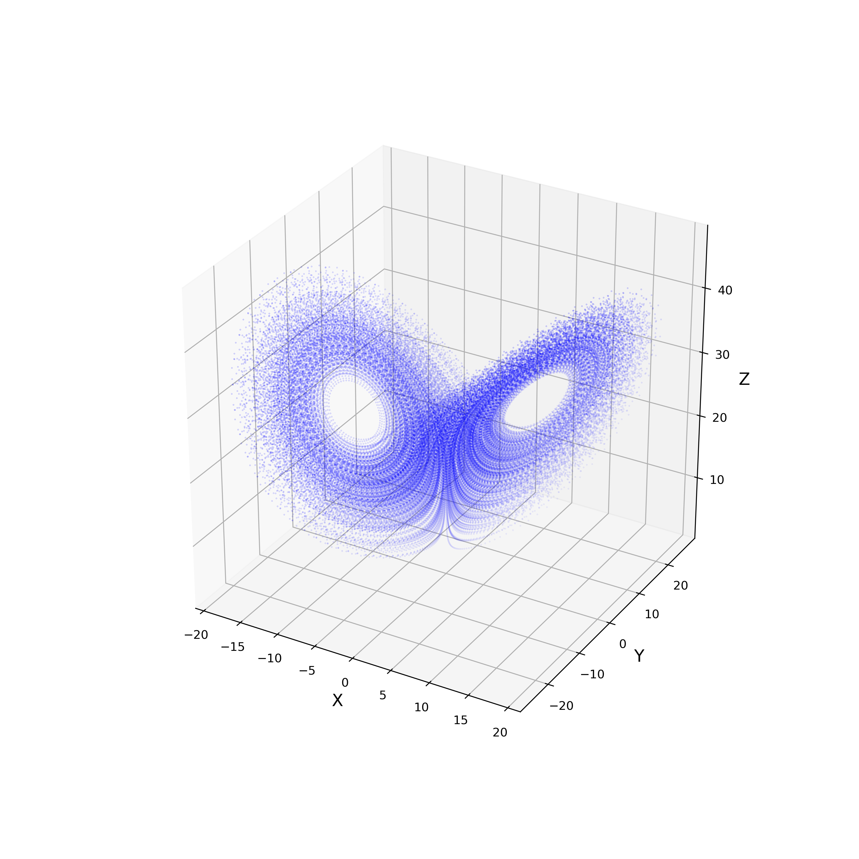
(a) Noiseless Lorenz trajectory

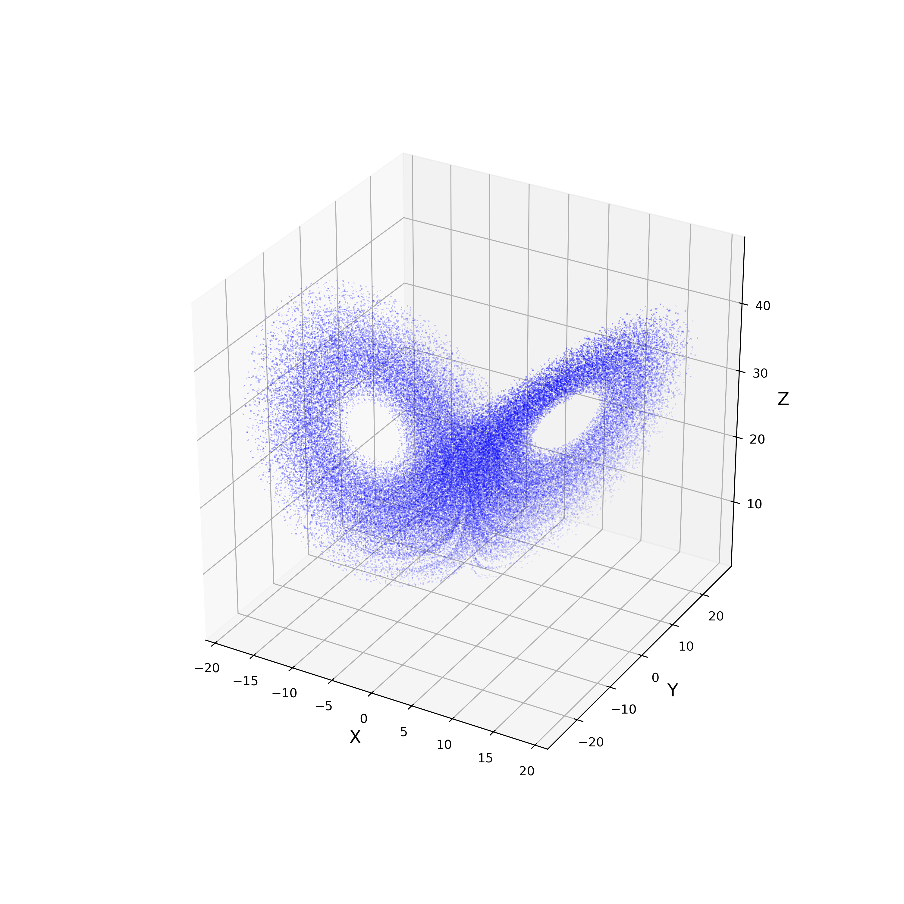
(b) Noisy Lorenz trajectory ($\delta=0.01$)

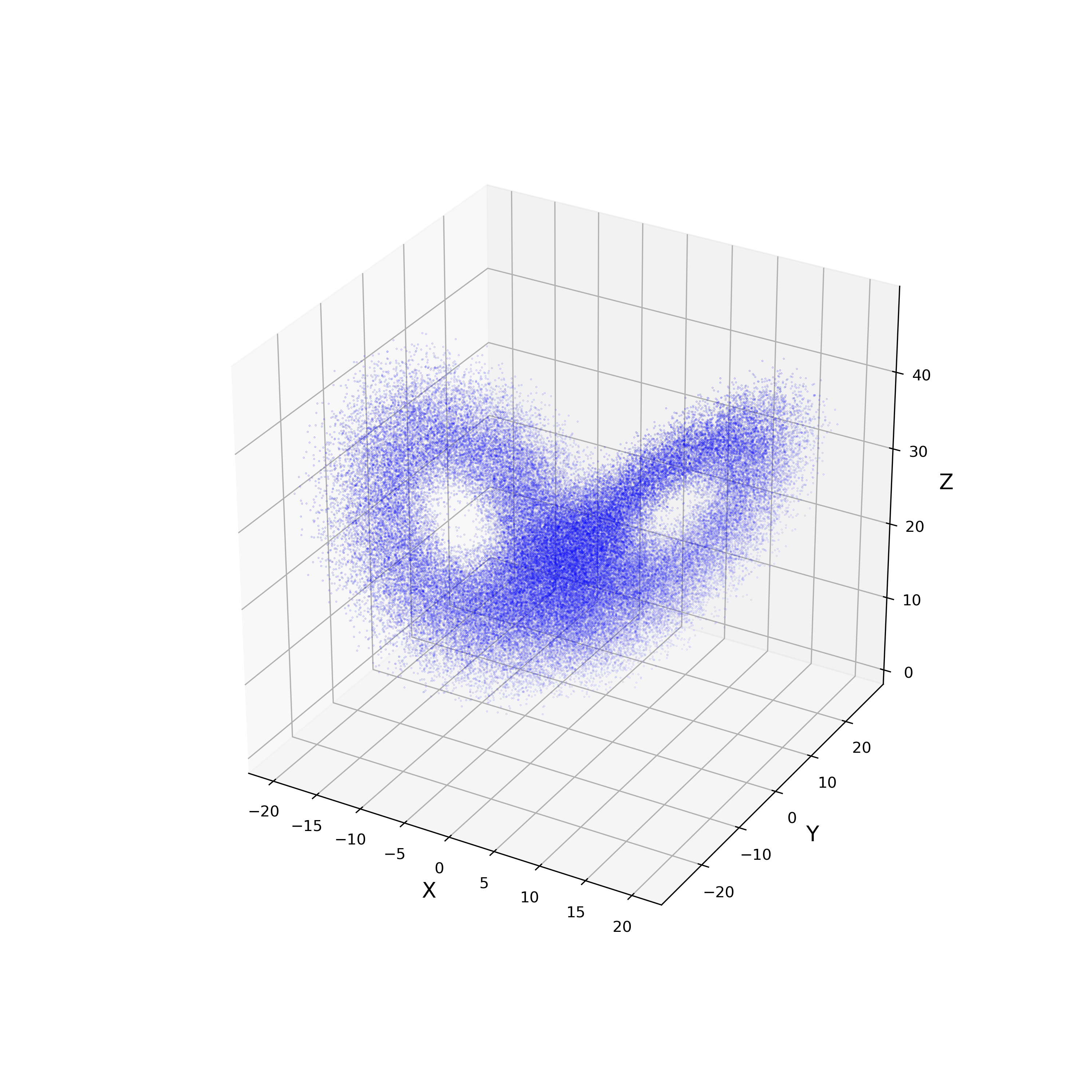
(c) Noisy Lorenz trajectory ($\delta=0.1$)

Figure 10: Effect of noise on the Lorenz attractor with different magnitudes of noise level $\delta$.

Fig. 10 shows the effect of noise on the Lorenz attractor, the resulting noisy attractor used in Section III.1.3. As we increase the noise level (as a fraction of the attractor radius) $\delta$ from 0.0 to 0.1, we see the dynamics of the attractor getting progressively distorted. As discussed in Section III.1.3, the effects of this distortion on the correlation dimension plots and hence the slope distributions are clearly visible.

Appendix C Time Series Reconstruction: Additional Plots

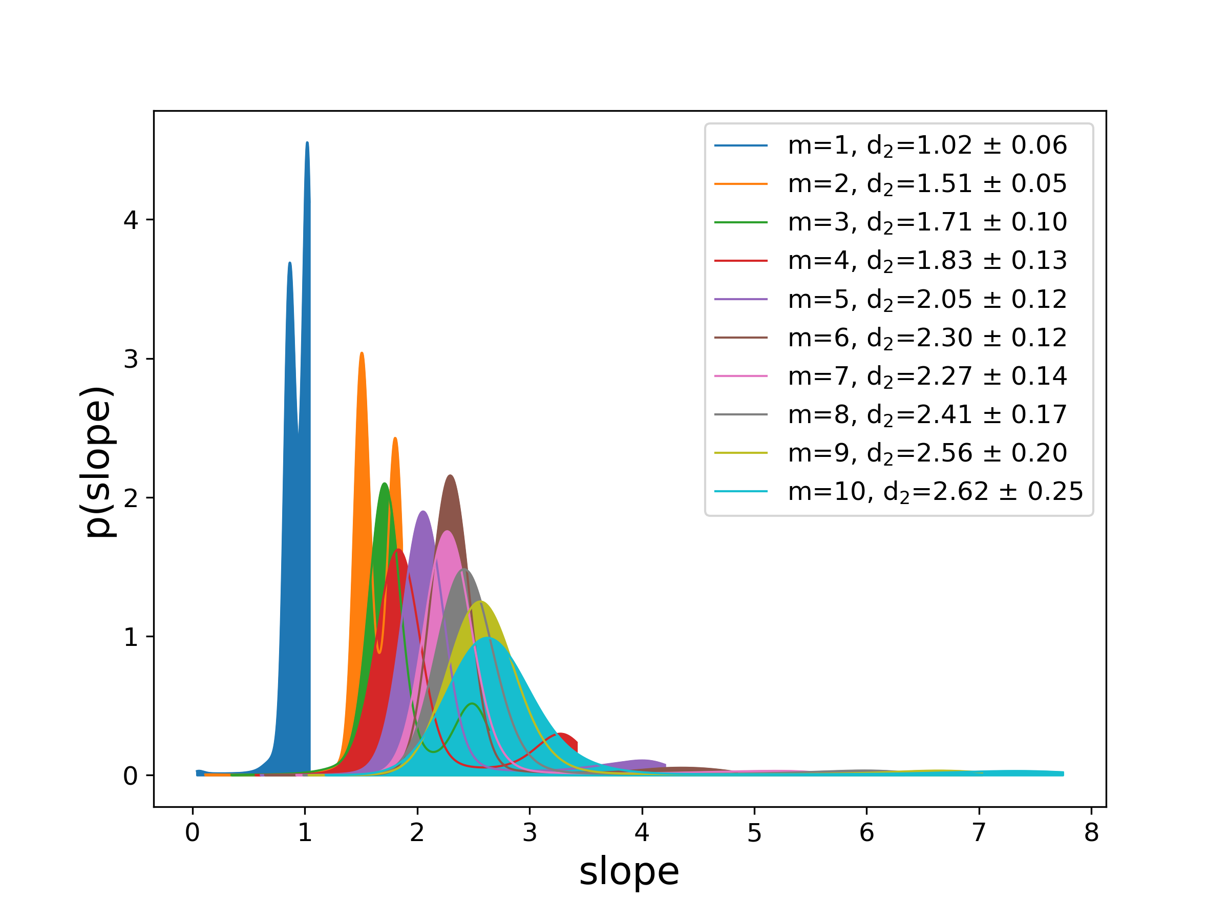
(a) Weighted slope distributions ($\tau=21$)

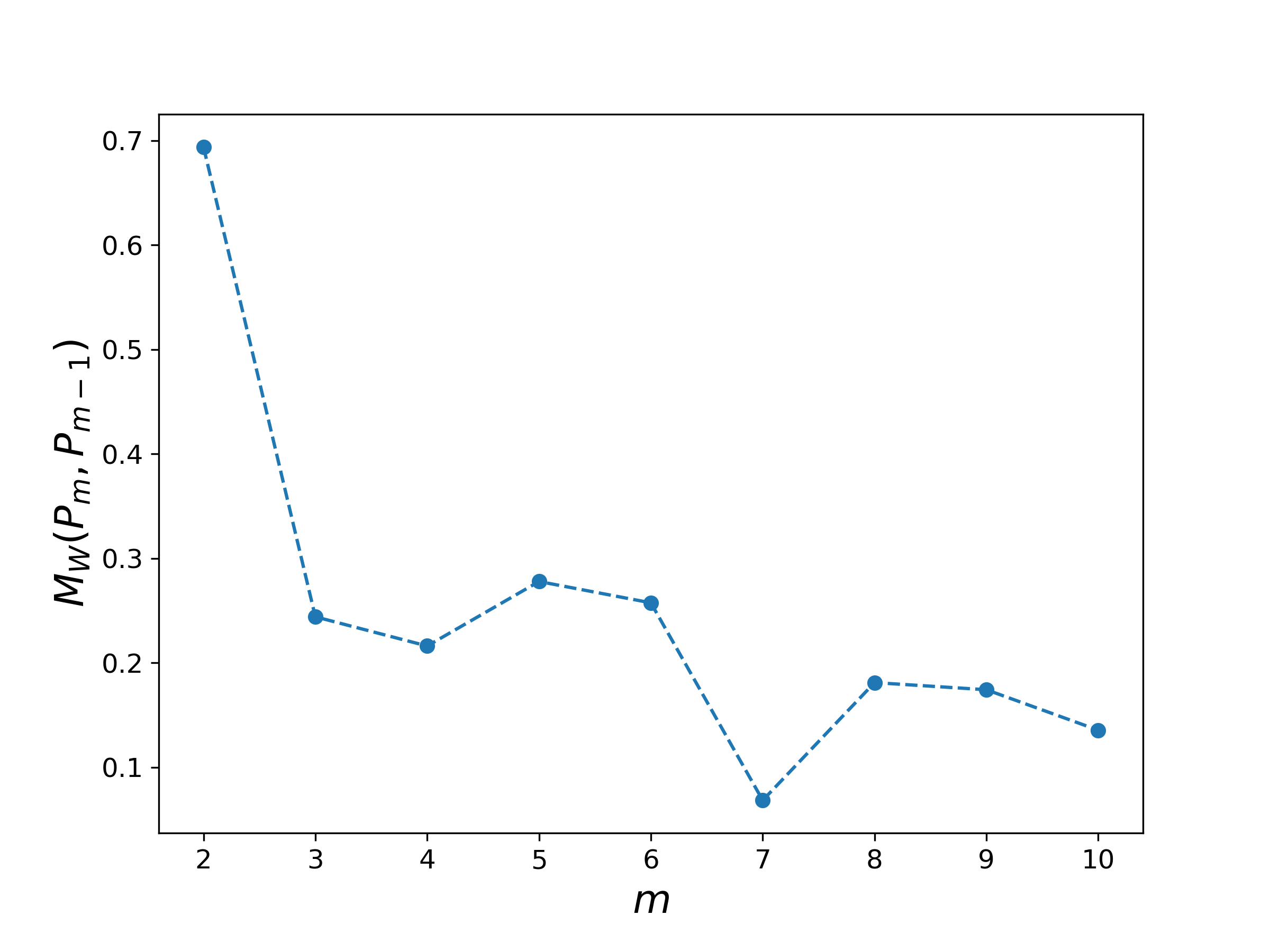
(b) Wasserstein distance ($\tau=21$)

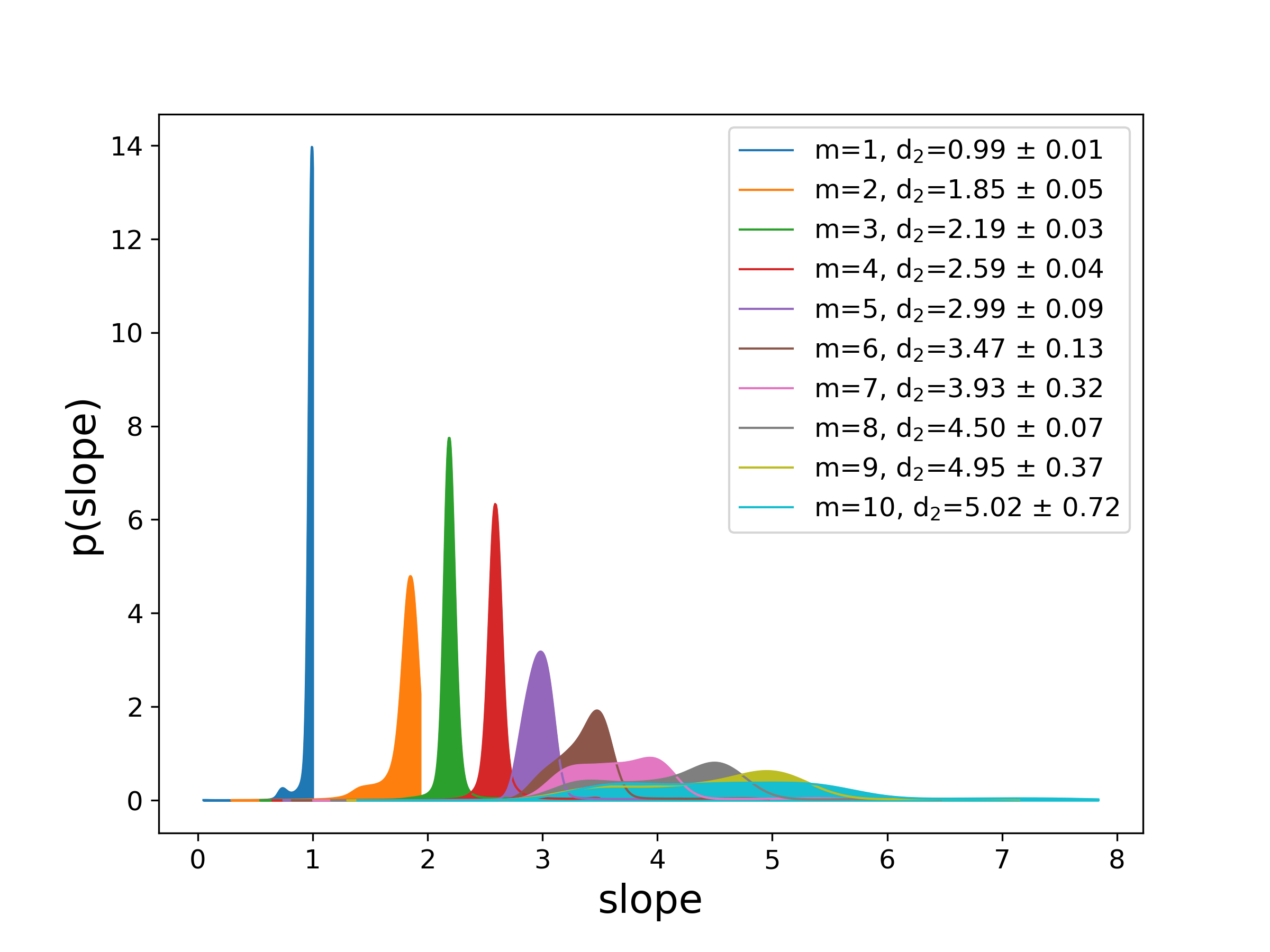
(c) Weighted slope distributions ($\tau=60$)

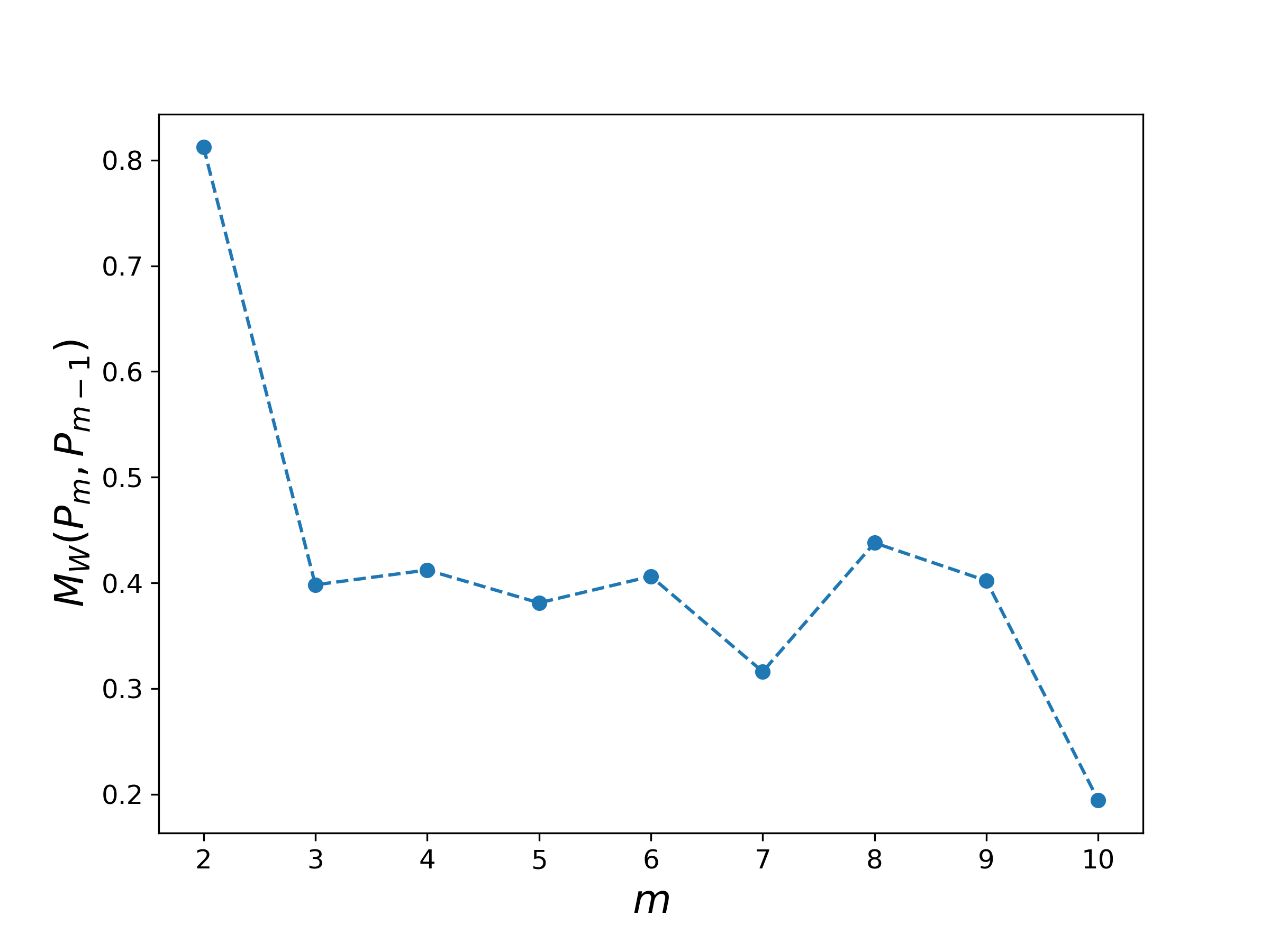
(d) Wasserstein distance ($\tau=60$)

Figure 11: Estimating the correlation dimension for the reconstructed noisy Lorenz example using two different estimates of $\tau$. The top row shows the slope distributions and the Wasserstein distance profiles for a value of $\tau=21$, estimated using the heuristic of Ref. [Deshmukh et al., 2020], while the bottom row presents the same plots for $\tau=60$, the estimate produced using the method of average mutual information Fraser and Swinney (1986).

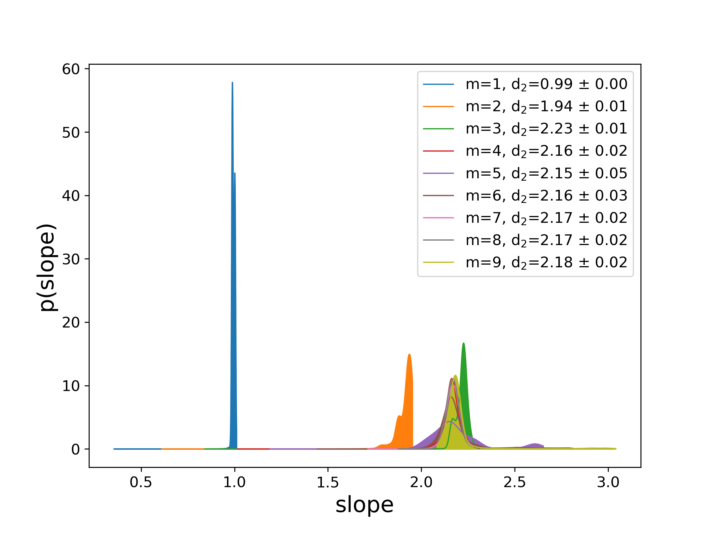
(a) Weighted slope distributions

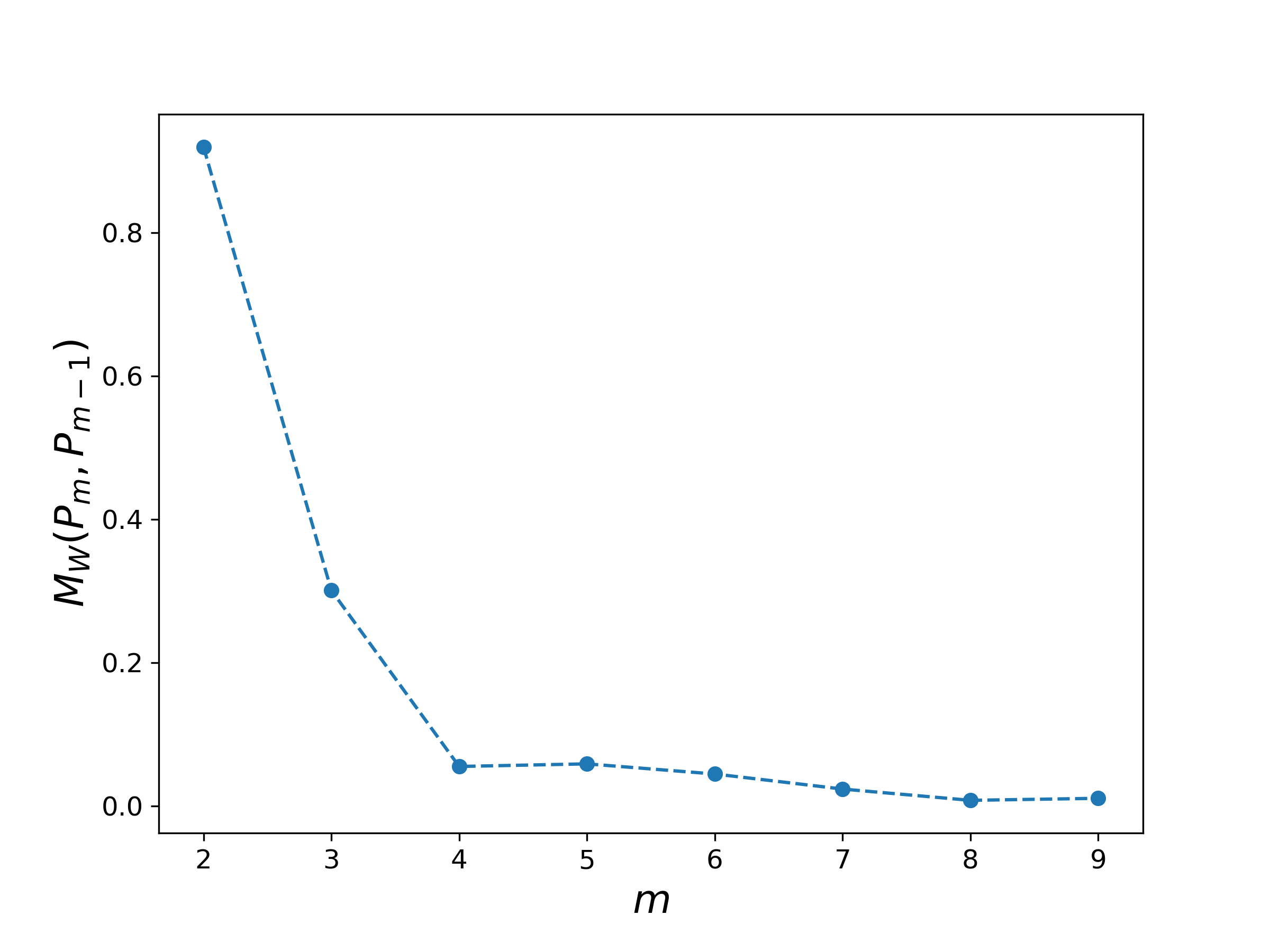
(b) Wasserstein distance

Figure 12: Estimating the correlation dimension for the reconstructed pendulum example (1M points) using a time delay estimate of $\tau=120$.

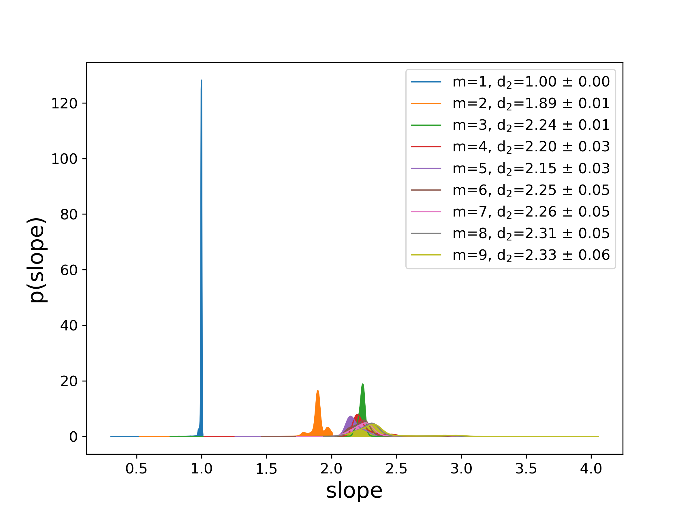
(a) Weighted slope distributions

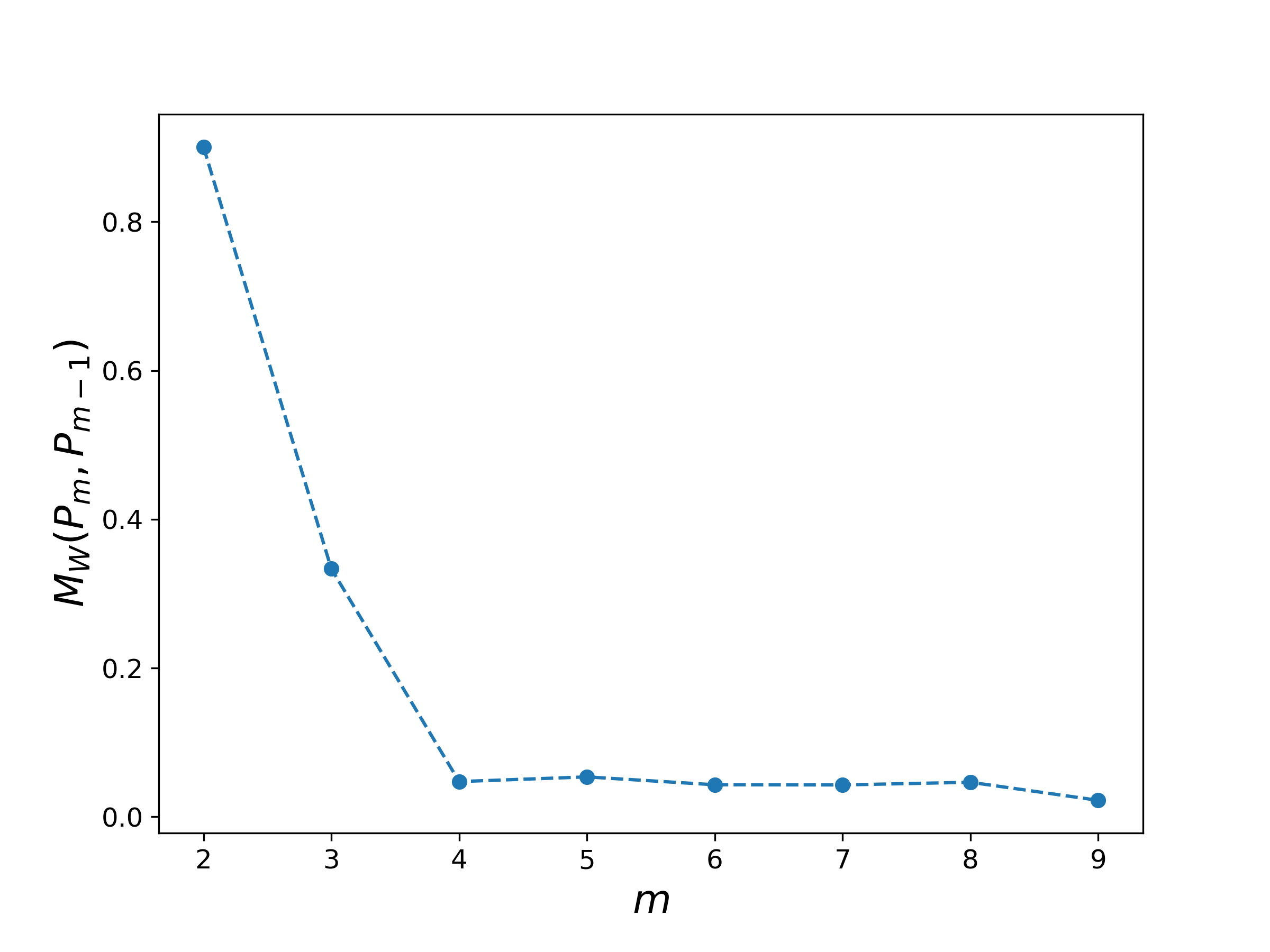
(b) Wasserstein distance

Figure 13: Estimating the correlation dimension for the reconstructed truncated pendulum example (200,000 points) using a time delay estimate of $\tau=120$.

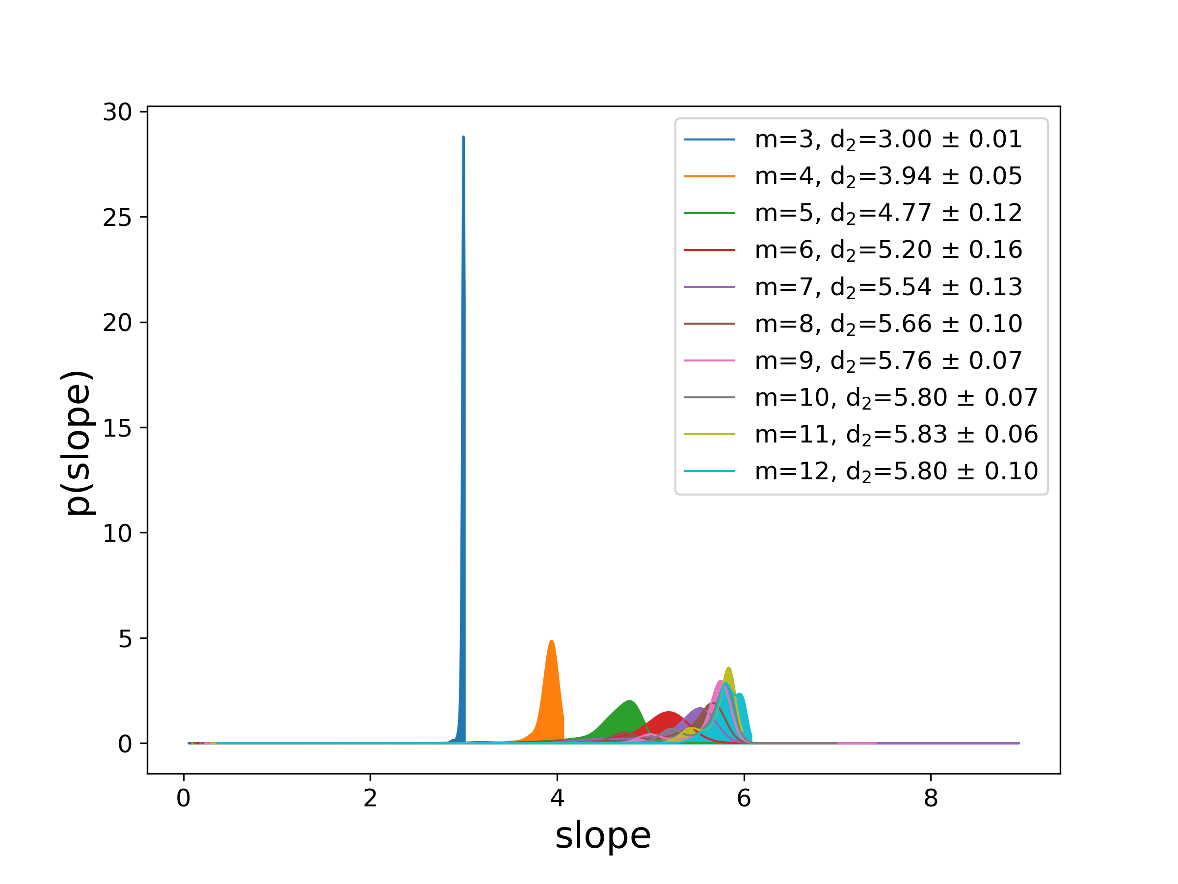
(a) Weighted slope distributions ($\tau=24$)

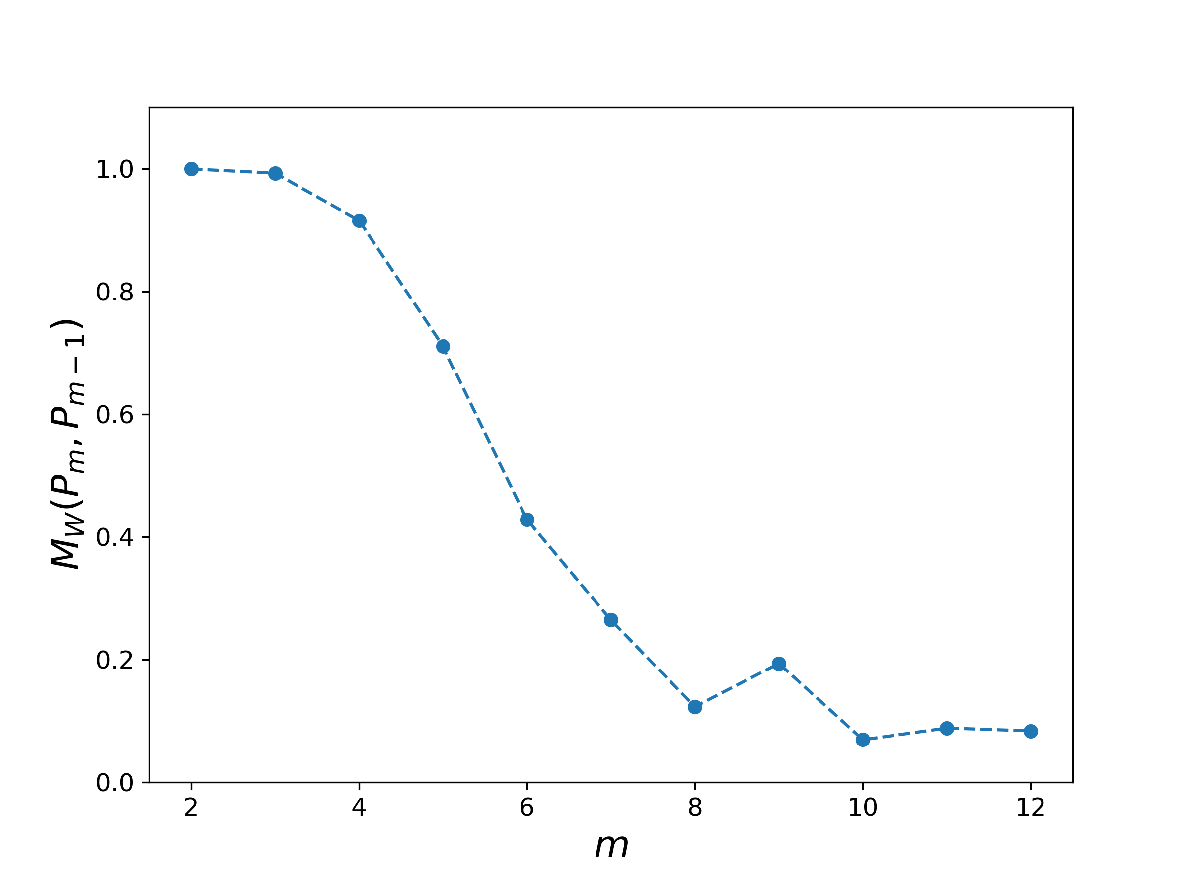
(b) Wasserstein distance ($\tau=24$)

Figure 14: Estimating the correlation dimension for the reconstructed Lorenz-96 example using a time delay estimate of $\tau=24$.

Here we present figures to support the results of Table 1. For the noisy Lorenz data, Fig. 11 shows the slope distributions and Wasserstein distance between slope distributions of consecutive embedding dimensions, $M_{W}(P_{m},P_{m-1})$. Panels (a) and (b) use $\tau=21$ as in Table 1. Note that $M_{W}(P_{m},P_{m-1})$ converges more slowly for the noisy data than it did for the deterministic case in Fig. 8. The distance $M_{W}(P_{m},P_{m-1})<0.1$ at $m=7$, giving $d_{2}=2.27\pm 0.14$.

Figures 11(c) and (d) show the reconstruction results for $\tau=60$, the embedding delay given by the average mutual information (AMI) method. Here $M_{W}(P_{m},P_{m-1})$ does not reach $0.1$ for $m\leq 10$. The implication is that the embedding dimension should be larger than $10$, contrary to the sufficient theoretical requirement of $m=7$. Indeed, panel (c) shows that the mode grows monotonically with $m$, reaching values much higher than the expected $d_{2}=2.59$ for the full dynamics.

Figures 12 and 13 show the results for the the pendulum trajectories of length $10^{6}$ and $2(10)^{5}$, respectively, generated using a delay of $\tau=120$. In both cases, the Wasserstein distance threshold is reached at $m=4$, resulting in the values in Table  1.

Finally, Fig. 14 shows the delay reconstruction of the Lorenz-96 trajectory using $\tau=24$. Convergence occurs at $m=10$, giving $d_{2}=5.80\pm 0.07$.

References

- Kantz and Schreiber (1997) H. Kantz and T. Schreiber, Nonlinear Time Series Analysis (Cambridge University Press, Cambridge, 1997).
- Bradley and Kantz (2015) E. Bradley and H. Kantz, Chaos 25, 097610 (2015).
- Ji, Zhu, and Jiang (2011) C. Ji, H. Zhu, and W. Jiang, Chinese Science Bulletin 56, 925 (2011).
- Chen, Liu, and Zhou (2019) Z. Chen, Y. Liu, and P. Zhou, Fractals 27, 1950011 (2019).
- Clauset, Shalizi, and Newman (2009) A. Clauset, C. Shalizi, and M. Newman, SIAM Review 51, 661 (2009).
- Zhou and Wang (2018) S. Zhou and X. Wang, Chaos: An Interdisciplinary Journal of Nonlinear Science 28, 123118 (2018).
- Rosenstein, Collins, and De Luca (1993) M. Rosenstein, J. Collins, and C. J. De Luca, Physica D: Nonlinear Phenomena 65, 117 (1993).
- Yongfeng et al. (2012) Y. Yongfeng, W. Minjuan, G. Zhe, W. Yafeng, and R. Xingmin, Vibration, Testing and Diagnosis 32, 371 (2012).
- Shuang et al. (2016) Z. Shuang, F. Yong, W. Wenyuan, and W. Weihua, Acta Phys 65, 020502 (2016).
- Weik (2001) M. H. Weik, “full-width at half-maximum,” in Computer Science and Communications Dictionary (Springer US, Boston, MA, 2001) pp. 661–661.
- Peitgen, Juergens, and Saupe (1992) H. Peitgen, H. Juergens, and D. Saupe, Chaos and Fractals (Spinger-Verlag, New York, 1992).
- Grassberger and Procaccia (2004) P. Grassberger and I. Procaccia, in The Theory of Chaotic Attractors (Springer, 2004) pp. 170–189.
- Grassberger and Procaccia (1983) P. Grassberger and I. Procaccia, Physical Review Letters 50, 346 (1983).
- Grassberger and Procaccia (1983) P. Grassberger and I. Procaccia, Physica D 9, 189 (1983).
- Lorenz (1963) E. Lorenz, J. Atmos. Sci. 20, 130 (1963).
- Viswanath (2004) D. Viswanath, Physica D 190, 115 (2004).
- Martínez, Domínguez-Tenreiro, and Roy (1993) V. Martínez, R. Domínguez-Tenreiro, and L. Roy, Phys. Rev. E 4, 735 (1993).
- Deshmukh et al. (2020) V. Deshmukh, E. Bradley, J. Garland, and J. D. Meiss, Chaos: An Interdisciplinary Journal of Nonlinear Science 30, 063143 (2020).
- Takens (1981) F. Takens, in Dynamical systems and turbulence (Springer, Berlin, 1981) pp. 366–381.
- Packard et al. (1980) N. Packard, J. P. Crutchfield, J. Farmer, and R. Shaw, Phys. Rev. Lett. 45, 712 (1980).
- Whitney (1936) H. Whitney, Ann. Math. 37, 645 (1936).
- Sauer, Yorke, and Casdagli (1991) T. Sauer, J. Yorke, and M. Casdagli, J. Statistical Physics 65, 579 (1991).
- Olbrich and Kantz (1997) E. Olbrich and H. Kantz, Phys. Lett. A 232, 63 (1997).
- Garland, James, and Bradley (2016) J. Garland, R. G. James, and E. Bradley, Phys. Rev. E 93, 022221 (2016).
- Fraser and Swinney (1986) A. Fraser and H. Swinney, Phys. Rev. A 33, 1134 (1986).
- Buzug and Pfister (1992a) T. Buzug and G. Pfister, Physica D 58, 127 (1992a).
- Liebert, Pawelzik, and Schuster (1991) W. Liebert, K. Pawelzik, and H. Schuster, Europhysics Letters 14, 521 (1991).
- Gibson et al. (1992) J. Gibson, J. Farmer, M. Casdagli, and S. Eubank, Physica D 57, 1 (1992).
- Buzug and Pfister (1992b) T. Buzug and G. Pfister, Phys. Rev. A 45, 7073 (1992b).
- Liebert and Schuster (1989) W. Liebert and H. Schuster, Physics Letters A 142, 107 (1989).
- Garland and Bradley (2015) J. Garland and E. Bradley, Chaos 25, 123108 (2015).
- Rosenstein, Collins, and De Luca (1994) M. Rosenstein, J. Collins, and C. De Luca, Physica D 73, 82 (1994).
- Cao (1997) L. Cao, Physica D 110, 43 (1997).
- Kugiumtzis (1996) D. Kugiumtzis, Physica D 95, 13 (1996).
- Kennel, Brown, and Abarbanel (1992) M. Kennel, R. Brown, and H. Abarbanel, Phys. Rev. A 45, 3403 (1992).
- Hegger, Kantz, and Schreiber (1999) R. Hegger, H. Kantz, and T. Schreiber, Chaos 9, 413 (1999).
- Kennel and Isabelle (1992) M. Kennel and S. Isabelle, Phys. Rev. A 46, 3111 (1992).
- Hegger, Kantz, and Schreiber (2007) R. Hegger, H. Kantz, and T. Schreiber, “Tisean 3.0.1 nonlinear time series analysis,” (2007).
- Vallender (1974) S. S. Vallender, Theory of Probability & Its Applications 18, 784 (1974).
- Lorenz (2006) E. Lorenz, in Predictability of Weather and Climate (Cambridge University Press, 2006) pp. 40–58.
- Kantz (1994) H. Kantz, Physics Letters A 185, 77 (1994).
- Grigorenko and Grigorenko (2003) I. Grigorenko and E. Grigorenko, Phys. Rev. Lett. 91, 034101 (2003).
- Alstott, Bullmore, and Plenz (2014) J. Alstott, E. Bullmore, and D. Plenz, PloS one 9, e85777 (2014).
- Virtanen et al. (2020) P. Virtanen, R. Gommers, T. E. Oliphant, M. Haberland, T. Reddy, D. Cournapeau, E. Burovski, P. Peterson, W. Weckesser, J. Bright, S. J. van der Walt, M. Brett, J. Wilson, K. J. Millman, N. Mayorov, A. R. J. Nelson, E. Jones, R. Kern, E. Larson, C. J. Carey, İ. Polat, Y. Feng, E. W. Moore, J. VanderPlas, D. Laxalde, J. Perktold, R. Cimrman, I. Henriksen, E. A. Quintero, C. R. Harris, A. M. Archibald, A. H. Ribeiro, F. Pedregosa, P. van Mulbregt, and SciPy 1.0 Contributors, Nature Methods 17, 261 (2020).
- Scott (1979) D. W. Scott, Biometrika 66, 605 (1979).
- Silverman (1986) B. W. Silverman, Density Estimation for Statistics and Data Analysis (Chapman & Hall, London, 1986).