Solar surges related to UV bursts

Abstract

Context. Surges are cool and dense ejections typically observed in chromospheric lines and closely related to other solar phenomena like UV bursts or coronal jets. Even though surges have been observed for decades now, questions regarding their fundamental physical properties such as temperature and density, as well as their impact on upper layers of the solar atmosphere remain open.

Aims. Our purpose is to address the current lack of inverted models and diagnostics of surges, as well as characterizing the chromospheric and transition region plasma of these phenomena.

Methods. We have analyzed an episode of recurrent surges that appear related to UV bursts observed with the Interface Region Imaging Spectrograph (IRIS) on 2016 April. The mid- and low-chromosphere of the surges are unprecedentedly examined by getting their representative Mg II h&k line profiles through the $k$-means algorithm and performing inversions on them using the state-of-the-art STiC code. We have studied the far-UV spectra focusing on the O IV 1399.8 Å and 1401.2 Å lines, unexplored for surges, carrying out density diagnostics to determine the transition region properties of these ejections. We have also used numerical experiments performed with the Bifrost code for comparisons.

Results. Thanks to the $k$-means clustering, we reduce the number of Mg II h&k profiles to invert by a factor 43.2. The inversions of the representative profiles show that the mid- and low-chromosphere of the surges are characterized, with a high degree of reliability, by temperatures mainly around T $=6$ kK at $-6.0\leq\log_{10}(\tau)\leq-3.2$. For the electronic number density, $n_{e}$, and line-of-sight velocity, $V_{\mathrm{LOS}}$, the most reliable results from the inversions are within $-6.0\leq\log_{10}(\tau)\leq-4.8$, with $n_{e}$ ranging from $\sim 1.6\times 10^{11}$ cm^-3 up to $10^{12}$ cm^-3, and $V_{\mathrm{LOS}}$ of a few km s^-1. We find, for the first time, observational evidence of enhanced O IV emission within the surges, indicating that these phenomena have a considerable impact on the transition region even in the weakest far-UV lines. The O IV emitting layers of the surges have an electron number density ranging from $2.5\times 10^{10}$ cm^-3 to $10^{12}$ cm^-3. The numerical simulations provide theoretical support in terms of the topology and of the location of the O IV emission within the surges.

1 Introduction

Within the catalog of solar eruptive phenomena, surges are key chromospheric plasma ejections due to their frequent appearance as well as their close relationship with other important scientific targets of the Sun. Most common examples are flux emergence regions (e.g., Brooks et al., 2007; Guglielmino et al., 2010; Yang et al., 2018; Guglielmino et al., 2018, 2019b; Kontogiannis et al., 2020; Verma et al., 2020), Ellerman bombs (e.g., Watanabe et al., 2011; Yang et al., 2013; Vissers et al., 2013; Rutten et al., 2013), UV bursts (e.g., Kim et al., 2015; Huang et al., 2017; Rouppe van der Voort et al., 2017; Ortiz et al., 2020), coronal jets (e.g., Yokoyama & Shibata, 1996; Canfield et al., 1996; Zhang & Ji, 2014; Nelson et al., 2019; Ruan et al., 2019; Joshi et al., 2020b), and flares (e.g., McMath & Mohler, 1948; Tandberg-Hanssen, 1959; Roy, 1973; Wang & Liu, 2012; Huang et al., 2014; Schrijver & Higgins, 2015), although there are also evidences of surges or surge-like ejections associated with light bridges (Asai et al., 2001; Shimizu et al., 2009; Robustini et al., 2016; Tian et al., 2018), explosive events (Madjarska et al., 2009), and eruptive filaments (Sterling et al., 2016; Li et al., 2017).

Mainly observed in H$\alpha$, and in other lines such as Ca II 8542 Å, He I $10830$ Å, H$\beta$ 4861 Å and Ca II H & K (Zhang et al., 2000; Liu & Kurokawa, 2004; Nishizuka et al., 2008; Liu et al., 2009; Vargas Domínguez et al., 2014), it is now established, from both observations and numerical experiments, that surges are ejections typically with characteristic lengths of $10-50$ Mm (sometimes even reaching $200$ Mm), consist of small-scale thread-like features (Nelson & Doyle, 2013; Li et al., 2016), can be seen as a dense wall-like structure that appears surrounding the emerged region (Moreno-Insertis et al., 2008; Moreno-Insertis & Galsgaard, 2013), and their ejection direction depends on the particular geometry of the ambient magnetic field (MacTaggart et al., 2015). In addition, they can be recurrent (Jiang et al., 2007; Uddin et al., 2012; Wang et al., 2014) and/or have oscillations, as well as rotational and helical motions (Jibben & Canfield, 2004; Jiang et al., 2007; Bong et al., 2014; Cho et al., 2019).

Despite this observational and theoretical effort, important questions concerning surges remain open. For instance, observational studies have mainly focused on their kinematic properties (see, e.g., Roy, 1973; Gu et al., 1994; Chae et al., 1999; Chen et al., 2008; Ortiz et al., 2020), so fundamental quantities such as density and temperature, and their distribution with height are not known. Recent simulations by Nóbrega-Siverio et al. (2016) using the Bifrost code (Gudiksen et al., 2011) point out that surges are composed by multi-thermal plasma populations that result from efficient heating/cooling mechanisms during their ejection. To provide observational support to these findings, it is necessary to properly derive constraints from chromospheric lines whose formation occurs in non-local thermodynamic equilibrium (NLTE) conditions and, moreover, depend on radiative transfer effects such as partial frequency redistribution and 3D scattering (see Leenaarts et al., 2012): a complex task that is still pending. Another key aspect that remains poorly known is the impact of the surges on the transition region and corona. There are only a few examples in the literature where the relationship between transition region lines and surges is studied, suggesting that a thin hot layer may surround the cooler H$\alpha$ surge (see, e.g., Kirshner & Noyes, 1971; Schmieder et al., 1984; Madjarska et al., 2009). Combining theory and observations, Nóbrega-Siverio et al. (2017, 2018) show that surges have enhanced emission on Si IV that is related to nonequilibrium ionization effects during the surge formation; nonetheless, the IRIS (De Pontieu et al., 2014) observations analyzed by these authors only have spectral information at the base of the surge due to the location of the raster. Independent observational evidence of enhanced Si IV emission associated with surges with IRIS is found by Guglielmino et al. (2019b). Nevertheless, none of the aforementioned authors have performed diagnostics to extract valuable information of the hottest regions of the surges and the weakest lines of the transition region are still unexplored.

The purpose of this work is to tackle the present lack of inverted models and diagnostics of surges, filling the gap in the knowledge of important physical quantities of these key phenomena for the solar atmosphere. To that end, we analyze a series of surges observed by IRIS within Active Region (AR) NOAA 12529 (Guglielmino et al., 2017, 2019a). For the first time, characterization of the chromospheric and transition region properties of the surge plasma is achieved combining machine learning techniques, inversions, and density diagnostics. In addition, realistic simulations are used to provide theoretical support to the observations. The layout of this paper is as follows. In Section 2, we describe the observational data, the methods, and the numerical experiments employed. In Section 3, we study the surges focusing on the Mg II h&k line (Section 3.1), the O IV lines (Section 3.2) and the comparisons with the simulations (Section 3.3). Finally, Section 4 contains the discussion and main conclusions.

2 Observations, methods, and numerical experiments

2.1 Observational data

For this paper, we have used IRIS observations obtained on 2016 between 22:34:43 UT on April 13 and 01:55:29 UT on April 14, within the active region AR NOAA 12529, which passed on the solar disk exhibiting an almost typical bipolar $\beta$ configuration, at heliocentric coordinates (X,Y) $\approx(0\arcsec,260\arcsec)$ (central solar meridian passage) and heliocentric angle $\mu=0.96$. In particular, we have focused on the recurrent surges that appear as a consequence of magnetic flux emergence. The flux emergence episode, originated in the diffuse plage of the following positive polarity of the AR, as well as the long-lasting (3 hours) UV bursts have been analyzed in detail by Guglielmino et al. (2018, 2019b).

The IRIS data set corresponds to the program OBS3610113456 whose sequence consists of six dense 64-step raster scans. In this paper we have employed a more recent calibration (version 1.84) of the IRIS level 2 data products than the one originally applied by Guglielmino et al. (2018, 2019b) (version 1.56) due to updates carried out by the instrument team. In addition, we have only used the last four scans of the sequence due to a change on the exposure time during the observations, maintaining the notation previously used to identify them, namely, Raster 3, 4, 5 and 6. The selected raster scans contain UV spectra acquired in seven spectral ranges, encompassing C II 1334.5 and 1335.7 Å, Si IV 1394 and 1402 Å, Mg II k 2796.3 and h 2803.5 Å lines and the faint lines around chromospheric O I 1355.6 Å line. The exposure time is 18 s for the far-UV (FUV) channels and to 9 s for the near-UV (NUV) channel. The sequence has a pixel size of 0$\aas@@fstack{\prime\prime}$35 along the y direction, with a 0$\aas@@fstack{\prime\prime}$33 step size along the x direction, and the covered field of view (FoV) was $22\aas@@fstack{\prime\prime}3\times 128\aas@@fstack{\prime\prime}4$. Slit-jaw images (SJIs) were simultaneously acquired in the 1400 and 2796 Å passbands, with a cadence of 63 s. In addition, to link the IRIS observations to the photospheric magnetic field, we have employed data from the Helioseismic and Magnetic Imager (HMI; Scherrer et al., 2012) on board the Solar Dynamics Observatory (SDO; Pesnell et al., 2012). For further details about the IRIS/SDO data set, we refer the reader to Guglielmino et al. (2018, 2019b).

Figure 1 displays the context of the observations at $\sim$00:48 UT on 2016 April 14. The left panel contains the IRIS SJI 1400 Å, showing a strong brightening (a UV burst) located around $X=-110\arcsec$ and $Y=272\arcsec$. In the middle panel, which illustrates the IRIS SJI 2796 Å, the UV burst is visible next to an elongated dark structure that corresponds to a surge (blue arrow). The right panel contains the SDO/HMI line-of-sight (LOS) magnetogram, showing the diffuse plage that follows the positive polarity of the AR. At the time of the image, a flux emergence episode is taking place and a negative polarity patch is clearly distinguishable embed in the positive polarity dominated region. In the figure, the portion of the FoV analyzed in this paper is delimited by a solid box encompassing a subFoV of $22\aas@@fstack{\prime\prime}3\times 35\aas@@fstack{\prime\prime}9$, which ranges from X=-127$\aas@@fstack{\prime\prime}$9 to X=-105$\aas@@fstack{\prime\prime}$6 and Y=255$\aas@@fstack{\prime\prime}$7 to Y=291$\aas@@fstack{\prime\prime}$6 at the time of the image.

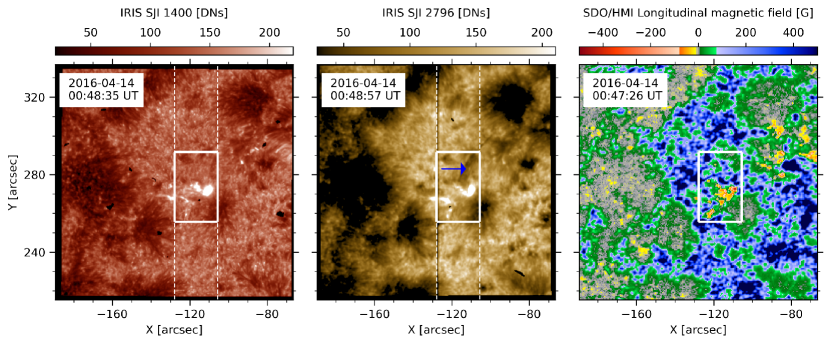
Figure 1: Context image of the events associated with the flux emergence region in the plage following the positive polarity of the AR NOAA 12529 at $\sim$00:48 UT on 2016 April 14. Left: IRIS SJI 1400 Å. Middle: IRIS SJI 2796 Å. Right: SDO/HMI line-of-sight (LOS) magnetogram. The vertical dashed lines indicate the area covered by the IRIS slit during the raster scans. The solid box, ranging from X=-127$\aas@@fstack{\prime\prime}$9 to X=-105$\aas@@fstack{\prime\prime}$6 and Y=255$\aas@@fstack{\prime\prime}$7 to Y=291$\aas@@fstack{\prime\prime}$6, frames the portion of the FoV studied in this paper. The blue arrow indicates one of the observed surges. The axes give the distance from solar disk center.

2.2 Methods

2.2.1 $k$-means clustering

$k$-means is an unsupervised clustering algorithm, popular in data-mining, machine learning, and artificial intelligence, that classifies a set of $n$ samples in $k$ disjoint groups (or clusters) of equal variance. To that end, it minimizes the within-cluster sum-of-squares (also known as inertia) given by

$$\sum_{i=1}^{n}\sum_{j=1}^{k}\min\left({\left|\left|x_{i}-\mu_{j}\right|\right|^{2}}\right),$$ (1)

where $x_{i}$ is the $i$-th observed point and $\mu_{j}$ the mean of the $j$-th cluster center or centroid.

This algorithm is relatively easy to implement, scales to large data sets and can be adapted to group line profiles. In solar physics, $k$-means has gained popularity being used, for instance, to classify Stokes profiles and chromospheric lines in different phenomena such as flares and spicules (see, e.g., Pietarila et al., 2007; Viticchié & Sánchez Almeida, 2011; Panos et al., 2018; Sainz Dalda et al., 2019; Bose et al., 2019; Robustini et al., 2019; Joshi et al., 2020a; Kuckein et al., 2020; Bose et al., 2021a, b; Barczynski et al., 2021).

In our case, we have used it to classify the Mg II h&k profiles obtained by IRIS within the subFoV shown as a solid box in Figure 1. This way, the $k$-means method can help us to identify whether surges have characteristic Mg II h&k line profiles that may indicate similar atmospheric properties. The reason to classify the spectra is inspired by the theoretical work by Nóbrega-Siverio et al. (2016), in which the authors discern different populations within the surge depending on the thermodynamics and evolution of the plasma. Details about the data processing to feed the $k$-means algorithm as well as the choice of the number of clusters $k$ can be found in Appendix A.

2.2.2 Inversions

Inversions of the Mg II h&k lines have been carried out using the STockholm inversion Code (STiC, de la Cruz Rodríguez et al., 2019, 2016), which assumes NLTE and includes partial frequency redistribution effects of scattered electrons (Leenaarts et al., 2012). This code allows us to get a stratified model of the solar atmosphere that covers, depending on the spectral lines considered to be inverted, the photosphere, the chromosphere, and the transition region. An initial guess model atmosphere is slightly modified in an iterative process until the output radiation, obtained by solving the radiative transfer equation taking the considerations mentioned above into account, fits the observed spectra. The interested reader in the problem of the inversion of spectral data in the context of the solar physics can find an excellent review by del Toro Iniesta & Ruiz Cobo (2016).

We also explored the possibility of inverting the Mg II h&k surge profiles using IRIS² (Sainz Dalda et al., 2019). Its inversion scheme (i.e., the number of nodes used in the thermodynamics variables to vary the model atmosphere at different optical depths) consists of two cycles: in the first cycle, it uses 4 nodes in temperature, and 3 nodes both in the line-of-sight and turbulent velocities; in the second cycle, it uses 7 nodes in temperature and 4 nodes in both velocities. Even though this approach is good enough for a large variety of profiles, it struggles with profiles with extreme line widths, such as those observed in X-class flares and UV bursts, and with profiles related to eruptive events. This means that the current version of IRIS² is not appropriated for phenomena like surges.

Nodes in variable for cycle #	1	2	3	4
$T$	4	7	9	9
$V_{turb}$	3	4	7	9
$V_{\mathrm{LOS}}$	3	4	4	6

Table 1: Number of nodes per cycle considered for the inversion of the Mg II h&k spectral profiles in this article.

Taking the above into consideration, we have proceeded to invert the Mg II h&k profiles of our observations with a more complex scheme than the one used to build the IRIS² database. After different tests, we have selected an inversion scheme that consists of 4 cycles whose details are summarized in Table 1. For cycles 1 and 2, the number of nodes are the same as those used to build the $IRIS^{2}$ database. The temperature, $T$, and electron density, $n_{e}$, in the initial guess model atmosphere for the cycle 1 are taken from the FALC model (Fontenla et al., 1993). The micro-turbulence velocity, $V_{turb}$, and the line-of-sight velocity, $V_{\mathrm{LOS}}$, are introduced ad-hoc as a smooth gradient along the optical depth between $-6\leq\log_{10}(\tau)\leq 0$ that goes from 3 to 1 km s^-1 for $V_{turb}$, and from 1 to 0.5 km s ^-1 for $V_{\mathrm{LOS}}$. The initial model atmosphere for the cycles 2, 3, and 4 is the output model atmosphere obtained from the previous cycle. The computation of the inversion uncertainties, $\sigma$, is carried out following Equation (42) of the paper by del Toro Iniesta & Ruiz Cobo (2016): the same calculation performed by Sainz Dalda et al. (2019) for the IRIS² database.

2.2.3 Density diagnostics

The density diagnostics method is based on the theoretical relationship between electron density and intensity ratio of the O IV 1399.8 Å and 1401.2 Å lines. Indeed, these intercombination lines are known to provide useful electron density diagnostics in a variety of solar features and astrophysical plasmas (see, e.g., Feldman & Doschek, 1979), because their ratios are largely independent of the electron temperature, and only weakly dependent on the electron distribution (Dudík et al., 2014). A recent discussion about the diagnostic potential of these lines in IRIS observations has been presented by Polito et al. (2016a), who also showed that their sensitivity interval for density diagnostics range between $10^{10}-10^{12}\,\mathrm{cm}^{-3}$.

The theoretical intensity ratios between the O IV 1399.8 Å and 1401.2 Å lines were used to derive the electron density from the observed line ratio, under the assumption of ionization equilibrium (CHIANTI v.8 database, Del Zanna et al., 2015), with formation temperature of $\log_{10}(T)=5.15$ K. We obtained the line peak intensity from each considered pixel by fitting a Gaussian function to the O IV 1399.8 Å and 1401.2 Å line profiles, respectively, also retrieving the uncertainties of the intensities. Blends in these emission lines are negligible in our study, as they mostly occur during flares (Polito et al., 2016b). Finally, for the computation of the density, we used the IDL SolarSoft routine iris_ne_oiv.pro.

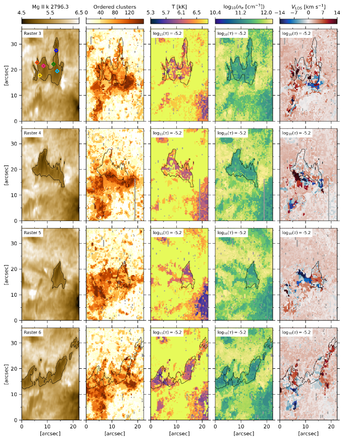
Figure 2: Observed surges and results from the $k$-means and inversions. From left to right columns: radiance maps in the core of the Mg II k 2796.3 Å line; cluster labels from the $k$-means ordered by the amount of profiles within a cluster; and maps at $\log_{10}(\tau)=-5.2$ for temperature, $T$, electron number density, $n_{e}$, and line-of-sight velocity, $V_{\mathrm{LOS}}$, from the inversions of the Mg II h&k line using the STiC code. Black contours delimit the bulk of the surges visible in the Mg II k 2796.3 Å radiance maps. Bad pixels and pixels affected by cosmic rays are masked and shown with color grey. Colored diamonds are superimposed in the first panel for later reference. An animation of this figure is available varying $\log_{10}(\tau)$ from $-6.0$ to $-3.2$.

2.3 Numerical experiments

To get a joint perspective between observations and theory, we have used three different 2.5D numerical experiments in which surges are ejected as a result of magnetic flux emergence. The simulations were performed with the radiation-magnetohydrodynamic Bifrost code (Gudiksen et al., 2011) assuming LTE and including thermal conduction along the magnetic field lines, optically thin losses, and radiation transfer adequate to the photosphere and chromosphere. The details of these simulations have been described in the papers by Nóbrega-Siverio et al. (2016, 2017, 2018).

3 Results

For the purpose of showing the surges analyzed in this paper, left column of Figure 2 contains radiance maps for the chromospheric Mg II k 2796.3 Å line within the selected subFoV (solid box in Figure 1) during the four IRIS raster scans. These maps are computed by averaging the intensity within $\pm 15\,\mathrm{km\,s}^{-1}$ with respect to the core of the aforementioned line. In the panels, we have added contours to ease the location of the bulk of the surges, which can be recognized by their dark and elongated structures composed by threads. The surges can be more extended spatially than the regions limited by these contours, since they refer only to the radiance maps in the center of Mg II k 2796.3 Å. In the panels, it is also possible to distinguish the location of the UV bursts associated with the surges, specially in the third and fourth rasters, due to their enhanced brightness (see Guglielmino et al., 2019b, for details about these UV bursts). In the following, we focus on the observed surges by studying their chromospheric properties through the Mg II h&k line (Section 3.1), analyzing their transition region counterpart using the O IV 1399.8 Å and 1401.2 Å lines (Section 3.2), and comparing the observational results with the simulations (Section 3.3).

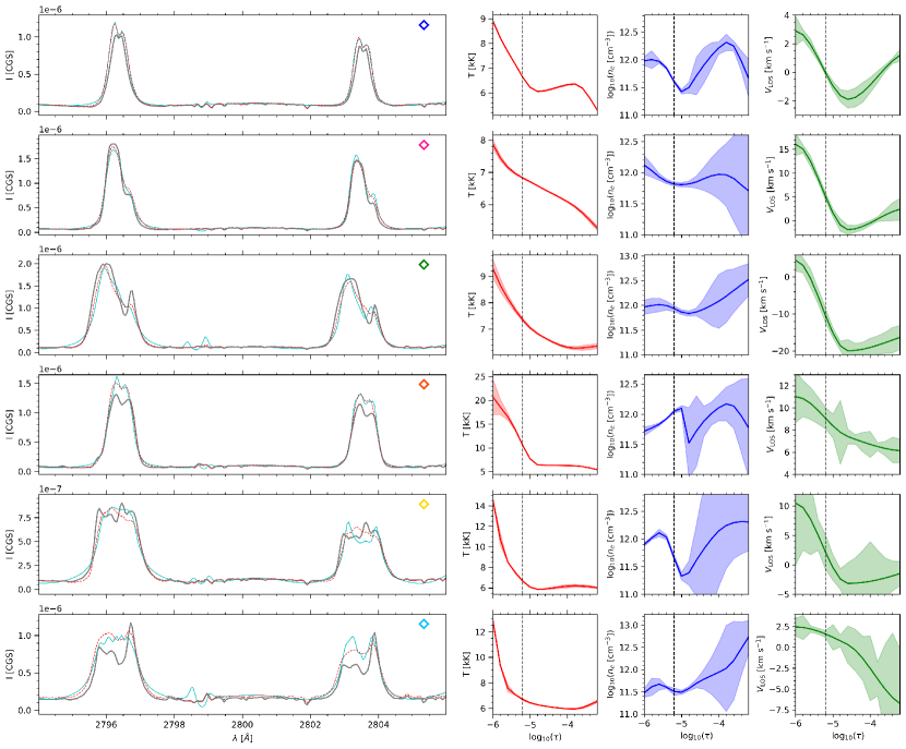
Figure 3: Spectral information and computed atmospheres for the six positions indicated with colored diamonds in Figure 2. Left column: observed Mg II h&k profile (grey line), corresponding representative profile obtained with the $k$-means method (red dashed line), and the inverted profile using the STiC code (cyan line) in CGS units (erg cm^-2 s^-1 sr^-1 Hz^-1). Three rightmost columns: results from the inversions for $T$ (red), $n_{e}$ (blue), and $V_{\mathrm{LOS}}$ (green) as functions of $\log_{10}(\tau)$ with their corresponding inversion uncertainties ($\pm\sigma$). The vertical dashed line in these plots at $\log_{10}(\tau)=-5.2$ indicates the optical depth shown in Figure 2

.

3.1 Analysis of Mg II h&k in the surges

3.1.1 Mg II h&k clustering and profile examples

The first step prior to analyze the Mg II h&k spectra within surges is the clustering through the $k$-means method (Section 2.2.1). In addition to identify representative profiles in the phenomenon of interest, this method allows us to noticeably reduce the number of Mg II h&k profiles that would be in principle necessary to analyze. In our particular case, we have chosen $k=160$ for each raster, thus getting a total of 640 representative profiles that are later inverted. This implies a reduction of a factor 43.2 with respect to the original total number of profiles (27648) within the IRIS subFoV chosen for this paper. Second column of Figure 2 contains the label maps of the clusters for each raster. The labels are assigned to the clusters depending on the amount of profiles that compose each clusters: lower the label number, greater the number of profiles in the corresponding cluster. By ordering the labels, we can already discern that surges and their surroundings have clear different Mg II h&k profiles from other regions.

In order to show the peculiarity of some of the surge profiles and to compare them with the representative ones obtained with the $k$-means, we have selected six different pixels in the surge of Raster 3 (colored diamonds in Figure 2), which are located in an elongated finger-like thread (blue); the left side of the bulk of the surge (pink); some particular regions at the boundaries of the ejection (orange, green and yellow); and the right side of the bulk of the surge (cyan). The later four locations are also used in the analysis of the O IV lines (Section 3.2). The Mg II h&k spectral profiles for these six locations are plotted in the left column of Figure 3 as grey lines. They show large diversity, with $k_{2V}$ and $h_{2V}$ peaks being greater than $k_{2R}$ and $h_{2R}$, respectively, excepting in the cyan location, suggesting different Doppler motions in the upper chromosphere (Leenaarts et al., 2013); $k_{3}$ and $h_{3}$ ranging from clearly visible valleys (as in the green location) to an almost flat behaviour (blue pixel); broad profiles with several peaks (yellow and cyan); and an interesting absence of emission in the Mg II triplet in all of them, which is contrarily observed in UV bursts (Hong et al., 2017). In the panels, we also plot, as a red dashed line, the corresponding representative profiles obtained with the $k$-means method. The representative profiles match quite well the observational data particularly for the blue, pink, orange and green locations, which only show slightly differences in the intensity while the shape of the Mg II h&k lines and the continuum are accurately represented. In the case of the cyan and yellow locations, the continuum and the width of Mg II h&k lines are properly captured with the representative profile; nonetheless, the shape of the peaks of the lines is less similar. We need to highlight that this discrepancy is a natural result expected from the $k$-means: there are always some observed profiles that are assigned to the cluster with the most similar profiles but still they are not nicely represented. In our case, we have checked that these divergent profiles represent a minority within the clusters (we have validated the good behaviour of the $k$-means algorithm by three different methods as mentioned in the Appendix A). Consequently, these small number of outliers have little impact on our results since we are interested in an overall view of the physical properties derived from inversions as discussed in the following section.

3.1.2 Inversions of the representative Mg II h&k profiles and statistics

Once we have the representative profiles for each raster, we proceed with their corresponding inversions using the state-of-the-art STiC code with the scheme explained in Section 2.2.2. Third, fourth and fifth columns of Figure 2 contain the results for the temperature, $T$; the electronic number density, $n_{e}$; and the LOS velocity, $V_{\mathrm{LOS}}$; respectively at $\log_{10}(\tau)=-5.2$. In the maps, it is possible to distinguish that the surges have some peculiarities in their physical properties such as they are mostly cooler and with smaller electron number density than their surroundings. With respect to the velocity, the maps reveal that the bulk of the surge have values of a few km s^-1, while the largest values are located next to the edges of the contours of the finger-like threads (see Raster 3 and 6) reaching up to $\sim 11$ km s^-1. An animation of this figure is also available, showing the variation of the properties with the optical depth between $-6.0\leq\log_{10}(\tau)\leq-3.2$.

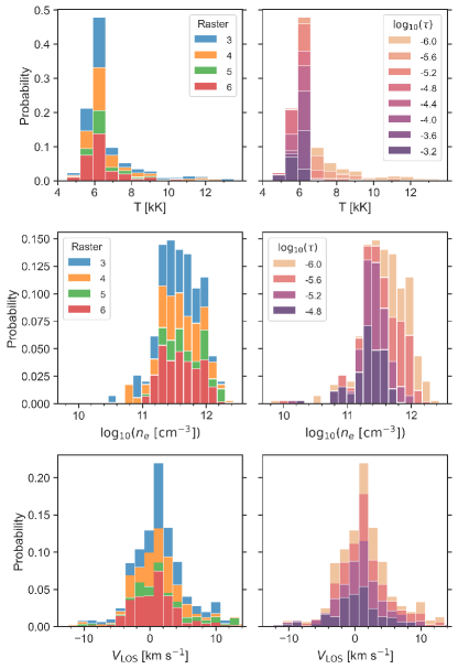
Figure 4: Statistical results for $T$ (top row), $n_{e}$ (middle row), and $V_{\mathrm{LOS}}$ (bottom row) obtained within the contour that delimits the bulk of the different surges in Figure 2. The statistics contain data from the optical depths where inversions are more reliable: from $\log_{10}(\tau)=-6.0$ to $-3.2$, for the temperature, and from $\log_{10}(\tau)=-6.0$ to $-4.8$ for the density and velocity. Left column: stacked histograms organized by raster showing that the different surges have similar properties. Right panel: stacked histograms organized by $\log_{10}(\tau)$ illustrating the variation of the physical parameters with the optical depth.

In the panels of the left column of Figure 3, we have plotted the inverted profiles for the selected locations of Raster 3 as cyan lines to compare them with the representative profiles obtained with the $k$-means method. This way, we can get an idea about whether the inversion scheme used in this paper (Table 1) is adequate for such complex profiles. We have found that, in most cases, the inverted profiles mimic the representative profiles with high grade of detail and that the major discrepancies are in the complex profiles of the cyan and yellow locations. Right panel of Figure 3 contains the corresponding representative model atmospheres extracted from the selected locations to illustrate the variation of $T$ (red), $n_{e}$ (blue), and $V_{\mathrm{LOS}}$(green) with $\log_{10}(\tau)$. For each physical quantity, we have also superimposed the inversion uncertainties ($\pm\sigma$ ). The uncertainties are small for the temperature in the whole range of optical depths, while for the density, the smaller uncertainties are located upper in the atmosphere (more negative values of $\log_{10}(\tau)$). The latter is also true for the velocity in the blue, pink, green and cyan locations. We have inspected the behaviour of the uncertainties for all the results within the black contour that delimits the bulk of the different surges in Figure 2, concluding that for the temperature, the accuracy of the inversions is excellent for all the optical depths within $\log_{10}(\tau)=-6.0$ and $-3.2$; for the density, the inversions results can be rather acceptable between $\log_{10}(\tau)=-6.0$ and $-4.8$; and for the velocities, the range between $\log_{10}(\tau)=-6.0$ and $-4.8$ is also the best one generally.

To get a whole perspective of the general properties of the surges, we need to perform a statistical analysis. Figure 4 contains histograms for $T$ (top row), $n_{e}$ (middle row), and $V_{\mathrm{LOS}}$(bottom row), obtained within the black contour that delimits the bulk of the different surges in Figure 2. To create these histograms, we consider the range of optical depths in which the uncertainties are smaller for each physical quantity. The histograms in the left column of the figure are stacked by rasters, that is, each bar in the chart represents a whole, and the length of the segments in the bar represents the contribution from each raster to the whole. Even though we have performed $k$-means individually for each raster with topologically different surges, the statistical distributions for temperature, density and velocity that we obtain after the inversions of the representative profiles are very similar: an important result that confers robustness to our method to characterize the properties of the surges. The characteristic properties of our surges are as follows: the most probable temperature is around $6$ kK, the electronic number density is mostly concentrated from $\sim 1.6\times 10^{11}$ to $10^{12}$ cm^-3, and the LOS velocity is typically of a few km s^-1. The right column of Figure 4 shows the same statistics but stacked by optical depth, highlighting the variation of the parameters with the optical depth. In this case, cooler plasma with smaller electron number density in the surges is located at less negative values of the optical depth, that is, deeper in the atmosphere.

3.2 Analysis of O IV in the surges

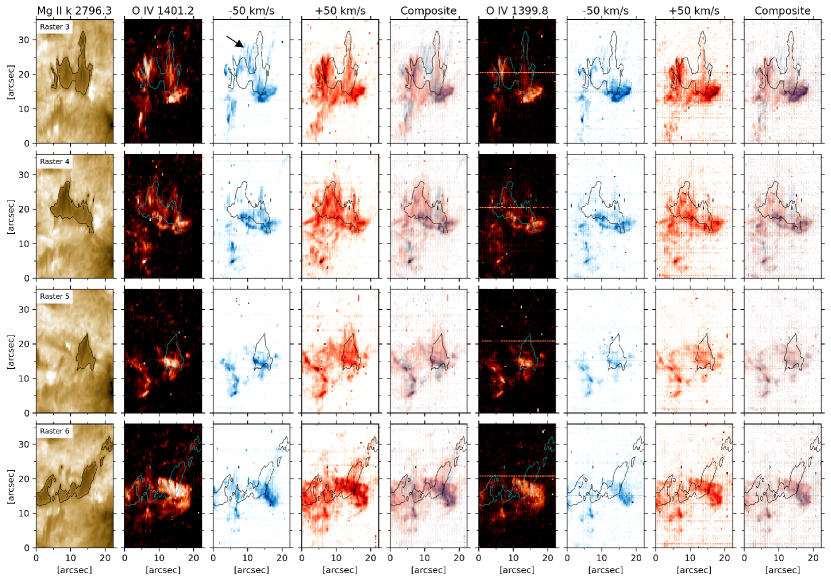
Figure 5: Radiance maps showing the O IV emissivity of the surges. From left to right: radiance maps in the core of the Mg II k 2796.3 Å line (first column); in the core of the O IV 1401.2 Å line (second column); in the blue and red wings at $-50$ and $50\,\mathrm{km\,s}^{-1}$ of O IV 1401.2 Å (third and fourth columns, respectively); and composite image of the blue and red wing radiance maps for O IV 1401.2 Å (fifth column). Equivalent maps are plotted for the O IV 1399.8 Å line (sixth-ninth columns). The contours in all the panels delimit the bulk of the surges visible in the Mg II k 2796.3 Å radiance maps. The black arrow in the third panel of the first row indicates the location of enhanced O IV emission associated with finger-like threads of a surge. The O IV maps show a horizontal strip of hot pixels that does not affect our findings.

3.2.1 Enhanced O IV emissivity within the surge

One of the most striking results is the finding, for the first time, of emission in the O IV 1401.2 Å and O IV 1399.8 Å lines in surges. To illustrate this fact, Figure 5 contains the Mg II k 2796.3 Å line radiance maps for the four rasters (first column), to show the context, and the corresponding radiance maps for O IV 1401.2 Å (second column) and for O IV 1399.8 Å (sixth column). These radiance maps are computed by averaging the intensity within $\pm 15\,\mathrm{km\,s}^{-1}$ with respect to the core of each line. In addition, for both O IV lines, we compute maps of integrated emission in the blue wing at $-50\,\mathrm{km\,s}^{-1}$ (third/seventh column of the figure) and in the red wing at $+50\,\mathrm{km\,s}^{-1}$ (fourth/eighth column). Differences in the location of the emitting regions between the wings are determined from the composite maps (fifth/ninth column of the image). To ease the identification, all the panels show contours that delimit the bulk of the surges visible in the Mg II k 2796.3 Å radiance maps. The maps, specially the radiance ones of O IV 1399.8 Å, contain a horizontal strip of hot pixels; however, this does not affect our results.

Inspecting the image, we can see that both O IV 1401.2 Å and O IV 1399.8 Å radiance maps at the center of the line (second and sixth columns) look quite similar, although the surges appear to have a larger extension in O IV 1401.2 Å than in O IV 1399.8 Å, likely due to the fact that the former is a stronger line. The location of the brightest O IV regions can be found within the bulk of the surges and/or in their boundaries following the threads of the surges. This is particularly evident in the third and fourth rasters. The corresponding blue/red wing and composite maps also provide evidences about the transition region counterpart of the surges in these weak O IV lines. For instance, in the third panel of the first row of the image, a black arrow indicates the location of enhanced O IV emission associated with finger-like threads of the surge. In addition, the maps also reveal a peculiar behavior in these threads: while several threads are observed co-located both in the blue and red wings of the O IV lines, some others show a significant shift in the position where they are detected in the blue and red wings of those lines. This asymmetry is similar to the noticed for Mg ii k and Si IV 1402.8 Å lines by Guglielmino et al. (2019b) and it could be an evidence of helical/rotational motions typically associated with surges.

3.2.2 Spectral analysis and density diagnostics

To know how the O IV spectra related to the surges look like, left panel of Figure 6 contains the O IV 1401.2 Å radiance map with reversed color scale for the third raster. From our previous choice of locations in Figure 2, we have selected the pixels with strong intensity in both O IV lines (orange, yellow, green, and cyan diamonds). In addition, we also consider some other pixels along a thread of the surge, approximately located at $x=6\arcsec$ and $y\in[20\arcsec,25\arcsec]$, that have the greatest O IV intensity (orange and magenta segments). The black diamond in the map indicates a quiet-Sun area with a vertical segment of six pixels in which the spectrum has been averaged for comparison purposes. The corresponding surge and quiet-Sun spectra are shown in the middle panel of Figure 6 using the same colors as for the diamonds. In this panel, we can see that the O IV intensity associated with the surge is a factor between 7 and 15, for the O IV 1399.8 Å line, and between 12 and 35, for the O IV 1401.2 Å line, brighter than the quiet-Sun average profile: surges have a transition region counterpart even in the weakest FUV lines. This is moreover very different from UV bursts, where the O IV 1401.2 Å line is very weak in comparison to Si IV 1402.8, and the O IV 1399.8 Å line is absent (Peter et al., 2014; Young et al., 2018). With respect to the Si IV 1402.8 intensity, the ratio between the surge and the quiet-Sun region intensities ranges from  2.5 to 6.5, which agrees with the values previously found in IRIS observations (from 2 to 5) by Nóbrega-Siverio et al., 2017.

The simultaneous finding of O IV 1399.8 Å and 1401.2 Å allows us to estimate the electron density in the transition region of the surges. Applying the density diagnostics method described in Section 2.2.3 for the selected pixels (diamonds and vertical segments in the left panel of Figure 6), we obtain a density in the range of $\approx 2.5\times 10^{10}-10^{12}\,\mathrm{cm}^{-3}$ as shown in the right panel of Figure 5, where the yellow pixel lies at the high-density limit of the diagnostic method.

The next question to address is whether it is possible to establish a connection between the physical quantities that are derived for the transition region from the O IV analysis and the ones obtained for the mid- and low-chromosphere in Section 3.1.2 from the Mg II h&k lines. The green location, for instance, shows an O IV spectrum (middle panel of Figure 6) that appears to be taken in a pixel almost at rest, while the electron density (right panel of Figure 6) is around $2\times 10^{11}\,\mathrm{cm}^{-3}$. For this location, the Mg II h&k inversions (Figure 3) show that, at $\log_{10}(\tau)=-6$, the velocity is small ($\sim 1\pm 1$ km s^-1), which is consistent with the Doppler shift found in O IV, and the density is close to $10^{12}\,\mathrm{cm}^{-3}$ and decreases towards higher layers in the atmosphere, which also seems to be consistent if we assume that the O IV information comes from an upper and more rarefied layer. The orange pixel has an O IV spectrum exhibiting a slight redshift of about $10\,\mathrm{km\,s}^{-1}$ and a density of $\approx 8\times 10^{10}\mathrm{cm}^{-3}$. This also appears to be in agreement with the results from the inversions, which show redshift velocities of $\sim 11\pm 3\,\mathrm{km\,s}^{-1}$ and a density of $5\times 10^{11}\,\mathrm{cm}^{-3}$ rapidly decreasing upwards. The yellow and cyan locations show both redshifts in O IV, being the yellow location the one with larger velocities and more electron density. This general behavior is also found in the inversions, although the comparison is more complicated owing to the uncertainties involved in these two locations. In the following section, we compare these results with those from numerical simulations.

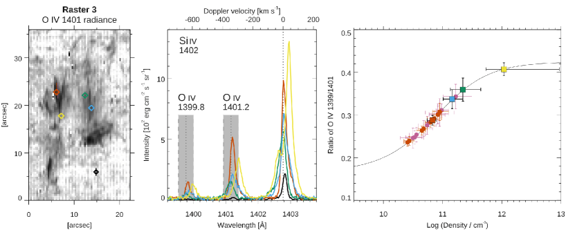
Figure 6: O IV spectral analysis and density diagnostics. Left: O IV 1401.2 Å radiance map (reversed color scale) for the third raster with superimposed colored diamonds (orange, green, blue, and yellow) and colored segments (orange and magenta) where the spectra are analyzed. For reference, the black diamond illustrates a quiet-Sun area with a vertical segment of six pixels in which the quiet-Sun spectrum has been averaged. Middle: FUV spectra in the Si IV 1402 Å passband for the positions indicated in the left map with diamonds. Grey shaded areas delimit spectral regions at $\pm 50\,\mathrm{km\,s}^{-1}$ encompassing O IV 1399.8 Å and O IV 1401.2 Å lines. Right panel: Results from the density diagnostics using the O IV 1399.8/1401.2 ratio for the surge pixels selected in the left panel.

3.3 Comparison between observations and numerical experiments

To get a joint perspective between observations and theory, Figure 7 contains electron number density maps for three different 2.5D numerical experiments at the time when surges are at their apex. The ejections are discernible as elongated structures and their locations are indicated with arrows. The three surges show finger like structures similar to the observed ones. It is also possible to distinguish, specially in the left panel, that $n_{e}$ shows variations within the surge that look like threads. Temperature contours are superimposed for $T=6$ kK (green), $T=10$ kK (blue) and $T=200$ kK (red), highlighting the multi-thermal structure of these phenomena. Focusing on the location of these contours, we can see that in some regions of the surge there are large temperature gradients with cool chromospheric plasma being close to the transition region plasma (where O IV emission is originated), while in other regions, the transition region of the surge is far away (from hundred km up to a few Mm) from the cool core. This may explain why the location of the observed brightest O IV regions in Figure 5 can be found within the bulk of the surges and/or in their boundaries following the threads of the surges. Around the $T=6$ kK contour, the surges have a clear core with small electron number density. The number density increases from the core outwards until reaching transition region, where it decreases again. Table 2 contains the averaged $n_{e}$ in the temperature contours for the three experiments as a zero order approximation to compare with the observations. By doing this, we obtain number densities that are lower than those derived from observations. This means that, although qualitatively the experiments help us to understand the observed features, for a more accurate comparison we would need to include nonequilibrium effects to properly model the chromosphere and synthesize Mg II h&k lines in the experiments (see Discussion).

$\log_{10}(n_{e}$ [cm-3])	Exp. A	Exp. B	Exp. C
at $T=6\mathrm{kK}$	$10.6$	$10.8$	$10.5$
at $T=10\mathrm{kK}$	$11.4$	$12.7$	$12.5$
at $T=200\mathrm{kK}$	$9.6$	$9.3$	$9.5$

Table 2: Averaged electron number density in the temperature contours of the numerical experiments shown in Figure 7.

4 Discussion and conclusions

In this paper, we have used observations from the IRIS satellite to study an episode of recurrent surges that appear associated with UV bursts in Active Region (AR) NOAA 12529 on 2016 April. This is the first study of surges that characterizes their fundamental properties using the Mg II h&k as well as the O IV 1399.8 and 1401.1 Å spectral lines, combining to that end different methods such as the $k$-means algorithm, inversions with the STiC code, and density diagnostics. In addition, we have employed numerical experiments using the Bifrost code to get a qualitative comparison between observations and theory. In the following, we summarize and discuss the main findings of this paper.

In Section 3.1, we have analyzed the near-UV spectra of surges through the Mg II h&k line, focusing on the properties of the surges as they have been mainly unexplored. In Section 3.1.1, we have used the $k$-means method in each of the four selected rasters to find Mg II h&k representative profiles in our observation and invert them. Thanks to this method, we reduce the number of profiles to invert by a factor 43.2, thus alleviating the computational and analysis effort, as well as being able to discern regions with peculiar profiles, like in the case of surges and UV bursts. The $k$-means algorithm is not the only approach for this kind of studies. For instance, Verma et al. (2021) employ $t$-distributed stochastic neighbor embedding (t-SNE), another machine learning algorithm, to classify the H$\alpha$ spectra with the aim of separating different regions to perform cloud model inversions. In Section 3.1.2, we have inverted our representative profiles from the $k$-means finding that the surges have their most probable temperature around $6$ kK, electronic number densities mostly concentrated from $\sim 1.6\times 10^{11}$ to $10^{12}$ cm^-3, and LOS velocities of a few km s^-1. In addition, we have also showed that the statistical distributions of these properties are very similar for the different surges, meaning that these ejections can be well constrained in terms of their physical quantities. The uncertainties analysis show that the values of temperature for the surges are very reliable for optical depths between $\log_{10}(\tau)=-6.0$ and $-3.2$, the density values can only be considered between $\log_{10}(\tau)=-6.0$ to $-4.8$, while the velocities are generally acceptable also between $\log_{10}(\tau)=-6.0$ to $-4.8$, although it is preferred to examine them individually pixel by pixel. These results have allowed us not only to gain new insights of fundamental properties of the surges, but also to constitute the first steps to characterize the surge spectral profiles in the main chromospheric lines in which they are observed. To the best of our knowledge, there is only one paper (Kejun et al., 1996) in which physical parameters of surges are computed through a two-component cloud model using H$\alpha$, obtaining $T=8.5$ kK and $n_{e}=1.8\times 10^{10}$ cm^-3. More recently, inverting the Ca II 8542 Å line using the NLTE code NICOLE, Kuridze et al. (2021) obtain the electron density values of a large spicule off the limb. Their results show that $n_{e}$ ranges from $2.5\times 10^{13}$ cm^-3, at the spicule bottom, to $\sim 2\times 10^{10}$ cm^-3, at its top. They argue that the density obtained is more akin to surges rather than typical spicules. In our case, the results from the inversion reveal a more constrained range for the electronic number density.

Figure 7: Electron number density for three different simulated surges. Contours of temperature are superimposed for $T=6$ kK (green), $T=10$ kK (blue) and $T=200$ kK (red). Panel A: surge from the Nóbrega-Siverio et al. (2016) numerical experiment. Panels B and C: surges from the simulations by Nóbrega-Siverio et al. (2017, 2018).

In Section 3.2, we have focused on the transition region counterpart of surges through the FUV spectra. Thanks to the relatively long exposure time used in the IRIS sequence (18 s for FUV, thus ensuring good signal-to-noise ratio for faint lines in the transition region), in Section 3.2.1 we have been able to find emission in the O IV 1399.8 Å and 1401.1 Å lines related to the surges. This finding is relevant due to the following reasons: i) this is the first observational report of O IV 1399.8 Å and 1401.1 Å related to surges, in fact, previous FUV analysis could not detect any O IV emission because the exposure time was too short (Nóbrega-Siverio et al., 2017), or because the focus was on other lines (Guglielmino et al., 2019b); ii) it clearly demonstrates that surges have a transition region counterpart even in the weakest FUV lines (the oscillator strength, which is proportional to the line strength, of 1401.1 Å is $5.1\times 10^{-7}$ and the one for O IV 1399.8 Å is $4.3\times 10^{-7}$, which is a 16% smaller); iii) it gives observational support to the theoretical findings by Nóbrega-Siverio et al. (2018), which showed that the surges can have enhanced emissivity in lines like O IV 1401.1 Å. We have also found that surges have threads with important blue- and redshifts that can appear spatially displaced (see composite maps of Figure 5). This could be an indication of helical/rotational motions in the transition region counterpart of the surges during their untwisting and ejection. Similar asymmetry in the locations of the blue- and redshifts within surges is also found in the Mg ii k and Si IV 1402 Å lines by Guglielmino et al. (2019b), and they join to the further indications of rotational motions associated with surges described previously in the literature (see, e.g., Canfield et al., 1996; Jibben & Canfield, 2004; Jiang et al., 2007; Bong et al., 2014). In Section 3.2.2, we have selected the brightest O IV pixels in the surge to perform density diagnostics, finding that the electron number density ranges from, approximately, $2.5\times 10^{10}$ to 10¹² cm^-3. The physical quantities obtained from O IV seem to be consistent with those derived from Mg II h&k inversions for these locations. However, one has to be cautious: the O IV intensity we observe can come from the integration along the LOS of different regions of the surge, as shown in numerical experiments by Nóbrega-Siverio et al. (2018), so the inferred electron density could be just a weighted mean average electron density along the line of sight. In addition, nonequilibrium ionization can be relevant for these emitting layers, and density diagnostics may be affected by an order of magnitude (Olluri et al., 2013). A possible way of better constrain the physical properties of surges in the future is using inversions combining the information from the chromosphere and transition region in a similar fashion as Vissers et al. (2019) carried out for UV bursts and Ellermam bombs.

In Section 3.3, we qualitatively compare three simulations with the observations finding similarities in terms of the topology that may also explain the location of the observed brightest O IV regions with respect to the bulk/core of the surges. Nóbrega-Siverio et al. (2016) show that the bulk of their simulated surge (population A in that paper) is quite concentrated around $6$ kK, which agrees with the values from the inversions we find here. The electron number density, instead, seems to be lower in the simulations. This could be related to the lack of nonequilibrium ionization in these experiments. Nóbrega-Siverio et al. (2020) demonstrate that the LTE assumption substantially underestimates the ionization fraction in most of the emerged region, which could lead to lower electron number densities in the subsequent surge. Therefore, numerical simulations of surges including the ionization out-of-equilibrium of hydrogen seems mandatory to match the physical properties derived from observations.

The combination of methods and results obtained in this paper open new possibilities for the analysis and diagnostics of surges. For instance, our inverted representative profiles and their corresponding representative model atmospheres will be included in the IRIS² (Sainz Dalda et al., 2019) database, improving its current capabilities to invert eruptive phenomena. These results may facilitate building automatic detection algorithms for these key ejections in observations. The simultaneous inversions of different spectral lines in which surges are observed will also allow us to compare and better constrain numerical experiments. In this vein, in the near future we expect to exploit the existing high-quality data by the Swedish 1-m Solar Telescope (SST) to perform detailed characterization of surges in other lines such as Ca II H&K and Ca II 8542 Å (see, e.g., the publicly available co-aligned IRIS and SST datasets by Rouppe van der Voort et al., 2020) . In addition, future observations from, for instance, the SPICE instrument on board the Solar Orbiter mission (Spice Consortium et al., 2020) could help us to continue exploring the upper chromosphere and transition region of these important phenomena through lines such as H I 1025.7 Å, $\log_{10}(T)=4$ K; C III 977.0 Å, $\log_{10}(T)=4.5$ K; and O VI 1031.9 Å, $\log_{10}(T)=5.5$ K. In the same way, the 4-m diameter Daniel K. Inouye Solar Telescope (DKIST, Rimmele et al., 2020) could offer potential diagnostics at upper chromosphere and transition region temperatures of surges, for example, in the He I D3 and 10830 Å lines.

Appendix A Processing for the $k$-means algorithm

To obtain meaningful results out of the $k$-means clustering, it is necessary to process the observational data properly. To that end, we have carried out the following steps.

1. Selection of the domain. We have chosen the subFoV of Figure 1 for our $k$-means clustering, thus reducing the number of profiles to be grouped that are not the aim of this paper.

2. Removing bad data. Any profile affected by data loss or cosmic rays is replaced by zero values. This is helpful as a benchmark: our data has 327 profiles affected and the $k$-means group them together in one single cluster, thus being able to easily mask them in the figures of the paper.

3. Radiometric calibration. We have performed radiometric calibration of the observational data to convert them into physical units. This step is essential to use the results obtained by the $k$-means method as input for the inversions.

4. Cropping the spectra. We have cropped the spectra to the range between 2794 to 2806 Å, which is sampled with 237 points. This is enough to contain the whole Mg II h&k line. Top panel of Figure 8 shows the distribution of all the calibrated profiles through a joint-PDF plot as well as the average profile (dashed line).

5. Standardization of individual features. This step is a common requirement for machine learning estimators to avoid bad behavior if the features are not more or less normally distributed. Our features are the wavelength positions, so for all the 237 positions between 2794 to 2806 Å, we have carried out a standardization of the intensity.

After processing all the data, we have performed the $k$-means method using the tools available on Scikit-learn (Pedregosa et al., 2011) and selecting 160 clusters for each of the four rasters. The initialization of clusters is repeated 100 times, keeping the best output of the consecutive runs in terms of inertia. We have concluded that $k=160$ is an appropriate number of clusters through three different methods: visual comparison of the representative profiles with the observed profiles belonging to a given cluster through joint-PDFs; using the benchmark of the bad pixels mentioned before; and checking the behavior of the inertia with the number of clusters (the elbow technique shown in bottom panel of Figure 8). In the figure, the regime $k\gtrsim 80$ shows little variation of the inertia for the four rasters. Since our purpose are inversions and not finding the minimum number of clusters in which the data can be grouped, we can take any $k$ in this regime because the inversions will give very similar results.

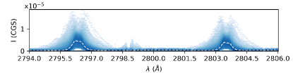
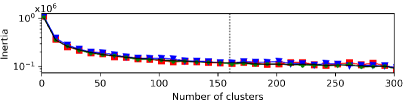
Figure 8: Data information for the $k$-means clustering. Top: Joint-PDF of all the calibrated Mg II h&k line profiles in CGS units (erg cm^-2 s^-1 sr^-1 Hz^-1) within the subFoV of Figure 1 for the four rasters. The corresponding average profile is shown as a dashed line. Bottom: Behavior of the inertia of the $k$-means method with increasing clusters to choose a suitable number through the elbow technique for raster 1 (red square), raster 2 (blue triangle), raster 3 (green circle), raster 4 (black line). Our cluster choice for all the rasters, $k=160$, is indicated by the vertical line.