Abstract

Polarized synchrotron emission from the radio halos of diffuse intracluster medium (ICM) in galaxy clusters are yet to be observed. To investigate the expected polarization in the ICM, we use high resolution ($1$ kpc) magnetohydrodynamic simulations of fluctuation dynamos, which produces intermittent magnetic field structures, for varying scales of turbulent driving ($l_{\rm f}$) to generate synthetic observations of the polarized emission. We focus on how the inferred diffuse polarized emission for different $l_{\rm f}$ is affected due to smoothing by a finite telescope resolution. The mean fractional polarization $\langle p\rangle$ vary as $\langle p\rangle\propto l_{\rm f}^{1/2}$ with $\langle p\rangle>20\%$ for $l_{\rm f}\gtrsim 60$ kpc, at frequencies $\nu>4\,{\rm GHz}$. Faraday depolarization at $\nu<3$ GHz leads to deviation from this relation, and in combination with beam depolarization, filamentary polarized structures are completely erased, reducing $\langle p\rangle$ to below 5% level at $\nu\lesssim 1$ GHz. Smoothing on scales up to $30$ kpc reduces $\langle p\rangle$ above $4$ GHz by at most a factor of 2 compared to that expected at $1$ kpc resolution of the simulations, especially for $l_{\rm f}\gtrsim 100$ kpc, while at $\nu<3$ GHz, $\langle p\rangle$ is reduced by a factor of more than 5 for $l_{\rm f}\gtrsim 100$ kpc, and by more than 10 for $l_{\rm f}\lesssim 100$ kpc. Our results suggest that observational estimates of, or constrain on, $\langle p\rangle$ at $\nu\gtrsim 4$ GHz could be used as an indicator of the turbulent driving scale in the ICM.

xx 1 5 Academic Editors: Received: date; Accepted: date; Published: date Properties of Polarized Synchrotron Emission from Fluctuation Dynamo Action – II. Effects of Turbulence Driving in the ICM and Beam Smoothing Aritra Basu^1,†*, Sharanya Sur ^2,†,* Aritra Basu and, Sharanya Sur Correspondence: abasu@tls-tautenburg.de, sharanya.sur@iiap.res.in These authors contributed equally to this work.

1 Introduction

Galaxy clusters are the largest known gravitationally bound systems which provide important clues on how structures were formed in the Universe. Besides gravity, magnetic fields are also believed to play an important role in the evolution of the intracluster medium (ICM) of galaxy clusters which emit in the radio and X-ray wavebands. A large fraction of massive merging clusters show diffuse radio emission (radio halo) originating from relativistic electrons, possibly accelerated by turbulence in the ICM, illuminating the cluster magnetic fields via synchrotron radiation (Feretti et al., 2012; van Weeren et al., 2019). This emission is expected to be partially polarized, and its measurement provides insights into the statistical properties of magnetic field structure in the ICM (Vazza et al., 2018; Domínguez-Fernández et al., 2019; Sur et al., 2021). So far, microgauss ($\upmu$G) strength magnetic fields ordered on several kpc scales in halos have been indirectly inferred via Faraday rotation measure (RM) estimated towards polarized sources located in the background, or from depolarization studies of radio relics, remnants of cluster collisions (Clarke et al., 2001; Bonafede et al., 2009, 2010; Kierdorf et al., 2017). In the absence of large-scale rotation of the ICM, such field strengths can naturally arise from fluctuation dynamo action where dynamically insignificant seed magnetic fields are amplified by random stretching of the field by turbulent eddies (Subramanian et al., 2006; Cho and Ryu, 2009; Bhat and Subramanian, 2013; Porter et al., 2015; Vazza et al., 2018; Sur et al., 2018; Sur, 2019; Sur et al., 2021). Understanding the structural and coherence properties of these fields is important as they contribute to pressure balance, control the acceleration and propagation of relativistic particles (Brunetti and Jones, 2014), and possibly play an important role in governing microphysical processes such as thermal conduction, spatial mixing of gas and kinetic viscosity (Kunz et al., 2011; Komarov et al., 2014; Roberg-Clark et al., 2016). A direct detection of polarized halo emission remains elusive and is a major science driver for the Square Kilometre Array (SKA) later this decade, e.g., (Bonafede et al., 2015).

Tentative detection of polarized emission for only three clusters have been reported, namely, for Abell 2255 (Govoni et al., 2005), MACS 0717.5+3745 (Bonafede et al., 2009), and Abell 523 (Girardi et al., 2016). It is likely that for all the three cases the polarized signal is related to a radio relic seen in projection rather than the halo emission itself (Pizzo et al., 2011; Rajpurohit et al., 2021). It is noteworthy that all three reports of polarized halo emission are based on observations at 1.4 GHz, a frequency at which many radio relics show polarized emission (Wittor et al., 2019). Due to the large Faraday dispersion in the ICM, Böhringer et al. (2016) found that the presence of a cluster medium increases the Faraday depth dispersion ($\sigma_{\rm FD}$) by about 60 rad m^-2, and therefore, polarized halo emission is expected to be highly depolarized at 1.4 GHz. Hence, no clean detection of diffuse polarized halo emission has been made so far.

Most of the previous attempts to constrain magnetic fields in the ICM by using RM measured towards polarized background sources and/or depolarization of cluster radio sources are based on the assumption of Gaussian random fields, e.g., (Bonafede et al., 2010; Vacca et al., 2010). However, in stark contrast, numerical magnetohydrodynamic (MHD) simulations reveal that fluctuation dynamo-generated fields are spatially intermittent (Schekochihin et al., 2004; Brandenburg and Subramanian, 2005; Vazza et al., 2018; Seta et al., 2020; Sur et al., 2021) with the field components exhibiting non-Gaussian distributions. In order to maximize the chance to confidently detect polarized emission from cluster halos using current and/or future radio telescope facilities, it is therefore imperative to investigate the expected polarized signal directly from fluctuation dynamo-generated fields obtained in MHD simulations. To this end, to gain information on the properties of polarized synchrotron emission from intermittent magnetic fields amplified by fluctuation dynamo, we have recently performed realistic broad-bandwidth, synthetic observations using MHD simulations of ICM see Sur et al. (2021), for details. Here, to mimic cluster merger-driven turbulence, also the same process which produces the radio halo, incompressible turbulence is solenoidally forced on 256 kpc for a simulation box-size of 512 kpc giving rise to magnetic fields ($B$) being correlated on $\sim$110$\,{\rm kpc}$ (also indicated by cosmological simulations; Domínguez-Fernández et al. (2019)). This results in polarized intensity, ${\rm PI}\propto\int B^{2}\,{d}l$, correlated on $\sim$200 kpc scales. However, due to strong Faraday depolarization at frequencies below $\sim$3 $\,{\rm GHz}$, polarized structures on significantly smaller scales are produced. These simulations roughly correspond to the central regions of massive Coma-like galaxy-clusters. The main outcome from the work of Sur et al. (2021) is that, one needs high frequency ($\nu\gtrsim 5\,{\rm GHz}$) observations to detect polarization in cluster radio halos, and with high spatial resolution ($\approx$1 $\,{\rm kpc}$) to infer its structural properties.

In this paper, we expand the scope of our work and present detailed investigation of the effects of turbulent driving at different scales on the properties of the polarized synchrotron emission when smoothed by a telescope beam at three representative frequencies of 0.6, 1.2 and 5 GHz. These frequencies represent the typical frequencies at which galaxy clusters are observed, and also corresponds to Band 1 (covering 0.35–1.05 GHz), Band 2 (covering 0.95–1.76 GHz), and Band 5 (covering 4.6–15.3 GHz) of the SKA’s mid-frequency component, SKA1-MID. A key question which we seek to address using the synthetic observations concerns whether the mean fractional polarization can inform us about the turbulent driving scale in the ICM. To investigate the effects different scales of turbulent forcing have on the polarized emission in the ICM, in this work, we forced turbulence on scales of $256,102$ and $64\,{\rm kpc}$ which gives rise to magnetic field structures correlated on widely different scales. For a representative cluster like Coma, these roughly correspond to scales ranging from the core radius down to scales of pressure scale-height. Magnetic fields generated by fluctuation dynamos can be ordered at the most on the scale of turbulent motions. Consequently, turbulent driving on the aforementioned scales enables us to probe the statistical properties of the polarized emission due to random magnetic fields with varying correlation lengths. This paper is structured as follows: in Section 2, we present in brief the details on the numerical simulations and methodology of obtaining synthetic observations from the simulation data. In Section 3, we discuss the results by first focusing on the power spectra of the kinetic and the magnetic energies, and that of the Faraday depth (FD). Next, we analyze the statistical properties of the total and polarized emission in radio halos when synthetic observations are smoothed over various scales to study the impact of telescope beam. We focus on the dependence of the mean fractional polarization of the diffuse ICM on the turbulent driving scale. Finally, in Section 4 we conclude with a summary of the main results and discuss the implications of our work on the properties of polarized emission in the ICM.

2 Methodology of Numerical Calculations

In this section, we present in brief the setup used for performing direct numerical MHD simulations, and the methodology of computing the synthetic observations using the simulation data. For further detail on these methods, we refer an interested reader to Sur (2019); Basu et al. (2019) and Sur et al. (2021).

2.1 Summary of Magnetohydrodynamic (MHD) Simulations

In this work, we make use of numerical simulations of fluctuation dynamos performed with the FLASH code (Fryxell et al., 2000) to address the aforementioned goals of this work. We focus on three simulations performed with an isothermal equation of state where turbulence is driven non-helically at three different forcing wave numbers, $k_{\rm f}L/2\pi=2,5$ and $8$, referred to as run A, B and C, respectively, in Table 1. The setup of each of these simulations is identical to the one presented in Sur et al. (2021). We therefore highlight only the essential features here. All the three simulations are performed at magnetic Prandtl number $\rm Pm=\rm Rm/{\rm Re}=1$, where $\rm Rm$ and ${\rm Re}$ are the magnetic and fluid Reynolds numbers, respectively. Recent cosmological simulations of hierarchical structure formation including the formation of galaxy clusters show that turbulence in the cluster core is dominated by solenoidal modes (Miniati, 2015; Vazza et al., 2017; Wittor et al., 2017; Vallés-Pérez et al., 2021). Accordingly, and to maximize the efficiency of the fluctuation dynamo, we use only solenoidal modes (i.e., $\nabla\cdot\mbox{\boldmath$F$}{}=0$) for the turbulent driving. Here, $F$ is the forcing term in the MHD equations. Furthermore, we adjust the amplitude of the forcing such that the resulting root mean square (rms) value of the Mach number $\mathcal{M}=u_{\rm rms}/c_{\rm s}\approx 0.18\textrm{--}0.19$, where $c_{\rm s}$ is the isothermal sound speed, and $u_{\rm rms}$ is the rms velocity. The subsonic nature of these simulations imply that density fluctuations ($\delta\rho/\rho\approx\mathcal{M}^{2}$) are negligible. This is in accordance with observational results which show rms turbulent velocity of $\approx$200–300 $\,{\rm km\,s^{-1}}$ (Hitomi Collaboration: Aharonian et al., 2018), and density fluctuations, inferred from X-ray surface brightness fluctuations, are at a $7\textrm{--}10\%$ level on scales of $\sim$500 $\,{\rm kpc}$ (Churazov et al., 2012), down to $\sim$4% on scales of $30\textrm{--}50\,{\rm kpc}$ (Zhuravleva et al., 2019). Our simulations were initialized with weak seed magnetic fields of the form ${\mathchoice{\mbox{\boldmath$\displaystyle B$}}{\mbox{\boldmath$\textstyle B$}}{\mbox{\boldmath$\scriptstyle B$}}{\mbox{\boldmath$\scriptscriptstyle B$}}}=B_{0}[0,0,\sin(10\,\pi\,x)]$ where the amplitude $B_{0}$ was adjusted to a value such that the initial plasma $\beta=P_{\rm th}/P_{B}\sim 10^{6}$, where $P_{\rm th}$ and $P_{B}$ are the thermal and magnetic pressures, respectively. The divergence constraint of the magnetic field in our simulations is satisfied by using the standard algorithms available in FLASH see (Sur et al., 2021) for details. Each of these simulations are run until we obtained many realizations of the saturated state of the fluctuation dynamo for our further analyses. Note that these realizations span over many eddy turnover times in our simulations. Table 1 highlights the important dimensionless parameters of the runs.

Table 1: Key parameters of the subsonic simulations used in this study. $N$ is the number of grid points in each dimension, $k_{\rm f}$ is the forcing wave number and $L$ is the size of the simulation domain. $\mathcal{M}$ and $b_{\rm rms}$ are the average values of the rms Mach number and the magnetic field obtained in the steady state. Pm and Re are the magnetic Prandtl and fluid Reynolds numbers, respectively.

Run	$N^{3}$	$k_{\rm f}\,L/2\pi$	$\mathcal{M}$	$b_{\rm rms}$	$\rm Pm$	${\rm Re}=u\,l_{\rm f}/\nu$
A	$512^{3}$	2.0	$\approx$0.18	$\approx$0.08	1	1080
B	$512^{3}$	5.0	$\approx$0.19	$\approx$0.12	1	1450
C	$512^{3}$	8.0	$\approx$0.19	$\approx$0.13	1	1425

For our analysis, we generate three-dimensional (3-D) snapshots of the gas mass density ($\rho$) and three components of the magnetic fields, $B_{x}$, $B_{y}$ and $B_{z}$. FLASH outputs these physical variables in dimensionless units which are then converted to physical units for computing the observable quantities, such as, the synchrotron intensity (${I_{\rm sync}}$), the Stokes $Q,U$ parameters, polarized intensity (${\rm PI}$) and the fractional polarization $p={\rm PI}/I$. To this effect, we first renormalize the length of the simulation domain to $L=512\,{\rm kpc}$ in each dimension which implies a resolution of $\Delta x=\Delta y=\Delta z=1\,{\rm kpc}$. Depending on $k_{\rm f}=2,5$ and $8$, the scale of turbulent motions $l_{\rm f}=2\pi/k_{\rm f}=256,102.4$ and $64\,{\rm kpc}$, respectively. The local electron number number density ($n_{\rm e}$) is computed from $\rho$ using $n_{\rm e}(\mbox{\boldmath$x$}{})=\rho(\mbox{\boldmath$x$}{})/\mu_{\rm e}\,m_{p}$. Here ‘$x$’ is the three dimensional position vector, $\mu_{\rm e}=1.18$ is the mean molecular weight per free electron, and $m_{p}$ is the proton mass. We assume $\langle n_{\rm e}\rangle=10^{-3}\,{\rm cm^{-3}}$ and $c_{\rm s}=10^{3}\,{\rm km\,s^{-1}}$ as typical values in the ICM (Sarazin, 1988) for all our runs. This implies a mean gas mass density $\langle\rho\rangle=\langle n_{\rm e}\rangle\,\mu_{\rm e}\,m_{p}\approx 1.97\times 10^{-27}\,{\rm gm\,cm^{-3}}$. For these values of the density and the sound speed, an initial plasma $\beta\sim 10^{6}$ implies $B_{0}\sim 22.2\,{\rm nG}$. The dimensionless values of the components of the magnetic field are expressed in Gauss by scaling them with the unit of the magnetic field strength $\sqrt{4\,\pi\,\rho\,c_{\rm s}^{2}}\approx 15.7~{}\upmu\text{G}$ in all the runs, while the equipartition field is given by $B_{\rm eq}=\sqrt{4\,\pi\,\rho\,u_{\rm rms}^{2}}$. Thus, considering the chosen values of the simulation domain, densities and sound speeds, our simulations can be thought of as representative of the core regions of galaxy clusters. Table 2 lists the values of $u_{\rm rms}$, $b_{\rm rms}$ and $B_{\rm eq}$ for the different runs considered here.

Table 2: The rms values of the turbulent velocity $u_{\rm rms}$, the magnetic field $b_{\rm rms}$ and the equipartition field strength $B_{\rm eq}$ from simulations at three different turbulent driving scales. The simulation domain is $512\times 512\times 512\,{\rm kpc}^{3}$ with a resolution of $1\times 1\times 1\,{\rm kpc}^{3}$. The mean electron density $\langle n_{\rm e}\rangle=10^{-3}\,{\rm cm^{-3}}$ and isothermal sound speed $c_{\rm s}=10^{3}\,{\rm km\,s^{-1}}$ across all the runs.

Parameter Name	$l_{\rm f}=256\,{\rm kpc}$	$l_{\rm f}=102.4\,{\rm kpc}$	$l_{\rm f}=64\,{\rm kpc}$
Turbulent rms velocity ($u_{\rm rms}$)	$\approx$ 180 $\,{\rm km\,s^{-1}}$	$\approx$190 $\,{\rm km\,s^{-1}}$	$\approx$190 $\,{\rm km\,s^{-1}}$
rms field strength ($b_{\rm rms}$)	$\approx$1.3 $\upmu\text{G}$	$\approx$1.57 $\upmu\text{G}$	$\approx$1.7 $\upmu\text{G}$
Equipartition field strength ($B_{\rm eq}$)	$\approx$2.8 $\upmu\text{G}$	$\approx$3 $\upmu\text{G}$	$\approx$3 $\upmu\text{G}$

2.2 Synthetic Observations

The output of the MHD simulations, converted to physical dimensions, were used as input for the COSMIC package (Basu et al., 2019) to compute broad-bandwidth synthetic maps of the total and polarized synchrotron emission. For our analysis, we chose the $x$- and $y$-axes to be in the plane of the sky, and the $z$-axis to be parallel to the line of sight (LOS). Hence, $B_{\parallel}\equiv B_{z}$ contributes to the Faraday rotation, while $B_{\perp}\equiv\sqrt{B_{x}^{2}+B_{y}^{2}}$ contributes to the polarized synchrotron emission. Our MHD simulations are devoid of cosmic rays. Therefore, for computing the synchrotron emissivity, we assume a uniform number density of cosmic ray electrons ($n_{\rm CRE}$) in each mesh point, which follow a constant power-law energy spectrum of the form $n_{\rm CRE}(E)=n_{0}\,E^{\gamma}$. Here, the energy index $\gamma=-3$ is constant for all mesh points and corresponds to spectral index $\alpha=-1$ for the frequency spectrum of the synchrotron intensity ${I_{\rm sync}}(\nu)=I_{0}\,\nu^{\alpha}$ in the plane of the sky. The normalization $n_{0}$ is chosen such that $I_{0}=1$ Jy at 1 GHz. The choice of the value of the flux density normalization would not affect the fractional polarization or Faraday depolarization, which are the main focus of this study, unless the type of turbulence driving itself is widely different for galaxy clusters at the extreme ends of luminosity and/or mass function. Details of numerical calculations performed in COSMIC are presented in Basu et al. (2019) and Sur et al. (2021). Note that, for simplicity, we have not included any noise and/or systematic errors introduced while observing with a telescope. Furthermore, to investigate the effects of intermittent magnetic fields produced by the action of fluctuation dynamo, we have assumed a constant $n_{\rm CRE}$. Although this is an oversimplification, we believe that large turbulent diffusivity in the ICM would mix the cosmic ray electrons efficiently, and thereby damp spatial variations in $n_{\rm CRE}$ (Sur et al., 2021). In addition, spatial fluctuations in $n_{\rm CRE}$ due to cooling, predominantly arising from inverse-Compton scattering with the cosmic microwave background (CMB) radiation, is expected to be small. This is because, the CMB is smooth over the scale of the cluster.

It was shown in Sur et al. (2021) that the magnetic fields in the non-linear saturated state of the fluctuation dynamo at different times separated by at least one eddy turnover time, $t_{\rm ed}={l_{\rm f}}/u_{\rm rms}$, are statistically equivalent. Therefore, in this paper, we focus on results obtained for synthetic observations performed at one snapshot in the saturated stage for each of the three simulation runs listed in Table 1, i.e., at $t/t_{\rm ed}=23,20.2$ and $30.5$ for $k_{\rm f}=2,5$ and $8$, respectively. Furthermore, in order to study the effects of a telescope beam on the observed quantities, the synthetic maps obtained at the native 1 kpc resolution of the simulations were convolved using unit-amplitude Gaussian kernels with full width at half maximum (FWHM) of various sizes see (Sur et al., 2021) for the smoothing methodology. In this paper, we present results for convolution on scales ranging between $5$ and $80\,{\rm kpc}$ which roughly correspond to angular resolution between $10$ and $160$ arcsec at the distance of 100 Mpc of the Coma cluster.

3 Results

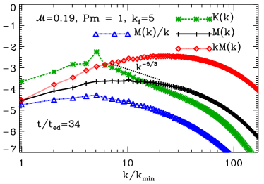
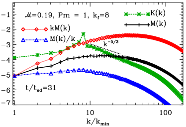
Figure 1: Power spectra of kinetic energy, $K(k)$ (green dashed); magnetic energy, $M(k)$ (black, solid); $k\,M(k)$ (red, dotted); and $M(k)/k$ (blue, dash-dotted) for run B (left) and run C (right). These spectra are computed from a snapshot in the saturated state for the respective runs. The black dotted line shows the $k^{-5/3}$ for comparison. Here, the wave number is normalized in units of $k_{\rm min}=2\pi/L$.

In this section, we use the synthetic observations to investigate the statistical properties of the polarized emission from the diffuse ICM. In Sur et al. (2021), it was shown that the power spectrum computed from the 2-D map of Faraday depth (FD), the line of sight integral of $B_{\|}$ weighted by $n_{\rm e}$, could be directly used to infer the magnetic integral scale, i.e., the coherence scale of the magnetic fields, in the ICM also see (Cho and Ryu, 2009), provided FD is measured accurately. It was also found that, for turbulence driven on 256 kpc, broad-bandwidth spectro-polarimetric observations $\gtrsim$3  GHz are well suited for detecting and inferring the intrinsic polarization properties of the ICM, and the polarized emission could be well recovered by applying the technique of rotation measure (RM) synthesis (Brentjens and de Bruyn, 2005; Heald et al., 2009). Here, we will focus on the statistical properties of the total and polarized synchrotron emission from the ICM for turbulence driven on different scales and the impact of smoothing the emission by a telescope beam. It will become clear from the following sections, the different scales of turbulent driving adopted in this work allow us to probe the effects of magnetic fields with varying correlation scales on the statistical nature of the polarized emission.

Before we focus our attention on the different correlation scales, we show in Figure 1, the 1-D power spectra of the kinetic energy $K(k)$ (green dashed with asterisks); magnetic energy, $M(k)$ (black, solid line with plus symbols); spectra of $k\,M(k)$ (red, dotted line with diamonds) representing the largest energy-carrying scale of the field; and that of $M(k)/k$ (blue, dash-dotted line with triangles), which provides an estimate of the magnetic integral scale. Here, $k$ is the wave number. These spectra are obtained from snapshots in the non-linear saturated state of the dynamo when turbulence is forced at $k_{\rm f}=5$ (left-hand panel) and $k_{\rm f}=8$ (right-hand panel). The corresponding plot for $k_{\rm f}=2$ can be gleaned from Figure 1 of Sur et al. (2021). The peak of $M(k)$ lies at $\approx$1/10 of the box size for $k_{\rm f}=5$ and at $\approx$1/20 for $k_{\rm f}=8$. On the other hand, the peak of $k\,M(k)$ occurs at much smaller scales compared to the respective forcing scales in both cases. The peak of $M(k)/k$ occurs on a scale very close to the turbulent driving scale in both cases. These findings are qualitatively similar to the ones obtained in Sur et al. (2021) when turbulence is forced at $k_{\rm f}=2$.

We find that, although turbulence is driven on different scales, the dispersion of Faraday depth ($\sigma_{\rm FD}$) are similar in all the cases having value $\sigma_{\rm FD}\sim 100\,{\rm rad\,m^{-2}}$. For $k_{\rm f}=2$, FD lies in the range $-438$ to $+415\,{\rm rad\,m^{-2}}$ with $\sigma_{\rm FD}\approx 118\,{\rm rad\,m^{-2}}$; for $k_{\rm f}=5$, FD ranges between $-505$ and $+443\,{\rm rad\,m^{-2}}$ with $\sigma_{\rm FD}\approx 103\,{\rm rad\,m^{-2}}$; and for $k_{\rm f}=8$, FD lies in the range $-552$ to $430\,{\rm rad\,m^{-2}}$ having $\sigma_{\rm FD}\approx 93\,{\rm rad\,m^{-2}}$. There is a mild indication that $\sigma_{\rm FD}$ decreases with decreasing turbulence forcing scale ${l_{\rm f}}$. This is because, $\sigma_{\rm FD}$ depends on the magnetic integral scale see Equation (2) in (Sur et al., 2021), which, as we will discuss in the following sections, decreases with ${l_{\rm f}}$. Even though $\sigma_{\rm FD}$ decreases, beam and frequency-dependent Faraday depolarization are stronger for smaller forcing scales caused by the smaller scale filamentary magnetic field structures generated by the action of fluctuation dynamo. A quantitative investigation on the properties of frequency-dependent Faraday depolarization and their dependence on turbulence driving scale will be presented elsewhere.

For completeness, in Figure 2, we show the power spectra of the map of FD in the kinematic and saturated stage of the dynamo for ${l_{\rm f}}=102.4\,{\rm kpc}$ (left-hand panel) and $64\,{\rm kpc}$ (right-hand panel). For comparison, we also show the power spectra of $M(k)/k$ with dotted lines. As found for ${l_{\rm f}}=256\,{\rm kpc}$ in Sur et al. (2021), we find excellent match between the power spectra of FD and the corresponding $M(k)/k$ for all the cases, indicating that power spectrum of FD maps can provide valuable insight into the magnetic correlation scale in the ICM. However, as demonstrated in Sur et al. (2021), estimating FD map from observations is challenging due to the limitations of available techniques, such as, the technique of RM synthesis. However, RM synthesis can recover the fractional polarization $p$ well, especially from broad-bandwidth spectro-polarimetric observations $\gtrsim$3  GHz. Therefore, in the following, we will investigate the information on magnetic field properties that can be extracted from $p$.

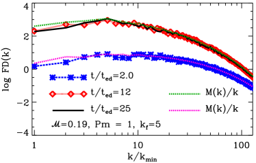
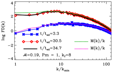
Figure 2: Power spectra of the Faraday depth. The blue dotted curve corresponds to the spectra in the kinematic phase, while the red dashed and black curves correspond the spectra in the saturated phase at two different times. For comparison, the magenta and green dashed curves show the scaled spectra of $M(k)/k$ in the kinematic and saturated phases, respectively. The left and right figures correspond to $k_{\rm f}=5$ and $k_{\rm f}=8$ simulations, respectively. Here, the wave number is normalized in units of $k_{\rm min}=2\pi/L$.

3.1 Correlation Scales in the ICM

The ICM can be characterized in terms of a number of distinct scales. Since we are primarily concerned with the effects of turbulence in this work, it is therefore important that the integral scales of the turbulent velocity and random magnetic fields be compared with the integral scales of the relevant observables, such as the FD, the total synchrotron intensity (${I_{\rm sync}}$) and the polarized intensity (${\rm PI}$). While these scales may be difficult to estimate directly from observations of the ICM, it can be easily derived from our simulations thereby providing a first hand estimate which may be confirmed with suitable future observations. For example, the integral scales of the turbulent velocity ($L_{{\rm int},V}$) and random magnetic fields ($L_{{\rm int},M}$) can be obtained from their respective power spectra as,

$$L_{{\rm int},V}=\frac{2\pi\int[K(k)/k]\,dk}{\int K(k)\,dk},\,\,\,\,\,L_{{\rm int},M}=\frac{2\pi\int[M(k)/k]\,dk}{\int M(k)\,dk}.$$ (1)

Estimates of the integral scales of FD, ${I_{\rm sync}}$ and ${\rm PI}$ can similarly be obtained from Equation (1) by using the appropriate power spectrum corresponding to the observable.

Table 3 lists the integral scales across different forcing scales computed directly from the simulations and the synthetic observations. In order to estimate the sensitivity of these scales to the random fluctuations in the field, the values of the integral scales are shown at two different times selected from the non-linear saturated state of the system in each case. Irrespective of the forcing scale of turbulence, we find that the velocity integral scale $L_{{\rm int},V}\approx 2.2\textrm{--}3\,L_{{\rm int},M}$, in agreement with the estimates obtained for subsonic tubulence in earlier studies (Bhat and Subramanian, 2013; Sur et al., 2018). We further find that, despite random scatter from one realization to another, the integral scales associated with the observables, FD, $I_{\rm sync}$ and ${\rm PI}$ are all larger than $L_{{\rm int},M}$ by a factor $\sim$2–2.5, depending on the forcing scale ($l_{\rm f}$). The integral scale of $I_{\rm sync}$ in each case, appears to be somewhat larger than $L_{\rm int,FD}$ and $L_{\rm int,PI}$ at frequencies $\gtrsim$4  GHz. Glimpses of the effects of Faraday depolarization is evident from the estimates of $L_{\rm int,PI}$ at lower frequencies, wherein, $L_{\rm int,PI}$ at $\nu<1.4~{}\,{\rm GHz}$ are generally smaller compared to the ones at $\nu=5~{}\,{\rm GHz}$ due to small-scale structures introduced by Faraday depolarization.

Table 3: Values of the integral scales (in kpc) of the velocity ($L_{{\rm int},V}$), magnetic fields ($L_{{\rm int},M}$), Faraday depth ($L_{\rm int,FD}$), the total synchrotron intensity ($L_{{\rm int},I}$) at $1~{}\,{\rm GHz}$, and, the polarized intensity ($L_{{\rm int},{PI}}$) at $0.6$, $1.2$ and $5~{}\,{\rm GHz}$ at two different times in the steady state obtained from three simulations where turbulence is driven on scales of $l_{\rm f}=256,102.4$ and $64~{}\,{\rm kpc}.$

$k_{\rm f}$	$t/t_{\rm ed}$	$L_{{\rm int},V}$	$L_{{\rm int},M}$	$L_{\rm int,FD}$	$L_{{\rm int},I}$	$L_{\rm int,PI}~{}(\,{\rm kpc})$
(Forcing Scale)		$(\,{\rm kpc})$	$(\,{\rm kpc})$	$(\,{\rm kpc})$	$(\,{\rm kpc})$	$0.6\,{\rm GHz}$	$1.2\,{\rm GHz}$	$5\,{\rm GHz}$
2	16.6	320	106	212.5	224	125.5	157.5	194
(256 kpc)	23	340	112.4	216	227.6	140	159	188
5	20.2	98.7	40.7	78.8	130	57.3	55.0	88.6
(102.4 kpc)	24.5	99.1	40.8	87.5	120.2	57.7	60.3	87.0
8	30.6	62.4	27.6	58.0	86.0	38.3	37.1	70.2
(64 kpc)	34.7	62.4	28.0	61.6	89.5	35.0	34.0	74.2

3.2 Smoothing of Total Intensity

$l_{\rm f}=256\,{\rm kpc}$	$l_{\rm f}=102.4\,{\rm kpc}$	$l_{\rm f}=64\,{\rm kpc}$

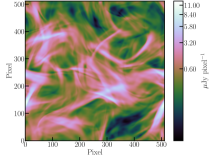
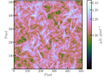
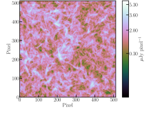
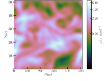
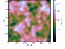
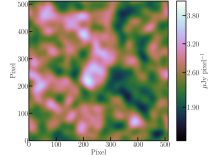
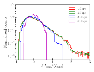
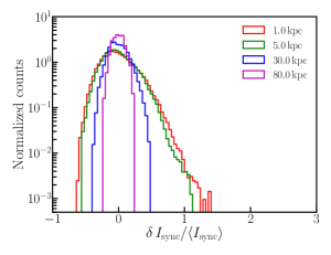
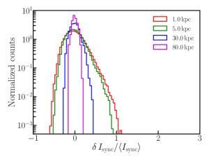
Figure 3: Top row: The 2-D maps of surface brightness of the total synchrotron emission ($I_{\rm sync}$) at the native 1 kpc resolution of the simulations. Middle row: Synchrotron total intensity maps in the top row smoothed by a Gaussian kernel with $\rm FWHM=30\,{\rm kpc}$. Bottom row: Pixel-wise distribution of $\delta\,{I_{\rm sync}}/\langle{I_{\rm sync}}\rangle$ for smoothing the total synchrotron intensity on different scales shown with different colours. The Left, middle and right columns are for synthetic observations of $l_{\rm f}=256\,{\rm kpc}$ at $t/t_{\rm ed}=23$, $l_{\rm f}=102.4\,{\rm kpc}$ at $t/t_{\rm ed}=20.2$, and $l_{\rm f}=64\,{\rm kpc}$ at $t/t_{\rm ed}=30.6$, respectively.

For our assumed constant spatial distribution of $n_{\rm CRE}$ in each mesh point, the synchrotron intensity ($I_{\rm sync}$) in the plane of the sky is directly dependent on $B_{\perp}$ as $I_{\rm sync}\propto\int\,B_{\perp}^{1-\alpha}\,dl$. Hence, the filamentary magnetic field structures generated due to the action of fluctuation dynamo are also observed in the synthetic synchrotron intensity map. These structures, along with non-linear dependence of the $I_{\rm sync}$ on $B_{\perp}$, gives rise to a log-normal distribution of the $I_{\rm sync}$ with long tails when observed with resolution comparable to that of the simulations also see (Sur et al., 2021). In the top row of Figure 3 we show the maps of ${I_{\rm sync}}$, where, the left, the middle and the right columns are for forcing at 256, 102.4 and 64 kpc. It is clearly seen that when turbulence is forced on smaller scales, the filamentary structures in ${I_{\rm sync}}$ become more volume filling. These filaments have smaller extent for smaller ${l_{\rm f}}$, which is also evident from the integral scale of the synchrotron emission ($L_{{\rm int},I}$) given in Table 3, and seen in Figure 4 (right). In the absence of shocks (due to subsonic turbulence) these filamentary structures are a direct signature of fluctuation dynamos in the ICM. We find that both $L_{{\rm int},I}$ and $L_{{\rm int},M}$ increases linearly with $l_{\rm f}$, except that $L_{{\rm int},I}$ is higher than $L_{{\rm int},M}$ by roughly a factor of 2. Furthermore, the intensity contrast decreases significantly when turbulence is forced on smaller scales. The middle row of Figure 3 shows the total intensity maps in top row smoothed on 30 kpc (FWHM). It is clear that observations with a telescope smears the filamentary features and significantly reduces the intensity contrast.

Interestingly, radio continuum observations reveal that the emission from halos of galaxy clusters are spatially smooth (Cuciti et al., 2021), devoid of the filamentary structures seen at the native resolution of the simulations. Hence, it is important to assess the extent to which telescope beams smear out such structures, and whether they can be discerned with respect to the diffuse background emission. In the bottom row of Figure 3, we show the pixel-wise distribution of overdensity of $I_{\rm sync}$, i.e., $\delta\,I_{\rm sync}/\langle I_{\rm sync}\rangle$ at the native 1 kpc resolution of the simulations and for smoothing over different spatial scales mimicking astronomical observations performed with different telescopes resolutions. Here, $\langle I_{\rm sync}\rangle$ is the mean $I_{\rm sync}$ over the map, and $\delta\,{I_{\rm sync}}={I_{\rm sync}}-\langle{I_{\rm sync}}\rangle$. The bright filamentary structures with $\delta\,{I_{\rm sync}}/\langle{I_{\rm sync}}\rangle>1$ are clearly seen as long tails of the distribution at 1 kpc resolution and for smoothing on 5 kpc scales when turbulence is forced on 256 kpc scale. However, for forcing on 102.4 and 64 kpc scales, the maximum overdensity decreases significantly to $\sim$1. In fact, the Fisher-Pearson coefficient of skewness ($g_{1}$) of the distributions decreases from 1.4 for forcing on 256 kpc scale to 0.62 for forcing on 102.4 and 64 kpc scales, indicating that the distribution of surface brightness of the synchrotron emission for turbulence driving on scales $\lesssim$100  kpc to be relatively symmetrical. This is due to the fact that, the filamentary structures are more volume filling when turbulence is driven on smaller scales. These results suggest that, in the presence of realistic telescope noise, coupled with generically low surface brightness, the filamentary structures in total intensity emission from the radio halos of galaxy clusters would be difficult to discern even when observed with relatively high spatial resolutions of $\sim$10–20  kpc.

Smoothing the synthetic ${I_{\rm sync}}$ maps on larger spatial scales of 30 and 80 kpc, which are the typical spatial resolutions achieved with existing observations of radio halos, we find that $\delta\,{I_{\rm sync}}/\langle{I_{\rm sync}}\rangle$ decreases significantly below 1 in almost every pixel, making the distributions symmetric with $g_{1}<0.2$ for all the three scales of turbulence driving. The situation is expected to be further aggravated in the presence of telescope noise and demonstrates why such filamentary structures seen in the simulations have not been observed. In order to detect the fluctuations in ${I_{\rm sync}}$, sensitive, high resolution observations ($<$5  kpc) are of paramount importance. It is noteworthy, in contrast to the nearly uniform $n_{\rm e}$ (fluctuations in overdensity are at $3\%$ level for $\mathcal{M}\approx$ 0.18–0.19) and uniform distribution of $n_{\rm CRE}$ assumed in our models for the core region in ICM, the magnetic field strength, $n_{\rm e}$ and $n_{\rm CRE}$ are likely to be stratified in galaxy clusters, decreasing away from the cluster core on scales of hundreds of kpc over the entire volume. Hence, stratification of these physical quantities could give rise to skewness in the distribution of the synchrotron surface brightness even if observed using significantly smoothed beam.

3.3 Intrinsic Polarization and Forcing Scale

Although, results from numerical simulations of fluctuation dynamos in the ICM suggest that cluster halos are expected to be intrinsically polarized at 10–30% level (Sur et al., 2021), unambiguous detection of polarized emission remains elusive. Work by Govoni and Feretti (2004) found cluster radio halos to be polarized with $p<2\textrm{--}10\%$ at $1.4\,{\rm GHz}$. Thierbach et al. (2003) failed to detect any significant diffuse polarized emission in the Coma cluster at 2.67 and $4.85~{}\,{\rm GHz}$ with linear resolutions of $110$ and $60\,{\rm kpc}$, respectively. This could be due to a combination of Faraday and beam depolarization, and insufficient sensitivity. In light of these results, we present here the statistical properties of the polarized synchrotron emission when smoothed on different scales by a telescope beam. Before delving into them in detail, we first discuss the intrinsic properties of the fractional polarization ($p_{\rm int}$) at the native 1 kpc resolution of the simulations, and in the absence of frequency-dependent Faraday depolarization (equivalent to $p$ at wavelength $\lambda=0$).

In the presence of random magnetic fields, polarized emission originating at different depths in the ICM is expected to undergo random walk as the LOS passes through a number of magnetic cells, within which the field is ordered but, randomly oriented from cell to cell. This leads to rotation of the plane of polarization by random angles resulting in a random degree of polarization. Therefore, the volume-averaged intrinsic fractional polarization (${\langle p\rangle}_{\rm int}$) is expected to depend as ${\langle p\rangle}_{\rm int}\approx p_{\rm max}/\sqrt{N_{\rm mag}}$ (Sokoloff et al., 1998). Here, $p_{\rm max}=(1-\alpha)/(5/3-\alpha)=0.75$ (for $\alpha=-1$) is the maximum fractional polarization and, $N_{\rm mag}=L/L_{{\rm int},M}$ is the number of magnetic cells along the LOS. The above relation hints to a decrease of ${\langle p\rangle}_{\rm int}$ with decreasing $l_{\rm f}$. This can be intuitively understood from the fact that a smaller $l_{\rm f}$ implies a larger value of $N_{\rm mag}$ as $L_{{\rm int},M}<l_{\rm f}<L$. In fact, Table 3 shows that $L_{{\rm int},M}$ is smaller by a factor of $\approx$4 in each dimension for $l_{\rm f}=64\,{\rm kpc}$, compared to $l_{\rm f}=256\,{\rm kpc}$. This translates to $N_{\rm mag}$ being larger by the same factor for $l_{\rm f}=64\,{\rm kpc}$, which would result in a larger cancellation of the polarized emission along the LOS, and hence, lower ${\langle p\rangle}_{\rm int}$.

In order to understand how ${\langle p\rangle}_{\rm int}$ changes with the driving scale $l_{\rm f}$ due to different number of magnetic correlation scales within the volume, we computed the fractional polarization by turning off the effects of Faraday rotation when generating the synthetic observations. Note that, in the absence of Faraday rotation, $p$ is independent of $\nu$. In Table 4, we list the frequency-independent ${\langle p\rangle}_{\rm int}$ and its dispersion computed from the maps of $p_{\rm int}$ for different ${l_{\rm f}}$. The values of ${\langle p\rangle}_{\rm int}=\langle{\rm PI}/I\rangle$ computed from the maps of polarized intensity and the total synchrotron intensity are also depicted by black points in the left-hand panel of Figure 4. In the same figure, we also show, for comparison, the expected ${\langle p\rangle}_{\rm int}$, computed as ${\langle p\rangle}=p_{\rm max}/\sqrt{N_{\rm mag}}$ by using $L_{{\rm int},M}$ from Table 3, as the grey points. The variation of ${\langle p\rangle}_{\rm int}$ with $l_{\rm f}$, computed directly from the synthetic maps and from expectation, remarkably follows the ${\langle p\rangle}\propto l_{\rm f}^{1/2}$ relation, shown as the blue curve in Figure 4 (left). Such a relation is expected for Gaussian random magnetic fields, and finding this relation for intermittent magnetic fields generated by the fluctuation dynamo indicates that the polarization vector undergo random walk similar to Gaussian random fields when the LOS is integrated over several magnetic integral scales. To our knowledge, this is the first time we confirm such a relation for fluctuation dynamo-generated intermittent magnetic fields.

Table 4: Values of ${\langle p\rangle}$ and $\sigma_{p}$ obtained from the synthetic maps at 5, 1.2 and 0.6 GHz for the three forcing scales ${l_{\rm f}}=256,102.4$ and $64\,{\rm kpc}$. The ‘intrinsic’ values refers to the frequency-independent values, equivalent at $\lambda=0$, obtained by turning off the effects of Faraday rotation. $p_{0}$ and $l_{1/2}$ are the best-fit values obtained by fitting the variation of ${\langle p\rangle}$ with smoothing scale modelled by Equation (2).

Forcing Scale	Frequency	$\langle p\rangle,\sigma_{p}$	$p_{0}$	$l_{1/2}$
(kpc)	(GHz)			(kpc)
256	Intrinsic	$0.35,0.13$	$0.356\pm 0.004$	$197.0\pm 14.9$
	5.0	$0.34,0.13$	$0.352\pm 0.003$	$155.1\pm 7.8$
	1.2	$0.20,0.10$	$0.20\pm 0.01$	$9.3\pm 1.0$
	0.6	$0.11,0.07$	$0.14\pm 0.04$	$2.1\pm 0.6$
102.4	Intrinsic	$0.20,0.10$	$0.22\pm 0.01$	$36.2\pm 4.0$
	5.0	$0.20,0.10$	$0.22\pm 0.01$	$33.3\pm 2.9$
	1.2	$0.16,0.08$	$0.15\pm 0.03$	$4.7\pm 1.2$
	0.6	$0.10,0.06$	$0.20\pm 0.11$	$0.8\pm 0.5$
64	Intrinsic	$0.17,0.09$	$0.20\pm 0.01$	$22.8\pm 2.4$
	5.0	$0.17,0.09$	$0.19\pm 0.01$	$21.5\pm 1.9$
	1.2	$0.14,0.07$	$0.17\pm 0.04$	$2.5\pm 0.6$
	0.6	$0.09,0.05$	$0.80\pm 0.80$	$0.12\pm 0.12$

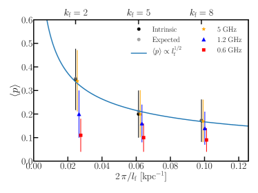
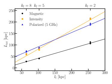
Figure 4: Left: Variation of mean fractional polarization $\langle p\rangle$ with the turbulence driving scale $l_{\rm f}$ in the saturated stage at the native resolution of the simulations. The black points show the intrinsic ${\langle p\rangle}$ from the simulated volumes computed in the absence of Faraday rotation. The grey points show the expected ${\langle p\rangle}$ computed from the magnetic integral scale. The blue curve shows $\langle p\rangle\propto l_{\rm f}^{1/2}$ variation. The red squares, blue triangles and orange stars correspond to 0.6, 1.2 and 5 GHz in the presence of Faraday rotation, and they are plotted with slight offset to avoid overlap. All errors show the standard deviation of pixels in the fractional polarization maps. Right: Variation of the integral scales with $l_{\rm f}$. The black, orange and blue points are for the magnetic field, total intensity and polarized intensity at 5 GHz, respectively. The lines shows $L_{\rm int}\propto l_{\rm f}$.

The fact that ${\langle p\rangle}_{\rm int}$ varies as $l_{\rm f}^{1/2}$, indicates a possible linear relationship between $l_{\rm f}$ and $L_{{\rm int},M}$. This is indeed seen in our simulations and is shown in the right-hand panel of Figure 4. Here, we plot the variation of the integral scales of magnetic field (in black) and synchrotron intensity (in orange), $L_{{\rm int},M}$ and $L_{{\rm int},I}$, respectively, as a function of $l_{\rm f}$. This linear dependence of $L_{{\rm int},M}$ on $l_{\rm f}$ suggests that ${\langle p\rangle}_{\rm int}$ of the ICM is a direct indicator of the forcing and/or magnetic integral scale.

In the following, we investigate how frequency-dependent Faraday depolarization affect the variation of ${\langle p\rangle}$ with ${l_{\rm f}}$. Details of numerical computations of the frequency-dependent Faraday depolarization is presented in Basu et al. (2019) and Sur et al. (2021). In the left-hand panel of Figure 4, we also show variation of ${\langle p\rangle}$ with ${l_{\rm f}}$ determined from the synthetic maps in the presence of Faraday rotation at 5, 1.2 and 0.6 GHz with orange stars, blue triangles and red squares, respectively. The values of ${\langle p\rangle}$ and its pixel-wise dispersion $\sigma_{p}$ obtained at the native resolution of 1 kpc at these frequencies are listed in Table 4. It is immediately evident that, due to relatively low Faraday depolarization at 5 GHz, the variation of ${\langle p\rangle}_{\rm 5\,GHz}$ with ${l_{\rm f}}$ matches excellently with that of ${\langle p\rangle}_{\rm int}$ and dropping by a factor of two as $l_{\rm f}$ decreases from $256$ to $64\,{\rm kpc}$. This emphasizes the fact that measurement of polarized emission from the ICM at frequencies $\gtrsim$4  GHz, where Faraday rotation is low, can be directly used to gain insights into the nature of turbulence driving in the ICM of galaxy clusters. At lower frequencies, ${\langle p\rangle}_{\rm 1.2\,{\rm GHz}}$ and ${\langle p\rangle}_{\rm 0.6\,{\rm GHz}}$ change mildly with ${l_{\rm f}}$ (see Table 4), deviating significantly from the ${l_{\rm f}}^{1/2}$ dependence. Furthermore, as mentioned earlier, the dispersion of Faraday depth, $\sigma_{\rm FD}$, for all the three forcing scales are similar with $\sigma_{\rm FD}\approx 100\,{\rm rad\,m^{-2}}$. That means, small-scale structures introduced due to strong Faraday depolarization at frequencies $\lesssim$3  GHz see (Sur et al., 2021) makes ${\langle p\rangle}$ insensitive to $L_{{\rm int},M}$. Therefore, even if polarized emission from the diffuse ICM at frequencies $\lesssim$3  GHz are detected, they will be unsuitable to glean any meaningful insight into the magnetic field properties.

3.4 Smoothing of Polarization Parameters

In the previous subsection, we demonstrated that the observed ${\langle p\rangle}$ of the ICM measured at frequencies $\gtrsim$4  GHz directly provides an estimate of the turbulent forcing scale when observations are performed with spatial resolution comparable to or higher than the 1 kpc resolution of the simulations. However, achieving such resolutions is challenging with currently available radio telescopes. Here, we consider the statistical properties of ${\langle p\rangle}$ measured at different frequencies smoothed on various scales in the presence of frequency-dependent Faraday depolarization. In the top-panel of Figure 5, we show the pixel-wise empirical cumulative distribution function (CDF) of $p$ smoothed on various scales at 5, 1.2 and 0.6 GHz for ${l_{\rm f}}=256\,{\rm kpc}$. The CDFs for ${l_{\rm f}}=102.4$ and $64\,{\rm kpc}$ are shown in Figures 7 and 8, respectively. From the top-row of Figure 5 it is evident that the CDFs shift towards the left with increasing smoothing scale, indicating ${\langle p\rangle}_{\nu}$ decreases with smoothing on larger scales due to a combination of beam and Faraday depolarization. At 5 GHz, ${\langle p\rangle}_{5\,{\rm GHz}}$ decreases by about 30% from 0.35 at the native resolution to 0.25 when smoothed on 80 kpc scales for ${l_{\rm f}}=256\,{\rm kpc}$. However, as a consequence of stronger Faraday depolarization at lower frequencies, the decrease in ${\langle p\rangle}_{\nu}$ with smoothing scale is stronger, wherein ${\langle p\rangle}_{1.2\,{\rm GHz}}$ decreases from 0.2 at native resolution to significantly below 0.05 for smoothing on 80 kpc, and at 0.6 GHz, ${\langle p\rangle}_{0.6\,{\rm GHz}}$ decreases from 0.11 to about 0.01. For lower ${l_{\rm f}}$ of 102.4 and 64 kpc, in general we find that, due to larger $N_{\rm mag}$ (see Secion 3.3), the rate of decrease of ${\langle p\rangle}_{\nu}$ with increasing smoothing scale is significantly larger compared to ${l_{\rm f}}=256\,{\rm kpc}$ at all the three frequencies.

5 GHz	1.2 GHz	0.6 GHz

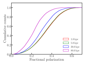
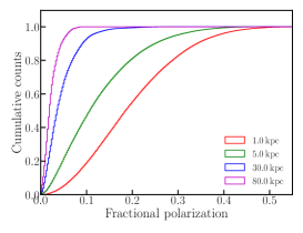
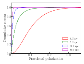
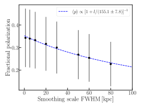
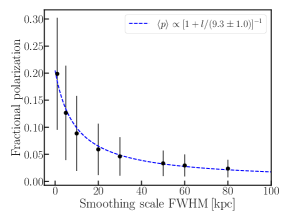
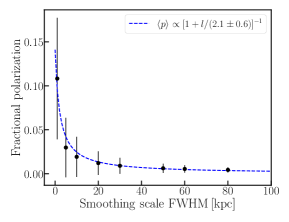
Figure 5: Effect of smoothing by different scales on the fractional polarization ($p$) obtained from ${l_{\rm f}}=256$ kpc at $t/t_{\rm ed}=23$. Top panel: Cumulative distribution of $p$ for smoothing by different scales. Bottom panel: Variation of the mean fractional polarization $\langle p\rangle$ as a function of the smoothing scale ($l$). The dashed blue curve show the best-fit to the points using Equation (2). Left, middle and right rows are for synthetic observations at 5, 1.2 and 0.6 GHz, respectively.

We model the depolarization as a function of smoothing scale in the presence of Faraday rotation seen in the top panel of Figure 5 using the form,

$$\langle p(l)\rangle={p_{0}}\,{\left(\frac{1}{1+l/l_{1/2}}\right)}.$$ (2)

Here, $l$ is the spatial smoothing scale, $p_{0}$ provides estimate of $\langle p\rangle$ at infinitesimal resolution, and $l_{1/2}$ is the smoothing scale at which the mean fractional polarization decreases by 50%, i.e., $\langle p(l_{1/2})\rangle=p_{0}/2$. In the bottom panel of Figure 5, we show the variation of ${\langle p\rangle}_{\nu}$ for ${l_{\rm f}}=256\,{\rm kpc}$ as the data points, and the best-fit model using Equation (2). The corresponding plots for ${l_{\rm f}}=102.4$ and $64\,{\rm kpc}$ are shown in the bottom panels of Figures 7 and 8, respectively. The best-fit parameters, $p_{0}$ and $l_{1/2}$, for all the three ${l_{\rm f}}$ at the three representative frequencies and for ${\langle p\rangle}_{\rm int}$ are presented in Table 4. Firstly we note that, for the frequency-independent ${\langle p\rangle}_{\rm int}$, $l_{1/2}$ reduces drastically from $\approx$200  kpc for ${l_{\rm f}}=256\,{\rm kpc}$ to $l_{1/2}\approx 20\,{\rm kpc}$ for ${l_{\rm f}}=64\,{\rm kpc}$. This decrease in $l_{1/2}$ with ${l_{\rm f}}$ is significantly non-linear, in contrast to what was found in the right-hand panel of Figure 4 for the different integral scales, and could be qualitatively understood as a consequence of increasing variance of the random magnetic fields within the beam for lower ${l_{\rm f}}$ see, e.g., (Sokoloff et al., 1998). Therefore, we believe that it is difficult to use $l_{1/2}$ as an indicator of ${l_{\rm f}}$ in a straightforward way. Secondly, in the presence of frequency-dependent Faraday depolarization, for a given ${l_{\rm f}}$, $l_{1/2}$ becomes drastically smaller at lower frequencies. For example, when turbulence is driven on $256\,{\rm kpc}$, $l_{1/2}$ decreases from $155.1\pm 7.8\,{\rm kpc}$ at $5\,{\rm GHz}$ to only $2.1\pm 0.6\,{\rm kpc}$, comparable to the resolution of the simulations, at $0.6\,{\rm GHz}$. Thirdly, the decrease in $l_{1/2}$ with decreasing frequency is significantly stronger for smaller ${l_{\rm f}}$, so that $l_{1/2}$ becomes comparable to, or smaller than, the resolution of the simulations for ${l_{\rm f}}\lesssim 100\,{\rm kpc}$ at frequencies $\lesssim$1  GHz (see Table 4). Our findings imply that due to the small-scale structures introduced by the effect of Faraday depolarization, beam depolarization completely wipes out the intrinsic polarized structures. This reduces the level of polarization from the ICM to insignificant levels at frequencies below $1\,{\rm GHz}$, even if observations are performed with high spatial resolutions of $\sim$1–5  kpc. This re-emphasizes the finding in Sur et al. (2021) that, high frequency observations $\gtrsim$3  GHz with high spatial resolutions $\lesssim$20  kpc are of paramount importance in order to detect diffuse polarized emission from the radio halo of galaxy clusters.

4 Discussion and Conclusions

In this paper, we presented detailed investigation of the expected statistical properties of polarized emission from the ICM of galaxy clusters for different scales of turbulent driving of fluctuation dynamo, and the effect of beam smoothing when observations are performed using a finite telescope resolution. To obtain synthetic observations, covering the frequency range 0.6 to 5 GHz, we made use of three non-ideal MHD simulations of fluctuation dynamos with turbulence driven on 256, 102.4 and 64 kpc scales. The resultant rms Mach numbers in these simulations are in the range $\mathcal{M}=0.18\textrm{--}0.19$. Thus, in the absence of any noticeable density fluctuations, these simulations allowed us to probe the effects of magnetic fields on the properties of the polarized emission. The simulations were performed over $512\,{\rm kpc}^{3}$ volume with a resolution of $1\,{\rm kpc}$ along each axes. The 2-D maps of various observables have spatial size of $512\times 512\,{\rm kpc}^{2}$ in the plane of the sky with each pixel separated by 1 kpc. For the purpose of studying the impact of a telescope beam on the level of polarization in the ICM, we have smoothed the synthetic maps on various scales ranging between 5 and 80 kpc.

Fluctuation dynamo generates highly non-Gaussian, spatially intermittent distribution of the magnetic field components giving rise to filamentary structures in the synchrotron total intensity maps that are extended roughly on scales of turbulence driving (see Table 3). These filaments give rise to long tails in the surface brightness distribution of the synchrotron emission as presented in Section 3.2. However, these structures are significantly smeared-out when smoothed on scales $\gtrsim$30  kpc, especially for the smaller turbulence driving scales ${l_{\rm f}}\lesssim 100\,{\rm kpc}$ where the filamentary structures are more volume filling and thereby results in lower intensity contrast. Our work shows that, in the presence of realistic noise and due to the faint surface brightness of the diffuse synchrotron emission from the ICM, such filamentary structures are difficult to discern in current observations.

In Section 3.3, we show for the first time that in the presence of spatially intermittent magnetic fields the mean intrinsic fractional polarization ${\langle p\rangle}_{\rm int}$ at 1 kpc resolution of the simulations varies with the turbulence driving scale ${l_{\rm f}}$ as ${\langle p\rangle}_{\rm int}\propto{l_{\rm f}}^{1/2}$. This implies that ${\langle p\rangle}_{\rm int}$ when estimated at $\lambda=0$ using the technique of Stokes $Q,U$ fitting (O’Sullivan et al., 2012, 2015) applied to broad-bandwidth spectro-polarimetric observations of radio halos could be used to directly infer the correlation scale of the magnetic fields in the ICM. However, due to the extremely faint surface brightness of the polarized emission which is expected to be of the order of a fraction of $\mu$Jy arcsec^-2, applying Stokes $Q,U$ fitting would be a challenging proposition. This limitation can be easily circumvented by performing polarization observation at frequencies $\gtrsim$4  GHz. As shown in Figure 4, due to significantly low Faraday depolarization, ${\langle p\rangle}$ can be confidently used to infer the magnetic correlation scales in the ICM, provided observations are performed with sufficiently high spatial resolution. This is evident from Figure 6 where we compare the variation of the mean fractional polarization at 5 GHz, ${\langle p\rangle}_{5\,{\rm GHz}}$, versus $l_{\rm f}$ at the native resolution of the simulations, with those obtained by smoothing on different scales. It is clear from the plot that even at high frequencies ($\nu>4\,{\rm GHz}$), ${\langle p\rangle}_{5\,{\rm GHz}}$ deviates significantly from $\propto l_{\rm f}^{1/2}$ relation when the maps are smoothed to a resolution of $30\,{\rm kpc}$, especially for ${l_{\rm f}}<100\,{\rm kpc}$. On the other hand, at frequencies $\lesssim$2  GHz, Faraday depolarization gives rise to small-scale structures in the observed Stokes $Q$ and $U$ maps. Therefore, even if polarized emission from radio halos are detected at these frequencies, they would be of limited use for inferring about the intrinsic properties of the magnetic fields in the ICM.

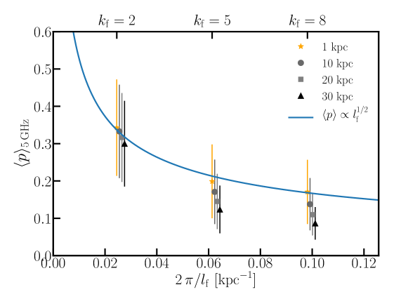
Figure 6: Variation of the mean fractional polarization at 5 GHz, ${\langle p\rangle}_{5\,{\rm GHz}}$, with the turbulence driving scale $l_{\rm f}$ in the saturated stage. The different coloured symbols are ${\langle p\rangle}$ obtained by smoothing on different scales. The blue curve shows the ${\langle p\rangle}\propto l_{\rm f}^{1/2}$ variation, same as in Figure 4 (left-hand panel).

The expected ${\langle p\rangle}$ in the ICM is significantly reduced due to a combination of frequency-dependent Faraday depolarization and when observations are smoothed by a telescope beam (see, e.g., Figure 6). In general, reduction of ${\langle p\rangle}$ due to beam smoothing is stronger for turbulence driven on smaller scales. In Section 3.4, we find that at frequencies $\lesssim$3  GHz, ${\langle p\rangle}$ reduces by more than 50% when smoothed on about $10\,{\rm kpc}$ scales for turbulent driving on any of the three scales investigated in this study. In fact, at low frequencies, smoothing the emission from the ICM on about 30 kpc scales reduces ${\langle p\rangle}$ by more than a factor of five, making the detection of diffuse polarized emission challenging. However, pockets of clumpy emission, extended on scales of a few beam, could be substantially polarized up to about 10–20% level. Detection of such features at low frequencies would contain limited information on the nature of the magnetic fields also see (Sur et al., 2021). At frequencies $\gtrsim$4  GHz, the diffuse polarized emission from the ICM is largely unaffected by Faraday depolarization, and ${\langle p\rangle}$ is only mildly reduced for turbulence driven on larger scales $\gtrsim$100  kpc. For turbulence driven on scales below $\sim$100  kpc, ${\langle p\rangle}$ of the diffuse ICM reduces to half when the emission is smoothed on scales $>$20  kpc. That means, the level of polarized emission from the ICM when observed with resolutions better than 6 arcsec at frequencies $>$4  GHz for galaxy clusters located up to redshift $z=0.2$ contains valuable information on the turbulence driving scale.

Our results on the effect of beam smoothing on the expected mean fractional polarization ${\langle p\rangle}$ for different driving scale of turbulence, in combination with the ${\langle p\rangle}\propto{l_{\rm f}}^{1/2}$ relation, brings to light an important fact that ${\langle p\rangle}$ measured at frequencies above $4\,{\rm GHz}$ can be used to glean information on ${l_{\rm f}}$. It is clear from Figure 6 that ${\langle p\rangle}_{5\,{\rm GHz}}$ is relatively less affected by smoothing for large ${l_{\rm f}}$. This implies, detection of diffuse polarized emission near $5\,{\rm GHz}$ at $\gtrsim$20% level for spatial resolutions up to $30\,{\rm kpc}$ would indicate ${l_{\rm f}}\gtrsim 100\,{\rm kpc}$ by directly using the blue curve shown in Figure 6, which represents the intrinsic ${\langle p\rangle}\propto{l_{\rm f}}^{1/2}$ relation. We note that, the value of ${\langle p\rangle}$ in the ${\langle p\rangle}\propto{l_{\rm f}}^{1/2}$ relation also depends on the path-length, $L$ (which is the same, 512 kpc, in all our simulations), as ${\langle p\rangle}\propto({l_{\rm f}}/L)^{1/2}$. This implies that, increasing the simulation domain by a factor of 2 would also reduce the values of ${\langle p\rangle}$ by $\sqrt{2}$. The simulations in this work represents a small volume covering the core region of ICM. Since we are considering polarized emission from the ICM where synchrotron emission and Faraday rotation are mixed, the emission along the LOS is likely to be dominated by the core regions as compared to that in the outer parts for $L\gg 512\,{\rm kpc}$. This is because, due to the radial stratification of the ICM, the gas densities and the magnetic field strengths decreases away from the cluster core, and therefore, a larger ICM volume is unlikely to change our results substantially. In addition, note that external FD contribution along the LOS from large-scale cosmic structures in the foreground, e.g., cosmic filaments, is comparatively smaller than the ICM (Akahori et al., 2016; Vazza et al., 2014; O’Sullivan et al., 2019). The FD in these cosmic structures fluctuate on $\gtrsim$300 kpc scales (Cho and Ryu, 2009), comparable to size of the our simulation domain, and have $\sigma_{\rm FD}$ only $\mathcal{O}(1\,{\rm rad\,m^{-2}})$ which is significantly smaller than $\sigma_{\rm FD}\sim 100\,{\rm rad\,m^{-2}}$ in the ICM of galaxy clusters. FD fluctuations in the Galactic foreground is also low for the typical angular extent of galaxy clusters $<$1 degree. Therefore, external FD fluctuations in the cosmic filaments and in the Milky Way will not affect Faraday and beam polarization presented for ICM in our work.

As discussed above, it is important to compare ${\langle p\rangle}$ with ${l_{\rm f}}$ normalized to $L$, i.e., with $k_{\rm f}$ (as shown in the top x-axis of Figures 4 and 6), or normalized to an equivalent length-scale. The largest scale of turbulent driving $l_{\rm f}=256\,{\rm kpc}$ in our simulations roughly correspond to the core radius ($r_{\rm c}$) of galaxy clusters. For example, for the Coma cluster $r_{\rm c}\approx 300\,{\rm kpc}$ (Briel et al., 1992; Bonafede et al., 2010). On the other hand, $l_{\rm f}=64\,{\rm kpc}$ is of the order of the scale height of the cluster core. In the following, we discuss about inferring ${l_{\rm f}}$ normalized to $r_{\rm c}$. From Figure 6, ${\langle p\rangle}_{5\,{\rm GHz}}\gtrsim 0.2$ directly implies ${l_{\rm f}}/2\,r_{\rm c}\approx 1/4\textrm{--}1/2$. On these scales, turbulence is likely to be driven by the cascade of vortical motions generated in oblique accretion shocks and instabilities during cluster formation on Mpc scales (Norman and Bryan, 1999; Subramanian et al., 2006; Ryu et al., 2008; Xu et al., 2012; Miniati, 2015). On the other hand, detection of, or constrain on (in the case of non-detection), the polarized emission within $r_{\rm c}$ at ${\langle p\rangle}_{5\,{\rm GHz}}\lesssim 0.05$ using a spatial resolution up to $30\,{\rm kpc}$ implies ${l_{\rm f}}\lesssim 10\,{\rm kpc}$, i.e., ${l_{\rm f}}/2\,r_{\rm c}\lesssim 1/60$. On these scales, turbulence could be driven by energy input on galactic scales, perhaps driven by gas accretion and/or star formation driven feedback from galaxies (Donnert et al., 2009; Dubois et al., 2012; Pakmor et al., 2016; Wiener et al., 2017). When the diffuse emission in the ICM is polarized in the intermediate range with ${\langle p\rangle}_{5\,{\rm GHz}}\sim 0.05\textrm{--}0.2$ for resolutions below $\sim$30  kpc, ${l_{\rm f}}/2\,r_{\rm c}$ is expected to lie in the range $1/30$ to $1/6$, roughly corresponding to ${l_{\rm f}}$ between 20–100 kpc. Turbulent energy input within such range of scales is expected to be driven by feedback from active galactic nuclei (AGN) (Fabian, 2012; Bourne and Sijacki, 2017; Ehlert et al., 2021). Therefore, ${\langle p\rangle}$ of the diffuse polarized emission from the ICM above $4\,{\rm GHz}$ contains valuable information on the turbulence driving scale in galaxy clusters. We emphasize that, the diffuse polarized emission at frequencies $\lesssim$3 GHz is expected to be severely depolarized within the beam, but it is possible for some regions to be locally polarized at up to $\sim$20% level for smoothing on up to $\sim$30 kpc scales. Detection of such clumpy polarized regions would contain limited information on the structure of magnetic fields and on the scale of turbulence driving in the ICM.

In light of the above discussions, we qualitatively explore the prospect of detecting polarized emission from the radio halo of galaxy clusters using the SKA. The Band 5a covering the frequency range 4.6 to 8.5 GHz is expected to achieve a rms noise of $1.3\,\upmu$Jy beam^-1 for angular resolution in the range 0.13 to 17 arcsec in one hour (Braun et al., 2019). As discussed above, a spatial resolution of 20–30 kpc, and sensitivity to emission polarized down to 0.05 level is required for broadly distinguishing the driving scale of turbulence in the ICM by using ${\langle p\rangle}$ above 4 GHz. The median redshift of clusters detected at radio frequencies is $\sim$0.21, e.g., Refs. (Yuan et al., 2015; van Weeren et al., 2019), and therefore angular resolution between 6 to 10 arcsec is sufficient. Excluding radio relics and cluster minihalos, radio halos have a median flux density of $\sim$25 mJy at 1.4 GHz, and have median angular extent of $\sim$6 arcmin estimated from table 1 of (Yuan et al., 2015). This corresponds to surface brightness of $\sim$6 and $2\,\upmu$Jy beam^-1 for a resolution of 10 and 6 arcsec, respectively, at the reference frequency of 6.7 GHz in Band 5a (assuming $\alpha=-1$). That means, the surface brightness of the emission with fractional polarization $>$0.05, is expected to be $\gtrsim$0.3 $\upmu$Jy beam^-1 which can be achieved with $\sim$20 h of observation time with the SKA in Band 5. However, about 20% of the known radio halos have flux density $\gtrsim$60 mJy at 1.4 GHz. The polarized emission from the halos of these galaxy clusters can be comfortably detected in Band 5a of the SKA. We are currently investigating in detail the prospect of detecting polarized emission from the diffuse ICM by normalizing our MHD simulations tuned to the properties of known galaxy clusters, and will be presented elsewhere.

Although substantial diffuse polarization at about 5% level above 4 GHz is expected for smoothing the ICM emission on scales up to 30 kpc and roughly distinguish between the scales of turbulent energy input, ${\langle p\rangle}$ alone is insufficient to distinguish the driving mechanisms. The different drivers, i.e., galactic and AGN feedback or cluster mergers and accretion from filaments are expected to have varying volume filling factors and possibly generate different structural properties of the magnetic field. These differences are expected to be imprinted on the frequency-dependent Faraday depolarization of the polarized emission and on the properties of the Faraday depth spectrum see, e.g., (Basu et al., 2019). Interestingly, the role of spatially intermittent magnetic field structures on ${\langle p\rangle}$ at different frequencies can already be gleaned from the variation of ${\langle p\rangle}$ with ${l_{\rm f}}$ . For a synchrotron emitting media which is also Faraday rotating in the presence of Gaussian random fields, $\langle p(\lambda)\rangle$ varies as $\langle p(\lambda)\rangle={\langle p\rangle}_{\rm int}\,[1-\exp(-2\,\sigma_{\rm FD}^{2}\,\lambda^{4})]/2\,\sigma_{\rm FD}^{2}\,\lambda^{4}$ (Sokoloff et al., 1998). Since for all ${l_{\rm f}}$, $\sigma_{\rm FD}\approx\mathcal{O}(100\,{\rm rad\,m^{-2}})$, Faraday depolarization due to Gaussian random fields should have resulted in ${\langle p\rangle}\ll 0.01$ for $\nu\lesssim 3\,{\rm GHz}$. In contrast, due to the intermittent magnetic field structures, substantially polarized emission are expected, as indicated by our study. A detailed investigation of the properties of frequency-dependent depolarization, and the nature of Faraday depth spectrum based on the magnetic field structures generated by the action of fluctuation dynamo driven on different scales for different $r_{\rm c}$ will form the topic of our future work.

Conceptualization and methodology; software and analysis; writing—review and editing, A.B. and S.S. All authors have read and agreed to the published version of the manuscript.

S.S. thanks the Science and Engineering Research Board (SERB) of the Department of Science & Technology (DST), Government of India, for support through research grant ECR/2017/001535.

The simulation data, synthetic observations, and, the COSMIC package will be made publicly available, until which they can be shared with reasonable request to the authors.

Appendix A Distribution of p

Here, we present the distributions of $p$ and the variation of ${\langle p\rangle}$ with smoothing scale for turbulent forcing scales ${l_{\rm f}}=102.4\,{\rm kpc}$ in Figure 7, and for ${l_{\rm f}}=64\,{\rm kpc}$ in Figure 8, respectively.

5 GHz	1.2 GHz	0.6 GHz

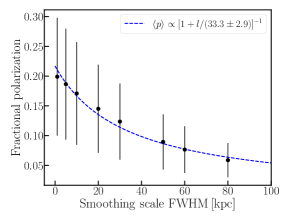
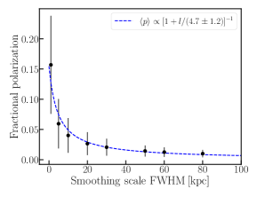
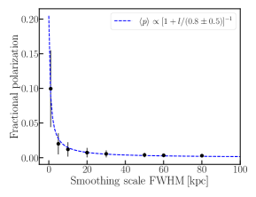
Figure 7: Same as Figure 5 for ${l_{\rm f}}=102.4$ kpc at $t/t_{\rm ed}=20.2$.

5 GHz	1.2 GHz	0.6 GHz

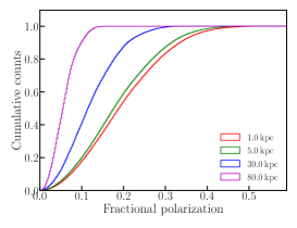
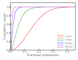
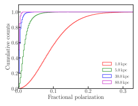
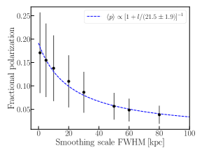
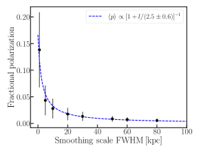
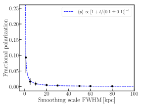
Figure 8: Same as Figure 5 for ${l_{\rm f}}=64$ kpc at $t/t_{\rm ed}=30.6$.

References

References

- Feretti et al. (2012) Feretti, L.; Giovannini, G.; Govoni, F.; Murgia, M. Clusters of galaxies: observational properties of the diffuse radio emission. A&A Rev. 2012, 20, 54, doi:\changeurlcolorblack10.1007/s00159-012-0054-z.
- van Weeren et al. (2019) van Weeren, R.J.; de Gasperin, F.; Akamatsu, H.; Brüggen, M.; Feretti, L.; Kang, H.; Stroe, A.; Zandanel, F. Diffuse Radio Emission from Galaxy Clusters. Space Sci. Rev. 2019, 215, 16, doi:\changeurlcolorblack10.1007/s11214-019-0584-z.
- Vazza et al. (2018) Vazza, F.; Brunetti, G.; Brüggen, M.; Bonafede, A. Resolved magnetic dynamo action in the simulated intracluster medium. MNRAS 2018, 474, 1672–1687, doi:\changeurlcolorblack10.1093/mnras/stx2830.
- Domínguez-Fernández et al. (2019) Domínguez-Fernández, P.; Vazza, F.; Brüggen, M.; Brunetti, G. Dynamical evolution of magnetic fields in the intracluster medium. MNRAS 2019, 486, 623–638, doi:\changeurlcolorblack10.1093/mnras/stz877.
- Sur et al. (2021) Sur, S.; Basu, A.; Subramanian, K. Properties of polarized synchrotron emission from fluctuation-dynamo action—I. Application to galaxy clusters. MNRAS 2021, 501, 3332–3349, doi:\changeurlcolorblack10.1093/mnras/staa3767.
- Clarke et al. (2001) Clarke, T.E.; Kronberg, P.P.; Böhringer, H. A New Radio-X-Ray Probe of Galaxy Cluster Magnetic Fields. ApJ 2001, 547, L111–L114, doi:\changeurlcolorblack10.1086/318896.
- Bonafede et al. (2009) Bonafede, A.; Feretti, L.; Giovannini, G.; Govoni, F.; Murgia, M.; Taylor, G.B.; Ebeling, H.; Allen, S.; Gentile, G.; Pihlström, Y. Revealing the magnetic field in a distant galaxy cluster: discovery of the complex radio emission from MACS J0717.5 +3745. A&A 2009, 503, 707–720, doi:\changeurlcolorblack10.1051/0004-6361/200912520.
- Bonafede et al. (2010) Bonafede, A.; Feretti, L.; Murgia, M.; Govoni, F.; Giovannini, G.; Dallacasa, D.; Dolag, K.; Taylor, G.B. The Coma cluster magnetic field from Faraday rotation measures. A&A 2010, 513, A30, doi:\changeurlcolorblack10.1051/0004-6361/200913696.
- Kierdorf et al. (2017) Kierdorf, M.; Beck, R.; Hoeft, M.; Klein, U.; van Weeren, R.J.; Forman, W.R.; Jones, C. Relics in galaxy clusters at high radio frequencies. A&A 2017, 600, A18, doi:\changeurlcolorblack10.1051/0004-6361/201629570.
- Subramanian et al. (2006) Subramanian, K.; Shukurov, A.; Haugen, N.E.L. Evolving turbulence and magnetic fields in galaxy clusters. MNRAS 2006, 366, 1437–1454, doi:\changeurlcolorblack10.1111/j.1365-2966.2006.09918.x.
- Cho and Ryu (2009) Cho, J.; Ryu, D. Characteristic Lengths of Magnetic Field in Magnetohydrodynamic Turbulence. ApJ 2009, 705, L90–L94, doi:\changeurlcolorblack10.1088/0004-637X/705/1/L90.
- Bhat and Subramanian (2013) Bhat, P.; Subramanian, K. Fluctuation dynamos and their Faraday rotation signatures. MNRAS 2013, 429, 2469–2481, doi:\changeurlcolorblack10.1093/mnras/sts516.
- Porter et al. (2015) Porter, D.H.; Jones, T.W.; Ryu, D. Vorticity, Shocks, and Magnetic Fields in Subsonic, ICM-like Turbulence. ApJ 2015, 810, 93, doi:\changeurlcolorblack10.1088/0004-637X/810/2/93.
- Sur et al. (2018) Sur, S.; Bhat, P.; Subramanian, K. Faraday rotation signatures of fluctuation dynamos in young galaxies. MNRAS 2018, 475, L72–L76, doi:\changeurlcolorblack10.1093/mnrasl/sly007.
- Sur (2019) Sur, S. Decaying turbulence and magnetic fields in galaxy clusters. MNRAS 2019, 488, 3439–3445, doi:\changeurlcolorblack10.1093/mnras/stz1918.
- Brunetti and Jones (2014) Brunetti, G.; Jones, T.W. Cosmic Rays in Galaxy Clusters and Their Nonthermal Emission. Int. J. Mod. Phys. D 2014, 23, 1430007, doi:\changeurlcolorblack10.1142/S0218271814300079.
- Kunz et al. (2011) Kunz, M.W.; Schekochihin, A.A.; Cowley, S.C.; Binney, J.J.; Sanders, J.S. A thermally stable heating mechanism for the intracluster medium: turbulence, magnetic fields and plasma instabilities. MNRAS 2011, 410, 2446–2457, doi:\changeurlcolorblack10.1111/j.1365-2966.2010.17621.x.
- Komarov et al. (2014) Komarov, S.V.; Churazov, E.M.; Schekochihin, A.A.; ZuHone, J.A. Suppression of local heat flux in a turbulent magnetized intracluster medium. MNRAS 2014, 440, 1153–1164, doi:\changeurlcolorblack10.1093/mnras/stu281.
- Roberg-Clark et al. (2016) Roberg-Clark, G.T.; Drake, J.F.; Reynolds, C.S.; Swisdak, M. Suppression of Electron Thermal Conduction in the High Intracluster Medium of Galaxy Clusters. ApJ 2016, 830, L9, doi:\changeurlcolorblack10.3847/2041-8205/830/1/L9.
- Bonafede et al. (2015) Bonafede, A.; Vazza, F.; Brüggen, M.; Akahori, T.; Carretti, E.; Colafrancesco, S.; Feretti, L.; Ferrari, C.; Giovannini, G.; Govoni, F.; et al. Unravelling the origin of large-scale magnetic fields in galaxy clusters and beyond through Faraday Rotation Measures with the SKA. In Proceedings of the Advancing Astrophysics with the Square Kilometre Array (AASKA14), 2015, Trieste, Italy ; p. 95.
- Govoni et al. (2005) Govoni, F.; Murgia, M.; Feretti, L.; Giovannini, G.; Dallacasa, D.; Taylor, G.B. A2255: The first detection of filamentary polarized emission in a radio halo. A&A 2005, 430, L5–L8, doi:\changeurlcolorblack10.1051/0004-6361:200400113.
- Girardi et al. (2016) Girardi, M.; Boschin, W.; Gastaldello, F.; Giovannini, G.; Govoni, F.; Murgia, M.; Barrena, R.; Ettori, S.; Trasatti, M.; Vacca, V. A multiwavelength view of the galaxy cluster Abell 523 and its peculiar diffuse radio source. MNRAS 2016, 456, 2829–2847, doi:\changeurlcolorblack10.1093/mnras/stv2827.
- Pizzo et al. (2011) Pizzo, R.F.; de Bruyn, A.G.; Bernardi, G.; Brentjens, M.A. Deep multi-frequency rotation measure tomography of the galaxy cluster A2255. A&A 2011, 525, A104, doi:\changeurlcolorblack10.1051/0004-6361/201014158.
- Rajpurohit et al. (2021) Rajpurohit, K.; Brunetti, G.; Bonafede, A.; van Weeren, R.J.; Botteon, A.; Vazza, F.; Hoeft, M.; Riseley, C.J.; Bonnassieux, E.; Brienza, M.; et al. Physical insights from the spectrum of the radio halo in MACS J0717.5+3745. A&A 2021, 646, A135, doi:\changeurlcolorblack10.1051/0004-6361/202039591.
- Wittor et al. (2019) Wittor, D.; Hoeft, M.; Vazza, F.; Brüggen, M.; Domínguez-Fernández, P. Polarization of radio relics in galaxy clusters. MNRAS 2019, 490, 3987–4006, doi:\changeurlcolorblack10.1093/mnras/stz2715.
- Böhringer et al. (2016) Böhringer, H.; Chon, G.; Kronberg, P.P. The Cosmic Large-Scale Structure in X-rays (CLASSIX) Cluster Survey. I. Probing galaxy cluster magnetic fields with line of sight rotation measures. A&A 2016, 596, A22, doi:\changeurlcolorblack10.1051/0004-6361/201628873.
- Vacca et al. (2010) Vacca, V.; Murgia, M.; Govoni, F.; Feretti, L.; Giovannini, G.; Orrù, E.; Bonafede, A. The intracluster magnetic field power spectrum in Abell 665. A&A 2010, 514, A71, doi:\changeurlcolorblack10.1051/0004-6361/200913060.
- Schekochihin et al. (2004) Schekochihin, A.A.; Cowley, S.C.; Taylor, S.F.; Maron, J.L.; McWilliams, J.C. Simulations of the Small-Scale Turbulent Dynamo. ApJ 2004, 612, 276–307, doi:\changeurlcolorblack10.1086/422547.
- Brandenburg and Subramanian (2005) Brandenburg, A.; Subramanian, K. Astrophysical magnetic fields and nonlinear dynamo theory. Phys. Rep. 2005, 417, 1–209, doi:\changeurlcolorblack10.1016/j.physrep.2005.06.005.
- Seta et al. (2020) Seta, A.; Bushby, P.J.; Shukurov, A.; Wood, T.S. Saturation mechanism of the fluctuation dynamo at PrM 1. Phys. Rev. Fluids 2020, 5, 043702, doi:\changeurlcolorblack10.1103/PhysRevFluids.5.043702.
- Basu et al. (2019) Basu, A.; Fletcher, A.; Mao, S.A.; Burkhart, B.; Beck, R.; Schnitzeler, D. An In-depth Investigation of Faraday Depth Spectrum Using Synthetic Observations of Turbulent MHD Simulations. Galaxies 2019, 7, 89, doi:\changeurlcolorblack10.3390/galaxies7040089.
- Fryxell et al. (2000) Fryxell, B.; Olson, K.; Ricker, P.; Timmes, F.X.; Zingale, M.; Lamb, D.Q.; MacNeice, P.; Rosner, R.; Truran, J.W.; Tufo, H. FLASH: An Adaptive Mesh Hydrodynamics Code for Modeling Astrophysical Thermonuclear Flashes. ApJS 2000, 131, 273–334. doi:\changeurlcolorblack10.1086/317361.
- Miniati (2015) Miniati, F. The Matryoshka Run. II. Time-dependent Turbulence Statistics, Stochastic Particle Acceleration, and Microphysics Impact in a Massive Galaxy Cluster. ApJ 2015, 800, 60, doi:\changeurlcolorblack10.1088/0004-637X/800/1/60.
- Vazza et al. (2017) Vazza, F.; Jones, T.W.; Brüggen, M.; Brunetti, G.; Gheller, C.; Porter, D.; Ryu, D. Turbulence and vorticity in Galaxy clusters generated by structure formation. MNRAS 2017, 464, 210–230, doi:\changeurlcolorblack10.1093/mnras/stw2351.
- Wittor et al. (2017) Wittor, D.; Jones, T.; Vazza, F.; Brüggen, M. Evolution of vorticity and enstrophy in the intracluster medium. MNRAS 2017, 471, 3212–3225, doi:\changeurlcolorblack10.1093/mnras/stx1769.
- Vallés-Pérez et al. (2021) Vallés-Pérez, D.; Planelles, S.; Quilis, V. Troubled cosmic flows: turbulence, enstrophy, and helicity from the assembly history of the intracluster medium. MNRAS 2021, 504, 510–527, doi:\changeurlcolorblack10.1093/mnras/stab880.
- Hitomi Collaboration: Aharonian et al. (2018) Aharonian, F.; Akamatsu, H.; Akimoto, F.; Allen, S.W.; Angelini, L.; Audard, M.; Awaki, H.; Axelsson, M.; Bamba, A.; Bautz, M.W.; et al. Atmospheric gas dynamics in the Perseus cluster observed with Hitomi. PASJ 2018, 70, 9, doi:\changeurlcolorblack10.1093/pasj/psx138.
- Churazov et al. (2012) Churazov, E.; Vikhlinin, A.; Zhuravleva, I.; Schekochihin, A.; Parrish, I.; Sunyaev, R.; Forman, W.; Böhringer, H.; Randall, S. X-ray surface brightness and gas density fluctuations in the Coma cluster. MNRAS 2012, 421, 1123–1135, doi:\changeurlcolorblack10.1111/j.1365-2966.2011.20372.x.
- Zhuravleva et al. (2019) Zhuravleva, I.; Churazov, E.; Schekochihin, A.A.; Allen, S.W.; Vikhlinin, A.; Werner, N. Suppressed effective viscosity in the bulk intergalactic plasma. Nat. Astron. 2019, 3, 832–837, doi:\changeurlcolorblack10.1038/s41550-019-0794-z.
- Sarazin (1988) Sarazin, C.L. X-ray Emission from Clusters of Galaxies; Cambridge University Press: Cambridge, UK, 1988.
- Brentjens and de Bruyn (2005) Brentjens, M.A.; de Bruyn, A.G. Faraday rotation measure synthesis. A&A 2005, 441, 1217–1228, doi:\changeurlcolorblack10.1051/0004-6361:20052990.
- Heald et al. (2009) Heald, G.; Braun, R.; Edmonds, R. The Westerbork SINGS survey. II Polarization, Faraday rotation, and magnetic fields. A&A 2009, 503, 409–435, doi:\changeurlcolorblack10.1051/0004-6361/200912240.
- Cuciti et al. (2021) Cuciti, V.; Cassano, R.; Brunetti, G.; Dallacasa, D.; van Weeren, R.J.; Giacintucci, S.; Bonafede, A.; de Gasperin, F.; Ettori, S.; Kale, R.; et al. Radio halos in a mass-selected sample of 75 galaxy clusters. I. Sample selection and data analysis. A&A 2021, 647, A50, doi:\changeurlcolorblack10.1051/0004-6361/202039206.
- Govoni and Feretti (2004) Govoni, F.; Feretti, L. Magnetic Fields in Clusters of Galaxies. Int. J. Mod. Phys. D 2004, 13, 1549–1594, doi:\changeurlcolorblack10.1142/S0218271804005080.
- Thierbach et al. (2003) Thierbach, M.; Klein, U.; Wielebinski, R. The diffuse radio emission from the Coma cluster at 2.675 GHz and 4.85 GHz. A&A 2003, 397, 53–61, doi:\changeurlcolorblack10.1051/0004-6361:20021474.
- Sokoloff et al. (1998) Sokoloff, D.; Bykov, A.; Shukurov, A.; Berkhuijsen, E.; Beck, R.; Poezd, A. Depolarization and Faraday effects in galaxies. MNRAS 1998, 299, 189–206, doi:\changeurlcolorblack10.1046/j.1365-8711.1998.01782.x.
- O’Sullivan et al. (2012) O’Sullivan, S.; Brown, S.; Robishaw, T.; Schnitzeler, D.; McClure-Griffiths, N.; Feain, I.; Taylor, A.; Gaensler, B.; Landecker, T.; Harvey-Smith, L.; et al. Complex Faraday depth structure of active galactic nuclei as revealed by broad-band radio polarimetry. MNRAS 2012, 421, 3300–3315, doi:\changeurlcolorblack10.1111/j.1365-2966.2012.20554.x.
- O’Sullivan et al. (2015) O’Sullivan, S.P.; Gaensler, B.M.; Lara-López, M.A.; van Velzen, S.; Banfield, J.K.; Farnes, J.S. The Magnetic Field and Polarization Properties of Radio Galaxies in Different Accretion States. ApJ 2015, 806, 83, doi:\changeurlcolorblack10.1088/0004-637X/806/1/83.
- Akahori et al. (2016) Akahori, T.; Ryu, D.; Gaensler, B.M. Fast Radio Bursts as Probes of Magnetic Fields in the Intergalactic Medium. ApJ 2016, 824, 105, doi:\changeurlcolorblack10.3847/0004-637X/824/2/105.
- Vazza et al. (2014) Vazza, F.; Brüggen, M.; Gheller, C.; Wang, P. On the amplification of magnetic fields in cosmic filaments and galaxy clusters. MNRAS 2014, 445, 3706–3722, doi:\changeurlcolorblack10.1093/mnras/stu1896.
- O’Sullivan et al. (2019) O’Sullivan, S.P.; Machalski, J.; Van Eck, C.L.; Heald, G.; Brüggen, M.; Fynbo, J.P.U.; Heintz, K.E.; Lara-Lopez, M.A.; Vacca, V.; Hardcastle, M.J.; et al. The intergalactic magnetic field probed by a giant radio galaxy. A&A 2019, 622, A16, doi:\changeurlcolorblack10.1051/0004-6361/201833832.
- Briel et al. (1992) Briel, U.G.; Henry, J.P.; Boehringer, H. Observation of the Coma cluster of galaxies with ROSAT during the all-sky-survey. A&A 1992, 259, L31–L34.
- Norman and Bryan (1999) Norman, M.L.; Bryan, G.L., Cluster Turbulence. In The Radio Galaxy Messier 87; Röser, H.J., Meisenheimer, K., Eds.; Springer: Berlin/Heidelberg; 1999; Volume 530, p. 106, doi:\changeurlcolorblack10.1007/BFb0106425.
- Ryu et al. (2008) Ryu, D.; Kang, H.; Cho, J.; Das, S. Turbulence and Magnetic Fields in the Large-Scale Structure of the Universe. Science 2008, 320, 909, doi:\changeurlcolorblack10.1126/science.1154923.
- Xu et al. (2012) Xu, H.; Govoni, F.; Murgia, M.; Li, H.; Collins, D.C.; Norman, M.L.; Cen, R.; Feretti, L.; Giovannini, G. Comparisons of Cosmological Magnetohydrodynamic Galaxy Cluster Simulations to Radio Observations. ApJ 2012, 759, 40, doi:\changeurlcolorblack10.1088/0004-637X/759/1/40.
- Donnert et al. (2009) Donnert, J.; Dolag, K.; Lesch, H.; Müller, E. Cluster magnetic fields from galactic outflows. MNRAS 2009, 392, 1008–1021, doi:\changeurlcolorblack10.1111/j.1365-2966.2008.14132.x.
- Dubois et al. (2012) Dubois, Y.; Devriendt, J.; Slyz, A.; Teyssier, R. Self-regulated growth of supermassive black holes by a dual jet–heating active galactic nucleus feedback mechanism: methods, tests and implications for cosmological simulations. MNRAS 2012, 420, 2662–2683, doi:\changeurlcolorblack10.1111/j.1365-2966.2011.20236.x.
- Pakmor et al. (2016) Pakmor, R.; Pfrommer, C.; Simpson, C.M.; Springel, V. Galactic Winds Driven by Isotropic and Anisotropic Cosmic-Ray Diffusion in Disk Galaxies. ApJ 2016, 824, L30, doi:\changeurlcolorblack10.3847/2041-8205/824/2/L30.
- Wiener et al. (2017) Wiener, J.; Pfrommer, C.; Peng Oh, S. Cosmic ray-driven galactic winds: streaming or diffusion? MNRAS 2017, 467, 906–921, doi:\changeurlcolorblack10.1093/mnras/stx127.
- Fabian (2012) Fabian, A.C. Observational Evidence of Active Galactic Nuclei Feedback. ARA&A 2012, 50, 455–489, doi:\changeurlcolorblack10.1146/annurev-astro-081811-125521.
- Bourne and Sijacki (2017) Bourne, M.A.; Sijacki, D. AGN jet feedback on a moving mesh: cocoon inflation, gas flows and turbulence. MNRAS 2017, 472, 4707–4735, doi:\changeurlcolorblack10.1093/mnras/stx2269.
- Ehlert et al. (2021) Ehlert, K.; Weinberger, R.; Pfrommer, C.; Springel, V. Connecting turbulent velocities and magnetic fields in galaxy cluster simulations with active galactic nuclei jets. MNRAS 2021, 503, 1327–1344, doi:\changeurlcolorblack10.1093/mnras/stab551.
- Braun et al. (2019) Braun, R.; Bonaldi, A.; Bourke, T.; Keane, E.; Wagg, J. Anticipated Performance of the Square Kilometre Array—Phase 1 (SKA1). arXiv 2019, arXiv:1912.12699.
- Yuan et al. (2015) Yuan, Z.S.; Han, J.L.; Wen, Z.L. The Scaling Relations and the Fundamental Plane for Radio Halos and Relics of Galaxy Clusters. ApJ 2015, 813, 77, doi:\changeurlcolorblack10.1088/0004-637X/813/1/77.
- Astropy Collaboration et al. (2013) Astropy Collaboration; Robitaille, T.P.; Tollerud, E.J.; Greenfield, P.; Droettboom, M.; Bray, E.; Aldcroft, T.; Davis, M.; Ginsburg, A.; Price-Whelan, A.M.; et al. Astropy: A community Python package for astronomy. A&A 2013, 558, A33, doi:\changeurlcolorblack10.1051/0004-6361/201322068.
- Price-Whelan et al. (2018) Price-Whelan, A.M.; Sipőcz, B.M.; Günther, H.M.; Lim, P.L.; Crawford, S.M.; Conseil, S.; Shupe, D.L.; Craig, M.W.; Dencheva, N.; Ginsburg, A.; et al. The Astropy Project: Building an Open-science Project and Status of the v2.0 Core Package. AJ 2018, 156, 123. doi:\changeurlcolorblack10.3847/1538-3881/aabc4f.
- van der Walt et al. (2011) van der Walt, S.; Colbert, S.C.; Varoquaux, G. The NumPy Array: A Structure for Efficient Numerical Computation. Comput. Sci. Eng. 2011, 13, 22–30.
- Hunter (2007) Hunter, J.D. Matplotlib: A 2D graphics environment. Comput. Sci. Eng. 2007, 9, 90–95, doi:\changeurlcolorblack10.1109/MCSE.2007.55.