Look Who’s Talking: Interpretable Machine Learning for Assessing Italian SMEs Credit Default

Abstract

Academic research and the financial industry have recently paid great attention to Machine Learning algorithms due to their power to solve complex learning tasks. In the field of firms’ default prediction, however, the lack of interpretability has prevented the extensive adoption of the black-box type of models. To overcome this drawback and maintain the high performances of black-boxes, this paper relies on a model-agnostic approach. Accumulated Local Effects and Shapley values are used to shape the predictors’ impact on the likelihood of default and rank them according to their contribution to the model outcome. Prediction is achieved by two Machine Learning algorithms (eXtreme Gradient Boosting and FeedForward Neural Network) compared with three standard discriminant models. Results show that our analysis of the Italian Small and Medium Enterprises manufacturing industry benefits from the overall highest classification power by the eXtreme Gradient Boosting algorithm without giving up a rich interpretation framework.

Keywords: Risk Analysis, Machine Learning, Intepretability, Small and Medium Sized Enterprises, Default Prediction.

1 Introduction

The economy of the European Union (EU) is deeply grounded into Small and Medium Enterprises (SMEs). SMEs represent about 99.8% of the active enterprises in the EU-28 non-financial business sector (NFBS), accounting for almost 60% of value-added within the NFBS and fostering the workforce of the EU with two out of every three jobs (European Commission, 2019a).

Thus, there is a wide literature covering various economic aspects of SMEs, with a particular attention to default prediction (for an up-to-date review see Ciampi et al., 2021), which is of interest not only for scholars but also for practitioners such as financial intermediaries and for policy makers in their effort to support SMEs and to ease credit constraints to which they are naturally exposed (Andries et al., 2018; Cornille et al., 2019).

Whether it is for private credit-risk assessment or for public funding, independently on the type of data imputed to measure the health status of a firm, prediction of default should success in two aspects: maximise correct classification and clarify the role of the variables involved in the process. Most of the times, the contributions based on Machine Learning (ML) techniques neglect the latter aspect, being rather focused on the former, often with better results with respect to parametric techniques that provide, on the contrary, a clear framework for interpretation. In other words ML techniques rarely deal with interpretability which, according to a recent document released by the European Commission, should be kept "in mind from the start" (European Commission, 2019b).

Interpretability is central when a model is to be applied in the practice, both in terms of managerial choices and compliance: it is a fundamental requisite to bring a model into production. Interpretable models allow risk managers and decision-makers to understand its validity by looking at its inner workings and helping in the calibration process. The European Commission itself encourages organizations to build trustworthy Artificial Intelligence (AI) systems (including ML techniques) around several pillars: one of them is transparency, which encompasses traceability, explainability and open communication about the limitations of the AI system (High-Level Expert Group on Artificial Intelligence, European Commission, 2020).

Consequently, ML models -no matter how good in classifying default- should be made readable or their inherent uninterpretable nature will prevent their spreading in the literature on firms’ default prediction as well as their use in contexts regulated by transparency norms.

This work try to fill this gap by applying two different kind of ML models (FeedForward Neural Network (Haykin, 1999) and eXtreme Gradient Boosting (Chen and Guestrin, 2016) to Italian Manufacturing SMEs’ default prediction, with a special attention to interpretability. Italy represents an ideal testing ground for SMEs default prediction since its economic framework is even more shaped by firms up to this size with respect to the average EU country (European Commission, 2019a). Default was assessed on the basis of the firms’ accounting information retrieved from Orbis, a Bureau van Dijk (BvD) dataset.

The main original contribution of the paper is to address ML models’ interpretability into the context of default prediction. Our approach is based on model agnostic-techniques and adds Accumulated Local Effects (ALEs, Apley and Zhu, 2020) to the Shapley values (already applied in Bussmann et al., 2021). Using these techniques we can rank the variables in terms of their contribution to the classification and determine their impact on default prediction, characterizing risky thresholds and non-linear patterns. Robustness of the ML models hyperparameters was taken care of by Montecarlo Cross-Validation and substantial class imbalance between defaulted and survived firms was reduced through undersampling of the latter into the cross-validation training sets. Another contribution of the paper is the benchmarking of the ML models’ outcome with Logistic, Probit and with Binary Generalized Extreme Value Additive (BGEVA) classifications, both according to standard performances metrics and to the role played by the different variables. We also supply ALEs for the parametric models, in order to get additional insights with respect to variables significance and to guarantee a common ground for comparison.

We obtain at least three interesting results. First, thanks to our research design, all the proposed models work fairly well according to all the metrics. Second, eXtreme Gradient Boosting (XGBoost) outperformed the others mainly for total classification accuracy and default prediction rate. Third, the impact of the variables retrieved from XGBoost is fully consistent with the economic literature, whereas the same cannot be said for the competing models.

The remainder of the paper is organized as follows. Section 2 gives an overview of the (necessarily) recent literature concerning ML intepretability. Section 3 provides a description of the dataset and of the features we use throughout the modelling. Section 4 discusses our methodology, briefly reviewing the models fundamentals, the techniques employed for interpretability and the research design. Section 5 presents the results and discusses the most relevant findings. Section 6 concludes.

2 Literature review

The ability to predict corporate failure has been largely investigated in credit risk literature since the 1970s (Laitinen and Gin Chong, 1999). On the one hand, the academic interest in the topic has grown after the global financial crisis (2007-2009) that has highlighted the need for more consistent models to assess the risk of failure of SMEs (Oliveira et al., 2017) and it is renewed today with the current pandemic impact on the companies of all sizes (Ciampi et al., 2021). On the other hand, a good part of the financial industry has shown great attention to statistical algorithms that prioritize the pursuit of predictive power. Such a trend has been registered by recent surveys, showing that credit institutions are gradually embracing ML techniques in different areas of credit risk management, credit scoring and monitoring (Bank of England, 2019; Alonso and Carbó, 2020; Institute of International Finance, 2020). Among all, the biggest annual growth in the adoption of highly performing algorithms has been observed in the SMEs sector (Institute of International Finance, 2019).

For these reasons, new modeling techniques have been successfully employed in predicting SMEs default, including Deep Learning (Mai et al., 2019), boosting (Moscatelli et al., 2020; Kou et al., 2021), Support Vector Machine (Kim and Sohn, 2010; Gordini, 2014; Zhang et al., 2015), Neural Networks (Alfaro et al., 2008; Ciampi and Gordini, 2013; Geng et al., 2015) and two-stage classification (du Jardin, 2016), to name a few. However, they have been applied mainly in order to improve classification accuracy with respect to the standard linear models, rather than in terms of causality patterns. But the latter is no longer a negligible aspect, both for academic research and for management of regulated financial services: it has become overriding, since the European Commission and other European Institutions released a number of regulatory standards on Machine Learning modeling.

The Ethics Guidelines for Trustworthy AI (European Commission, 2019b) and the Report on Big Data and Advanced Analytics (European Banking Authority, 2020) illustrate the principle of explicability of ML algorithms that have to be transparent and fully interpretable, including for those directly and indirectly affected. Indeed, as the Commission points out, predictions, even accurate, without explainability measures are not able to foster responsible and sustainable AI innovation. The pillar of transparency (fourth among seven), somewhat combines explainability and interpretability of a model, referring to interpretability as the "concept of comprehensibility, explainability, or understandability" (High-Level Expert Group on Artificial Intelligence, European Commission, 2020).

The difference in meaning between interpretability and explainability, synonymous in the dictionary, has been addressed by the recent ML literature which recognizes the two words a conceptual distinction related to different properties of the model and knowledge aspects (Doran et al., 2017; Lipton, 2018). A clear indication about the distinction is given by Montavon et al. (2018) that defines interpretation as a mapping of an abstract concept into a domain that the human expert can perceive and comprehend and explanation as a collection of features of the interpretable domain that have contributed to a given example to produce a decision. Roughly speaking, interpretability is defined as the ability to spell out or to provide the meaning in understandable terms to a human (Doshi-Velez and Kim, 2017; Guidotti et al., 2018), whereas explainability is identified as the capacity of revealing the causes underlying the decision driven by a ML method (Arrieta et al., 2020).

There are several approaches to ML interpretability in the literature, classified in two main categories: ante-hoc and post-hoc methods. Ante-hoc methods employ intrinsically interpretable models (e.g., simple decision tree or regression models, also called white-box) characterized by a simple structure. They rely on model-specific interpretations depending on examination of internal model parameters. Post-hoc methods instead provide a reconstructed interpretation of decision records produced by a black-box model in a reverse engineering logic (Ribeiro et al., 2016a; Du et al., 2019). These methods reckon on model-agnostic interpretation where internal model parameters are not inspected.

So far, ante-hoc approaches were widely used in the SMEs default prediction literature that counts contributions employing mainly white-box models as Logistic regression (see for example Sohn and Kim, 2007; Lin et al., 2012; Modina and Pietrovito, 2014; Ciampi, 2015), Survival analysis (Holmes et al., 2010; Gupta et al., 2015; El Kalak and Hudson, 2016; Gupta et al., 2018) or Generalised Extreme Value regression (Calabrese et al., 2016). The empirical evidences and the variables’ effect on the outcome are interpreted in an inferential testing setting, so that the impact of the predictors and the results’ implications are always clear to the reader. An alternative strategy can be found in Liberati et al. (2017) that interprets a kernel-based classifier for default prediction via a surrogate model, but the results and the variables impact are conditioned to the regression fit to the data.

On the contrary, post-hoc methods have been rarely used in this field and comprehend Partial Dependence (PD) plots (Friedman, 2001), Local Interpretable Model-agnostic Explanations (LIME) (Ribeiro et al., 2016b) and the SHAP values (Lundberg and Lee, 2017), all of them providing detailed model-agnostic interpretation of the complex ML algorithms employed. Jones and Wang (2019), Sigrist and Hirnschall (2019) and Jabeur et al. (2021) used the PD to identify the relevant variables’ subset and to measure the change of the average probability of default with respect to the single features. Stevenson et al. (2021) and Yıldırım et al. (2021), instead, applied LIME and SHAP values to rank the most important variables and to provide the features impacts on the output prediction respectively. In this paper we employ the Accumulated Local Effects (ALE), a model-agnostic technique that represents a suitable alternative to PDs when the features are highly correlated, without providing incoherent values (Apley and Zhu, 2020). Since ALE is a newest approach, its usage is far more limited and it has not yet spread in the bankruptcy prediction area. An isolate application to the recovery rate forecasting of non-performing loans can be encountered in the credit risk field (Bellotti et al., 2021).

3 Data Description

The data of this study are retrieved from BvD database, which provides financial and accounting ratios from balance sheets of the European private companies. We have restricted our focus on Italian manufacturing SMEs for several reasons. Italy is the second-largest manufacturing country in the EU (Bellandi et al., 2020) and this sector generates more than 30% of the Italian GDP (Eurostat, 2018). Differently from SMEs in other EU countries, Italian SMEs trade substantially more than large firms and manufacturing, in particular, drives both import and exports (Abel-Koch et al., 2018). Moreover, according to Ciampi et al. (2009) and Ciampi and Gordini (2013), predictive models have better performances when trained for a specific sector as this avoids pooling heterogeneous firms.

To define our sample, we filtered the database both by country and NACE codes (from 10 to 33) and we employed the European Commission definition (EU, 2003) of Small and Medium Enterprises. We retrieved only firms with annual turnover of fewer than 50 million euros, the number of employees lower than 250 and a balance sheet of fewer than 43 million euros. Among those, we classified as defaults all the enterprises that entered bankruptcy or a liquidation procedure, as well as active companies that had not repaid debt (default of payment), active companies in administration or receivership or under a scheme of the arrangement, (insolvency proceedings), which in Orbis are also considered in default. Consistently with the literature, we excluded dissolved firms that no longer exist as a legal entity when the reason for dissolution is not specified (Altman and Sabato, 2007; Altman et al., 2010; Andreeva et al., 2016). This category in fact encompasses firms that may not necessarily experience financial difficulties. The resulting dataset contains 105,058 SMEs with a proportion of 1.72% (1,807) failed companies.

The accounting indicators, which refer to 2016 for predicting the status of the firms in 2017, have been selected among the most frequently used in the SMEs default literature and are the following:

• Cash flow: computed as net income plus depreciations (Lin et al., 2012; Calabrese and Osmetti, 2013; Ciampi and Gordini, 2013; Succurro et al., 2014; Michala et al., 2013; Jones et al., 2015; Andreeva et al., 2016);

• Gearing ratio: computed as the ratio between total debt and total assets (Altman and Sabato, 2007; Ciampi et al., 2009; Fantazzini and Figini, 2009; Altman et al., 2010; Lin et al., 2012; Jones et al., 2015; Andreeva et al., 2016; Psillaki et al., 2010);

• Number of employees, as a size measure from an input perspective (Andreeva et al., 2016);

• Profit margin: measured as profit/loss before tax over the operating revenue (Ciampi et al., 2009; Altman et al., 2010; Lin et al., 2012; Ciampi and Gordini, 2013; Andreeva et al., 2016);

• ROCE: computed as profit/loss before tax over capital employed, which is given as total assets minus current liabilities (Lin et al., 2012; Andreeva et al., 2016; Nehrebecka, 2018);

• ROE: computed as profit/loss before tax over shareholders’ funds (Ciampi et al., 2009; Altman et al., 2010; Ciampi and Gordini, 2013; Succurro et al., 2014; Jones et al., 2015; Andreeva et al., 2016);

• Sales: in thousands Euro, measuring the output side of firm size (Succurro et al., 2014);

• Solvency ratio: computed as shareholders’ funds over total assets (Ciampi et al., 2009; Calabrese and Osmetti, 2013; Jones et al., 2015; Andreeva et al., 2016; Calabrese et al., 2016; Nehrebecka, 2018);

• Total assets: in thousands Euro, as a measure of total firm resources (Lin et al., 2012; Michala et al., 2013; Andreeva et al., 2016).

As a quick preview of the expected relationship between the single predictors and the likelihood of default, we have computed the average values and standard deviations of the variables separately for survived and defaulted firms (see table 1).

Table 1: Summary statistics by survived and failed firms

	Survived		Failed
Variable	Mean	St. dev.	Mean	St. dev.
Cash flow	236,802	934,877	-278,521	1.636,028
Gearing ratio	24,807	23,093	22,166	26,01
Number of employees	16,506	24,385	11,08	19,531
Profit margin	-2,736	610,488	-106,845	2.190,012
ROCE	12,335	516,765	66,367	2.284,001
ROE	23,02	314,135	7,146	971,112
Sales	3.427,163	6.301,229	1.259,695	2.940,01
Solvency ratio	27,101	24,315	-1,044	37,342
Total assets	3.904,129	12.098,09	1.921,689	5.149,559

In line with Andreeva et al. (2016), we can see on average weakest liquidity, smallest size and deficient leverage for defaulted firms. The Profit margin and ROE are highest for surviving firms, whereas the remaining profitability index, ROCE, shows a larger mean among defaulted firms. ROCE should be, according to common sense, negatively related to default. However, some studies found its impact non-significant coherently with the low-equity dependency of small businesses (Ahelegbey et al., 2019; Giudici et al., 2020), while others attest a positive effect of ROCE on default with a caveat for large values (Calabrese et al., 2016).

4 Methodology

4.1 White-box versus black-box models

The models we apply can be broadly classified as white-box, or interpretable, and black-box but post-hoc interpretable in the model-agnostic framework.

In the first category, Logistic Regression (LR) and Probit were selected among the most recurrent models in the economics literature, where the accent on the factors impacting default is certainly of primary importance. These models frequently serve as a benchmark for classification when a new method is proposed. The third model, BGEVA (Calabrese and Osmetti, 2013), comes from the Operational Research literature and is based on the quantile function of a Generalized Extreme Value random variable. The main strengths of BGEVA are robustness, accounting for non-linearities and preserving interpretability.

The black-box models we use are XGBoost and FeedForward Neural Network (FANN). These models are by nature uninterpretable since the explanatory variables pass multiple trees (XGBoost) or layers (FANN), thus generating an output for which an understandable explanation cannot be provided.

The XGBoost algorithm was found to provide the best performance in default prediction with respect to LR, Linear Discriminant Analysis, and Artificial Neural Networks (Petropoulos et al., 2019; Bussmann et al., 2021). The algorithm builds a sequence of shallow decision trees, which are trees with few leaves. Considering a single tree one would get an interpretable model taking the following functional form:

$$f(x)=\sum^{M}_{m=1}\theta_{m}I(x\in R_{m})$$ (1)

where $M$ covers the whole input space with $R_{1},...R_{M}$ non-overlapping partitions, $I(\cdot)$ is the indicator function, and $\theta_{m}$ is the coefficient associated with partition $R_{m}$. In this layout, each subsequent tree learns from the previous one and improves the prediction (Friedman, 2001).

As a competing black-box model we chose the FANN, which is widely used and well performing in SMEs’ default prediction (Ciampi et al., 2021) and in several works on retail credit risk modeling (West, 2000; Baesens et al., 2003; West et al., 2005). FANN consists of a direct acyclic network of nodes organized in densely connected layers, where inputs, after been weighted and shifted by a bias term, are fed into the node’s activation function and influence each subsequent layer until the final output layer. In a simple classification task, in which only one hidden layer is necessary, a FANN can be described by:

$$P(y=1|x)=\sum^{M}_{m=1}w^{1}_{m}a(w^{0}_{m}x+b_{m})$$ (2)

where the weighted combination of the inputs is shifted by the bias $b$ and activated by the function $a$. Note that imposing $a(\cdot)$ as the sigmoid function in equation 2 the model collapses to a LR.

4.2 Model-agnostic interpretability

To achieve the goal of interpretability we make use of two different and complementary model-agnostic techniques. First, we use the global Shapley Values (Shapley, 1953) to provide comparable information on the single feature contributions to the model output. Global Shapley Values have been already proposed in the SMEs default prediction literature by Bussmann et al. (2021).

However, global Shapley Values do not provide any information about the direction and shape of the variable effects. To get this information, we resort to ALEs (Apley and Zhu, 2020). ALEs, contrary to Shapley Values, offer a visualization of the path according to which the single variables impact on the estimated probability of default.

To further clarify the improvement that ALEs bring to interpretability in our setting, we briefly contextualize the method and sketch its fundamentals.

The first model-agnostic approach for ML models’ interpretation to appear in the literature was Partial Dependence (PD), proposed by Friedman (1991) in the early ’90s. PD plots evaluate the change in the average predicted value as specified features vary over their marginal distribution (Goldstein et al., 2015). In other words, they measure the dependence of the outcome on a single feature when all of the others are marginalized out. Since their first formulation, PD plots have been used extensively in many fields but seldom in the credit risk literature, whit a recent application by Su et al. (2021).

One of the main criticisms moved to PD is on its managing the relationships within features. The evaluation of PD on all the possible feature configurations carries the risk of computing points outside the data envelope: such points, intrinsically artificial, can result in a misleading effect of some features when working on real datasets.

Due to this fallacy, and because of the renewed interest in complex deep learning models as Artificial Neural Networks, many new methodologies have been proposed. With Average Marginal Effects (AMEs), Hechtlinger (2016) suggested to condition the PD to specified values of the data envelope. Ribeiro et al. (2016b) went the opposite direction presenting a local approximation of the model through simpler linear models, the so-called Local Interpretable Model-agnostic Explanations (LIME). In subsequent research, they also worked on rule-based local explanations of complex black-box models (Ribeiro et al., 2018). Shapley Additive exPlanations (SHAP) was introduced by Lundberg and Lee (2017) to provide a human understandable and local Shapley evaluation.

In this framework, ALEs constitute a further refinement of both PD and AMEs. They avoid the PD plots-drawback of assessing variables’ effects outside the data envelope, generally occurring when features are highly correlated (Apley and Zhu, 2020), as in the case of many accounting indicators (Ciampi et al., 2009; Altman et al., 2010; Ciampi, 2015). Furthermore, ALEs do not simply condition on specified values of the data envelope as AMEs do, but take first-order differences conditional on the feature space partitioning, eventually eliminating possible bias derived from features’ relationships.

Specifically, computing the ALE implies the evaluation of the following type of function:

$$ALE_{\hat{f},S}(x)=\int_{z_{0,S}}^{x}\left[\int\frac{\delta\hat{f}(z_{S},X_{\setminus S})}{\delta z_{S}}d\mathcal{P}(X_{\setminus S}|z_{S})\right]dz_{S}-constant$$ (3)

where:

• $\hat{f}$ is the black-box model;

• $S$ is the subset of variables’ index;

• $X$ is the matrix containing all the variables;

• $x$ is the vector containing the feature values per observation;

• $z$ identifies the boundaries of the K partitions, such that $z_{0,S}=min(x_{S})$.

The expression in equation 3 is in principle not model-agnostic as it requires accessing the gradient of the model: $\nabla_{z_{S}}\hat{f}=\frac{\delta\hat{f}(z_{S},X_{\setminus S})}{\delta z_{S}}$ but this is not known or even not existent in certain black-boxes. As a replacement, finite differences are taken to the boundaries of the partitions, $z_{k-1}$ and $z_{k}$.

Hence, the resulting formula to evaluate ALEs is:

$$ALE_{\hat{f},S}(x_{S})=\sum_{k=1}^{k_{S}(x)}\frac{1}{n_{S}(k)}\sum_{i:x_{S}^{(i)}\in N_{S}(k)}\left[\hat{f}(z_{k,j},x_{\setminus S}^{(i)})-\hat{f}(z_{k-1,j},x_{\setminus S}^{(i)})\right]-\frac{1}{n}\sum_{i=1}^{n}ALE_{\hat{f},S}(x_{S}^{(i)})$$ (4)

The replacement of the constant term in equation 3 by $-\frac{1}{n}\sum_{i=1}^{n}ALE_{\hat{f},S}(x_{S}^{(i)})$ in equation 4 centers the plot, which is something missing in PD. This makes it clear that, by evaluating predictions’ finite differences conditional on $S$ and integrating the derivative over features $S$, ALEs disentangles the interaction between covariates. This way the main disadvantage of PD is solved.

4.3 Research design

Our research design has been carried out according to Lessmann et al. (2015). We split the initial dataset into training (70%) and test (30%) sets (James et al., 2013). Then, through the Monte Carlo Cross-Validation procedure (Xu and Liang, 2001), we estimate the models parameters and validate the estimated rules. More in detail, at each iteration we create a sub-training set and a validation set via random sampling without replacement so that the models learn from the training set whereas the assessment, based on performance metrics, is done on the validation set. This way, we also tune the hyperparameters of the algorithms when necessary.

The training set serves as well to compute the Shapley values, based on the optimal rule, and to calculate the ALEs with corresponding bootstrap non-parametric confidence intervals (Davison and Kuonen, 2002; Apley and Zhu, 2020). Finally, we evaluated the models’ performance on the hold-out sample (test set).

We took into account also the severe unbalance in favour of survived firms to avoid over-classification of the majority class (Baesens et al., 2021). In the learning phase, we employed perfectly balanced samples, obtained through random under-sampling of the survived firms. This sampling scheme combined the best classification performances with a drastic reduction in the computation time. Obviously the undersampling scheme was applied only to the training data, to avoid over-optimistic performance metrics on either the validation or the test set (Gong and Kim, 2017; Santos et al., 2018).

5 Results

The results are organized according to the performance and interpretation of the five models.

The performance is measured by the proportion of failed and survived firms correctly identified (sensitivity and specificity) as well as by two global perfomance metrics: the Area Under the Receiver Operating Curve (AUC) and the H-measure (see Table 2). The need for an additional indicator of global performance other than the AUC is motivated to assure robustness of the results. The AUC has indeed several advantages in providing consistent classifier performance (Lin et al., 2012) and is widely adopted by practitioners (Lessmann et al., 2015), but it suffers from using different misclassification cost distributions for different classifiers as outlined by Hand (2009) and Hand and Anagnostopoulos (2013). Thus, we add the H-measure that normalizes classifiers’ cost distribution based on the expected minimum misclassification loss.

Second, we cross-compare the role and weight of the variables among models and contextualize the results within the literature. The post-hoc interpretation of the black-box models is based on the Shapley values and ALEs. We report the ALEs also for interpretable models to exploit a common basis for predictors comparison without incurring in the "p-value arbitrage" when evaluating white-box models via p-values and ML models via other criteria (Breeden, 2020).

5.1 Performance

All competing models offer fair correct classification rates, but the ones that score globally best are black-box models, in terms of both AUC and H-measure metrics. The FANN reaches the highest H-measure and specificity while it’s last as far as correct classification of default is concerned (with a sensitivity not reaching 70%, see Table 2). On the contrary, the XGBoost algorithm provides the best default prediction (showing, by far, the largest sensitivity) with a reasonable classification of survivors, resulting in the highest AUC and the second-best H-measure.

Table 2: Models’ performances on the test set.

Model	Sensitivity	Specificity	H-measure	AUC
Feedforward Artificial Neural Network	0.694	0.829	0.391	0.827
eXtreme Gradient Boosting	0.821	0.719	0.383	0.843
BGEVA Model	0.752	0.727	0.331	0.819
Logistic Regression	0.745	0.736	0.303	0.809
Probit Model	0.738	0.737	0.299	0.809

The interpretable models are ranked consistently by the two global measures of performance in the following order: BGEVA, LR and Probit. These results confirm the trade-off between performance and ante-hoc interpretability highlighted in the retail credit risk modeling literature (Baesens et al., 2003; Lessmann et al., 2015) and in previous works on Italian SMEs (Ciampi and Gordini, 2013).

All in all, undersampling the training set has a balancing effect on the rate of correct prediction for either class. This improves global classification not only through FANN, but also when applying Logistic Regression, as compared for instance with the results on the same kind of variables of Ciampi and Gordini (2013) or Modina and Pietrovito (2014), the latter for both techniques.

5.2 Interpretation

Most of the variables have non-significant effects on the probabilities of default estimated by white-box models, as long as these effects are ascertained by p-values (table 3). Three variables display a significant and non-null coefficient, no matter the model: Sales, the Solvency Ratio and the Cash flow, all with an adverse effect on the probability of default.

The negative impact exerted by Sales on default, recurrent in many works, is not surprising since Sales is one of the main proxies of a company’s size and it is well known that largest firms tend to overcome demand shocks better than the smaller firms (Psillaki et al., 2010; Ciampi, 2015). This is also consistent with the means reported in Table 1 for the two groups of firms. Apparently, the size effect is captured exclusively by the output-side variable since the other size proxies, the Number of employees and the Total Assets, both highly correlated with Sales (Jabeur et al., 2021), do not have instead significant effects.

As expected, firms with a strongest leverage (Solvency ratio) and higher liquidity (Cash flow) are less likely to default (Ciampi et al., 2009; Calabrese and Osmetti, 2013; Michala et al., 2013; Andreeva et al., 2016).

Notice that profitability measures, rather unexpectedly, do not impact on the probability of default according to significance criteria. BGEVA signals a significant ROCE but the estimated coefficient is zero. To gain additional insights, we can turn to the ALEs: the three common significant variables can be interpreted likewise since they all follow a non-flat path. However, while the models’ coefficients for the Solvency ratio and Cash flow describe almost neutral effects on the outcome (with an odds-ratio of 1 for the Cash flow in the Probit model, see Table 3), post-hoc interpretation reveals a marked decreasing effect for the former and a clear non-linear pattern for the latter. On the other hand, and contrary to the p-value reading, we can observe that Profit margin and ROE do reduce the probability of default, whereas ROCE increases it according to the LR, Probit (see figure 1, panels (a) and (b) respectively) and to the BGEVA model (figure 2).

Table 3: Estimates and summary statistics for the Probit, Logistic Regression, and BGEVA models on the test set (Significant variables in bold).

	Probit Model			Logistic Regression			BGEVA Model
	Odds ratio	Std. error	p-value	Odds ratio	Std error	p-value	Estimate	Std. error	p-value
(Intercept)	6.195	0.134	0.000	21.256	0.233	0.000	2.087	0.137	0.000
Cash flow	1.000	0.000	0.000	0.999	0.000	0.000	-0.001	0.000	0.000
Gearing ratio	1.000	0.001	0.713	1.001	0.002	0.594	0.000	0.001	0.756
Number of employees	1.081	0.078	0.319	1.135	0.131	0.332	0.033	0.081	0.683
Profit margin	1.000	0.000	0.535	1.000	0.000	0.947	0.000	0.000	0.800
ROCE	1.000	0.000	0.256	1.000	0.000	0.302	0.000	0.000	0.027
ROE	1.000	0.000	0.240	1.000	0.000	0.275	0.000	0.000	0.285
Sales	0.526	0.066	0.000	0.316	0.120	0.000	-0.637	0.064	0.000
Solvency ratio	0.985	0.001	0.000	0.973	0.002	0.000	-0.015	0.001	0.000
Total assets	1.044	0.064	0.503	1.166	0.112	0.172	0.090	0.066	0.174

Another counterintuitive effect is revealed by the ALEs plot of the Profit margin for the Probit (figure 1, panel (b)), which could partially explain the suboptimal classification performance of the same model.

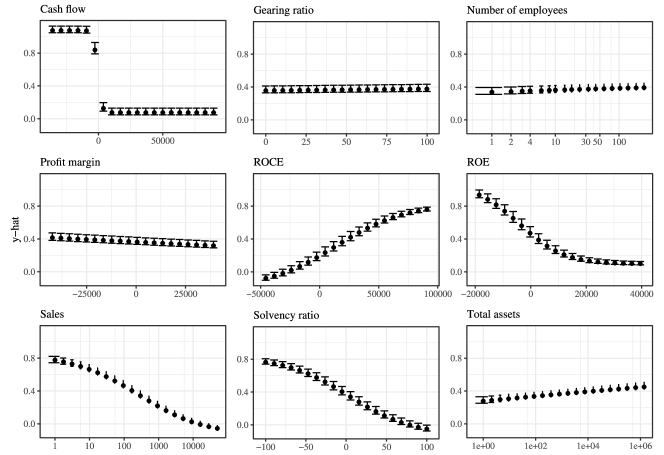
(a) a

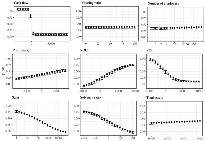
(b) b

Figure 1: Accumulated Local Effects of the LR (a) and Probit (b) models with superimposed bootstrap 5%-95% confidence intervals. The ALEs for Sales, Total Assets and Number of Employees are calculated on log-transformation of the variables but depicted on anti-log values to enhance readability.

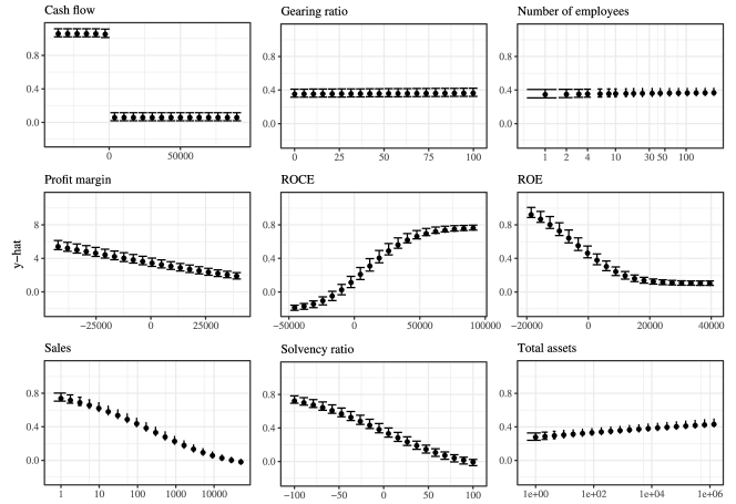
Figure 2: Accumulated Local Effects of the BGEVA model with superimposed bootstrap 5%-95% confidence intervals. The ALEs for Sales, Total Assets and Number of Employees are calculated on log-transformation of the variables but depicted on anti-log values to enhance readability.

The picture changes when it comes to black-box models. Global Shapley values indicate (figure 3) that both FANN and XGBoost predictions are influenced mainly by Profit margin. This outcome is further clarified by the average change in the model output corresponding to increasing values of the variable, represented by ALEs (figure 4). The ALEs of either model show a downward sharp jump in the probability of default when moving from negative to positive values of Profit margin, with no further decrease in the probability of default as the ratio increases, revealing a clearly decreasing effect of this ratio on the probability of default, as previously found by Altman et al. (2010), Andreeva et al. (2016) and Petropoulos et al. (2019).

The negative impact of Sales, already emerged in the white-box models, is confirmed to a minor extent by both FANN and XGBoost (second and third important variable respectively according to Shapley values). However, the pattern of the estimated default probabilities for Sales is unlike: a smooth path with no evident plateauing effect in FANN and a first sudden decrease around 100.000 euros and a second drop around 316.000 euros in XGBoost.

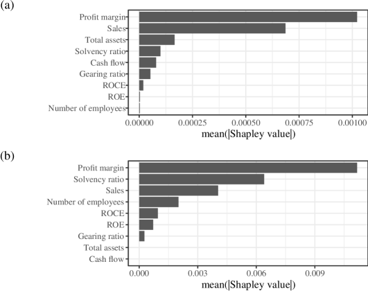
Figure 3: Global Shapley values for the Feedforward Artificial Neural Network model (a) and the XGBoost model (b)

A remarkable difference with respect to the white-box models are the sways of Total assets and the Number of employees. Total assets is the third important variable for FANN according to the Shapley values and seems to increase the probability of default judging from ALEs. On the contrary, the variable does not appear important in the prediction by XGBoost (Shapley value close to 0 and flat ALE). A positive impact of Total assets on the probability of default is anomalous, though shared by other scholars (Andreeva et al., 2016), in the light of our descriptive statistics and referring to the literature on firm demography, where exit is usually associated to less tangible assets (Michala et al., 2013). This effect could be associated to the same found by other authors in the credit scoring literature. In that case a non-linear behaviour could be explained from the fact that creditors do pursue firms with larger assets with the hope to get back the money they have lent, whereas firms with low tangible assets are less worth being pursued (Altman et al., 2010; El Kalak and Hudson, 2016).

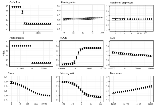
(a) a

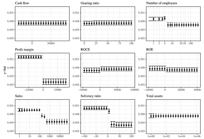
(b) b

Figure 4: Accumulated Local Effects of the FANN (a) and XGBoost (b) with related bootstrap 5%-95% confidence intervals. The ALEs for Sales, Total Assets and Number of Employees are calculated on log-transformation of the variables but depicted on anti-log values to enhance interpretability.

A somewhat opposite situation regards the Number of employees: FANN attributes scarce weight to this variable whereas XGBoost highlights its moderate impact (fourth important variable in the Shapley values) and a decrease in the probability of default around 5 employees. The XGBoost algorithm seems therefore able to capture separate and concordant effects of two variables of firm size, one on the input and the other on the output side, in decreasing the probability of default, contrary to other empirical applications (Andreeva et al., 2016).

The Solvency ratio behaves similarly to Sales, for which the XGBoost shows a plateauing effect after 0 that the FANN does not point out. However, its importance, measured by the Shapley values, differs between the two algorithms since it is the second most relevant variable for XGBoost and the fourth relevant variable in the FANN.

The Cash flow, the third variable impacting on default according to white-box models, keeps a negative sign also in FANN, while it is not relevant into the XGBoost model (as in Michala et al. (2013)). The Gearing ratio, ROCE and ROE are of a little consequence for XGBoost output and even less for the FANN according to the Shapley values and to overlapping bootstrap confidence intervals in Figure 4, but for the FANN’s ALEs plot that displays ROCE (however small its importance) as enhancing the probability of default, which is in line with part of the literature (Calabrese et al. (2016) pointed out ROCE’s positive effect). Another part of the literature instead found it non-significant (Ahelegbey et al., 2019; Giudici et al., 2020).

To summarize, blurry effects of one or more variables are encountered for the FANN model (Total assets and ROCE) and for all the white-box models (ROCE for all of them, Profit margin only for the Probit). Considering the prominent roles assigned by FANN to both Sales and Total assets, it seems that these two variables compensate one another in the wrong way, resulting in a the lowest correct classification of defaulted firms among the competing models.

An interesting puzzle remains regarding the completely different ranking in the importance of variables according to white versus black-box models. Keeping performance in mind, we should consider what emerges from the interpretation of the XGBoost output, attributing the highest sensitivity achieved to an evaluation of the interplay among the variables which ends up more effective in predicting default.

6 Conclusions

Making an AI system interpretable allows external observers to understand its working and meaning, with the non-negligible consequence of making it usable in the practice: when a firm (or a customer) applies for a credit line, it has the right to know the eventual reasons for a refusal. AI driven decisions must be explained - as much as possible- to and understood by those directly and indirectly affected, in order to allow for contesting of such decisions. This issue has become extremely relevant since both academicians and practitioners has progressively embraced ML modelling of firm default due to excellent performances (Ciampi et al., 2021) and, concurrently, Institutions have started to question the trustworthiness of - and set boundaries for - a safe use of AI in the interest of all involved (European Commission, 2019b). On the same time, using AI methods might grant larger amounts of credit and result in lower default rates (Moscatelli et al., 2020).

Here we contribute to the literature on SMEs default by showing that the good performances in classification tasks obtained through ML models can and should be accompanied by a clear interpretation of the role and type of effect played by the variables involved. Our approach belongs to the post-hoc model-agnostic interpretability methods that, differently from the ante-hoc techniques, enable the comparison among white and black-boxes on a common ground.

Using a collection of relevant accounting indicators, widely employed in the literature, for all the Italian SMEs available in the dataset Orbis by BvD for 2016, we have supplied an accurate prediction of default in 2017. Thanks to our research design, caring for imbalance among classes and cross-validation to select the most performing rules, we have achieved fair rates of correct classifications for all the models involved. However, focusing in particular on the correct rate of default classification, the XGBoost algorithm prevails over three white-box models and over the alternative ML model FANN.

Interpretability was provided by means of Shapley values and ALEs, two recent model-agnostic techniques which measure the relative importance of the predictors and shape the predictor-outcome relationship respectively. The analysis of the XGBoost ALEs reveals that such complex models capture highly non-linear patterns as the effects of sales on the probability of default, account for separate effects of correlated measures and suggest also non-trivial risky thresholds: something that was not completely grasped by any standard discriminant models.

We think that the examination of ALEs for models which are already ante-hoc interpretable in the traditional scheme of statistical significance is quite revealing, both methodologically and empirically speaking. The latter models’ ALEs permits to add different shades to the variables’ effects with respect to the standard parameter-pvalues’ paradigm. Finally, the assessment of ALEs’ variability is fundamental to check the output robustness and to evaluate the soundness of results.

With this paper we have showed that, assumed interpretability to be crucial for building and maintaining users’ trust in AI systems, their -potential- superiority in classification tasks needs not be anymore an alibi to hide the underlying mechanisms in black-boxes.

The relevancy of this approach could become definitely more important for default prediction based on alternative sources of data, such as web-scraped information, whose dimensionality and complexity require the power of ML models and whose interpretability is even more puzzling. This, as well as applications to a more extensive basket of traditional predictors, might represent a good ground for further research.

7 Acknowledgements

This project was possible thanks to the MIUR’s project “Department of Excellence” and the Department of Department of Economics, Management and Statistics Big Data Lab which provided the virtual machine on which the analysis was carried out.

References

- Abel-Koch et al. (2018) Abel-Koch, J., Acevedo, M., Bruno, C., del Bufalo, G., Ehmer, P., Gazaniol, A., Thornary, B., 2018. Internationalisation of European SMEs–Taking Stock and Moving Ahead, Research Paper by Bpi France, British Business Bank, Cassa Depositi e Prestiti SpA, Instituto de Crédito Oficial, KfW Bankengruppe. URL: https://www.kfw.de/PDF/Download-Center/Konzernthemen/Research/PDF-Dokumente-Studien-und-Materialien/Internationalisation-of-European-SMEs.pdf. (Last accessed 2021.07.22).
- Ahelegbey et al. (2019) Ahelegbey, D.F., Giudici, P., Hadji-Misheva, B., 2019. Latent factor models for credit scoring in P2P systems. Physica A: Statistical Mechanics and its Applications 522, 112–121.
- Alfaro et al. (2008) Alfaro, E., García, N., Gámez, M., Elizondo, D., 2008. Bankruptcy forecasting: An empirical comparison of adaboost and neural networks. Decision Support Systems 45, 110–122.
- Alonso and Carbó (2020) Alonso, A., Carbó, J.M., 2020. Machine learning in credit risk: measuring the dilemma between prediction and supervisory cost. Documentos de Trabajo/Banco de España, 2032 .
- Altman and Sabato (2007) Altman, E.I., Sabato, G., 2007. Modelling credit risk for SMEs: Evidence from the US market. Abacus 43, 332–357.
- Altman et al. (2010) Altman, E.I., Sabato, G., Wilson, N., 2010. The value of non-financial information in small and medium-sized enterprise risk management. J. Credit Risk 6, 1–33.
- Andreeva et al. (2016) Andreeva, G., Calabrese, R., Osmetti, S.A., 2016. A comparative analysis of the UK and Italian small businesses using generalised extreme value models. European Journal of Operational Research 249, 506–516.
- Andries et al. (2018) Andries, A.M., Marcu, N., Oprea, F., Tofan, M., 2018. Financial infrastructure and access to finance for european SMEs. Sustainability 10, 3400.
- Apley and Zhu (2020) Apley, D.W., Zhu, J., 2020. Visualizing the effects of predictor variables in black box supervised learning models. Journal of the Royal Statistical Society: Series B (Statistical Methodology) 82, 1059–1086.
- Arrieta et al. (2020) Arrieta, A.B., Díaz-Rodríguez, N., Del Ser, J., Bennetot, A., Tabik, S., Barbado, A., García, S., Gil-López, S., Molina, D., Benjamins, R., et al., 2020. Explainable Artificial Intelligence (XAI): Concepts, taxonomies, opportunities and challenges toward responsible AI. Information Fusion 58, 82–115.
- Baesens et al. (2021) Baesens, B., Höppner, S., Ortner, I., Verdonck, T., 2021. robROSE: A robust approach for dealing with imbalanced data in fraud detection. Statistical Methods & Applications doi:10.1007/s10260-021-00573-7.
- Baesens et al. (2003) Baesens, B., Van Gestel, T., Viaene, S., Stepanova, M., Suykens, J., Vanthienen, J., 2003. Benchmarking state-of-the-art classification algorithms for credit scoring. Journal of the Operational Research Society 54, 627–635.
- Bank of England (2019) Bank of England, 2019. Machine learning in UK financial services. Technical Report.
- Bellandi et al. (2020) Bellandi, M., Lombardi, S., Santini, E., 2020. Traditional manufacturing areas and the emergence of product-service systems: The case of Italy. Journal of Industrial and Business Economics 47, 311–331.
- Bellotti et al. (2021) Bellotti, A., Brigo, D., Gambetti, P., Vrins, F., 2021. Forecasting recovery rates on non-performing loans with machine learning. International Journal of Forecasting 37, 428–444.
- Breeden (2020) Breeden, J.L., 2020. Survey of Machine Learning in Credit Risk (May 30, 2020). Available at http://dx.doi.org/10.2139/ssrn.3616342.
- Bussmann et al. (2021) Bussmann, N., Giudici, P., Marinelli, D., Papenbrock, J., 2021. Explainable machine learning in credit risk management. Computational Economics 57, 203–216.
- Calabrese et al. (2016) Calabrese, R., Marra, G., Angela Osmetti, S., 2016. Bankruptcy prediction of small and medium enterprises using a flexible binary generalized extreme value model. Journal of the Operational Research Society 67, 604–615.
- Calabrese and Osmetti (2013) Calabrese, R., Osmetti, S.A., 2013. Modelling small and medium enterprise loan defaults as rare events: the generalized extreme value regression model. J. Appl. Stat. 40, 1172–1188.
- Chen and Guestrin (2016) Chen, T., Guestrin, C., 2016. XGBoost: A Scalable Tree Boosting System, in: Proceedings of the 22nd ACM SIGKDD International Conference on Knowledge Discovery and Data Mining, ACM, San Francisco California USA. pp. 785–794.
- Ciampi (2015) Ciampi, F., 2015. Corporate governance characteristics and default prediction modeling for small enterprises. an empirical analysis of Italian firms. Journal of Business Research 68, 1012–1025.
- Ciampi et al. (2021) Ciampi, F., Giannozzi, A., Marzi, G., Altman, E.I., 2021. Rethinking SME default prediction: a systematic literature review and future perspectives. Scientometrics , 1–48.
- Ciampi and Gordini (2013) Ciampi, F., Gordini, N., 2013. Small enterprise default prediction modeling through artificial neural networks: An empirical analysis of Italian small enterprises. Journal of Small Business Management 51, 23–45.
- Ciampi et al. (2009) Ciampi, F., Vallini, C., Gordini, N., Benvenuti, M., 2009. Are Credit Scoring Models Able to Predict Small Enterprise Default? Statistical Evidence from Italian Small Enterprises. International Journal of Business & Economics 8, 3–18.
- Cornille et al. (2019) Cornille, D., Rycx, F., Tojerow, I., 2019. Heterogeneous effects of credit constraints on SMEs’ employment: Evidence from the European sovereign debt crisis. Journal of Financial Stability 41, 1–13.
- Davison and Kuonen (2002) Davison, A.C., Kuonen, D., 2002. An Introduction to the Bootstrap with Applications in R. Statistical Computing and Graphics Newsletter , 6.
- Doran et al. (2017) Doran, D., Schulz, S., Besold, T.R., 2017. What does explainable AI really mean? A new conceptualization of perspectives. arXiv:1710.00794.
- Doshi-Velez and Kim (2017) Doshi-Velez, F., Kim, B., 2017. Towards a rigorous science of interpretable machine learning. arXiv:1702.08608.
- Du et al. (2019) Du, M., Liu, N., Hu, X., 2019. Techniques for interpretable machine learning. Communications of the ACM 63, 68--77.
- El Kalak and Hudson (2016) El Kalak, I., Hudson, R., 2016. The effect of size on the failure probabilities of SMEs: An empirical study on the US market using discrete hazard model. International Review of Financial Analysis 43, 135--145.
- EU (2003) EU, 2003. Commission Recommendation of 6 May 2003 Concerning the Definition of Micro, Small and Medium-Sized Enterprises (Text with EEA Relevance) (Notified under Document Number C(2003) 1422). Technical Report 32003H0361.
- European Banking Authority (2020) European Banking Authority, 2020. EBA Report on Big Data and Advanced Analytics. Technical Report.
- European Commission (2019a) European Commission, 2019a. Annual Report on European SMEs 2018/2019. Technical Report.
- European Commission (2019b) European Commission, 2019b. Ethics guidelines for trustworthy AI. Technical Report.
- Eurostat (2018) Eurostat, 2018. Relative importance of Manufacturing (NACE Section C), EU, 2018.
- Fantazzini and Figini (2009) Fantazzini, D., Figini, S., 2009. Random survival forests models for SME credit risk measurement. Methodology and Computing in Applied Probability 11, 29--45.
- Friedman (1991) Friedman, J.H., 1991. Multivariate Adaptive Regression Splines. The Annals of Statistics 19, 1--67.
- Friedman (2001) Friedman, J.H., 2001. Greedy function approximation: A gradient boosting machine. The Annals of Statistics 29, 1189--1232.
- Geng et al. (2015) Geng, R., Bose, I., Chen, X., 2015. Prediction of financial distress: An empirical study of listed chinese companies using data mining. European Journal of Operational Research 241, 236--247.
- Giudici et al. (2020) Giudici, P., Hadji-Misheva, B., Spelta, A., 2020. Network based credit risk models. Quality Engineering 32, 199--211.
- Goldstein et al. (2015) Goldstein, A., Kapelner, A., Bleich, J., Pitkin, E., 2015. Peeking Inside the Black Box: Visualizing Statistical Learning With Plots of Individual Conditional Expectation. Journal of Computational and Graphical Statistics 24, 44--65.
- Gong and Kim (2017) Gong, J., Kim, H., 2017. RHSBoost: Improving classification performance in imbalance data. Computational Statistics & Data Analysis 111, 1--13.
- Gordini (2014) Gordini, N., 2014. A genetic algorithm approach for SMEs bankruptcy prediction: Empirical evidence from Italy. Expert Systems with Applications 41, 6433--6445.
- Guidotti et al. (2018) Guidotti, R., Monreale, A., Ruggieri, S., Turini, F., Giannotti, F., Pedreschi, D., 2018. A survey of methods for explaining black box models. ACM computing surveys (CSUR) 51, 1--42.
- Gupta et al. (2018) Gupta, J., Gregoriou, A., Ebrahimi, T., 2018. Empirical comparison of hazard models in predicting SMEs failure. Quantitative Finance 18, 437--466.
- Gupta et al. (2015) Gupta, J., Gregoriou, A., Healy, J., 2015. Forecasting bankruptcy for SMEs using hazard function: To what extent does size matter? Review of Quantitative Finance and Accounting 45, 845--869.
- Hand (2009) Hand, D.J., 2009. Measuring classifier performance: A coherent alternative to the area under the ROC curve. Machine Learning 77, 103--123.
- Hand and Anagnostopoulos (2013) Hand, D.J., Anagnostopoulos, C., 2013. When is the area under the receiver operating characteristic curve an appropriate measure of classifier performance? Pattern Recognition Letters 34, 492--495.
- Haykin (1999) Haykin, S.S., 1999. Neural Networks: A Comprehensive Foundation. 2nd ed ed., Prentice Hall, Upper Saddle River, N.J.
- Hechtlinger (2016) Hechtlinger, Y., 2016. Interpretation of Prediction Models Using the Input Gradient. arXiv:1611.07634.
- High-Level Expert Group on Artificial Intelligence, European Commission (2020) High-Level Expert Group on Artificial Intelligence, European Commission, 2020. The Assessment List for Trustworthy Artificial Intelligence. Technical Report.
- Holmes et al. (2010) Holmes, P., Hunt, A., Stone, I., 2010. An analysis of new firm survival using a hazard function. Applied Economics 42, 185--195.
- Institute of International Finance (2019) Institute of International Finance, 2019. Machine learning in credit risk. Technical Report. Institute of International Finance.
- Institute of International Finance (2020) Institute of International Finance, 2020. Machine Learning Governance Summary Report. Summary Report. Institute of International Finance.
- Jabeur et al. (2021) Jabeur, S.B., Gharib, C., Mefteh-Wali, S., Arfi, W.B., 2021. Catboost model and artificial intelligence techniques for corporate failure prediction. Technological Forecasting and Social Change 166, 120658.
- James et al. (2013) James, G., Witten, D., Hastie, T., Tibshirani, R. (Eds.), 2013. An Introduction to Statistical Learning: With Applications in R. Number 103 in Springer Texts in Statistics, Springer, New York.
- du Jardin (2016) du Jardin, P., 2016. A two-stage classification technique for bankruptcy prediction. European Journal of Operational Research 254, 236--252.
- Jones et al. (2015) Jones, S., Johnstone, D., Wilson, R., 2015. An empirical evaluation of the performance of binary classifiers in the prediction of credit ratings changes. Journal of Banking & Finance 56, 72--85.
- Jones and Wang (2019) Jones, S., Wang, T., 2019. Predicting private company failure: A multi-class analysis. Journal of International Financial Markets, Institutions and Money 61, 161--188.
- Kim and Sohn (2010) Kim, H.S., Sohn, S.Y., 2010. Support vector machines for default prediction of SMEs based on technology credit. European Journal of Operational Research 201, 838--846.
- Kou et al. (2021) Kou, G., Xu, Y., Peng, Y., Shen, F., Chen, Y., Chang, K., Kou, S., 2021. Bankruptcy prediction for SMEs using transactional data and two-stage multiobjective feature selection. Decision Support Systems 140, 113429.
- Laitinen and Gin Chong (1999) Laitinen, E.K., Gin Chong, H., 1999. Early-warning system for crisis in SMEs: Preliminary evidence from Finland and the UK. Journal of Small Business and Enterprise Development 6, 89--102.
- Lessmann et al. (2015) Lessmann, S., Baesens, B., Seow, H.V., Thomas, L.C., 2015. Benchmarking state-of-the-art classification algorithms for credit scoring: An update of research 247, 124--136.
- Liberati et al. (2017) Liberati, C., Camillo, F., Saporta, G., 2017. Advances in credit scoring: combining performance and interpretation in kernel discriminant analysis. Advances in Data Analysis and Classification 11, 121--138.
- Lin et al. (2012) Lin, S.M., Ansell, J., Andreeva, G., 2012. Predicting default of a small business using different definitions of financial distress. Journal of the Operational Research Society 63, 539--548.
- Lipton (2018) Lipton, Z.C., 2018. The mythos of model interpretability: In machine learning, the concept of interpretability is both important and slippery. Queue 16, 31--57.
- Lundberg and Lee (2017) Lundberg, S., Lee, S.I., 2017. A Unified Approach to Interpreting Model Predictions, in: Advances in Neural Information Processing Systems, Curran Associates Inc., Long Beach California, USA. pp. 4765--4774.
- Mai et al. (2019) Mai, F., Tian, S., Lee, C., Ma, L., 2019. Deep learning models for bankruptcy prediction using textual disclosures. European Journal of Operational Research 274, 743--758.
- Michala et al. (2013) Michala, D., Grammatikos, T., Filipe, S.F., 2013. Forecasting Distress in European SME Portfolios. EIF Working Paper 2013/17. European Investment Fund (EIF). Luxembourg.
- Modina and Pietrovito (2014) Modina, M., Pietrovito, F., 2014. A default prediction model for Italian SMEs: the relevance of the capital structure. Applied Financial Economics 24, 1537--1554.
- Montavon et al. (2018) Montavon, G., Samek, W., Müller, K.R., 2018. Methods for interpreting and understanding deep neural networks. Digital Signal Processing 73, 1--15.
- Moscatelli et al. (2020) Moscatelli, M., Parlapiano, F., Narizzano, S., Viggiano, G., 2020. Corporate default forecasting with machine learning. Expert Systems with Applications 161, 113567.
- Nehrebecka (2018) Nehrebecka, N., 2018. Predicting the default risk of companies. comparison of credit scoring models: Logit vs support vector machines. Econometrics 22, 54--73.
- Oliveira et al. (2017) Oliveira, M.D., Ferreira, F.A., Pérez-Bustamante Ilander, G.O., Jalali, M.S., 2017. Integrating cognitive mapping and mcda for bankruptcy prediction in small-and medium-sized enterprises. Journal of the Operational Research Society 68, 985--997.
- Petropoulos et al. (2019) Petropoulos, A., Siakoulis, V., Stavroulakis, E., Klamargias, A., 2019. A robust machine learning approach for credit risk analysis of large loan-level datasets using deep learning and extreme gradient boosting, in: IFC Bulletins Chapters. Bank for International Settlements. volume 50.
- Psillaki et al. (2010) Psillaki, M., Tsolas, I.E., Margaritis, D., 2010. Evaluation of credit risk based on firm performance. European Journal of Operational Research 201, 873--881.
- Ribeiro et al. (2016a) Ribeiro, M.T., Singh, S., Guestrin, C., 2016a. Model-agnostic interpretability of machine learning. arXiv:1606.05386.
- Ribeiro et al. (2016b) Ribeiro, M.T., Singh, S., Guestrin, C., 2016b. "Why should I trust you?" Explaining the predictions of any classifier, in: Proceedings of the 22nd ACM SIGKDD International Conference on Knowledge Discovery and Data Mining, pp. 1135--1144.
- Ribeiro et al. (2018) Ribeiro, M.T., Singh, S., Guestrin, C., 2018. Anchors: High-Precision Model-Agnostic Explanations, in: AAAI, Association for the Advancement of Artificial Intelligence. pp. 1527--1535.
- Santos et al. (2018) Santos, M.S., Soares, J.P., Abreu, P.H., Araujo, H., Santos, J., 2018. Cross-Validation for Imbalanced Datasets: Avoiding Overoptimistic and Overfitting Approaches [Research Frontier]. IEEE Computational Intelligence Magazine 13, 59--76.
- Shapley (1953) Shapley, L.S., 1953. 17. A Value for n-Person Games, in: Kuhn, H.W., Tucker, A.W. (Eds.), Contributions to the Theory of Games (AM-28), Volume II. Princeton University Press, pp. 307--318. doi:10.1515/9781400881970-018.
- Sigrist and Hirnschall (2019) Sigrist, F., Hirnschall, C., 2019. Grabit: Gradient tree-boosted Tobit models for default prediction. Journal of Banking & Finance 102, 177--192.
- Sohn and Kim (2007) Sohn, S.Y., Kim, H.S., 2007. Random effects logistic regression model for default prediction of technology credit guarantee fund. European Journal of Operational Research 183, 472--478.
- Stevenson et al. (2021) Stevenson, M., Mues, C., Bravo, C., 2021. The value of text for small business default prediction: A Deep Learning approach. European Journal of Operational Research 295, 758--771.
- Su et al. (2021) Su, C.H., Tu, F., Zhang, X., Shia, B.C., Lee, T.S., 2021. A Ensemble Machine Learning Based System for Merchant Credit Risk Detection in Merchant MCC Misuse. Journal of Data Science 17, 81--106.
- Succurro et al. (2014) Succurro, M., Mannarino, L., et al., 2014. The Impact of Financial Structure on Firms’ Probability of Bankruptcy: A Comparison across Western Europe Convergence Regions. Regional and Sectoral Economic Studies 14, 81--94.
- West (2000) West, D., 2000. Neural network credit scoring models. Computers & Operations Research 27, 1131--1152.
- West et al. (2005) West, D., Dellana, S., Qian, J., 2005. Neural network ensemble strategies for financial decision applications. Computers & Operations Research 32, 2543--2559.
- Xu and Liang (2001) Xu, Q.S., Liang, Y.Z., 2001. Monte Carlo Cross Validation. Chemometrics and Intelligent Laboratory Systems 56, 1--11.
- Yıldırım et al. (2021) Yıldırım, M., Okay, F.Y., Özdemir, S., 2021. Big data analytics for default prediction using graph theory. Expert Systems with Applications 176, 114840.
- Zhang et al. (2015) Zhang, L., Hu, H., Zhang, D., 2015. A credit risk assessment model based on SVM for small and medium enterprises in supply chain finance. Financial Innovation 1, 1--21.