GRP-FED: Addressing Client Imbalance in Federated Learning via Global-Regularized Personalization

Abstract

Since data is presented long-tailed in reality, it is challenging for Federated Learning (FL) to train across decentralized clients as practical applications. We present Global-Regularized Personalization (GRP-FED) to tackle the data imbalanced issue by considering a single global model and multiple local models for each client. With adaptive aggregation, the global model treats multiple clients fairly and mitigates the global long-tailed issue. Each local model is learned from the local data and aligns with its distribution for customization. To prevent the local model from just overfitting, GRP-FED applies an adversarial discriminator to regularize between the learned global-local features. Extensive results show that our GRP-FED improves under both global and local scenarios on real-world MIT-BIH and synthesis CIFAR-10 datasets, achieving comparable performance and addressing client imbalance.

1 Introduction

Federated Learning (FL) is a distributed learning algorithm that trains models across multiple decentralized clients and keeps data private simultaneously (McMahan et al., 2017; Konečnỳ et al., 2016). One of the issues in FL is the distinct distributions where decentralized data is diverse due to different properties over each client (Kairouz et al., 2019; Liang et al., 2020; Deng et al., 2020; Li et al., 2019).

Figure 1: The client imbalanced issue in the real-world MIT-BIH dataset. (a) visualizes the client distribution as each client point via t-SNE; (b) plots the class distribution of the global and selected clients; (c) presents the performance (Macro-F1) of FedAvg on the entire test (global) or specific clients (local).

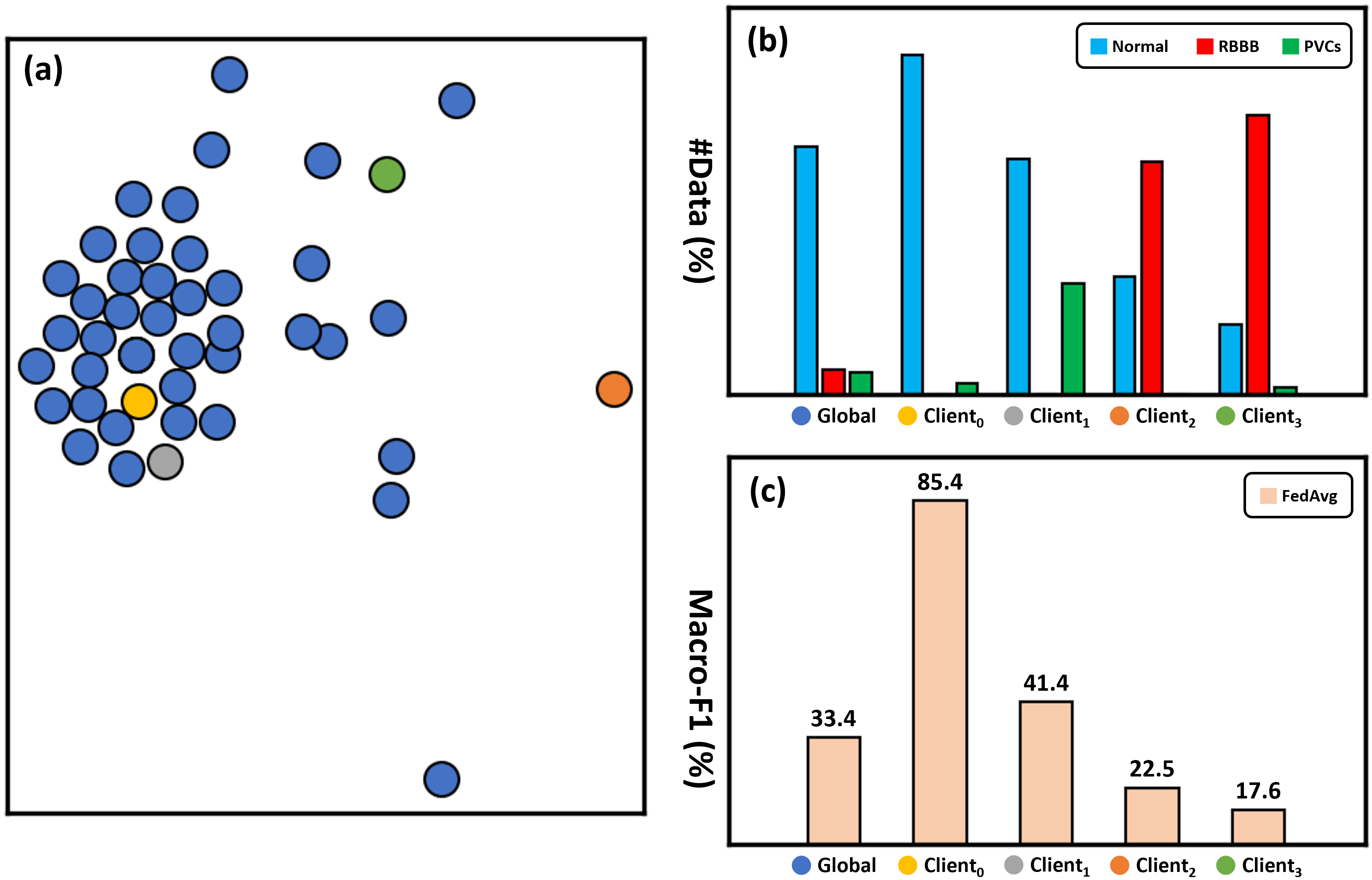
In the real world, data is inevitably long-tailed (Yang & Xu, 2020). Fig. 1 illustrates the data distribution of MIT-BIH (Goldberger et al., 2000), a real-world Electrocardiography (ECG) dataset for medical diagnosis. Each patient, which may have different arrhythmia issues over several ECGs, is viewed as a client under the FL setting. Fig. 1(a) visualizes the client distribution as each client point using t-SNE (Maaten & Hinton, 2008). It shows that the global distribution of clients is non-uniformly, where some clients are scattered and far away. Fig. 1(b) plots the class distribution of data from clients, which shares distinct distributions and provides different class data.

FedAvg (McMahan et al., 2017) is a classic FL algorithm where a single model tries to fit among clients by averaging the parameters from local training. Fig. 1(c) presents the Macro-F1 score of FedAvg for global and client-based (local) testing. Since conducting all clients equally, FedAvg ignores the various data distributions between clients, making the poor performance on the global test. Furthermore, FedAvg is easily dominated by major clients but gives up remaining clients, where the F1 score drops drastically on them. Fig. 1 shows this imbalanced issue that makes applying FL to practical applications challenging.

Even if encouraging worse clients to focus on global fairness (Mohri et al., 2019; Li et al., 2019), the performance gap between global and local tests is still significant (Jiang et al., 2019), which indicates that personalization is crucial in FL. The local training (Fallah et al., 2020; Khodak et al., 2019; Liang et al., 2020; Dinh et al., 2020) adopts personalization by training part of local models only on client data as customization. However, the local models, which directly minimize the local error, suffer from overfitting and lose the discrimination of those minor local classes.

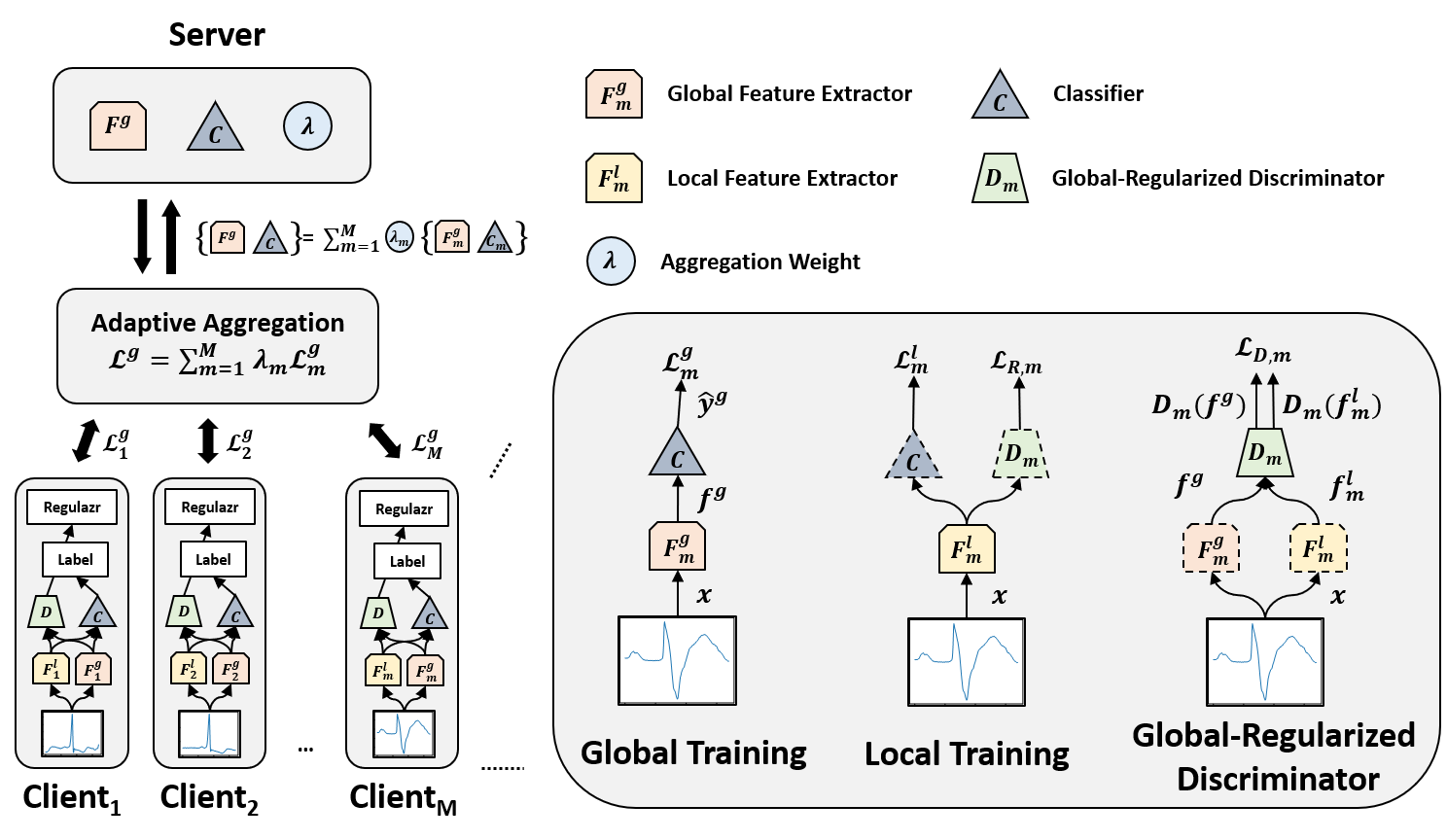
In this paper, we introduce Global-Regularized Personalization (GRP-FED) to address client imbalance in FL. As shown in Fig. 2, GRP-FED contains a single global model and local models for each client to consider global fairness and local personalization. Since each client provides different amounts and aspects of class data, our GRP-FED presents Adaptive Aggregation to adaptively adjust the weight of each client and aggregate as a fairer global model. To do personalization, local models are only trained on the specific data for each client. In case of being customizing but overfitting, we present the Global-Regularized Discriminator (D) to distinguish that an extracted feature is from the global or the local model. By jointly optimizing to fool D, local models learn the specific distribution for each client and the general global feature to avoid overfitting.

We conduct the evaluation on real-world MIT-BIH (Goldberger et al., 2000) and synthesis CIFAR-10 (Krizhevsky & Hinton, 2009) datasets under FL setting. The experimental results show that our GRP-FED can improve both global and local tests. Furthermore, the proposed global-regularized discriminator addresses local overfitting effectively. In summary, our contributions are three-fold:

• We present GRP-FED to simultaneously consider global fairness and local personalization for Federated Learning;

• The proposed adaptively-aggregated global model and customized local models gain improvement under both global and local scenarios;

• Extensive ablation studies on both real-world MIT-BIH and synthesis CIFAR-10 show that GRP-FED achieves better performance and deals with client imbalance.

Figure 2: An overview of Global-Regularized Personalization (GRP-FED) for the federated learning (FL). For better global fiarness, we adopt adaptive aggregation to investigate different aspects and proportions of clients. We make each local client optimize only on their client to support personalization. In addition, the proposed global-regularized discriminator helps to prevent from overfitting.

2 Related Work

Federated Learning (FL)  Federated Learning (FL) (McMahan et al., 2017; Konečnỳ et al., 2016), where models are trained across multiple decentralized clients, aims to preserve user privacy (Li et al., 2020; Basu et al., 2019) and lower communication costs (Li et al., 2020; Basu et al., 2019). Similar to imbalanced data distribution (Hanzely & Richtárik, 2020; Khodak et al., 2019; Wang et al., 2021; Duan et al., 2020), we investigate the global model used for all and new data and local models that are customized and support personalization for local clients.

Global Model for FL  In FL, the global model is trained from all clients and fit the overall global distribution. FedAvg (McMahan et al., 2017) is the first to apply local SGD and build a single global model from a subset of clients. Moreover, they improve global fairness by adapting the global model better to each client (Fallah et al., 2020; Khodak et al., 2019) or treating clients with different importance weights (Mohri et al., 2019). Inspired by q-FFL (Li et al., 2019), which utilizes a constant power to tune the amount of fairness, our GRP-FED adaptively adjusts the power of loss to satisfy dynamic fairness during the global training.

Local Model for FL  The performance gap between global and local tests indicates that personalization is crucial in FL (Jiang et al., 2019). Local fine-tuning (Smith et al., 2017; Chen et al., 2020; Khodak et al., 2019; Fallah et al., 2020; Liang et al., 2020) supports personalization by training each local model only on client data. While, pFedMe (Dinh et al., 2020) argues that directly minimizing local error is prone to overfit and adopts Moreau envelopes to help decouple personalization. Different from that, our GRPFED introduces the Global-Regularized Discriminator to regularize the local feature distribution and mitigate the local overfitting issue.

3 Approach

3.1 Overview

Task Definition  Federated Learning (FL) is to learn from independent $M$ clients where client $m$ contains a local dataset $\mathcal{D}_{m}=\{(x_{0},y_{0})_{m},...,(x_{N_{m}},y_{N_{m}})_{m}\}$. $(x_{i},y_{i})_{m}$ represents the pair of $i$th data and its label where $N_{m}$ is the number of data in $\mathcal{D}_{m}$. We consider FL as classification task where $y$ is the class label of $x$. Intuitively, each client captures a different view $p(X,Y)_{m}$ of the global data distribution $p(X,Y)$. However, since each client provides $\mathcal{D}$ with distinct distributions in real world, FL easily suffers from the client imbalance under practical applications.

GRP-FED  To address the client imbalanced issue, we present Global-Regularized Personalization (GRP-FED) into FL. An overview of GRP-FED is illustrated in Fig. 2. For a data point $x$, the feature extractor $F$ extracts the lower-dimensional representation of $x$, and the classifier $C$ performs the output prediction $\hat{y}$. GRP-FED consists of a fair global model that applies adaptive aggregation to consider different aspects from clients, and local models to customize each client. The proposed adaptive aggregation adjusts the aggregated proportion to ensure the fairness over distinct clients. The local models do personalization, where a global-regularized discriminator prevents it from overfitting when optimizing the client data.

3.2 Global Fairness

Global Training  Global fairness aims at building a global model that can fairly cope with the global distribution over distinct clients. The global model includes the global feature extractor $F$ parameterized by $\theta^{g}_{F}$ and the classifier $C$ parameterized by $\theta_{C}$. The global training is to train the global model in each client $m$ and then aggregated as a single global model:

$$\begin{split}f^{g}_{i}&=F(x_{i};\theta^{g(t)}_{F,m}),\hat{y_{i}}=C(f^{g}_{i};\theta_{C}),\\ \mathcal{L}^{g(t)}_{m}&=\mathbb{E}_{(x_{i},y_{i})\sim\mathcal{D}_{m}}J(\hat{y}_{i},y_{i}),\\ \end{split}$$ (1)

where $f^{g}$ is the extracted global feature. $\mathcal{L}^{g}(t)$ is calculated by the loss function $J$ at time step $t$ and updates to receive $\theta^{g(t+1)}_{F,m}$. In conventional FL, FedAvg (Smith et al., 2017) considers the global model by averaging all trained global models from clients. However, under the real-world FL setting, client data is collected from different environments, scenarios, or applications. The data distribution $p(X,Y)_{m}$ from each client presents diversely, which results in poor generalization if treating them equally. To deal with the client imbalanced issue, we propose adaptive aggregation for a fairer aggregated proportion.

1:  Server:

2:  Initialize $\theta^{g}_{F}$, $\theta^{l}_{F,{\{1:M\}}}$, $\theta_{C}$, $\theta_{D,{\{1:M\}}}$, $\lambda$

3:  

4:  for $t=1~{}\text{to}~{}T$ do

5:     $S_{t}$ $\leftarrow$ randomly select $m$ clients

6:     for $m$ $\in$ $S_{t}$ do

7:       $\theta_{F_{m}}^{g(t+1)}$, $\theta_{C_{m}}^{(t+1)}$, $\mathcal{L}^{g(t+1)}_{m}$ $\leftarrow$ Client($m$, $\theta_{F}^{g(t)}$, $\theta_{C}^{(t)}$)

8:     end for

9:     

10:     $\triangleright$ Adaptive aggregation by adaptive $q$

11:     $q^{(t+1)}=q^{t}+\eta_{q}\frac{\sigma(\mathcal{L}^{g(t+1)})-\sigma(\mathcal{L}^{g(t)})}{(\sigma(\mathcal{L}^{g(t+1)})+\sigma(\mathcal{L}^{g(t)}))/2}$

12:     $\lambda_{m}=\frac{(\mathcal{L}^{g(t+1)}_{m})^{q(t+1)}}{\sum_{i=1}^{M}(\mathcal{L}^{g(t+1)}_{i})^{q(t+1)}}$

13:     $\{\theta_{F}^{g(t+1)},\theta_{C}^{g(t+1)}\}=\sum_{i=1}^{M}\lambda_{i}\{\theta_{F,i}^{g(t+1)},\theta_{C,i}^{g(t+1)}\}$

14:  end for

15:  

16:  Client($m$, $\theta^{g}_{F}$, $\theta_{C}$):

17:  $\theta^{g}_{F,m},\theta_{C,m}$ $\leftarrow$ $\theta^{g}_{F},\theta_{C}$

18:  for $r=1~{}\text{to}~{}R$ do

19:     $\mathcal{B}$ $\leftarrow$ batches ($\mathcal{D}_{m}$)

20:     for batch ($x$, $y$) $\in$ $\mathcal{B}$ do

21:       $\triangleright$ Run with the global model

22:       $\hat{y}^{g}=C(F(x;\theta^{g}_{F,m});\theta_{C,m})$

23:       $\mathcal{L}^{g}_{m}=J(\hat{y}^{g},y)$

24:       $\theta^{g}_{F,m}=\theta^{g}_{F,m}-\eta\nabla_{\theta^{g}_{F,m}}\mathcal{L}^{g}_{m}$

25:       $\theta^{g}_{C,m}=\theta^{g}_{C,m}-\eta\nabla_{\theta^{g}_{C,m}}\mathcal{L}^{g}_{m}$

26:       

27:       $\triangleright$ Run with the local model

28:       $\hat{y}^{l}=C(F(x;\theta^{l}_{F,m});\theta_{C})$

29:       $\mathcal{L}^{l}_{m}=J(\hat{y}^{l},y)$

30:       $\mathcal{L}_{R,m}=\log(1-D(f^{l};\theta_{D,m}))$ $\triangleright$ Update also with $D$

31:       $\theta^{l}_{F_{m}}$ $\leftarrow$ $\theta^{l}_{F_{m}}-\eta\nabla_{\theta^{l}_{F_{m}}}(\beta\mathcal{L}^{l}_{m}+(1-\beta)\mathcal{L}_{R,m})$

32:       

33:       $\triangleright$ Update $\theta_{D,m}$ with $f^{g}$ as true and $f^{l}$ as false

34:       $f^{g},f^{l}=F(x;\theta^{g}_{F}),F(x;\theta^{l}_{F,m})$

35:       $\mathcal{L}_{D,m}=\log(1-D(f^{g};\theta_{D,m}))+\log(D(f^{l};\theta_{D,m}))$

36:       $\theta_{D,m}$ $\leftarrow$ $\theta_{D,m}-\eta\nabla_{\theta_{D,m}}\mathcal{L}_{D,m}$

37:     end for

38:  end for

39:  return $\theta^{g}_{F,m}$, $\theta_{C,m}$, $\mathcal{L}^{g}_{m}$ to server

Algorithm 1 GRP-FED, $\eta$: learning rate, $J$: loss function

Adaptive Aggregation  q-FFL (Li et al., 2019) adopts a constant power $q$ that tunes the amount of fairness. However, the training process for FL can be dynamic over distinct clients, where a fixed power of loss is difficult to satisfy the expected fairness under all situations. To overcome this issue, we present adaptive aggregation and consider a dynamic $q$ to adaptively adjusts for better fairness. We treat fairness as the standard deviation ($\sigma$) of the global training loss $\mathcal{L}^{g}$ in all clients. If $\sigma$ is high, the global training loss is quite different and the global model may suffer from client imbalance. Therefore, we adjust the loss of power $q$:

$$q^{(t+1)}=q^{t}+\eta_{q}\frac{\sigma(\mathcal{L}^{g(t+1)})-\sigma(\mathcal{L}^{g(t)})}{(\sigma(\mathcal{L}^{g(t+1)})+\sigma(\mathcal{L}^{g(t)}))/2}.$$ (2)

Otherwise, if the fairness becomes relatively fairer, we should decrease $q$ for more robust training. Finally, we acquire the new global model by aggregating all trained global models, weighted by the global training loss $\mathcal{L}^{g}$ and the adaptive power $q$:

$$\begin{split}\lambda_{m}&=\frac{(\mathcal{L}^{g(t+1)}_{m})^{q(t+1)}}{\sum_{i=1}^{M}(\mathcal{L}^{g(t+1)}_{i})^{q(t+1)}},\\ \{\theta_{F}^{g(t+1)},\theta_{C}^{g(t+1)}\}&=\sum_{i=1}^{M}\lambda_{i}\{\theta_{F,i}^{g(t+1)},\theta_{C,i}^{g(t+1)}\}.\end{split}$$ (3)

In this way, we can adaptively adjust to satisfy the dynamic fairness during the global training by considering the standard deviation of the global training loss over all clients.

3.3 Local Personalization

Local Training  Apart from a single global model, since each client is collected from different sources and under various usages, local models that support personalization are also crucial. The local training is to train each local model only with the data in client $m$ for personalization:

$$\begin{split}f^{l}_{i}&=F(x_{i};\theta^{l(t)}_{F,m}),\hat{y_{i}}=C(f^{l}_{i};\theta_{C}),\\ \mathcal{L}^{l(t)}_{m}&=\mathbb{E}_{(x_{i},y_{i})\sim\mathcal{D}_{m}}J(\hat{y}_{i},y_{i}),\\ \end{split}$$ (4)

where $f^{l}$ is the extracted personalized feature. Similar to the global training, $\theta^{l(t+1)}_{F,m}$ is updated by $\mathcal{L}^{l}$ from $J$. Thereby, we personalize the local feature $f^{l}$ in the specific client. Note that we fix the classifier $C$ with $\theta_{C,m}$ during the local training for a personalized local feature distribution.

Global-Regularized Discriminator ($D$)  After the local training, we can have the personalized feature $f^{l}$. However, since under FL, the client data distribution $p(X,Y)_{m}$ is far from global $p(X,Y)$, the learned $f^{l}$ may be just overfitting on that client but suffers from poor generalization for the global scenario. To mitigate this overfitting issue, we introduce Global-Regularized Discriminator ($D$). Each client $m$ maintains its own $D$ parameterized by $\theta_{D,m}$, which serves as a binary classifier to distinguish an extracted feature $f$ is from the global or the local feature extractor. We make the global feature $f^{g}$ by $\theta^{g}_{F}$ as the true case and the local feature $f^{l}$ by $\theta^{l}_{F,m}$ as the false case, and train $D_{m}$ as following:

$$\begin{split}f^{g}_{i}&=F(x_{i};\theta^{g}_{F}),f^{l}_{i}=F(x_{i};\theta^{l}_{F,m})\\ \mathcal{L}_{D,m}&=\mathbb{E}_{x_{i}\sim\mathcal{D}_{m}}\log(1-D(f^{g}_{i};\theta_{D,m}))+\log(D(f^{l}_{i};\theta_{D,m})),\end{split}$$

where $\theta^{g}_{F}$ and $\theta^{l}_{F,m}$ are fixed, and only $\theta_{D_{m}}$ is updated during the $D_{m}$ training. With the help of $D_{m}$, the local feature extractor $\theta^{g}_{F,m}$ can be regularized to prevent overfitting:

$$\mathcal{L}_{R,m}=\mathbb{E}_{x_{i}\sim\mathcal{D}_{m}}\log(1-D(f^{l}_{i};\theta_{D,m})).$$ (5)

This time, $\theta_{D_{m}}$ should be freeze and $\theta^{l}_{F,m}$ is optimized to fool the discriminator $D_{m}$. By updating the local training along with the global-regularized discriminator, the local feature extractor learns to personalize and imitate the global feature distribution, which can avoid client overfitting.

	MIT-BIH					CIFAR-10
Method	Global Test	Local Test	Personalization	Generalization		Global Test	Local Test	Personalization	Generalization
Local	0.075$\pm$0.009	0.140$\pm$0.001	0.933$\pm$0.005	0.076$\pm$0.001		0.214$\pm$0.022	0.290$\pm$0.005	0.396$\pm$0.009	0.235$\pm$0.003
FedAvg	0.334$\pm$0.046	0.407$\pm$0.044	0.684$\pm$0.011	0.334$\pm$0.046		0.462$\pm$0.006	0.482$\pm$0.004	0.518$\pm$0.001	0.462$\pm$0.006
AFL	0.506$\pm$0.018	0.503$\pm$0.023	0.606$\pm$0.042	0.506$\pm$0.018		0.495$\pm$0.004	0.496$\pm$0.006	0.510$\pm$0.009	0.495$\pm$0.004
q-FFL	0.551$\pm$0.034	0.534$\pm$0.006	0.602$\pm$0.033	0.551$\pm$0.001		0.563$\pm$0.003	0.530$\pm$0.007	0.510$\pm$0.009	0.563$\pm$0.003
per-FedAvg	0.378$\pm$0.030	0.424$\pm$0.022	0.799$\pm$0.004	0.310$\pm$0.024		0.525$\pm$0.021	0.490$\pm$0.014	0.550$\pm$0.012	0.453$\pm$0.017
pFedMe	0.290$\pm$0.011	0.288$\pm$0.012	0.850$\pm$0.006	0.178$\pm$0.001		0.406$\pm$0.010	0.414$\pm$0.007	0.503$\pm$0.014	0.356$\pm$0.010
LG-FedAvg	0.343$\pm$0.034	0.286$\pm$0.010	0.964$\pm$0.007	0.169$\pm$0.006		0.503$\pm$0.025	0.499$\pm$0.015	0.676$\pm$0.017	0.403$\pm$0.014
GRP-FED	0.569$\pm$0.004	0.553$\pm$0.011	0.864$\pm$0.022	0.424$\pm$0.007		0.578$\pm$0.001	0.552$\pm$0.010	0.611$\pm$0.010	0.516$\pm$0.007

Table 1: The quantitative results of our GRP-FED and baselines in the global test ($T_{g}$) and the local test ($T_{l}$), including the personalization test ($T_{p}$) and the generalization test ($T_{r}$), on both real-world MIT-BIH and synthesis CIFAR-10 datasets.

3.4 Learning of GRP-FED and Inference

The learning process of GRP-FED is presented in Algo. 1. For each round $t$, to make the federated learning stable, we follow (Smith et al., 2017) that randomly selects $m$ clients as $S_{t}$ for training. At first, the server copies global feature extractor $\theta^{g}_{F}$ and classifier $\theta_{C}$ to the clients for independent federated training. Both $\theta^{g}_{F}$ and $\theta^{C}$ are trained through data from all clients during the global training. For the local training, the local feature extractor $\theta^{l}_{F}$ is only trained by the client data and updated from the $\mathcal{L}^{l}_{m}$ to do personalization on client $m$. Also, $\theta^{l}_{F}$ is jointly trained from $\mathcal{L}_{R,m}$ to prevent overfitting. The global-regularized discriminator ($D$) $\theta_{D,m}$ then updates from $\mathcal{L}_{D,m}$ by discriminating an feature is extracted from the local or global model, where $\beta$ is the weight of loss between $\mathcal{L}^{l}_{m}$ and $\mathcal{L}_{R,m}$.

After returning all trained $\theta^{g}_{F,m}$, $\theta_{C,m}$, and global training loss $\mathcal{L}^{g}_{m}$ from each client $m$, we aggregate $\theta^{g}_{F,m}$ and $\theta^{g}_{C,m}$ as the new global model over the aggregated weight $\lambda$. $\lambda$ is updated from the adaptive power $q$ and the global training loss $\mathcal{L}^{g}$ to force investigating different proportions of clients. In total, the entire training loss $\mathcal{L}_{\text{T}}$ of GRP-FED is:

$$\scriptsize\mathcal{L}_{\text{T}}=\sum_{m\in S_{t}}\mathcal{L}^{g}_{m}+\underbrace{\sum_{m\in S_{t}}(\beta\mathcal{L}^{l}_{m}+(1-\beta)\mathcal{L}_{R,m})}_{\text{Local Personalization}}+\underbrace{\sum_{m\in S_{t}}\mathcal{L}_{D,m}}_{\text{Discriminator}}.$$

Inference  During inference, given an example $x^{\prime}$, we consider two testing types for both local and global scenario:

• local test: if $x^{\prime}$ belongs to client $m$, we apply the local model ($\theta^{l}_{F,m}$) for the best personalization;

• global test: otherwise, $x^{\prime}$ is fed to the global model ($\theta^{g}_{F}$) as an unknown example from the global distribution.

We also conduct these two types of testing in our experiments to evaluate both global fairness (global test) and local personalization(local test) of our proposed GRP-FED.

4 Experiments

4.1 Experimental Setting

Dataset  We evaluate our GRP-FED on two federated classification datasets, real-world MIT-BIH (Goldberger et al., 2000), and synthesis CIFAR-10 (Krizhevsky & Hinton, 2009). MIT-BIH is an Electrocardiography (ECG) dataset for medical diagnosis, where each fragment belongs to one of 12 arrhythmia classes. There are 46 patients in MIT-BIH, containing different numbers of ECG fragments and presenting various class distributions. We treat each patient as a single client that supports both personalized evaluation for a specific patient and global evaluation over all clients.

We distribute the entire CIFAR-10 dataset to 50 clients as the FL setting. To imitate different client distributions, each client contains different numbers of total data (with $\rho$ decreasing over clients). The class distribution is randomly sampled (with $\tau$ decreasing over the number of each class). $(\rho,\tau)$ is $(0.7,0.5)$ that follows the distribution of MIT-BIH.

Evaluation Metrics  Since the class distribution over real-world data is non-uniform, the classic accuracy (%) cannot reflect the proper performance of the prediction and may ignore those minor classes with less examples. We adopt macro-F1, the mean F1-score of each class, to treat them as the same importance. This evaluation is more suitable under data imbalance. For instance, we care more about those examples with different arrhythmia issues in MIT-BIH.

Testing Scenario We conduct global usage and local personalization under two testing scenarios:

• Global Test ($T_{g}$): the global model predicts the entire testing set to evaluate the fairness over global distribution;

• Local test ($T_{l}$): we consider both aspects of local personalization ($T_{p}$) and local generalization ($T_{r}$) to avoid overfitting. $T_{p}$ is the mean performance of local models under their clients; $T_{r}$ calculates from the mean macro-F1 score of each local model in the global test. Concerning both personalization and overfitting, the overall performance of the local test ($T_{l}$) is computed as:

  $$T_{l}=\frac{2*T_{p}*T_{r}}{T_{p}+T_{r}}.$$ (6)

Baselines  We compare against various FL methods:

• Global-only: FedAvg (Smith et al., 2017), q-FFL (Li et al., 2019), and AFL (Mohri et al., 2019);

• Local-only: Local and LG-FedAvg (Liang et al., 2020);

• Global-Local: pFedMe (Dinh et al., 2020) and per-FedAvg (Fallah et al., 2020).

For global-only methods, the global model evaluates under each client to perform the local test. Following LG-FedAvg (Liang et al., 2020), we ensemble results from all local models as the global output for local-only algorithms. With GRP-FED or global-local frameworks, we apply the global model for the global test and local models for the local test.

Implementation Detail  As the classification task, we apply the cross-entropy loss for the loss function $J$. We adopt 5-layer 1D ResNet (He et al., 2016) to process ECG under MIT-BIH and ResNet-30 under CIFAR10 as the feature extractor $F$. The classifier $C$ is a 2-layer fully-connected (FC) that projects the feature into class prediction. The global-regularized discriminator $D$ is also 2-layer FC but projects to binary indication for the true/false discrimination. We set the local epoch $R=5$ and the batch size 64. SGD optimizes all parameters with a learning rate ($\eta$) 5e-3, $q$ adjusting rate ($\eta_{q}$ in Eq. 2) 0.5, momentum 0.9. The initial loss power $q$ is 10, which is the same as q-FFL.

4.2 Quantitative Results

Global Test  Table 1 shows the results of GRP-FED and baselines on both real-world MIT-BIH and synthesis CIFAR-10 datasets. The global test ($T_{g}$) is to evaluate the fairness of the global model over the entire testing set. It shows that our GRP-FED achieves the highest macro-F1 score on both MIT-BIH ($56.9\%$) and CIFAR-10 ($57.8\%$). Since the proposed adaptive aggregation adjusts the power of loss according to the dynamic fairness, it gains a significant improvement under $T_{g}$ and achieves better global fairness.

Local Test  Local personalization is essential when regarding a specific client under the FL setting. At first, LG-FedAvg (Liang et al., 2020) performs the best in the local personalization test (96.4% $T_{p}$) on MIT-BIH. However, since the local features are merely learned from the client, they are easily overfitting and result in poor generalization in the local generalization test (16.9% $T_{r}$). q-FFL has the highest 55.1% $T_{r}$ but presents lower 60.2% $T_{p}$ without personalization. With the global-regularized discriminator, local models in our GRP-FED can extract personalized features but avoid overfitting. We surpass all baselines in the overall local test (55.3% $T_{l}$) with a comparable 86.4% $T_{p}$ and 42.4% $T_{r}$. A similar trend can be found on CIFAR-10. Our GRP-FED achieves the highest 55.2% $T_{l}$ and strikes the most appropriate balance between personalization (61.1% $T_{p}$) and generalization (51.6% $T_{r}$).

4.3 Ablation Study

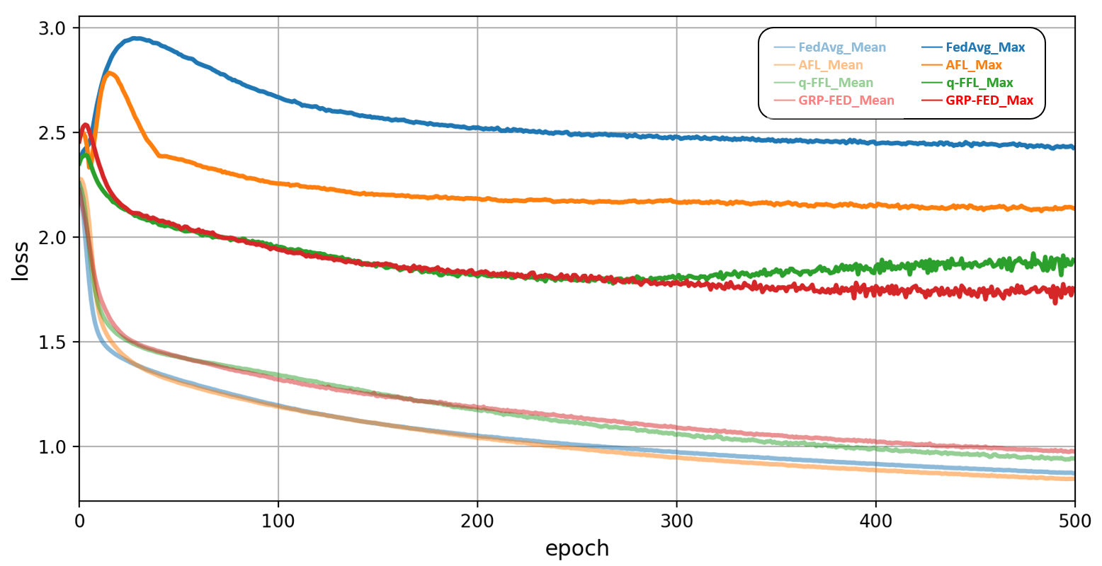
Is the Global Model Actually Fair?  To ensure the global model is actually fair, we plot the learning curve of the mean and max global training loss in Fig. 3. Basically, all methods have a relatively low mean training loss during the global training. We can investigate the global fairness through the max global training loss. FedAvg treats each client equally and sacrifices those minor classes, resulting in a high max global training loss in the end. The adversarial aggregation in AFL is not fair enough and still remains high max training loss. q-FFL adopts a constnat loss power $q$ to tune the amount of fairness. While, a fixed power of loss cannot satisfy all fairness situations and instead increases the max training loss at last. Our adaptive aggregation considers a dynamic $q$ that can adaptively adjust, which keeps decreasing the max training loss as the fairer global model.

Figure 3: Learning curve of the mean/max global training loss.

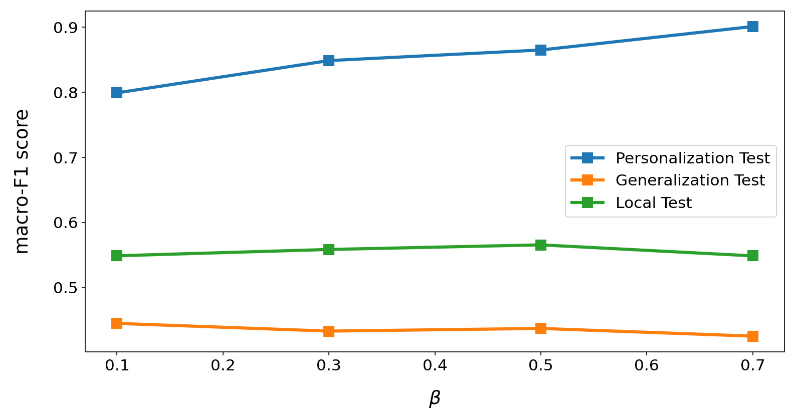
How $\beta$ affects the local models?  We adopt $\beta$ to control the weight of loss between the personalization by the local training and the generalization by the global-regularized discriminator. Fig. 4 illustrates the effect of $\beta$ on MIT-BIH during the local personalization. There is a trade-off between local personalization ($T_{p}$) and local generalization ($T_{r}$). When $\beta$ gets larger, we treat the personalization as more important and improve $T_{p}$ but hurt $T_{r}$. On the other hand, $T_{r}$ increases when $T_{p}$ decreases if we consider the local feature should be more generalized with lower $\beta$. $\beta=0.5$ leads to the best local test ($T_{l}$) in our GRP-FED.

Figure 4: The trade-off between the personalization ($T_{p}$) and generalization ($T_{r}$) in local test ($T_{l}$) under different loss weight $\beta$.

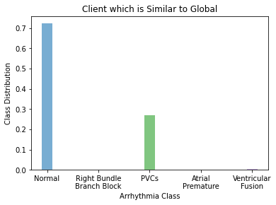
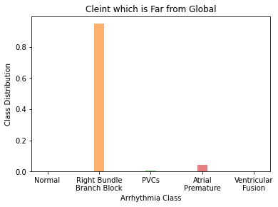
Case Study  Fig. 5 visualizes the performance of two clients on MIT-BIH. Since the upper client is similar to the global class distribution, all methods perform well under both the global test ($T_{g}$) and local personalization test ($T_{p}$). The trained local model on this client also performs well in the overall local test ($T_{l}$). However, in the lower client, which presents a distinct class distribution, LG-FedAvg is entirely overfitting and results in high $T_{p}$ but terrible $T_{l}$. By contrast, our GRP-FED still outperforms the remaining baselines in $T_{p}$ and achieves the highest $T_{l}$ with the help of the global-regularized discriminator. Moreover, GRP-FED considers the dynamic fairness from different client distributions and leads to the best $T_{g}$ as a fairer global model.

Method	Global Test	Local Test	Personalization
FedAvg	0.996	0.498	0.996
q-FFL	0.718	0.464	0.578
per-FedAvg	0.990	0.519	0.999
pFedMe	0.992	0.379	0.998
LG-FedAvg	0.999	0.380	1.000
GRP-FED	0.997	0.657	0.998

Method	Global Test	Local Test	Personalization
FedAvg	0.219	0.262	0.219
q-FFL	0.328	0.325	0.328
per-FedAvg	0.291	0.351	0.435
pFedMe	0.152	0.274	0.492
LG-FedAvg	0.269	0.178	0.975
GRP-FED	0.454	0.491	0.493

Figure 5: The performance of global test and local test in two clients (upper: similar to, lower: far from the global distribution).

5 Conclusion

In this paper, we introduce Global-Regularized Personalization (GRP-FED) to address the client imbalance issue under federated learning (FL). GRP-FED consists of a global model and local models for each client. The global model considers the dynamic fairness and investigates different proportions of clients with the adaptive aggregation. The local models do personalization by the local training, and the proposed global-regularized discriminator can prevent the overfitting issue. Extensive results show that our GRP-FED outperforms baselines under both global and local scenarios on real-world MIT-BIH and synthesis CIFAR-10 datasets.

References

- Basu et al. (2019) Basu, D., Data, D., Karakus, C., and Diggavi, S. N. Qsparse-local-sgd: Distributed SGD with quantization, sparsification and local computations. In Wallach, H. M., Larochelle, H., Beygelzimer, A., d’Alché-Buc, F., Fox, E. B., and Garnett, R. (eds.), Advances in Neural Information Processing Systems, 2019.
- Chen et al. (2020) Chen, Y., Ning, Y., Chai, Z., and Rangwala, H. Federated multi-task learning with hierarchical attention for sensor data analytics. In 2020 International Joint Conference on Neural Networks (IJCNN), 2020. doi: 10.1109/IJCNN48605.2020.9207508.
- Deng et al. (2020) Deng, Y., Kamani, M. M., and Mahdavi, M. Adaptive personalized federated learning. arXiv preprint arXiv:2003.13461, 2020.
- Dinh et al. (2020) Dinh, C. T., Tran, N. H., and Nguyen, T. D. Personalized federated learning with moreau envelopes. In Larochelle, H., Ranzato, M., Hadsell, R., Balcan, M., and Lin, H. (eds.), Advances in Neural Information Processing Systems, 2020.
- Duan et al. (2020) Duan, M., Liu, D., Chen, X., Liu, R., Tan, Y., and Liang, L. Self-balancing federated learning with global imbalanced data in mobile systems. IEEE Transactions on Parallel and Distributed Systems, 32(1):59–71, 2020.
- Fallah et al. (2020) Fallah, A., Mokhtari, A., and Ozdaglar, A. Personalized federated learning with theoretical guarantees: A model-agnostic meta-learning approach. Advances in Neural Information Processing Systems, 2020.
- Goldberger et al. (2000) Goldberger, A. L., Amaral, L. A., Glass, L., Hausdorff, J. M., Ivanov, P. C., Mark, R. G., Mietus, J. E., Moody, G. B., Peng, C.-K., and Stanley, H. E. Physiobank, physiotoolkit, and physionet: components of a new research resource for complex physiologic signals. Circulation, 101(23), 2000.
- Hanzely & Richtárik (2020) Hanzely, F. and Richtárik, P. Federated learning of a mixture of global and local models. CoRR, abs/2002.05516, 2020.
- He et al. (2016) He, K., Zhang, X., Ren, S., and Sun, J. Deep residual learning for image recognition. CVPR, 2016.
- Jiang et al. (2019) Jiang, Y., Konecný, J., Rush, K., and Kannan, S. Improving federated learning personalization via model agnostic meta learning. CoRR, abs/1909.12488, 2019.
- Kairouz et al. (2019) Kairouz, P., McMahan, H. B., Avent, B., Bellet, A., Bennis, M., Bhagoji, A. N., Bonawitz, K., Charles, Z., Cormode, G., Cummings, R., et al. Advances and open problems in federated learning. arXiv preprint arXiv:1912.04977, 2019.
- Khodak et al. (2019) Khodak, M., Balcan, M., and Talwalkar, A. S. Adaptive gradient-based meta-learning methods. In Wallach, H. M., Larochelle, H., Beygelzimer, A., d’Alché-Buc, F., Fox, E. B., and Garnett, R. (eds.), Advances in Neural Information Processing Systems, 2019.
- Konečnỳ et al. (2016) Konečnỳ, J., McMahan, H. B., Yu, F. X., Richtárik, P., Suresh, A. T., and Bacon, D. Federated learning: Strategies for improving communication efficiency. arXiv preprint arXiv:1610.05492, 2016.
- Krizhevsky & Hinton (2009) Krizhevsky, A. and Hinton, G. Learning multiple layers of features from tiny images. Master’s thesis, Department of Computer Science, University of Toronto, 2009.
- Li et al. (2019) Li, T., Sanjabi, M., Beirami, A., and Smith, V. Fair resource allocation in federated learning. arXiv preprint arXiv:1905.10497, 2019.
- Li et al. (2020) Li, Z., Kovalev, D., Qian, X., and Richtárik, P. Acceleration for compressed gradient descent in distributed and federated optimization. In Proceedings of the 37th International Conference on Machine Learning, ICML, 2020.
- Liang et al. (2020) Liang, P. P., Liu, T., Ziyin, L., Salakhutdinov, R., and Morency, L.-P. Think locally, act globally: Federated learning with local and global representations. arXiv preprint arXiv:2001.01523, 2020.
- Maaten & Hinton (2008) Maaten, L. v. d. and Hinton, G. Visualizing data using t-sne. Journal of machine learning research, 9(Nov), 2008.
- McMahan et al. (2017) McMahan, B., Moore, E., Ramage, D., Hampson, S., and y Arcas, B. A. Communication-efficient learning of deep networks from decentralized data. In Singh, A. and Zhu, X. J. (eds.), Proceedings of the 20th International Conference on Artificial Intelligence and Statistics, AISTATS, 2017.
- Mohri et al. (2019) Mohri, M., Sivek, G., and Suresh, A. T. Agnostic federated learning. In Chaudhuri, K. and Salakhutdinov, R. (eds.), Proceedings of the 36th International Conference on Machine Learning, ICML, 2019.
- Smith et al. (2017) Smith, V., Chiang, C.-K., Sanjabi, M., and Talwalkar, A. S. Federated multi-task learning. In Advances in neural information processing systems, 2017.
- Wang et al. (2021) Wang, L., Xu, S., Wang, X., and Zhu, Q. Addressing class imbalance in federated learning. In Proceedings of the AAAI Conference on Artificial Intelligence, volume 35, pp. 10165–10173, 2021.
- Yang & Xu (2020) Yang, Y. and Xu, Z. Rethinking the value of labels for improving class-imbalanced learning. In Larochelle, H., Ranzato, M., Hadsell, R., Balcan, M., and Lin, H. (eds.), Advances in Neural Information Processing Systems, 2020.