Structure of ultra-magnetised neutron stars

Abstract

In this review we discuss self-consistent methods to calculate the global structure of strongly magnetised neutron stars within the general-relativistic framework. We outline why solutions in spherical symmetry cannot be applied to strongly magnetised compact stars, and elaborate on a consistent formalism to compute rotating magnetised neutron star models. We also discuss an application of the above full numerical solution for studying the influence of strong magnetic fields on the radius and crust thickness of magnetars. The above technique is also applied to construct a “universal” magnetic field profile inside the neutron star, that may be useful for studies in nuclear physics. The methodology developed here is particularly useful to interpret multi-messenger astrophysical data of strongly magnetised neutron stars.

1 Introduction

The phase diagram of Quantum Chromodynamics (QCD), that describes the behaviour of matter at different densities and temperatures, has intrigued physicists since decades. While low density and low temperature physics is probed in terrestrial nuclear experiments, finite temperatures and densities are accessible to heavy-ion collision experiments. High temperature and low density physics is of relevance to the early Universe and can be probed with techniques such a Lattice QCD. Neutron stars (NS), on the other hand, allow us to investigate the high density low temperature regime of the phase diagram that is complementary to terrestrial experiments. Hot proto-neutron stars newly born from core collapse supernovae or binary neutron star mergers lie in the finite temperature part of the phase diagram. The understanding of the nature of dense matter encompasses many different disciplines in physics. Comparison of information from the different regimes of the phase diagram provides important input in understanding the behaviour of dense matter under extreme conditions.

Another important question in this regard is the nature of the QCD phase diagram under strong magnetic fields. An important insight can come from observations of neutron stars (pulsars) endowed with strong magnetic fields. In general, standard pulsars are known to have large surface magnetic fields around $10^{10}-10^{12}$ G. This can be explained by the conservation of flux of the progenitor star as it collapses to a neutron star via a core-collapse supernova explosion. Further, astrophysical observations indicate the existence of a class of neutron stars possessing ultra-strong magnetic fields, commonly referred to as magnetars (see e.g. the pioneering articles Duncan92 ; Usov92 ; Paczynski and the review Kaspi for a comprehensive understanding). It is commonly thought that magnetars are observed as Anomalous X-ray Pulsars (AXPs) and Short Gamma-ray Repeaters (SGRs). From the characteristic common features such as eruptive emission of X-rays and gamma rays, it has been concluded that the energy associated with these bursts of intense radiation CotiZelati is probably due to ultra-strong magnetic fields, with surface fields reaching $10^{15}-10^{16}$ G. Recently, isolated neutron stars, such as X-ray Dim Isolated NSs (XDINSs) and Rotating Radio Transients (RRATs) with intermediate magnetic field strengths have also been observed Popov . Multi-messenger observations of the compact remnant resulting from the neutron star merger event GW170817 also suggest that it may be a hypermassive differentially rotating magnetar Tong ; Ai ; Gill . Similarly, the observation of GRB 200522A was associated with the formation of a stable magnetar, in order to explain some of the afterglow emission Fong . Thus for the correct interpretation of astrophysical data from strongly magnetised neutron stars, it is crucial to develop accurate models of the structure of such objects.

This article is organised as follows: in Sec. 2 we briefly recall the maximal value of the magnetic field inside compact stars, before discussing in Sec. 3 its effects on star’s microscopic and macroscopic properties. Sec. 4 describes the numerical approach to get numerical models of strongly magnetised compact stars, which is then applied in Sec. 5 to compute the effect of a magnetised equation of state on their structure. In Sec. 6 we devise a so-called universal profile for magnetic field distribution in compact stars, before giving in Sec. 7 some concluding remarks. Unless otherwise stated (in particular when discussing magnetic field values) we use natural (Dirac) units such that $G=c=\hbar=1$.

2 Maximum interior magnetic field

Several observations can be used to estimate the surface magnetic fields in magnetars. From the measurements of pulsar rotation periods and period derivatives (so-called $P-\dot{P}$ diagram), assuming a dipole model for the magnetic field, one can estimate the magnetic fields to be $\sim 10^{15}-10^{16}$ G for some objects. Direct estimates of the field on the surface of magnetars is also possible through the observation of cyclotron lines Ibrahim ; Mereghetti .

However, there are no astrophysical observations to directly measure the magnetic field at the centre of a neutron star. Applying the Virial Theorem (comparison of magnetic energy with that of matter and gravitational potential energy) ChandraFermi ; Shapiro ; Bonazzola94 ; Gourgoulhon94 , the estimate of the maximum magnetic field strength in the interior of a magnetar turns out to be $\sim 10^{18}$ G. However, the exact estimate of the maximum central field in this way is also complicated, as these energy contributions in turn also depend on magnetic field.

3 Effects of strong magnetic field

Ultrastrong interior magnetic field strengths $\sim 10^{18}$ G may affect compact stars mainly in two ways:

• The magnetic field interacts with the particles in the stellar interior, thus affecting the Equation of State (EoS)

• Strong magnetic fields result in a modification of the energy-momentum tensor, breaking of the spherical symmetry, and therefore affect the external structure of the compact star.

We elaborate on these aspects in detail in the following sections.

3.1 Effect on the Equation of state

Since for neutron stars older than several minutes the typical temperatures are negligible for the equation of state, we will consider here only the $T=0$ case. In addition we assume matter to be in chemical ($\beta$) equilibrium. In the NS interior, charge conservation and chemical equilibrium result in the appearance of a small fraction of protons and electrons, in addition to neutrons. Further, as the baryon densities in the NS interior surpass $\sim$ 2-3 times that of nuclear saturation density ($n_{0}\sim 2.3\times 10^{17}$ kg/m³), strangeness containing particles such as hyperons, condensates of kaons or even deconfined quarks may appear there (see Ref. Haensel2007 for detailed discussions). The appearance of these particles depends on an interplay between the neutron and electron chemical potentials that govern the weak interactions that produce them. The composition of the NS core affects the relation between the matter pressure and energy density (EoS), see e.g. ChatterjeeVidana .

In presence of a magnetic field, the motion of charged particles becomes confined to quantised Landau levels Landau and on one hand the EoS is affected by the Landau quantisation of the charged particles (such as protons, electrons, etc). The effects are most pronounced when the particle is confined to the lowest Landau level. Additionally, as first studied by Canuto and Chiu Canuto in the case of a relativistic electron gas, the energy-momentum tensor becomes anisotropic. On the other hand, the interaction of the magnetic moments, including the anomalous magnetic moments of the neutral particles (such as neutrons, $\Lambda$-hyperons, …), with the magnetic field influences the EoS.

The effect of quantising magnetic fields on the EoS for different models of NS matter can be found in many articles in the literature, see e.g. Bandyopadhyay ; Chakrabarty ; Broderick00 ; Broderick02 ; Strickland ; Noronha ; Rabhi ; Ferrer ; Sinha . In presence of a uniform external magnetic field in the $z$ direction, the transverse momenta of particles (electrons, protons, hyperons) are restricted to discrete Landau levels with squared transverse momenta $k_{\perp}^{2}=2\nu qb$ where $\nu\geq 0$ is the Landau quantum number. For spin-1/2 particles, $\nu$ is related to the orbital angular momentum $n$ by

$$\nu=n+\frac{1}{2}-\frac{s}{2}\frac{q}{\lvert{q}\rvert}~{},$$ (1)

where $s\pm 1$ is the spin projection of the particle in the direction of the magnetic field. The total energy of a charged particle becomes quantised as (see Broderick00 ):

$$E=\sqrt{k_{z}^{2}+\left[(m^{2}+2\nu\lvert{q}\rvert b)^{1/2}-s\kappa b\right]^{2}}=\sqrt{k_{z}^{2}+\bar{m}^{2}(\nu)}~{},$$ (2)

$k_{z}$ being the momenta in the $z$-direction and $\kappa$ the anomalous magnetic moment Strickland , while

$$\bar{m}^{2}(\nu)=(\sqrt{m^{2}+2\nu\lvert q\rvert b}-s\kappa b)^{2}~{}.$$ (3)

If one considers the simplest case with $\kappa=0$, the maximum momentum $k_{z}$ in terms of the chemical potential $\mu$ is defined as:

$$k_{z,F}=\sqrt{\mu^{2}-2\nu\lvert q\rvert b-m^{2}}~{}.$$ (4)

To ensure that the quantity under the square root is positive, one may impose the condition:

$$\nu\leq\nu_{max}=\left[\frac{\mu^{2}-m^{2}}{2\lvert q\rvert b}\right]~{}.$$ (5)

A magnetic field strong enough such that only the lowest Landau level is occupied is in general called a strongly quantising field. Using the above relations, one can write down the expression for the number density as

$$n=\frac{\lvert q\rvert b}{2\pi^{2}}\sum_{s=\pm 1}\sum_{\nu=0}^{\nu_{max}}k_{z,F}(\nu)~{}.$$ (6)

Similarly, one can obtain the energy density as

$$\epsilon=\frac{\lvert q\rvert b}{2\pi^{2}}\sum_{s=\pm 1}\sum_{\nu=0}^{\nu_{max}}\int_{0}^{k_{z,F}}dk_{z}\sqrt{k_{z}^{2}+\bar{m}^{2}(\nu)}~{}.$$ (7)

From the energy density, one may derive the pressure using the Gibbs-Duhem relation, and therefore obtain the EoS. The situation is more complicated in the presence of non-zero anomalous magnetic moment Strickland , and the full expression in Eq. (2) has to be used.

As mentioned above, these effects have been included in numerous studies of the neutron star matter EoS in a strong magnetic field. In the neutron star crust, due to the magnetic field electronic motion is quantised into Landau levels. For field strengths $b\gg b^{e}_{c}$, the crust composition depends on the magnetic field strength with typical quantum oscillations observed in the transition density from one nuclear cluster to another. $b^{e}_{c}=m_{e}^{2}/|e|\sim 4.4\times 10^{13}$ G denotes here the critical field for electrons Haensel2007 . If the magnetic field strength exceeds the value for being strongly quantising, this transition density is increasing linearly with the magnetic field strength, leading to a less neutron rich crust and an increased density for neutron drip, i.e. shifting the transition from the outer to the inner crust to higher densities Chamel2015 . In the transition region from the inner to the outer crust, field strengths above roughly $\sim 1300b^{e}_{c}$ correspond to strongly quantising fields. In the crust, for magnetic fields above a few times $10^{17}$ G, nuclear binding energies start to become significantly altered, modifying additionally the structure of the crust, see e.g. Pena . A summary of crust properties under strong magnetic fields can be found in Ref. BlaschkeChamel .

The crust-core interface is characterised by the transition from inhomogeneous matter in the crust to homogeneous matter in the core. Ravenhall et al. Ravenhall1984 and Hashimoto et al. Hashimoto1984 predicted that this transition passes via more and more deformed nuclei, forming the so-called ”nuclear pasta”, with the detailed structure depending on the nuclear interaction. Meanwhile, different calculations and numerical techniques have been used to investigate the crust-core interface region, see e.g.Oyamatsu ; Pethick ; Watanabe ; Avancini2008 ; Ducoin2010 ; Avancini2010 ; Providencia2017 , confirming essentially the above picture and obtaining comparable values for crust-core transition densities. The crust-core region of magnetars was recently studied within the relativistic mean field model framework Fang2016 ; Fang2017 . In these works, the effects of strong magnetic fields ($10^{15}-10^{17}$ G) on the instability region was investigated with the help of the Vlasov formalism used to determine the dynamical spinodals. It is found that again, since the inner crust becomes less neutron rich, the transition to homogeneous matter is shifted to higher densities, see also Paisthisissue .

For homogeneous hadronic matter, be it purely nucleonic or including additional particles such as hyperons or $\Delta$-baryons, the effect of a strong magnetic field on the EoS has been discussed for instance in Refs. Broderick00 ; Broderick02 ; Rabhi2008 ; Sinha ; Haber ; Dexheimer2021 using different models for the underlying hadronic interaction. As can be easily estimated from the value of the critical magnetic field for the different hadrons and the energy of the interaction of the respective magnetic moments with the magnetic field, below a field strength of $\sim 10^{18}$ G almost no influence on the EoS is expected. As an example we show in Fig. 1 the EoS, i.e. pressure as function of energy density for cold, $\beta$-equilibrated matter, for two different nucleonic models Rabhi2008 from the family of covariant density functional theory, DD2 DD2 and TM1 TM1 , for different magnetic field strengths. It is obvious that indeed at $b=10^{18}$ G the EoS is still almost indistinguishable from the EoS without magnetic field, whereas at $b=10^{19}$ G the impact of the magnetic field on the EoS becomes non-negligible.

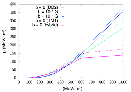
Figure 1: The effect of magnetic field on two hadronic EoS of neutron star matter Rabhi2008 , using the DD2 DD2 and the TM1 TM1 nuclear interaction, respectively, as well as the hybrid EoS discussed in Dexheimer2012 .

Since the magnetic field influences quark and hadronic matter in a different way, it has an impact on the potential transition from hadronic to quark matter, too. This question has been addressed by several authors, see e.g. Rabhi ; Dexheimer2012 . In Fig. 1 we show as an example the results from the study of Dexheimer2012 . It is based on a chiral sigma model description of both, the hadronic and the quark phase. The density for the onset of quark matter is clearly visible from the kink in the EoS. Actually, within the density range shown in the figure, only the hadronic and a mixed phase are visible, whereas the pure quark phase is present only at higher densities. In the present model, no pure quark phase is reached in the interior of neutron stars. As can be seen from the figure, a strong magnetic field pushes the onset of quark matter to higher densities and pressures, thus further delaying the appearance of a potential quark core in neutron stars. In other studies, it is found in a similar way that a strong magnetic field shifts the transition to quark matter to higher densities, see the review Menezeshere , too.

The influence of the magnetic field on quark matter has attracted much interest,among others due to the impact on the complex structure of the QCD phase diagram and phenomena such as magnetic catalysis, see e.g. Schmitt for a review, and several authors have considered quark matter in compact stars with a strong magnetic field, see e.g. Bandyopadhyay ; Noronha ; Gatto ; Ferrer2013 ; Ferrer2020 and references therein. Two examples for influence of a strong magnetic field on the EoS of quark matter in a compact star are shown in Fig. 2. The first one Avancini uses the Nambu- Jona-Lasinio (NJL) model without pairing interaction, whereas for the second one a simple massless three-flavor MIT bag model was applied, including a pairing interaction of NJL-type to account for the possibility of colour superconductivity in the so-called magnetic colour-flavor locked state (mCFL) Chatterjee2015 , see also Noronha . The most favored phase of QCD at high densities is the colour-flavor-locked (CFL) superconducting phase and, for a magnetic field strength of the order of the quark energy gap, such a mCFL phase is preferred.

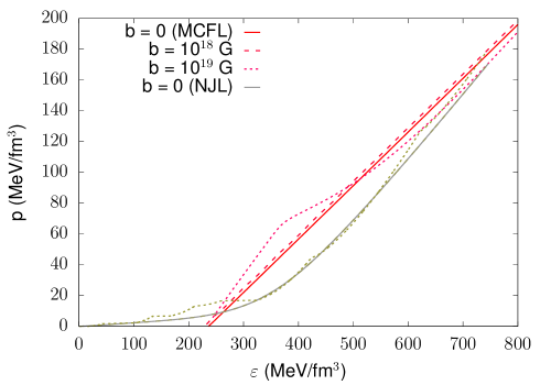
Figure 2: The effect of magnetic field on the quark matter EoS in the NJL model discussed in Avancini and the mCFL model discussed in Chatterjee2015 .

Again, the effect of magnetic fields starts to become evident only for very large fields above 10¹⁸ G. For $b=10^{19}$ G in both models the de Haas van Alphen oscillations due to the Landau quantisation of charged particles are clearly visible. The dimensionless ratio $x$ of magnetisation to the magnetic field, see Eq. (14) below, is shown in Fig.  3 for the mCFL model for two values of baryon number chemical potential. Here again, the de Haas van Alphen oscillations are clearly visible and become more and more pronounced with increasing magnetic field strengths as expected, see also the discussion in Noronha .

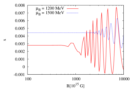
Figure 3: Dimensionless ratio $x$, see Eq. (14), of magnetisation to the magnetic field as a function of magnetic field strength $b$ in the mCFL phase showing the de Haas van Alphen oscillations Chatterjee2015 .

3.2 Effects on external structure

Stellar structure is determined in General Relativity by equations describing the stationary configuration for the fluid, and the Einstein field equations. The energy- momentum tensor, containing matter properties of the star, enters the stellar structure equations as the source of the Einstein equations. Neglecting the coupling to the electromagnetic field, one generally assumes a perfect fluid and the energy-momentum tensor takes the following form

$$T_{f}^{\mu\nu}=(\varepsilon+p)\;u^{\mu}u^{\nu}+p\;g^{\mu\nu}~{},$$ (8)

where $\varepsilon$ denotes the (matter) energy density, $p$ the pressure, and $u^{\mu}$ the fluid four-velocity. The EoS then relates pressure and energy density to the relevant thermodynamic quantities. In  Chatterjee2015 , the general expression for the energy-momentum tensor in presence of an electromagnetic field was derived, starting with a microscopic Lagrangian including interaction between matter (fermions denoted by $\psi$) and the electromagnetic field $F_{\mu\nu}$

$${\cal L}=-\bar{\psi}(x)(D_{\mu}\gamma^{\mu}+m)\psi(x)-\frac{1}{4\mu_{0}}F_{\mu\nu}F^{\mu\nu}~{},$$ (9)

where $D_{\mu}=\partial_{\mu}-iqA_{\mu}$ with the charge $q$ of the particle. $\mu_{0}$ is the vacuum permeability. $F^{\mu\nu}$ is the field strength tensor of the electromagnetic field

$$F^{\mu\nu}=\partial^{\mu}A^{\nu}-\partial^{\nu}A^{\mu}~{},$$ (10)

It was demonstrated that the thermal average of the energy-momentum tensor is given by  Chatterjee2015

$$\langle T^{\mu\nu}\rangle = (\varepsilon+p)\;u^{\mu}u^{\nu}+p\;g^{\mu\nu}$$ (11)

$$+\frac{1}{2}(F^{\nu}_{\;\tau}M^{\tau\mu}+F^{\mu}_{\;\tau}M^{\tau\nu})$$

$$-\frac{1}{\mu_{0}}(F^{\mu\alpha}F_{\alpha}^{\,\nu}+\frac{g^{\mu\nu}}{4}F_{\alpha\beta}F^{\alpha\beta})~{}.$$

The first two terms on the right hand side of Eq. (11) are the perfect fluid fermionic contribution, followed by the magnetisation term and finally the electromagnetic field contributions to the energy-momentum tensor.

According to Ohm’s Law, and assuming that the matter has an infinite conductivity, the electric field as measured by the fluid comoving observer must be zero, and in the fluid rest frame (FRF) only the magnetic field $b_{\mu}$ is nonzero. The electromagnetic field tensor can then be expressed as Gourgoulhon

$$F_{\mu\nu}=\epsilon_{\alpha\beta\mu\nu}u^{\beta}b^{\alpha}~{}.$$ (12)

Assuming an isotropic medium and a magnetisation parallel to the magnetic field, the magnetisation tensor $M_{\mu\nu}$ can be written as

$$M_{\mu\nu}=\epsilon_{\alpha\beta\mu\nu}u^{\beta}a^{\alpha}~{},$$ (13)

where the magnetization four-vector is defined as

$$a_{\mu}=\frac{x}{\mu_{0}}b_{\mu}$$ (14)

Employing Eqs. (12,13), the energy-momentum tensor can be rewritten in the following way

$$T^{\mu\nu} = T_{f}^{\mu\nu}+\frac{1}{\mu_{0}}\left(-b^{\mu}b^{\nu}+(b\cdot b)u^{\mu}u^{\nu}+\frac{1}{2}g^{\mu\nu}(b\cdot b)\right)$$ (15)

$$+\frac{x}{\mu_{0}}\left(b^{\mu}b^{\nu}-(b\cdot b)(u^{\mu}u^{\nu}+g^{\mu\nu})\right)~{}.$$

In the absence of magnetisation, i.e. for $x=0$, this expression reduces to the standard MHD form for the energy-momentum tensor Gourgoulhon .

It is important here to point out that the magnetic field does not induce an anisotropy in the thermodynamic matter pressure, obtained from the derivative of the partition function. Rather magnetic fields result in an anisotropy of the energy momentum tensor and break spherical symmetry. Consequently with increasing strength of the magnetic field, the shape of a magnetar departs more and more from a spherical shape, to that of an oblate or prolate spheroid, depending on the configuration of the field. If the spatial elements of the FRF energy-momentum tensor are interpreted as pressures, then there is a difference induced by the orientation of the magnetic field, often tabbed “parallel” and “perpendicular” pressures in the literature. To be precise, let us consider a magnetic field pointing in $z$-direction. The energy-momentum tensor can then be decomposed into the sum of matter and field contributions $T_{\mu\nu}=T^{\mu\nu}_{m}+T^{\mu\nu}_{B}$ as follows:

$$T^{\mu\nu}_{m}=\begin{pmatrix}\varepsilon&0&0&0\\ 0&p-ab&0&0\\ 0&0&p-ab&0\\ 0&0&0&p\end{pmatrix}$$ (16)

where the first term is related to the fluid energy density and the other three non-zero terms are associated with the matter pressure in $x,y,z$ coordinates, $a$ being the magnetisation. Similarly, the electromagnetic contribution to the energy momentum tensor in the FRF becomes:

$$T^{\mu\nu}_{B}=\frac{1}{\mu_{0}}\begin{pmatrix}\frac{1}{2}b^{2}&0&0&0\\ 0&\frac{1}{2}b^{2}&0&0\\ 0&0&\frac{1}{2}b^{2}&0\\ 0&0&0&-\frac{1}{2}b^{2}~{}.\end{pmatrix}$$ (17)

The spatial elements $T^{11}=T^{22}$ are then interpreted as perpendicular pressure ($p_{\perp}=p-ab+b^{2}/2$) and the element $T^{33}$ as parallel one ($p_{\parallel}=p-b^{2}/2$) Ferrer ; Paulucci ; Dexheimer2014 . It should, however, be kept in mind that these do not correspond to the thermodynamic pressure, and have a meaning only as elements of the energy-momentum tensor $T^{\mu\nu}$.

It should be stressed in addition, see the argumentation in Blandford and Potekhin , that upon computing equilibrium, the magnetisation contribution to the energy-momentum tensor is cancelled by the Lorentz force associated with magnetisation. Thus, although the magnetic field induces an anisotropy in the matter part of the energy-momentum tensor, only the isotropic thermodynamic pressure $p$ is relevant for determining equilibrium. This conjecture Blandford has been confirmed by the derivation of the magnetostatic equilibrium equations in Chatterjee2015 , see the discussion in Sec. 4.2 below.

3.2.1 TOV equations

For spherically symmetric neutron stars in static equilibrium, given an EoS, the global structure (e.g. mass, radius) can be calculated using the well known Tolman Oppenheimer Volkoff (TOV) equations of hydrostatic equilibrium:

$$\frac{d\ell}{dr} = 4\pi r^{2}\varepsilon(r)~{},$$

$$\frac{d\nu}{dr} = \left(\ell(r)+4\pi r^{3}p(r)\right)\frac{1}{r^{2}}\left(1-\frac{2\ell}{r}\right)^{-1}~{},$$

$$\frac{dp}{dr} = -\left(\varepsilon(r)+p(r)\right)\frac{d\nu}{dr}~{}.$$ (18)

Here $\ell(r)$ and $\nu(r)$ are gravitational potentials for the line element in spherical coordinates:

$$ds^{2}=-e^{2\nu(r)}dt^{2}+\left(1-\frac{2\ell}{r}\right)^{-1}dr^{2}+r^{2}(d\theta^{2}+\sin^{2}\theta d\phi^{2})~{}.$$ (19)

The pressure and energy density profiles $p(r)$ and $\varepsilon(r)$ are related through the EoS.

The question arises whether spherical TOV equations can be applied to describe magnetar structure, given that magnetars are highly deformed from their spherical shape and that a magnetic field cannot be described in spherical symmetry, as there are no magnetic monopoles. There exist several works in the literature that attempted to compute the mass-radius relations of strongly magnetised NSs as a first approach using isotropic TOV equations Strickland ; Rabhi ; Ferrer ; Paulucci ; Lopes ; Dexheimer2014 ; Casali . In such works, the different components of the macroscopic energy-momentum tensor in the FRF are used to obtain the energy density $\varepsilon$, parallel, $p_{\parallel}$, and perpendicular, $p_{\perp}$, pressures, respectively. However, this procedure necessarily induces confusion, since the TOV equations only admit one pressure.

The impossibility to apply spherically symmetric TOV equations in presence of a magnetic fields can also be understood by inspecting the most general solution of the equations of hydrostatic equilibrium in general relativity for the spherically symmetric case. The coupled system of structure equations was derived by Bowers and Liang  Bowers

$$\frac{d\ell}{d\bar{r}} = 4\pi\bar{r}^{2}\varepsilon$$

$$\frac{d\nu}{d\bar{r}} = \left(\ell+4\pi\bar{r}^{3}p_{r}\right)\frac{1}{\bar{r}^{2}}\left(1-\frac{2\ell}{\bar{r}}\right)^{-1}$$

$$\frac{dp_{r}}{d\bar{r}} = -\left(\varepsilon+p_{r}\right)\frac{d\nu}{d\bar{r}}+\frac{2}{\bar{r}}(p_{\perp}-p_{r})~{},$$ (20)

with the most general energy-momentum tensor compatible with spherical symmetry given by

$$T^{\mu\nu}=\mathrm{diag}(\varepsilon,p_{r},p_{\perp},p_{\perp})~{},$$ (21)

where $p_{r}$ and $p_{\perp}$ are the radial and tangential pressure components. In the perfect-fluid model (8) $p_{r}=p_{\perp}$, and it might be tempting to cast an energy-momentum tensor for a magnetic field pointing in $z$-direction into this form, assuming a perfect conductor and isotropic matter. However, in the case of the electromagnetic energy-momentum tensor $T^{\theta\theta}\neq T^{\phi\phi}$ (see e.g. Eqs. (23d)-(23e) of Chatterjee2015 ), in clear contradiction with the assumption of Bowers and Liang (21) in spherical symmetry. Further, $\lim_{r\to 0}(T^{rr}-T^{\theta\theta})\not=0$ and thus, the last term in Eq. (20) diverges at the origin. This discussion shows that there cannot be any correct description of the magnetic field in spherical symmetry.

3.2.2 Perturbative approach

For low magnetic fields, Konno et al. Konno obtained an analytical solution for the external structure using a perturbative approach. There have been also attempts Mallick to compute the structure of neutron stars in strong magnetic fields by a simple Taylor expansion of the energy-momentum tensor and the metric around the spherically symmetric case, but these deviations are significant at ultrastrong magnetic fields relevant for magnetars. Such solutions are not applicable in the presence of large quantising magnetic fields.

3.2.3 Numerical solutions with non-magnetised EoSs

Bocquet et al. Bocquet were the first to include magnetic fields to rotating neutron star models, by solving coupled Einstein-Maxwell equations. Subsequently several groups performed fully relativistic numerical computations of the magnetar structure by taking into account the anisotropy of the stress-energy tensor Cardall ; Kiuchi2008 ; Oron ; Ioka ; KiuchiKotake ; Yasutake ; Yoshida ; Bucciantini . However, such studies assume a perfect fluid, polytrope or a realistic EoS, but do not take into account the magnetic field modifications due the quantising magnetic field, described in Sec. 3.1.

The internal composition, particularly the nuclear EoS, affects the macroscopic structure as well as observable properties of neutron stars, such as cooling and emission of gravitational waves. Correct interpretation of astrophysical data, in the era of multi-messenger astronomy, calls for the need to develop consistent numerical models of magnetars, taking into account the effect of strong magnetic fields both on the microphysics and macrophysics. Ideally, one must solve the coupled Einstein-Maxwell equations, along with a magnetic field dependent EoS, to obtain the global quantities. This is described in Sec. 4.

4 Numerical Models of strongly magnetised compact stars

In the preceding sections Sec. 3.1 and Sec. 3.2, we discussed how ultrastrong magnetic fields affect the internal and external structure of magnetars. In this section, we describe how global numerical models for the same, within the framework of general relativity, can be obtained in a consistent way.

Within the framework of general relativity, we follow BGSM to make the assumption of a stationary, axisymmetric spacetime, in which the matter part (the energy-momentum tensor) fulfills the circularity condition. The line element in these coordinates can be written as :

$${\rm d}s^{2} = -N^{2}\,{\rm d}t^{2}+B^{2}r^{2}\sin^{2}\theta\left({\rm d}\varphi-N^{\varphi}\,{\rm d}t\right)^{2}$$ (22)

$$+A^{2}\left({\rm d}r^{2}+r^{2}\,{\rm d}\theta^{2}\right),$$

where the gravitational potentials $N,N^{\varphi},A$ and $B$ are functions of coordinates $(r,\theta)$. An important point of full general-relativistic models is that the magnetic field enters the sources of the gravitational field equations (Einstein equations). However, the main influence of magnetic field is in the equilibrium balance, with a contribution of a Lorentz-like force (see Sec. 4.2).

4.1 Maxwell equations

The electromagnetic field is assumed here to originate from free currents $j^{\sigma}$ Bocquet ; Chatterjee2015 , a priori independent from the movements of inert mass (with 4-velocity $u^{\mu}$). This assumption is a limitation of the model, and in principle one should derive a distribution for the free currents using a multifluid approach to model the movements of free charged particles, but this is beyond the scope of this article. The four-potential $A_{\mu}$ that enters in the definition of the electromagnetic field tensor $F^{\mu\nu}$ through Eq. (10), can generate simple configurations of either purely poloidal or a purely toroidal magnetic field Kiuchi2008 ; Frieben . It has been suggested via analytical considerations Tayler ; Markey and later confirmed via numerical simulations, see e.g. Braithwaite2006 ; Braithwaite2007 , that such configurations are unstable. The instability can rapidly rearrange the magnetic configuration of the stars into a mixed configuration of poloidal and toroidal fields. Solutions in mixed toroidal-poloidal configurations have been developed in the Conformally Flat Condition Bucciantini and recently, a new code (COCAL) has been obtained for such mixed toroidal-poloidal configurations in the general axisymmetric (and non-circular) spacetimes Uryu . However in this article, we confine our discussion to a simple configuration, a purely poloidal one. In this context it should be mentioned that the toroidal component is expected to assume higher field strengths than the poloidal one Akgun . However, the maximum values estimated from the observed surface fields and the virial theorem, see Sec. 2, should not be exceeded in realistic situations, such that the poloidal configuration with field strengths of $10^{18}$ G and above should already give a fairly good idea about magnetic field effects on the EoS and stellar structure.

For a purely poloidal configuration, i.e., the four-potential has vanishing components $A_{r}=A_{\theta}=0$. The electric and magnetic fields as seen by the Eulerian observer (whose four-velocity is $n^{\mu}$) are then defined as $E_{\mu}=F_{\mu\nu}\,n^{\nu}$ and $B_{\mu}=-\frac{1}{2}\epsilon_{\mu\nu\alpha\beta}\,n^{\nu}\,F^{\alpha\beta}$, with $\epsilon_{\mu\nu\alpha\beta}$ the Levi-Civita tensor associated with the metric (22). Then the non-zero components of the magnetic field are:

$$B_{r} = \frac{1}{Br^{2}\sin\theta}\frac{\partial{A_{\varphi}}}{\partial{\theta}}$$ (23a)

$$B_{\theta} = -\frac{1}{B\sin\theta}\frac{\partial{A_{\varphi}}}{\partial{r}}$$ (23b)

The homogeneous Maxwell (Faraday-Gauss) equation $F_{[\mu\nu;\lambda]}=0$ is automatically fulfilled, for the $F^{\mu\nu}$ tensor form in Eq. (10). The inhomogeneous Maxwell (Gauss-Ampère) equation in presence of external magnetic field is the covariant derivative associated with the metric (given in Eq. 22)),

$$\frac{1}{\mu_{0}}\nabla_{\mu}F^{\nu\mu}=j_{\ \mathit{free}}^{\nu}+\nabla_{\mu}M^{\nu\mu}~{},$$ (24)

can then be transformed to give

$$\nabla_{\mu}F^{\sigma\mu}=\frac{1}{1-x}(\mu_{0}j_{\ \mathit{free}}^{\sigma}+F^{\sigma\mu}\nabla_{\mu}x)~{}.$$ (25)

This equation can be expressed in terms of the two non-vanishing components of $A^{\mu}$, with the Maxwell-Gauss and the Maxwell-Ampère equations taking the form of Poisson-like partial-derivative equations (see Chatterjee2015 for details).

4.2 Equilibrium equations

The stellar equilibrium is defined by the conditions of conservation of energy and momentum. The equations can be derived from the vanishing divergence of the energy-momentum tensor:

$$\nabla_{\mu}T^{\mu\nu}=0.$$ (26)

From the expression of the energy-momentum tensor (Eq.  11), the equilibrium equation in the presence of electromagnetic field is:

$$\nabla_{\alpha}T^{\alpha\beta}=\nabla_{\alpha}T_{f}^{\alpha\beta}-F^{\beta\nu}j^{\mathit{\ }free}_{\nu}-\frac{x}{2\mu_{0}}F_{\sigma\tau}\nabla^{\beta}F^{\sigma\tau}~{},$$ (27)

where $T_{f}^{\alpha\beta}$ represents the perfect-fluid contribution to the energy-momentum tensor (8) while the second term denotes the usual Lorentz force term, arising from free currents.

In the case of rigid rotation (constant $\Omega$), a first integral of the following expression is required Bocquet

$$(\varepsilon+p)\left(\frac{1}{\varepsilon+p}\frac{\partial p}{\partial x^{i}}+\frac{1}{N}\frac{\partial N}{\partial x^{i}}-\frac{\partial\ln\Gamma}{\partial x^{i}}\right)-F_{i\rho}j^{\rho}_{\ \mathit{free}}=0~{},$$ (28)

where $N$ is the lapse function from the metric defined in Eq. (22) and $\Gamma$ the fluid Lorentz factor. Each term can be interpreted physically: pressure gradient, gravitational force, centrifugal force and Lorentz force.

In order to calculate this first integral, one introduces the enthalpy per baryon and its derivatives. It can be shown that, even in the presence of the magnetic field, the logarithm of the enthalpy per baryon represents again a first integral of the fluid equations. Note that for the neutron star case with a magnetic field in beta-equilibrium and at zero temperature, the enthalpy is a function of both baryon density and magnetic field (with $b^{2}=b_{\mu}b^{\mu}$):

$$h=h(n_{b},b)=\frac{\varepsilon+p}{n_{b}}=\mu_{b}~{}.$$ (29)

Hence one gets

$$\frac{\partial\ln h}{\partial x^{i}}=\frac{1}{h}\left(\left.\frac{\partial h}{\partial n_{b}}\right|_{b}\frac{\partial n_{b}}{\partial x^{i}}+\left.\frac{\partial h}{\partial b}\right|_{n_{b}}\frac{\partial b}{\partial x^{i}}\right)~{}.$$ (30)

In addition, the following thermodynamic relations are valid under the present assumptions

$$\left.\frac{\partial h}{\partial n_{b}}\right|_{b} = \frac{1}{n_{b}}\frac{\partial p}{\partial n_{b}}$$ (31)

$$\left.\frac{\partial p}{\partial b}\right|_{\mu_{b}} = a(=\sqrt{a^{\mu}a_{\mu}})=-\left.\frac{\partial\varepsilon}{\partial b}\right|_{n_{b}}~{}.$$ (32)

And one obtains for the derivative of the logarithm of the enthalpy

$$\frac{\partial\ln h}{\partial x^{i}} = \frac{1}{\varepsilon+p}\left[\left.\frac{\partial p}{\partial n_{b}}\right|_{b}\frac{\partial n_{b}}{\partial x^{i}}+\left(\left.\frac{\partial p}{\partial b}\right|_{n_{b}}-a\right)\frac{\partial b}{\partial x^{i}}\right]$$ (33)

$$= \frac{1}{\varepsilon+p}\left(\frac{\partial p}{\partial x^{i}}-a\frac{\partial b}{\partial x^{i}}\right)~{}.$$

Assuming that matter is a perfect conductor ($A_{t}=-\Omega A_{\varphi}$ inside the star), it is possible to relate the components of the electric current to the electromagnetic potential $A_{\varphi}$, through an arbitrary function $f$, called the current function:

$$j^{\varphi}-\Omega j^{t}=(\varepsilon+p)f\left(A_{\varphi}\right).$$ (34)

Under these assumptions, the Lorentz force term becomes

$$F_{i\rho}j^{\rho}_{\ \mathit{free}}=\left(j^{\varphi}-\Omega j^{t}\right)\frac{\partial{A_{\varphi}}}{\partial{x^{i}}}=-\left(\varepsilon+p\right)\frac{\partial{\Pi}}{\partial{x^{i}}},$$ (35)

with

$$\Pi(r,\theta)=-\int_{0}^{A_{\varphi}(r,\theta)}f(x){\rm d}x.$$ (36)

The last term can be written in terms of the magnetic field $b^{\mu}$ as:

$$\frac{x}{2\mu_{0}}F_{\mu\nu}\nabla_{i}F^{\mu\nu}=\frac{x}{\mu_{0}}\left(b_{\mu}\nabla_{i}b^{\mu}-b_{\mu}b^{\mu}u_{\nu}\nabla_{i}u^{\nu}\right)=a\frac{\partial{b}}{\partial{x^{i}}},$$ (37)

from the expression (12). Thus, this last term cancels with its counterpart in Eq. (33) and the first integral (28) keeps exactly the same form as without magnetisation:

$$\ln h(r,\theta)+\nu(r,\theta)-\ln\Gamma(r,\theta)+\Pi(r,\theta)={\rm const}.$$ (38)

4.3 Numerical resolution

As discussed in Sec. 4.1, the methodology discussed in this article is valid for the chosen poloidal geometry but other configurations such as purely toroidal or mixed ones have also been discussed elsewhere Kiuchi2008 ; Frieben ; KiuchiKotake ; Yasutake ; Bucciantini , but without taking into the magnetic field dependence of the EoS and magnetisation. The Einstein-Maxwell equations can be solved within the numerical library Lorene Lorene , applying spectral methods to solve the Poisson-like partial differential equations in the 3+1 formalism. Further details about the numerical methods applied here can be found in e.g. Grandclement . The code follows the algorithm presented by Bocquet but the most significant difference comes from the fact that all the required EoS variables (e.g., $p,\varepsilon,n_{b}$), depend on two parameters - the enthalpy $h$ (Eq. 29) and the magnetic field amplitude $b=\sqrt{b_{\mu}b^{\mu}}$. These quantities are first computed and stored in a tabular form, which is then read by the code computing the equilibrium global models, and a bi-dimensional interpolation using Hermite polynomials is used, following the method described by swesty-96 , to ensure thermodynamic consistency of the interpolated quantities ($p(h,b),\varepsilon(h,b),n_{b}(h,b)$ and $x(h,b)$). The numerical accuracy of the solutions is verified by monitoring that the relative accuracy lies within the upper bound defined by the relativistic virial theorem  Bonazzola94 ; Gourgoulhon94 .

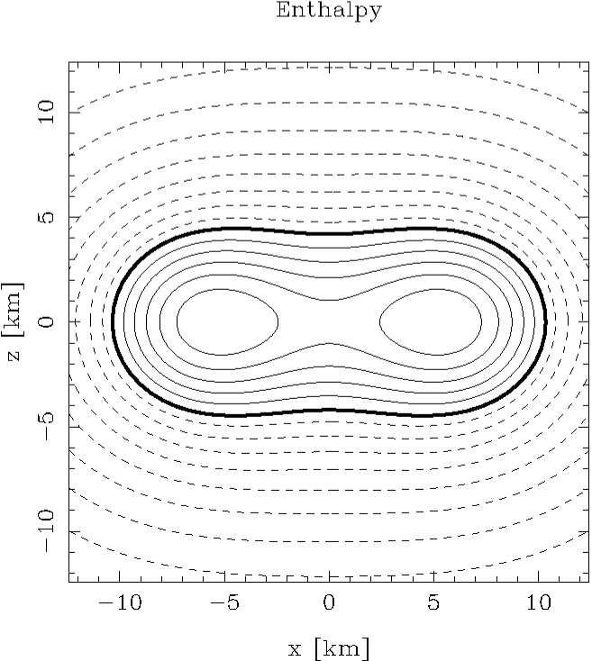
Figure 4: The enthalpy contours in the $(x,z)$ plane for a static star of gravitational mass 2.22 $M_{sol}$ and polar field $8.16\times 10^{17}G$ Chatterjee2015 . The bold line denotes the stellar surface.

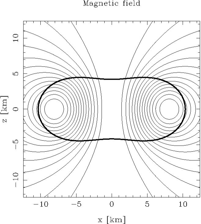
Figure 5: The magnetic field lines for same star as in Fig. 4.

The free physical parameters entering the model are the EoS, the current function $f$ (Eq. 34), the rotation frequency $\Omega$ and the logarithm of the central enthalpy $H_{c}=\log(h(r=0))$. The choice of the current function and the effect of alternative choices has been discussed in  Bocquet . In general relativity, one must define gauge independent quantities in order to derive observables from the numerical models. The gravitational mass $M_{G}$ is defined as the mass perceived by a particle orbiting the star. It may be computed either as the Komar mass (using stationarity) or the ADM mass (asymptotic flatness of space) Gourgoulhon . The baryon mass $M_{B}$ is the product of the baryon mass and total number of baryons in the star. The circumferential equatorial/polar radius $R_{circ}$ can be computed by integrating the line element $ds$ (Eq. 22) over the stellar circumference at the equator or passing through the poles. Detailed definitions and formulae can be found in Refs. Bocquet and BGSM .

5 Effect of magnetised EoS on the structure of strongly magnetised compact stars

5.1 Effect on maximum mass

The effect of the magnetic field on the maximum mass of neutron stars was investigated numerically in several works e.g. Bocquet ; Cardall , assuming different EoSs (from perfect fluid to polytropic to realistic ones). It was found that the effect of the pure electromagnetic field is to increase the maximum mass in neutron stars. For the maximum allowable poloidal magnetic field in  Bocquet , the maximum mass of neutron stars for static stars was found to increase by 13 to 29% (depending on the EoS) with respect to the maximum mass of non-magnetised stars. For rotating configurations, in most cases the magnetic field was found to be more efficient in increasing the maximum mass than the rotation. However such works did not take into account magnetic field modifications of the EoS.

The investigation of the effect of magnetic field dependent EoS on the maximum mass was done for the first time in Chatterjee2015 . The formalism described in Sec. 4 was applied to a magnetised EoS in the mCFL (Magnetic Colour-Flavour-Locked) phase, and the coupled Einstein-Maxwell equations were solved numerically BGSM ; Bocquet . The numerical solution was obtained within the numerical library Lorene Lorene using spectral methods Grandclement as described in Sec. 4.3. The construction of numerical models for isolated rotating neutron stars using this formalism was also discussed in Novak2015 .

It was demonstrated in accordance with earlier results  Bocquet ; Cardall , that on increasing the magnetic field, the Lorentz force exerted by the field deviates the stellar shape more and more from spherical symmetry (see e.g. Fig. 4 and Fig. 5). Fig. 4 also demonstrates the limitation of the code, as the numerical scheme breaks down when the stellar shape is too strongly deformed from spherical to a torus-like form Cardall . This limit is reached when the magnetic pressure at the star’s centre becomes comparable to the fluid pressure and has been numerically explored by Cardall .

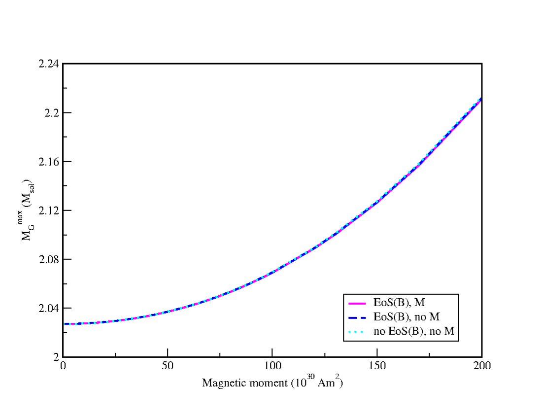
Figure 6: NS maximum mass for models with and without magnetic field dependent EoS and magnetisation

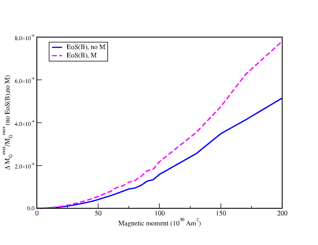
Figure 7: Relative difference in stellar mass for the models in Fig. 6

In Fig. 6 and Fig. 7, NS masses are plotted as a function of the magnetic moment, which is a constant of motion and varies linearly as the stellar magnetic field (see Chatterjee2015 ; Bocquet for discussions). On comparison of the models with and without magnetic field dependent EoS and magnetisation, it was demonstrated in Chatterjee2015 that the relative difference between the maximum masses is negligible if magnetic fields are taken into account consistently in the modelling of magnetars. The same conclusion was also drawn for the variation of the stellar compactness

$$C=\frac{M_{G}}{R_{circ}}$$

as a function of magnetic moment, where $R_{circ}$ is the circumferential equatorial radius BGSM . The effect of anomalous magnetic moment was not included in this work, as its influence on the EoS and global structure is estimated to be small Strickland ; Rabhi . Additional magnetic field effects such as the ferromagnetic instability Maruyama ; Vidaurre or magnetic catalysis Haber , if present in neutron stars, could enhance the effect of magnetic field on the EoS and therefore the maximum mass, too.

5.2 Effect on Radius and Crust-Core properties

Magnetars display a large number of peculiar phenomena, such as anti-glitches, bursts and oscillations that challenge our theoretical understanding of these objects. In Sec. 3.1 we discussed that in the presence of quantising magnetic fields, the motion of charged particles are affected, which in turn, alters the EoS as well as the properties of the crust-core boundary. Moreover, recent studies Pons2013 ; Piekarewicz2014 indicate that the crust-core transition region and the thickness of the crust play an important role during the cooling process of a magnetar and the emission of gravitational waves.

As discussed in the previous section the main influence on the maximum mass of a neutron star in a strong magnetic field does arise from the magnetic pressure itself, the modification of the EoS and magnetisation contributing only marginally for field strength below $10^{19}$ G. From the discussion in Sec. 3.1, we expect only a moderate influence of the magnetic field effects on the EoS on the neutron star radii, too. However, it has been discussed Fang2016 ; Fang2017 that the magnetic field has a non-negligible effect on the dynamical spinodals and hence the crust-core phase transition, which in turn should affect the crust-thickness. This question has been addressed in Fang2016 ; Fang2017 , however, applying the spherically symmetric TOV approximation method to compute the star’s structure, which is not applicable in the presence of a magnetic field.

In ChatterjeeJCAP2019 , the problem was revisited within the framework of density functional theory, using a “Meta-Modelling” technique directly related to the empirical parameters that can be constrained through nuclear physics experiments MM . The numerical formalism described in Sec. 4 was applied to determine the influence of strong magnetic fields on magnetar radii and crust thickness in non-spherical magnetars. First a study of the influence of strong magnetic fields on thermodynamical and dynamical spinodals was performed. The effect of different magnetic field strengths on the thermodynamical spinodals is shown in Figs. 8 and  9. It was concluded that the magnetic field severely modifies the structure of the phase transition region, leading to a non-negligible modifications in the density and pressure of the transition from that of the zero magnetic field case, confirming previous results.

Figure 8: Thermodynamic spinodals for relative magnetic field strength $B_{*}=B/B_{e}^{c}=10^{3}$, with $B_{e}^{c}=4.4\times 10^{13}$ G being the quantising electron field. The continuous red line gives the spinodal envelope in the absence of magnetic field ChatterjeeJCAP2019 .

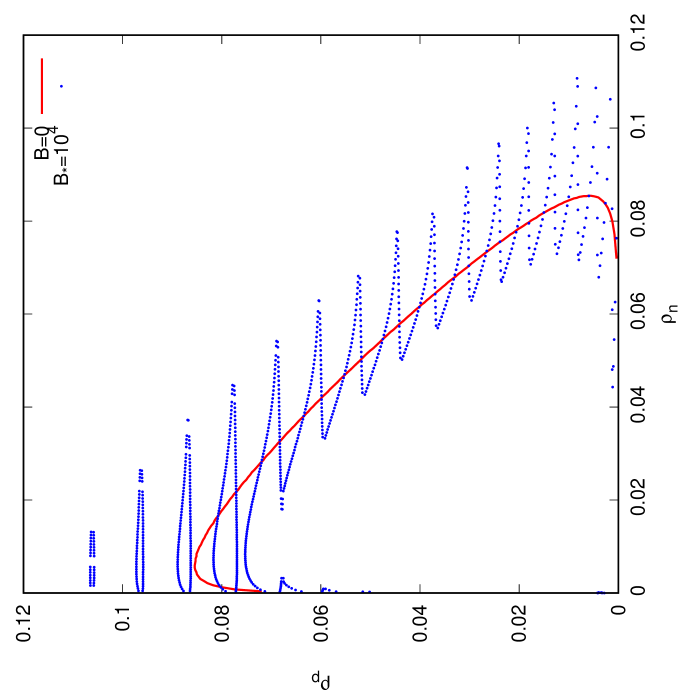
Figure 9: Same as Fig. 8 for relative magnetic field strength $B_{*}=B/B_{e}^{c}=10^{4}$, with $B_{e}^{c}=4.4\times 10^{13}$ G being the quantising electron field  ChatterjeeJCAP2019 .

The effect of magnetic fields on the crust-core phase transition was then studied with a chosen reference Skyrme SLy4 EoS DouchinHaensel , a commonly used EoS in astrophysics. The ideal way to calculate the structure of strongly magnetised neutron stars is to solve the Einstein-Maxwell equations self-consistently with magnetic field dependent EoS, as described in Sec. 4. Employing this method, mass-radius relations of magnetised neutron stars were calculated for full numerical solutions. The unified EoSs for describing both the crust and the core were constructed within the same “Meta-Model” scheme MM ; Chatterjee2017 ; Carreau ; Antic . The magnetic field dependence is only included within the core EoS, assuming a non-magnetised crust. It was demonstrated that the results for previously applied TOV approximation and the fully consistent numerical solutions vary widely due to the different techniques adapted. For low magnetic fields the mass-radius relation resembles closely the zero-field case. With increasing magnetic fields, it departs strongly from the TOV solution. As was already pointed out in Chatterjee2015 ; Chatterjee2017 , this is mainly due to the pure magnetic field contribution and not that of the effect of the magnetised EoS. The other main difference is that for the isotropic TOV calculations, the pure field contribution is a constant, whereas that of the full numerical computation is a profile, generated via a current function. This will be elaborated further in Sec. 6. The model dependence of the results was also tested with two other reference nuclear interaction models, TM1 and Bsk17, and the results obtained were qualitatively similar. It was therefore concluded from this study that a full numerical formalism is inevitable for the calculation of radii and crust thickness strongly magnetised neutron stars.

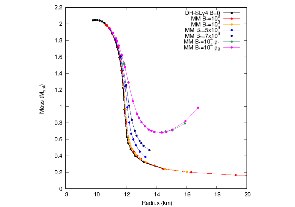
Figure 10: Gravitational mass as a function of circumferential equatorial radius for the SLy4 EoS using full numerical calculation. $B_{*}=B/B_{e}^{c}$, with $B_{e}^{c}=4.4\times 10^{13}$ G being the quantising electron field.

6 Magnetic field distribution

In Sec. 3.1, we already underlined how quantising magnetic fields affect particle populations and their motions. In order to understand how this may affect the nuclear EoS and observable properties such as transport properties, one needs to know the maximum amplitude of the magnetic field at a given depth in the neutron star.

The initial attempts involved assuming an arbitrary magnetic field profile connecting the magnetic field norm $b$ with the surface field $b_{s}$ and the central field $b_{c}$ Bandyopadhyay :

$$b(n_{B}/n_{0})=b_{s}+b_{c}[1-\exp(-\beta(n_{B}/n_{0})^{\gamma})]~{},$$ (39)

with parameters $\beta$ and $\gamma$, chosen to obtain the required values of the maximum field at the centre and at the surface. This profile was subsequently used in more than 100 publications (e.g. Rabhi ; Dexheimer2012 ; Menezes2009a ; Menezes2009b ). An improvement over this formulation was attempted by others, trying to motivate a better choice of parameters Dexheimer2012 ; Lopes2015 ; Dexheimer2017a ; Dexheimer2017b . Lopes and Menezes Lopes2015 introduced a variable magnetic field, depending on the energy density rather than on the baryon number density:

$$b=b_{c}\left(\frac{\epsilon_{M}}{\epsilon_{0}}\right)^{\gamma}+b_{s}~{},$$ (40)

where $\epsilon_{M}$ is the energy-density of the matter contribution, $\epsilon_{0}$ is the central energy density of the maximum mass non-magnetic neutron star and $\gamma$ is a positive chosen parameter, arguing that this formalism reduces the number of free parameters from two to one. This profile was then applied in the calculation of the anisotropic shear stress tensor (see Bednarek ; Menezes2016 ), with the pressure components “averaged” in the form diag$(b^{2}/24\pi,b^{2}/24\pi,b^{2}/24\pi)$ but within a spherically symmetric TOV system. There have also been suggestions of the magnetic field profile being a function of the baryon chemical potential Dexheimer2012 as:

$$b(\mu_{B})=b_{s}+b_{c}\left[1-\exp(\beta\frac{(\mu_{B}-938)^{\alpha}}{938})\right]~{},$$ (41)

with $\alpha=2.5$, $\beta=-4.08\times 10^{-4}$ and $\mu_{B}$ given in MeV. In contrast to the profiles in Eqs. (39,40), such a formula avoids that a phase transition induces a discontinuity in the effective magnetic field. Dexheimer et al. Dexheimer2017a ; Dexheimer2017b also performed a fit to the shapes of the magnetic field profiles in the polar direction as a function of the chemical potentials (as in Dexheimer2012 ) by quadratic polynomials instead of exponential ones as

$$b(\mu_{B})=\frac{(\alpha+\beta\mu_{B}+\gamma\mu_{B}^{2})}{b_{c}^{2}}\mu~{},$$ (42)

where $\alpha,\beta,\gamma$ are coefficients determined from the numerical fit. In Ref. Mallick , a density dependent profile is applied within a perturbative axisymmetric approach similar to the Hartle and Thorne formalism for slowly rotating stars. It remains, however, that the stellar deformation due to the magnetic field implies that such a density (or equivalent) dependent profile should depend on the direction, thus will appear different looking in the polar or the equatorial direction.

It was later demonstrated in MenezesAlloy that such ad hoc field distributions are unphysical, as they do not satisfy Maxwell’s equations. This can also be understood from the fact that assuming such profiles in a spherically symmetric star would incorrectly imply a purely monopolar magnetic field distribution. The ideal way of achieving this would be to solve the coupled Einstein-Maxwell equations described in Sec. 4, provided with a magnetic field dependent EoS. In Chatterjee2019 , a numerical scheme was developed to achieve the above. In order to estimate the value of the magnetic field strength at a given stellar depth to test its potential effect on matter properties, this work provided a “universal” magnetic field strength profile from the surface to the interior obtained from the field distribution in a fully consistent numerical calculation.

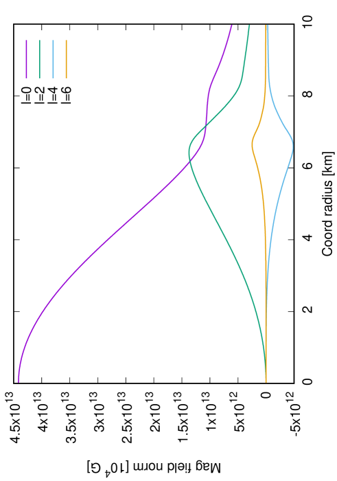
Figure 11: First four even multipoles of the magnetic field norm as functions of the coordinate radius $r$ Chatterjee2019 .

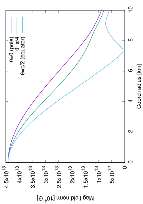
Figure 12: Magnetic field norm as functions of the coordinate radius $r$ for different angular directions ($\theta=0,\pi/4,\pi/2$) Chatterjee2019 .

Using the full numerical solution described in Sec. 4, an extensive investigation of the magnetic field configurations was performed in Chatterjee2019 , for varying mass, magnetic field and EoS. Instead of the magnetic field (which transforms as a vector), a multipolar decomposition of the magnetic field norm (which transforms as a scalar),

$$b(r,\theta)\simeq\sum_{l=0}^{l_{max}}b_{l}(r)\times Y_{l}^{0}(\theta)$$ (43)

was obtained, where $Y_{l}^{m}(\theta,\phi)$ are spherical harmonic functions. The first coefficients $b_{l}$ are displayed in Fig. 11. It was shown (see Fig. 12) that the monopolar (spherically symmetric) term $b_{0}(r)$ is dominant. The profile $b_{0}(r)$ can be fitted by a polynomial as a function of the stellar radius:

$$b_{0}(x)=b_{c}\times(1-1.6x^{2}-x^{4}+4.2x^{6}-2.4x^{8})~{},$$ (44)

where $x=\bar{r}/r_{mean}$ is the ratio of the stellar radius in Schwarzschild coordinates and the mean (or areal) radius. When a neutron star gets distorted from spherical symmetry, it is not possible to define a unique radius, and therefore the description in terms of the Schwarzschild coordinate radius $\bar{r}$ is a convenient one. As evident from Fig. 13, this generic eighth-order polynomial fit applies well for a wide variety of hadronic EoSs (HS(DD2), SFHoY, STOS, BL_EOS, SLy9, SLy230a). It was thus demonstrated that the generic profile for the monopolar component of the magnetic field norm is fairly independent of a wide choice of mass, central magnetic field and hadronic EoSs (with the exception of polytropic and quark matters EoSs), and therefore can be taken as a “universal profile”.

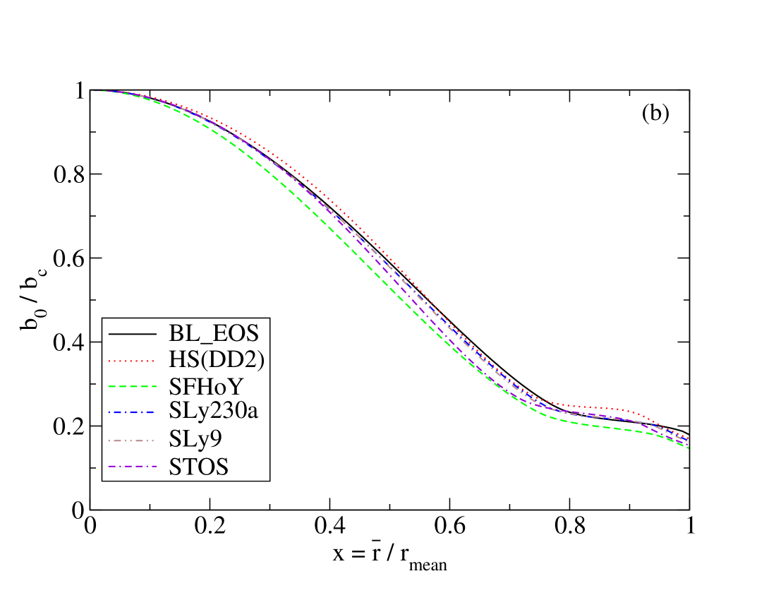
Figure 13: Generic profile for monopolar part of the magnetic field for different EoSs Chatterjee2019 .

This magnetic field profile, derived from realistic computations, can then be applied by nuclear physicists to estimate magnetic field strength inside the neutron star, for studies of its influence on the nuclear composition. As has been shown by Chatterjee et al. Chatterjee2019 , the star’s radius is best determined by solving the simple TOV system (18), thus getting the information needed to use this universal profile.

7 Summary and future prospects

In this review we discussed recent developments in techniques to calculate the global structure of strongly magnetised neutron stars consistently within the general relativistic framework. We explained why isotropic hydrostatic equilibrium equations, used to describe non- magnetised stars, are no longer applicable in presence of an ultrastrong magnetic field that significantly deforms the star. To obtain the global structure, we therefore propose numerically solving equations of stellar equilibrium obtained from conservation of the energy-momentum tensor coupled to Einstein-Maxwell equations Chatterjee2015 . Several of the numerical tools (e.g. Lorene, XNS) are publicly available and have been successfully applied in subsequent works to study global properties of strongly magnetised neutron stars as well as white dwarfs using several realistic equations of state Chatterjee2017b ; Franzon ; Otoniel .

The drawback of the numerical method elaborated in this article and implemented in Lorene is in the choice of the configuration of the magnetic field geometry, as only a purely poloidal configuration is considered. In general also toroidal component in the magnetic field should appear, even with a higher amplitude than the poloidal one, see e.g. Akgun . The effect of purely toroidal fields on the structure of neutron stars was investigated Kiuchi2008 ; Frieben ; KiuchiKotake ; Yasutake ; Yoshida for polytropic EoSs. However the maximum central magnetic field being the same (as estimated from the virial theorem) the effect on the maximum neutron star mass will not be significantly different qualitatively for both configurations. Solutions in mixed toroidal-poloidal configurations have been developed in the Conformally Flat Condition Bucciantini , implemented in the XNS code, and recently, a new code (COCAL) has been obtained for such mixed toroidal-poloidal configurations in the general axisymmetric (and non-circular) spacetimes Uryu .

It was demonstrated as an application of the consistent formalism, how the maximum mass of a neutron star is negligibly modified due to the magnetic field dependence of the microscopic EoS, even for the highest observed neutron star magnetic fields. We also discussed the results of the investigation of the influence of strong magnetic fields on the crust-core phase transition properties, and consequently on the radius and crust thickness of a neutron star ChatterjeeJCAP2019 . It was concluded that large magnetic fields strongly modify the crust-core phase transition. Moreover, a comparison with the results of isotropic TOV models convincingly showed that full numerical solutions are inevitable for the structure of strongly magnetised neutron stars.

We further discussed an application of the full numerical solution in constructing a “universal” magnetic field distribution with radial depth in neutron stars Chatterjee2019 , in place of arbitrary magnetic fields commonly adopted in the literature, to estimate the influence of strong magnetic fields on the NS interior composition. The proposed fit parametrisation, obtained from the full numerical structure calculations, may serve as a useful tool for nuclear physicists.

8 Acknowledgements

D.C. would like to thank Veronica Dexheimer and Constança Providência for kindly providing the data for Figs. 1 and 2 on equations of state in this paper.

References

- (1) R. C. Duncan and C. Thompson, Astrophys. J. 392, L9 (1992)
- (2) V. V. Usov, Nature 357, 472 (1992)
- (3) B. Paczyński, Acta Astron. 42, 145 (1992)
- (4) V. Kaspi and A. M. Belobodorov, Annu. Rev. Astron. Astrophysics 55, 261 (2017)
- (5) F. C. Zelati, N. Rea, J.A. Pons, S. Campana, P. Esposito, Mon. Not. Roy. Astron. Soc. 474, 961 (2018)
- (6) S. B. Popov, R. Turolla and A. Possenti, Mon. Not. Roy. Astron. Soc. 369, L23 (2006)
- (7) H. Tong et al., Res. Astron. Astrophys. 18, 067 (2018)
- (8) S. Ai, H. Gao, Z-G. Dai, X.-F. Wu, A. Li, B. Zhang, Astrophys. J. 860, 57 (2018)
- (9) R. Gill, A. Nathanail, L. Rezzolla, Astrophys. J. 876, 139 (2019)
- (10) W. Fong et al., Astrophys. J. 906, 127 (2021)
- (11) A. I. Ibrahim et al., Astrophys. J. 609, L21 (2004)
- (12) S. Mereghetti, Braz. J. Phys. 43, 356 (2013)
- (13) S. Chandrasekhar and E. Fermi, Astrophys. J. 118, 116 (1953)
- (14) D. Lai and S. L. Shapiro, Astrophys. J. 383, 745 (1991)
- (15) S. Bonazzola and E. Gourgoulhon, Class. Quantum Grav. 11, 1775 (1994).
- (16) E. Gourgoulhon and S. Bonazzola, Class. Quantum Grav. 11, 443 (1994)
- (17) P. Haensel P., A. Y. Potekhin, D.G. Yakovlev, Neutron Stars 1: Equation of state and structure, Springer Berlin (2007)
- (18) D. Chatterjee, I. Vidaña, Eur. Phys. J. A 52,29 (2016)
- (19) L. D. Landau and E. M. Lifshitz, Electrodynamics of continuous media, Pergamon Press (1960)
- (20) V. Canuto and H.-Y Chiu, Phys. Rev. 173, 1210 (1968)
- (21) D. Bandyopadhyay, S. Chakrabarty and S. Pal, Phys. Rev. Lett. 79, 2176 (1997)
- (22) S. Chakrabarty, D. Bandyopadhyay, and S. Pal, Phys. Rev. Lett. 78, 2898 (1997)
- (23) A. Broderick, M. Prakash and J. M. Lattimer, Astrophys. J. 537, 351 (2000)
- (24) A. Broderick, M. Prakash and J. M. Lattimer, Phys.Lett. B 531, 167 (2002)
- (25) M. Strickland, V. Dexheimer and D. P. Menezes, Phys. Rev. C 86, 125032 (2012)
- (26) J. L. Noronha and I. A. Shovkovy, Phys. Rev. D 76, 105030 (2007)
- (27) A. Rabhi, H. Pais, P. K. Panda, C. Providência, J. Phys. G 36, 115204 (2009)
- (28) E. J. Ferrer, V. de la Incera, J. P. Keith, I. Portillo I. and P. L. Springsteen, Phys. Rev. C 82, 065802 (2010)
- (29) M. Sinha, X. G. Huang and A. Sedrakian, Phys. Rev. D 88, 025008 (2013)
- (30) N. Chamel, Zh. K. Stoyanov, L. M. Mihailov, Y. D. Mutafchieva, R. L. Pavlov, and Ch. J.Velchev, Phys. Rev. C 91, 065801 (2015)
- (31) D. Peña-Artega, M. Grasso, E. Khan, P. Ring, Phys. Rev. C 84, 045806 (2011)
- (32) D. Blaschke, N. Chamel, Astrophys. Space Libr. 457, 337 (2018)
- (33) D. G. Ravenhall, C. J. Pethick, and J. R. Wilson, Phys.Rev. Lett. 50, 2066 (1983)
- (34) M. Hashimoto, H. Seki, and M. Yamada, Prog. Theor.Phys. 71, 320 (1984)
- (35) K. Oyamatsu, Nucl. Phys. A 561, 431 (1993)
- (36) C. J. Pethick and D. G. Ravenhall, Ann. Rev. Nucl. Part.Sci. 45,429 (1995)
- (37) G. Watanabe, K. Sato, K. Yasuoka, and T. Ebisuzaki, Phys. Rev. C 68, 035806 (2003)
- (38) S. S. Avancini et al., Phys. Rev. C 78 015802 (2008)
- (39) C. Ducoin, J. Margueron and C. Providência, Eur. Phys. Lett. 91, 32001 (2010)
- (40) S.S. Avancini, S. Chiacchiera, D.P. Menezes and C. Providência, Phys. Rev. C 82, 055807 (2010)
- (41) C. Providência and D.P. Menezes, Phys. Rev. C 96, 045803 (2017)
- (42) J. Fang, S. Avancini, H. Pais and C. Providência, Phys. Rev. C 94, 062801 (2016)
- (43) J. Fang, H. Pais, S. Pratapsi, S. Avancini, J. Li and C. Providência, Phys. Rev. C 95, 045802 (2017)
- (44) H. Pais et al, this issue.
- (45) A. Rabhi, C. Providencia, J. Da Providencia, J. Phys. G 35, 125201 (2008)
- (46) A. Haber, F. Preis and A. Schmitt, Phys. Rev. D 90, 125036 (2014)
- (47) V. Dexheimer, K. D. Marquez, D. P. Menezes, arxiv:2103.09855
- (48) S. Typel, G. Röpke, T. Klähn, D. Blaschke, and H.H. Wolter, Phys. Rev. C 81, 015803 (2010)
- (49) Y. Sugahara, H. Toki, Nucl. Phys. A 579, 557 (1994)
- (50) V. Dexheimer, R. Negreiros and S. Schramm, Eur. Phys. J. A 48, 189 (2012)
- (51) B.C.T. Backes, K.D. Marquez, D.P. Menezes, arxiv:2103.14733.
- (52) D. Kharzeev, K. Landsteiner, A. Schmitt, Ho-ung Yee, Lect. Notes. Phys. 871, 1 (2013)
- (53) R. Gatto and M. Ruggieri, Lect. Notes Phys. 871, 87 (2013)
- (54) E. J. Ferrer and V. de la Incera, Lect. Notes Phys. 871, 399 (2013)
- (55) E. J. Ferrer and A. Hackebill, arxiv:2010.10574
- (56) S. S. Avancini, V. Dexheimer, R. L. S. Farias, and V. S. Timóteo, Phys. Rev. C 97, 035207 (2018)
- (57) D. Chatterjee, T. Elghozi, J. Novak and M. Oertel, Mon. Not. Roy. Astron. Soc. 447, 3785 (2015)
- (58) E. Gourgoulhon, 3+1 Formalism in General Relativity, Lecture Notes in Physics, Springer Verlag (2012)
- (59) L. Paulucci, E. J. Ferrer, V. de La Incera and J. E. Horvath, Phys. Rev. D 83, 043009 (2011)
- (60) V. Dexheimer D. P. Menezes and M. Strickland, J. Phys. G: Nucl. Part. Phys. 41, 015203 (2014)
- (61) R. D. Blandford and L. Hernquist, J. Phys. C 15, 6233 (1982)
- (62) A. Y. Potekhin and D. G. Yakovlev, Phys. Rev. C 85, 039801 (2012)
- (63) L. L. Lopes and D. P. Menezes, Braz. J. Phys. 42, 428 (2012)
- (64) R. Casali, L. B. Castro and D. P. Menezes, Phys. Rev. C 89, 015805 (2014)
- (65) R. L. Bowers and E. P. T. Liang, Astrophys. J. 188, 657 (1974)
- (66) K. Konno, T. Obata, and Y. Kojima, Astron. Astrophys. 352, 211 (1999).
- (67) R. Mallick and S. Schramm, Phys. Rev. C 89, 045805 (2014)
- (68) M. Bocquet, S. Bonazzola, E. Gourgoulhon, J. Novak, Astron. Astrophys. 301, 757 (1995)
- (69) C. Y. Cardall, M. Prakash, J. M. Lattimer, Astrophys. J. 554, 322 (2001)
- (70) K. Kiuchi, S. Yoshida, Phys. Rev. D 78, 044045 (2008)
- (71) A. Oron, Phys. Rev. D 66, 023006 (2002)
- (72) K. Ioka, M. Sasaki, Astrophys. J 600, 296 (2004)
- (73) K. Kiuchi, K. Kotake, Mon. Not. Roy. Astron. Soc. 385, 1327 (2008)
- (74) N. Yasutake, K. Kiuchi, K. Kotake, Mon. Not. Roy. Astron. Soc. 401, 2101 (2010)
- (75) S. Yoshida, K. Kiuchi, M. Shibata, Phys. Rev. D 86, 044012 (2012)
- (76) A.G. Pili, N. Bucciantini and L. Del Zanna, Mon. Not. Roy. Astron. Soc. 439, 3541 (2014)
- (77) S. Bonazzola, E. Gourgoulhon, M. Salgado, J. A. Marck, Astron. Astrophys. 278, 421 (1993)
- (78) J. Frieben, L. Rezzolla, Mon. Not. Roy. Astron. Soc. 427, 3406 (2012)
- (79) R.J. Tayler, Mon. Not. Roy. Astron. Soc. 161,385 (1973)
- (80) P. Markey and R.J. Tayler, Mon. Not. Roy. Astron. Soc. 163, 77 (1973)
- (81) J. Braithwaite, Astron. & Astrophys. 453, 687 (2006)
- (82) J. Braithwaite, Astron. & Astrophys. 469, 275 (2007)
- (83) K. Uryū, S. Yoshida, E. Gourgoulhon, C. Markakis, K. Fujisawa, A. Tsokaros, K. Taniguchi, Y. Eriguchi Phys. Rev. D 100, 123019 (2019)
- (84) T. Akgün, A. Reisenegger, A. Mastrano, and P. Marchant, Mon. Not. Roy. Astron. Soc. 433, 2445 (2013)
- (85) http://www.lorene.obspm.fr
- (86) P. Grandclément and J. Novak, Living Rev. Relat. 12, 1, http://www.livingreviews.org/lrr-2009-1 (2009)
- (87) F. D. Swesty, J. Comp. Phys., 127, 11 (1996)
- (88) J. Novak, M. Oertel, D. Chatterjee and A. Sourie, Proceedings of The Modern Physics of Compact Stars 2015 PoS(MPCS2015) 262, 012 (2016)
- (89) T. Maruyama and T. Tatsumi, Nucl. Phys. A 693, 710 (2001)
- (90) A. Vidaurre, J. Navarro and J. Bernabeu, Astron. Astrophys. 135, 361 (1984)
- (91) J. A. Pons, D. Viganò and N. Rea, Nature Phys. 9, 431 (2013)
- (92) J. Piekarewicz, F. J. Fattoyev and C. J. Horowitz, Phys. Rev. C 90, 015803 (2014)
- (93) D. Chatterjee, F. Gulminelli, and D. P. Menezes, J. Cosmol. Astropart. P 03, 035 (2019)
- (94) J. Margueron, R. Hoffmann Casali and F. Gulminelli, Phys. Rev. C 97 025805 (2018)
- (95) F. Douchin and P. Haensel, A unified equation of state of dense matter and neutron star structure, Astron. Astrophys. 380, 151 (2001)
- (96) D. Chatterjee, F. Gulminelli, A. R. Raduta and J. Margueron, Phys. Rev. C 96, 065805 (2017)
- (97) T. Carreau, F. Gulminelli and J. Margueron, Phys. Rev. C 100, 055803 (2019)
- (98) S. Antic, D. Chatterjee, T. Carreau and F. Gulminelli, J. Phys. G: Nucl. Part. Phys. 46, 065109 (2019)
- (99) D. P. Menezes, M. Benghi Pinto, S. S. Avancini et al., Phys. Rev. C 79, 035807 (2009)
- (100) D. P. Menezes, M. Benghi Pinto, S. S. Avancini and C. Providencia, Phys. Rev. C 80, 065805 (2009)
- (101) L. Lopes and D. Menezes, J. Cosmol. Astropart. Phys. 08, 002 (2015)
- (102) V. Dexheimer, B. Franzon, R. O. Gomes, R. L. S. Farias, S. S. Avancini and S. Schramm, Phys. Lett. B.773, 487 (2017)
- (103) V. Dexheimer, B. Franzon, R. O. Gomes, R. L. S. Farias, S. S. Avancini and S. Schramm, Astronomische Nachrichten 338, 1052 (2017)
- (104) I. Bednarek, A. Brzezina, R. Manka, M. Zastawny-Kubica, Nucl. Phys. A 716, 245 (2003)
- (105) D. P. Menezes and L. Lopes, Eur. Phys. J A 52, 17 (2016)
- (106) D. P. Menezes and M. D. Alloy, arxiv:1607.07687, (2016)
- (107) D. Chatterjee, J. Novak and M. Oertel, Phys. Rev. C 99, 055811 (2019)
- (108) D. Chatterjee, A. F. Fantina, N. Chamel, J. Novak and M. Oertel, Mon. Not. Roy. Astron. Soc. 469, 95 (2017)
- (109) B. Franzon and S. Schramm, Phys. Rev. D 92, 083006 (2015)
- (110) E. Otoniel, B. Franzon, M. Malheiro, S. Schramm and F. Weber, arXiv:1609.05994 (2016)