Using convolutional neural networks for the classification of breast cancer images.

Abstract

In this study I compare different architectures of convolutional neural networks and different hardware acceleration devices for the detection of breast cancer from microscopic images of sentinel lymph nodes tissue. Convolutional models with increasing depth are trained and tested on a public data set of more than 300,000 images of lymph node tissue, on four different hardware acceleration cards, using an off–the–shelf deep learning framework. The impact of transfer learning, data augmentation and hyperparameters fine-tuning are also tested. Hardware acceleration device performance can improve training time by a factor of five to twelve, depending on the model used. On the other hand, increasing convolutional depth will augment the training time by a factor of four to six times, depending on the acceleration device used. Increasing the depth of the model, as could be expected, clearly improves performance, while data augmentation and transfer learning do not. Fine-tuning the hyperparameters of the model notably improves the results, with the best model showing a performance comparable to state–of–the–art models.

Introduction

Pathologists have been making diagnoses using digital images of glass microscope slides for many decades. In recent years, advances in slide scanning techniques has allowed the full digitization of microscopic stained tissue sections. There are many advantages to the digitalization of such images, including standardization, reproducibility, the ability to create workflows, remote diagnostics, immediate access to archive, easier sharing among expert pathologists [1]. Breast cancer is the leading cancer type in women worldwide, with an estimated 2 million new cases and 627,000 deaths in 2018. Breast cancer staging refers to the process of describing the tumor growth or spread. Accurate staging by pathologists is an essential task that will determine the patient’s treatment and his chances of recovery (prognosis). An important part of breast cancer staging is the assessment of the sentinel axillary node, a tissue commonly used for the detection of early signs of tumor spreading (metastasis). However, sentinel lymph nodes assessment by pathologists is not always easy and optimal. For instance, a retrospective survey performed in 2012 by expert pathologists requalified the status of a high proportion of sentinel nodes [2]. Deep learning algorithms have made major advances relatively recently in solving problems that have resisted the machine learning and artificial intelligence community such as speech recognition, the activity of potential drug molecules, brain circuits reconstruction and the prediction of the effects of non-coding RNA mutation on gene expression and disease [3]. Convolutional neural networks (CNNs) are a class of deep neural networks characterized by a shared-weight architecture of convolution kernels (or filters) that slide along input features and provide translation equivariant features known as feature maps. One of the main advantages of CNNs is that the network learns to optimize the filters through automated learning, requiring very little pre-processing compared to other machine learning techniques. Since their introduction in the 1990’s [4], CNNs have shown excellent performances in the most challenging visual classification tasks and are currently dominating this research field [5]. When applied to medical imaging, CNNs demonstrated excellent performance and have been successfully used for the identification of retinal diseases from fundus images [6, 7, 8], tuberculosis from chest radiography images [9, 10] and malignant melanoma from skin images [11]. CNNs have also been used for the detection of lymph node metastases in women with breast cancer in an algorithm competition known as CAMELYON16 (Cancer Metastases in Lymph Nodes Challenge), with the best models showing equal or slightly better performances than a panel of pathologists [12]. In this study, I use a data set of more than 300,000 lymph node images derived from CAMELYON, known as the PCam (Patch CAMELYON) data set [13] to characterize and analyze the performance of different CNNs network architectures and GPU accelerators, using a standard, off–the–shelf, deep learning computational library.

Material and methods

The PCam data set was downloaded from the original website (https://github.com/basveeling/pcam). All images have a size of 96 x 96 pixels, in three colors. The training set has 262,144 images (80 % of the total), the validation set has 32,768 images (10 %) and the test set has also 32,768 images (10 %). All data sets have a 50/50 balance between positive (tumor present) and negative (tumor absent) samples.

All models were coded in Python (v3.7.5) using the TensorFlow (v2.4.1) and integrated Keras API (v2.4.0). Some additional statistics and performance indicators were calculated with the Sci-Kit Learn Python package [14]. The model performance was tested on three different GPU architectures: Nvidia Tesla K80 with 32 Gb of RAM, Nvidia Pascal P100 with 16 Gb of RAM, Nvidia Volta V100 with 32 Gb of RAM and Nvidia Ampere A100 with 80Gb of RAM . All the models tested in this study, including the code for tuning some of the models, are available on GitHub (https://github.com/erbon7/pcam_analysis).

For each network architecture tested in this study, the same procedure is used: the model is trained on the training set for 15 epochs, with an evaluation on the validation set after each epoch. Depending on the accurracy value of the model, the weights are saved after each epoch to keep the best model, which is then evaluated on the test set. For some models, I used the KerasTuner framework with the Hyperband algorithm to optimize some hyperparameters [15]. For the CNN-2L and CNN-6L models, the batch size, the size of the dense layer and the learning rate were optimized. For the IV3-F model, only the learning rate and batch size were optimized.

Results

Figure 1: Normal and tumor example images from the PCam data set. The red rectangle corresponds to the 32 x 32 pixels center. The presence of at least one pixel of tumor tissue in this region dictates a positive label (1), otherwise the image is labeled as negative(0).

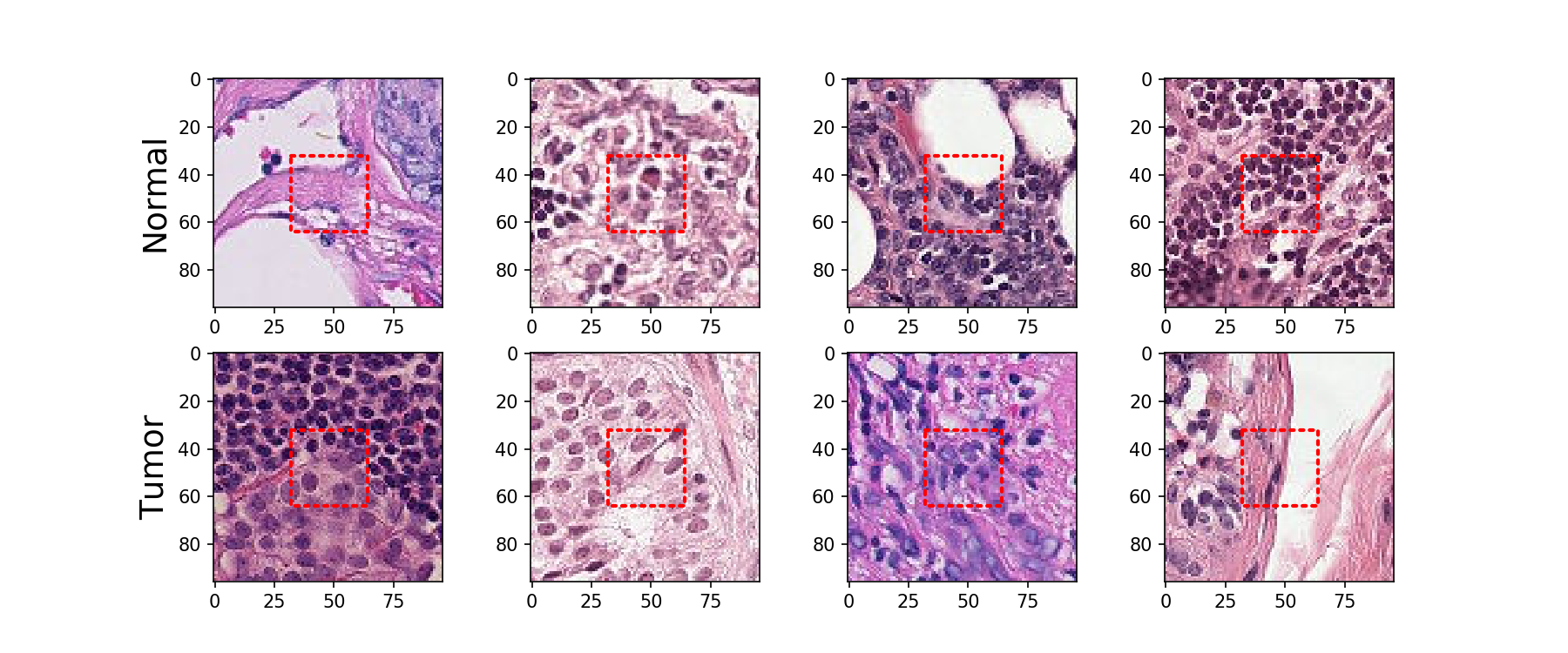
In the CAMELYON16 challenge [12], hundreds of whole-slide images of sentinel lymph nodes sections with or without nodal metastases verified by standard immunohistochemical staining by expert pathologists are provided to the participants to build algorithms. The PCam data set is composed of patches of 96 x 96 pixels images automatically extracted from the CAMELYON data set [13]. For each image, a positive label indicates that the 32 x 32 pixel center of the image contains at least one pixel annotated as tumor tissue (Figure 1).

Figure 2: Simplified architecture of the CNN-2L (a, two convolutional layers) and CNN-6L (b, six convolutional layers) models.

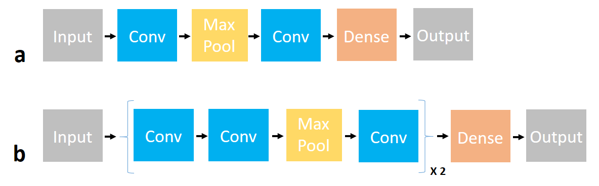
Three different CNN models were used in this study, with different depth levels (Table 1). The first model (CNN-2L) is very simple with only two convolutional layers (Figure 2a). This model was trained with a batch size of 32, the Adam gradient optimizer [16] with default rate 1e-3, a final dense layer of 256 nodes and a training epoch number of 15. The second model (CNN-6L) is more deep and complex with six convolutional layers (Figure  2b). It is trained with the same parameter values as the CNN-2L. The architecture for the CNN-6L model was inspired by the Kaggle models of F. Marazzi (https://bit.ly/35wINGv) and H. Mello (https://bit.ly/3xwI6cl). Note that the CNN-6L model include batch normalization [17] and dropout steps to improve performance.

Table 1: CNN models.

Model name	Description
CNN-2L	Simple model with 2 convolutional layers
CNN-6L	Deep model with 6 convolutional layers
IV3	InceptionV3 [18] very deep convolutional model,
	with (IV3-TL) or without (IV3-F) transfer learning.

The last model is InceptionV3, a model created in 2015 with a very deep architecture (94 convolutional layers) that performs very well on various computer vision tasks [18], such as the the ImageNet challenge (https://image-net.org/challenges/LSVRC/), a competition with hundreds of object categories and millions of images [19]. The InceptionV3 model is available in the TensorFlow Keras as part of some ”standard” deep learning models included in this library. Furthermore, it is possible to load the model pre-weighted with ImageNet training weights, thus enabling transfer learning (TF). TF is a popular approach in deep learning where pre-trained models are used as the starting point on computer vision and natural language processing tasks in order to save computing and time resources. Here I have used the InceptionV3 model both pre-trained with imagenet weights (IV3-TL) and fully re-trained (IV3-F) with the PCam data sets. For the pre-trained version, only the last layers of the model are re-trained with the PCam data set (global average pooling layer, dense layer and final output). Of course, given that the number of training parameters is much greater in the case of the fully re-trained InceptionV3 model, the computation time needed for training the model is also expected to be much longer. Table 2 is detailing the architecture and parameters for each of the models used in this study.

Table 2: CNN models architecture and parameters.

	CNN-2L	CNN-6L	IV3-TL	IV3-F
Number of convolutional layers	2	6	94	94
Total number of parameters	9.5M	2.4M	22M	22M
Number of training parameters	9.5M	2.4M	524K	22M
Batch size	32	32	32	32
Dense layer size	256	256	256	256

The computational running time for the different models is detailed in Table 3. Note that the time corresponds to the average time observed for one epoch. We can compare the model architecture and the hardware GPUs acceleration for the PCam data set analysis. As expected, the running time is increasing with the complexity and depth of the model. The IV3-F model is taking 4 to 6 times longer to train than the simple 2 convolutional layers CNN-2L model, depending on the GPU card model. The 6 layers CNN model is taking 1.7 to 2 times longer than the 2 layers CNN to train. With the InceptionV3 model, using transfer learning is obviously saving a lot of training time, as a full model training is taking $\sim$3 times longer to train on all GPU models. In fact, even though the IVF-TL model (transfer learning) is much more complex, the running time is comparable to the 2 and 6-layers models. Regarding the different GPU cards tested here, more recent and powerful GPU cards decrease the computing time quite drastically, with an acceleration factor between 5 and 12 times for the most recent architecture tested here (A100) on all the CNN models compared to the oldest model tested here (K80). It is worth noticing that the deepest model tested here can be fully trained in about one hour with a V100 or A100 GPU card.

Table 3: Run time in seconds for one epoch on different GPU architectures. NbCU: number of CUDA cores. Pp: processing power in GFlops.

GPU card	NbCU	Pp	CNN-2L	CNN-6L	IV3-TL	IV3-F
K80 (2014)	4992	2400	325	562	468	1333
P100 (2016)	3584	5000	70	121	143	393
V100 (2017)	5120	7000	47	78	98	279
A100 (2020)	6912	8000	26	57	100	270

The performance of all the models on the PCam data set is described in Table 4. All the indicators are measured on the test set. A global improvement of the performances is quite clearly associated with an increased depth of the models. For instance the AUC of the simple 2-layers convolutional model is 0.85, increasing to 0.91 with the 6-layers convolutional model. The InceptionV3 model, which has 94 convolutional layers, also has an AUC of 0.91. Transfer learning does not work very well, since the AUC of the InceptionV3 model trained with the ImageNet weights is only 0.88, better than the 2 convolutional layers model but worse than the 6 convolutional layers (0.91) and the InceptionV3 fully re-trained (0.91). It might be that the visual structures (i.e. the filters) learned with the ImageNet data set are not adapted to the PCam images. Object categories in the ImageNet data set (such as ”ballon”, ”strawberry”, etc.) are indeed very different from the type and structures seen on lymph node tissue microscopy images. Image data augmentation is a technique that can be used to artificially expand the size of a training data set by creating modified versions of the images. This technique was used for the CNN-6L model, but with no obvious positive result on the performance (test loss 0.70, test accuracy 0.73, AUC 0.90). We can see in the table that fine-tuning models is improving performance for both the 6 convolutional layers model (AUC 0.92) and the InceptionV3 fully re-trained model (AUC 0.954). The performance of the fined-tuned InceptionV3 model fully re-trained (IV3-F) is comparable to current state–of–the–art models for computational pathology analysis. It is within the top 5 best algorithms of the CAMELYON16 challenge [12] and is within the top 10 best models for the PCam dataset (https://paperswithcode.com/sota/breast-tumour-classification-on-pcam). The current best PCam models have an AUC around 0.97 and implement rotation equivariant strategies [20, 21, 22]. Indeed, histology images are typically symmetric under rotation, meaning that each orientation is equally as likely to appear. Rotation–equivariance removes the necessity lo learn this type of transformation from the data, thus allowing more discriminative features to be learned and also reducing the number of parameters of the model.

Table 4: Performance of the models on the PCam test set. Tn CNN-6L: fine-tuned version of the CNN-6L model. Tn IV3-F: fine-tuned version of the IV3-F model. AUC: area under the ROC curve.

Metric	CNN-2L	CNN-6L	IV3-TL	IV3-F	Tn CNN-6L	Tn IV3-F
Loss	0.47	0.44	0.46	0.42	0.45	0.32
Accuracy	0.78	0.84	0.78	0.84	0.85	0.89
AUC	0.85	0.91	0.88	0.91	0.92	0.95

References

- [1] Jon Griffin and Darren Treanor. Digital pathology in clinical use: where are we now and what is holding us back? Histopathology, 70(1):134–145, 2017.
- [2] JHMJ Vestjens, MJ Pepels, Maaike de Boer, George Florimond Borm, Carolien HM van Deurzen, Paul J van Diest, JAAM Van Dijck, EMM Adang, Johan WR Nortier, EJ Th Rutgers, et al. Relevant impact of central pathology review on nodal classification in individual breast cancer patients. Annals of Oncology, 23(10):2561–2566, 2012.
- [3] Yann LeCun, Yoshua Bengio, and Geoffrey Hinton. Deep learning. Nature, 521(7553):436–444, 2015.
- [4] Yann LeCun, Bernhard Boser, John S Denker, Donnie Henderson, Richard E Howard, Wayne Hubbard, and Lawrence D Jackel. Backpropagation applied to handwritten zip code recognition. Neural computation, 1(4):541–551, 1989.
- [5] Matthew D Zeiler and Rob Fergus. Visualizing and understanding convolutional networks. In European conference on computer vision, pages 818–833. Springer, 2014.
- [6] Daniel Shu Wei Ting, Carol Yim-Lui Cheung, Gilbert Lim, Gavin Siew Wei Tan, Nguyen D Quang, Alfred Gan, Haslina Hamzah, Renata Garcia-Franco, Ian Yew San Yeo, Shu Yen Lee, et al. Development and validation of a deep learning system for diabetic retinopathy and related eye diseases using retinal images from multiethnic populations with diabetes. Jama, 318(22):2211–2223, 2017.
- [7] Daniel S Kermany, Michael Goldbaum, Wenjia Cai, Carolina CS Valentim, Huiying Liang, Sally L Baxter, Alex McKeown, Ge Yang, Xiaokang Wu, Fangbing Yan, et al. Identifying medical diagnoses and treatable diseases by image-based deep learning. Cell, 172(5):1122–1131, 2018.
- [8] Philippe M Burlina, Neil Joshi, Michael Pekala, Katia D Pacheco, David E Freund, and Neil M Bressler. Automated grading of age-related macular degeneration from color fundus images using deep convolutional neural networks. JAMA ophthalmology, 135(11):1170–1176, 2017.
- [9] Paras Lakhani and Baskaran Sundaram. Deep learning at chest radiography: automated classification of pulmonary tuberculosis by using convolutional neural networks. Radiology, 284(2):574–582, 2017.
- [10] Daniel SW Ting, Paul H Yi, and Ferdinand Hui. Clinical applicability of deep learning system in detecting tuberculosis with chest radiography. Radiology, 286(2):729–731, 2018.
- [11] Andre Esteva, Brett Kuprel, Roberto A Novoa, Justin Ko, Susan M Swetter, Helen M Blau, and Sebastian Thrun. Dermatologist-level classification of skin cancer with deep neural networks. nature, 542(7639):115–118, 2017.
- [12] Babak Ehteshami Bejnordi, Mitko Veta, Paul Johannes Van Diest, Bram Van Ginneken, Nico Karssemeijer, Geert Litjens, Jeroen AWM Van Der Laak, Meyke Hermsen, Quirine F Manson, Maschenka Balkenhol, et al. Diagnostic assessment of deep learning algorithms for detection of lymph node metastases in women with breast cancer. Jama, 318(22):2199–2210, 2017.
- [13] Bastiaan S Veeling, Jasper Linmans, Jim Winkens, Taco Cohen, and Max Welling. Rotation equivariant cnns for digital pathology. In International Conference on Medical image computing and computer-assisted intervention, pages 210–218. Springer, 2018.
- [14] Fabian Pedregosa, Gaël Varoquaux, Alexandre Gramfort, Vincent Michel, Bertrand Thirion, Olivier Grisel, Mathieu Blondel, Peter Prettenhofer, Ron Weiss, Vincent Dubourg, et al. Scikit-learn: Machine learning in python. the Journal of Machine Learning Research, 12:2825–2830, 2011.
- [15] Tom O’Malley, Elie Bursztein, James Long, François Chollet, Haifeng Jin, Luca Invernizzi, et al. Keras tuner. https://github.com/keras-team/keras-tuner, 2019.
- [16] Diederik P Kingma and Jimmy Ba. Adam: A method for stochastic optimization. arXiv preprint arXiv:1412.6980, 2014.
- [17] Sergey Ioffe and Christian Szegedy. Batch normalization: Accelerating deep network training by reducing internal covariate shift. In International conference on machine learning, pages 448–456. PMLR, 2015.
- [18] Christian Szegedy, Vincent Vanhoucke, Sergey Ioffe, Jon Shlens, and Zbigniew Wojna. Rethinking the inception architecture for computer vision. In Proceedings of the IEEE conference on computer vision and pattern recognition, pages 2818–2826, 2016.
- [19] Olga Russakovsky, Jia Deng, Hao Su, Jonathan Krause, Sanjeev Satheesh, Sean Ma, Zhiheng Huang, Andrej Karpathy, Aditya Khosla, Michael Bernstein, Alexander C. Berg, and Li Fei-Fei. ImageNet Large Scale Visual Recognition Challenge. International Journal of Computer Vision (IJCV), 115(3):211–252, 2015.
- [20] Taco Cohen and Max Welling. Group equivariant convolutional networks. In International conference on machine learning, pages 2990–2999. PMLR, 2016.
- [21] Simon Graham, David Epstein, and Nasir Rajpoot. Dense steerable filter cnns for exploiting rotational symmetry in histology images. IEEE Transactions on Medical Imaging, 39(12):4124–4136, 2020.
- [22] Maurice Weiler, Fred A Hamprecht, and Martin Storath. Learning steerable filters for rotation equivariant cnns. In Proceedings of the IEEE Conference on Computer Vision and Pattern Recognition, pages 849–858, 2018.