Boosting the Conformational Sampling by Combining Replica Exchange with Solute Tempering and Well-Sliced Metadynamics

Abstract

Methods that combine collective variable (CV) based enhanced sampling and global tempering approaches are used in speeding-up the conformational sampling and free energy calculation of large and soft systems with a plethora of energy minima. In this paper, a new method of this kind is proposed in which the well-sliced metadynamics approach (WSMTD) is united with Replica Exchange with Solute Tempering (REST2) method. WSMTD employs a divide-and-conquer strategy wherein high-dimensional slices of a free energy surface are independently sampled and combined. The method enables one to accomplish a controlled exploration of the CV-space with a restraining bias as in umbrella sampling (US), and enhance-sampling of one or more orthogonal CVs using a metadynamics (MTD) like bias. The new hybrid method proposed here enables boosting the sampling of more slow degrees of freedom in WSMTD simulations, without the need to specify associated CVs, through a replica exchange scheme within the framework of REST2. The high-dimensional slices of the probability distributions of CVs computed from the united WSMTD and REST2 simulations are subsequently combined using the weighted histogram analysis method (WHAM) to obtain the free energy surface. We show that the new method proposed here is accurate, improves the conformational sampling, and achieves quick convergence in free energy estimates. We demonstrate this by computing the conformational free energy landscapes of solvated alanine tripeptide and Trp-cage mini protein in explicit water.

I Introduction

Molecular dynamics (MD) simulations are widely used to study conformational sampling of large biological systems, compute free energetics and identify the mechanism of biochemical processes.Karplus_McCommon:Nat:2002 ; Schulten:2009 ; Dshaw:Science:2010 ; Shaw:ARB:2012 Modelling large biological systems pose several challenges, primarily due to large number of conformational states and significant energetic and entropic barriers separating different conformational states.Schulten:2009 Advanced enhanced sampling techniques are quintessential for achieving proper sampling of conformational states and obtaining reliable free energy estimates.Chipot:07 ; Vanden:2009:jcc ; Tuckerman:Book ; vanGunsteren:JCC:Rev:2010 ; Ciccotti:12 ; Giovanni:Entropy:2014 ; Pratyush:2016 ; McCammon:2016 ; Pietrucci:2017 ; Peters:Book ; shalini:review:2019 ; vashisth:review:2019 It is a common practice to use either CV-based or global tempering-based enhanced sampling techniques in combination with MD simulations to improve the sampling. These approaches are applied to a variety of problems including protein folding/unfolding, protein-drug binding/unbinding, transport of molecules through membranes, protein aggregation etc.Adam:AR:2007 ; Daniel:AR:2011 ; Wingbermuhle:2020 ; Acharya:2021

Biased sampling, generalized-ensemble or global tempering, and the combination of the both form the three major classes of enhanced sampling methods. Generalized-ensemble methods achieve a random walk in configurational space by accelerating all the degrees of the freedom either by increasing the temperature of the system or by scaling-down the potential energy. Several methods in this category use the replica exchange molecular dynamics (REMD)remd:1999 algorithm. Methods such as parallel temperingremd:1999 , replica exchange solute tempering (REST),rest:2005 and the modified version of REST, called REST2rest2:2011 , belong to this family. Recently modified versions of REST method have been proposed for improving the sampling.Sugita:JCP:2018 ; REHT:2021 Some other distinct global tempering methods are accelerated molecular dynamics(aMD),amd:2004 chemical floodingchemical_flooding:1995 , integrated tempering sampling.ITS:2004 and accelerated weight histogram method (AWH).AWH:2014 ; AWH-1:2021

In other family of methods, enhanced sampling of certain geometric variables of the system, called collective variables (CVs), are carried out by adding a bias potential along CVs or by enhancing the temperature of CVs. Umbrella sampling (US),us:1974 ; us:1977 metadynamics (MTD),mtd:2002 adaptive biasing force methodDarve:2001 , logarithmic mean-force dynamics (LogMFD),LogMFD:2012 driven-Adiabatic Free Energy Dynamics/Temperature Accelerated Molecular Dynamics (d-AFED/TAMD)tamd:1 ; tamd:2 , Variational Enhanced SamplingVariational:1 and other variantswt-mtd:2008 ; be:mtd:1 ; pbmtd:2015 ; shalini:2016 are some examples of biased sampling methods. Such methods require a priori selection of a set of CVs that describes the process of interest. The accuracy of the properties computed from the explored conformational ensemble may depend on the quality of the chosen CVs. Identification of optimal CVs is a challenging task.Frank_Noe:2017 ; Henkelman:2017 ; VPande:2018 ; Gerhard:2018 Inclusion of large number of CVs for biased sampling is often required for an efficient exploration of the CV-space and for quick convergence in free energy estimates. The efficiency of most of the aforementioned biased-sampling techniques diminishes with increasing dimensionality of the CV-space. Sampling of high dimensional free energy landscapes requires advanced techniques such as d-AFED/TAMD,tamd:1 ; tamd:2 bias-exchange MTD,be:mtd:1 parallel-bias MTD,pbmtd:2015 unified-free energy dynamics,ufed:2012 and temperature accelerated sliced samplingtass:2017 .

To take the best out of both the generalized ensemble and the CV based biased-sampling methods, hybrid sampling algorithms are proposed. Replica exchange umbrella sampling (REUS),reus:2013 replica exchange with CV tempering,rect:2015 combination of parallel tempering with MTD,ptmtd:2006 ; reus-rest replica state exchange MTD,rse-mtd:2015 and multi-scale sampling using temperature accelerated and REMDmustar-MD are examples of such methods. It has been observed that for modelling protein folding/unfolding and protein-drug binding/unbinding, these methods are advantageous.ptmtd:2006 ; rect:2015 ; reus-rest ; reus:2013 ; Applications:1 ; Application:2 ; Application:3 ; Application:4 ; Application:REDS:2021

In this paper, we introduce a new method called globally accelerated sliced sampling (GASS) by integrating the WSMTD and REST2 approach. WSMTDshalini:2016 was introduced by our group for increasing the efficiency of MTD method by driving the bias along a specific direction and by controlling the span of the explored CV-space. This method is suited to study systems with broad, flat and unbound free energy landscapes. This method has been applied to study various problemsApplication:wsmtd:2017 ; Application:wsmtd:2018_1 ; Application:2018:2 ; Application:wsmtd:2020:1 ; Application:wsmtd:2020:2 ; Application:wsmtd:2021 and has also been extended to deal with high-dimensional CV-space.tass:2017 By combining REST2 with WSMTD, we hope to boost the sampling of hidden transverse coordinates while exploring the relevant CV space. The controlled biased sampling feature of WSMTD could thus be extended to the conformational sampling of large biomolecular systems in solution and is expected to be beneficial for studying problems like protein folding.

Here, we first introduce the theory behind the GASS method. Subsequently, we present the results of two applications using the GASS method: computation of conformational free energy landscapes for (a) alanine tripeptide, and (b) Trp-cage mini protein in water.

II Methods

WSMTD is a CV based enhance sampling method which can help to achieve a controlled exploration of the CV space by combining US and MTD. While US is ideal for a controlled or directional sampling along one CV, MTD is advantageous in sampling orthogonal CVs in a self guided manner. In WSMTD, our interest is in computing an $n$-dimensional free energy surface $F(\mathbf{s}$) as a function of CVs, $\mathbf{s}(\mathbf{R})\equiv\{s_{1},\cdots,s_{n}\}$, where $\mathbf{R}$ is the set of atomic coordinates. WSMTDshalini:2016 uses the Lagrangian,

$$\mathcal{L}_{h}^{\rm ws}(\mathbf{R},\dot{\mathbf{R}})=\mathcal{L}^{0}(\mathbf{R},\dot{\mathbf{R}})-W^{\rm b}_{h}(s_{1})-V^{\rm b}({\overline{\mathbf{s}}},t),$$ (1)

$h=1,...,M$, where, $\mathcal{L}^{0}$ is the unbiased Lagrangian, $\dot{\mathbf{R}}$ is the set of velocities, and ${\overline{\mathbf{s}}}\equiv\left\{s_{2},\cdots,s_{n}\right\}$.

In WSMTD, we apply a restraining bias

$$W^{\rm b}_{h}(s_{1})=\frac{1}{2}k_{h}(s_{1}-z_{h})^{2}$$ (2)

placed at $s_{1}=z_{h}$. The parameter $k$ determines the curvature of the biasing potential at $h^{\rm th}$ window. Here, $M$ umbrella windows placed from $z_{1}$ to $z_{M}$ along $s_{1}$ define the span of sampling of that CV. This helps in achieving a controlled sampling of the coordinate $s_{1}$, similar to the conventional US technique. In WSMTD, we also apply a well-tempered MTD bias potential

$$V^{\rm b}({\overline{\mathbf{s}}},t)=\sum_{\tau<t}w_{\tau}\exp\left[-\frac{\left({\overline{\mathbf{s}}}-{\overline{\mathbf{s}}}(\tau)\right)^{2}}{2(\delta s)^{2}}\right]\enspace,$$ (3)

in order to sample the orthogonal coordinates ${\overline{\mathbf{s}}}$. Here, $\delta s$ is the width parameter defining the Gaussian potential and

$$w_{\tau}=w_{0}\exp\left[-\frac{V^{\rm b}({\overline{\mathbf{s}}},t)}{k_{\rm B}\Delta T}\right]\enspace,$$ (4)

Where $w_{0}$ is the Gaussian height parameter, $k_{\rm B}$ is the Boltzmann constant, and $\Delta T$ is a tempering parameter.

The free energy surface, $F(\mathbf{s})$, is reconstructed from the probability distribution, $P(\mathbf{s})$, of the CVs as,

$$F(\mathbf{s})=-\frac{1}{\beta}\ln P(\mathbf{s})$$ (5)

where $\beta=(k_{\rm B}T)^{-1}$. In order to obtain $P(\mathbf{s})$, a time independent probability distribution, $P_{h}^{\rm u}(\mathbf{s})$, is obtained by reweighting the MTD time-dependent bias potential as,

$$P^{\rm u}_{h}(\mathbf{s}^{\prime})=\frac{\int_{t_{\rm min}}^{t_{\rm max}}d\tau\,\exp\left[\beta\{V^{\rm b}({\overline{\mathbf{s}}},\tau)-c(\tau)\}\right]\prod_{\alpha=1}^{n}\delta(s_{\alpha}(\tau)-s_{\alpha}^{\prime})}{\int_{t_{\rm min}}^{t_{\rm max}}d\tau\,\exp\left[\beta\{V^{\rm b}({\overline{\mathbf{s}}},\tau)-c(\tau)\}\right]}\enspace,$$ (6)

for each umbrella window $h$. In the above, $c(t)$ is evaluated asTiwary-Parinello:2015

$$c(t)=\frac{1}{\beta}\ln\left[\frac{\int d{\overline{\mathbf{s}}}\exp[-\beta\gamma V^{\rm b}({\overline{\mathbf{s}}},t)]}{\int d{\overline{\mathbf{s}}}\exp[-\beta(\gamma-1)V^{\rm b}({\overline{\mathbf{s}}},t)]}\right]$$ (7)

and $\gamma={(T+\Delta T)}/{\Delta T}$ . Now we employ the weighted histogram analysis method (WHAM)wham:1 ; wham:2 to combine the distributions $P^{\rm u}_{h}(\mathbf{s})$, $h=1,\cdots,M$ and reweight the restraining bias by self-consistent calculations using,

$$P(\mathbf{s})=\frac{\sum^{M}_{h=1}n_{h}P^{\rm u}_{h}(\mathbf{s})}{\sum_{h=1}^{M}n_{h}\exp[\beta f_{h}]\exp[-\beta W_{h}^{\rm b}(s_{1})]}$$ (8)

and

$$\exp[-\beta f_{h}]=\int d\mathbf{s}\,\exp\left[-\beta W_{h}^{\rm b}(s_{1})]\,P(\mathbf{s})\right]\enspace.$$ (9)

In the above, $n_{h}$ is the number of configurations sampled in the $h^{\rm th}$ umbrella window.

In the REST2 method,rest:2005 ; rest2:2011 the potential energies of a selected set of atoms in each replica are scaled-down by some parameter $\lambda$ to enhance their sampling, and conformations sampled in these scaled-replica are exchanged with the non-scaled replica to improve the conformational sampling of the latter. The atoms which are part of the scaled-potential terms (in a molecular mechanics force-field) are referred to be in “hot” region and the rest are said to be in “cold” region. Pair-wise potential form of the molecular mechanics force-field makes it easier to selectively scale potential contributions for a set of atoms and differently scale torsional, electrostatics, and Lennard-Jones terms. Typically, for a solvated protein system, the potential energy of a replica $m$ is computed from the modified contributions of the protein-protein (pp), protein-water (pw) and water-water (ww) interactions, as

$$U_{m}^{\rm REST2}({\bf{R}})=\lambda_{m}\,U_{\rm pp}({\bf{R}})+\sqrt{\lambda_{m}}\,U_{\rm pw}({\bf{R}})+U_{\rm ww}({\bf{R}}),$$

$m=0,\cdots,N_{\rm r}-1$, where $\lambda_{m}={\beta_{m}}/{\beta_{0}}$, $N_{\rm r}$ is the number of replicas, and $\beta_{m}>\beta_{0}$. The $\beta_{m}$ parameter is set different for different replicas. For $m=0$, i.e., for the unscaled replica, we take $\beta_{0}=(k_{\rm B}T_{0})^{-1}$, where $T_{0}$ is the physical temperature of the system. Exchange between adjacent replicas is attempted by swapping their atomic coordinates based on the Metropolis exchange criterion

$$p(i\rightarrow j)=\min(1,e^{-\Delta_{i,j}})\enspace,$$ (10)

with

$$\Delta_{i,j}=(\beta_{i}-\beta_{j})\left[(U_{\rm pp}({{\mathbf{R}}_{j}})-U_{\rm pp}({{\mathbf{R}}_{i}}))+\frac{\sqrt{\beta_{0}}}{\sqrt{\beta_{i}}+\sqrt{\beta_{j}}}(U_{\rm pw}({\mathbf{R}_{j}})-U_{\rm pw}({\mathbf{R}_{i}}))\right]\enspace.$$ (11)

The absence of solvent-solvent interaction in the above expression boosts the acceptance between neighbour replicas compared to conventional parallel tempering simulations.

WSMTD is usually used for cases where the number of CVs is small. To improve the efficiency of WSMTD for large number of CVs, TASS method was proposed.tass:2017 Like WSMTD, TASS is also a CV-based enhanced sampling method. However, it is nontrivial to find suitable CVs for enhancing the slow global motions in large soft matter systems like solvated proteins.Bolhuis:BPJ:10 As discussed earlier, global tempering methods like REST2 can achieve this by potential energy scaling in replica exchange. Thus to allow enhanced sampling of global motions of large molecular systems in WSMTD, we introduce the GASS approach by combining WSMTD and REST2.

Like in WSMTD, our aim in GASS simulations is to compute the free energy surface $F(s_{1},\cdots,s_{n})$ where $n$ is typically not more than three. We prefer to achieve a controlled sampling along $s_{1}$ together with a self-guided biased sampling along other $n-1$ CVs. For a quick and accurate estimation of $F(\mathbf{s})$, we also intent to boost the enhance sampling of slow global conformational changes without defining additional CVs. In GASS approach, we use the WSMTD Lagrangian (Eq. (1)) for the windows $h=1,\cdots,M$. For every umbrella $h$, we perform REST2 simulation considering $N_{\rm r}$ replicas, and construct the probability density $P^{\rm u}_{h}(\mathbf{s})$ from the REST2 trajectory for the $m=0$ replica using Eq. (6).

In order to accommodate the bias-potentials acting on the replica for a given window $h$, a modified equation for computing exchange probability is used for GASS. To satisfy the condition of detailed balance we use

$$\Delta_{i,j}=\Delta^{(1)}_{i,j}+\Delta^{(2)}_{i,j}$$ (12)

in Eq. (10), where $\Delta^{(1)}_{i,j}$ is given by Eq. (11) and

$$\Delta^{(2)}_{i,j}=\beta_{0}\left\{\left[V^{\rm b}_{i}({\overline{\mathbf{s}}}_{j},t)-V_{i}^{\rm b}({\overline{\mathbf{s}}}_{i},t)]-[V_{j}^{\rm b}({\overline{\mathbf{s}}}_{j},t)-V_{j}^{\rm b}({\overline{\mathbf{s}}}_{i},t)\right]\right\}\enspace.$$

Here $i$ and $j$ are the replica indices; ${\overline{\mathbf{s}}}_{i}$ specifies the set of CVs $(s_{2},\cdots,s_{n})$ corresponding to the coordinates $\mathbf{R}_{i}$ of the replica $i$. Since all the replicas for a given window $h$ have the same umbrella bias (Eq. (2)), it is not contributing to the calculation of $\Delta_{i,j}$. See Supporting Information for a derivation of the above expression for exchange probability. The GASS method has been implemented using the GROMACS/PLUMED interface.GROMACS ; plumed2:2014 All simulations in this paper were performed using GROMACS-2018.6GROMACS patched with PLUMED-2.2.6plumed ; plumed2:2014 and HREX.Bussi_rest2:2014

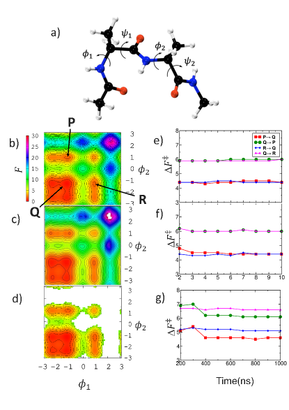
Figure 1: (a) Ball and stick representation of alanine tripeptide (Color codes: H - white, C - black, O - red, and N - blue). Free energy surface $F(\phi_{1},\phi_{2})$ computed using GASS (b), WSMTD (c), and REST2 (d) simulations of alanine tripeptide in water are given. Convergence of free energy barriers for $\mathbf{P}\rightarrow\mathbf{Q}$, $\mathbf{Q}\rightarrow\mathbf{P}$, $\mathbf{R}\rightarrow\mathbf{Q}$, and $\mathbf{Q}\rightarrow\mathbf{R}$ as a function of simulation time in GASS (e), WSMTD (f), and REST2 (g) simulations are shown. Here the angles are in radians and free energies are in kcal mol^-1.

III Results and Discussion

The accuracy and efficiency of the GASS method was first investigated for the exploration of the conformational free energy landscape of alanine tripeptide in explicit water. The performance of the method is compared with REST2 and WSMTD. Thereafter, it was tested for computing the free energy landscape of unfolding of Trp-cage protein in water.

III.1 Alanine Tripeptide in Water

Method	Simulation Time (ns)	$\Delta F^{\ddagger}$				$\Delta F$
		$\mathbf{P}\rightarrow\mathbf{Q}$	$\mathbf{Q}\rightarrow\mathbf{P}$	$\mathbf{R}\rightarrow\mathbf{Q}$	$\mathbf{Q}\rightarrow\mathbf{R}$	$\mathbf{P}-\mathbf{Q}$	$\mathbf{R}-\mathbf{Q}$
GASS	10	4.4	6.0	4.4	6.0	1.6	1.6
WSMTD	10	4.4	6.0	4.4	6.0	1.6	1.6
REST2	1000	4.6	6.1	5.1	6.6	1.5	1.5

Table 1: Free energy barriers ($\Delta F^{\ddagger}$) and free energy differences ($\Delta F$), in kcal mol^-1, computed from the free energy landscape $F(\phi_{1},\phi_{2})$ of alanine tripeptide in water using various methods.

Alanine tripeptide in water was modeled using AMBER14SBff14SB and TIP3PTIP3P force-fields. We took the amino acid sequence ACE-ALA-ALA-NME where the terminal residues ACE and NME were acetyl and N-methyl amide, respectively, and the total number of water molecules in the system is 785. All the bonds in the system were constrained and the equations of motion were integrated using a time step of 1 fs. Long range electrostatics was treated using the particle-mesh Ewald technique, as available in GROMACS.PME Temperature of the system was controlled using the stochastic velocity rescaling thermostat.v-scaling:thermostat Density was converged in 100 ps of $NPT$ simulation and the equilibrated cell volume achieved was $34\times 36\times 30$ Å³. GASS simulations were then carried out in the $NVT$ ensemble using the equilibrated density. In REST2, all the peptide atoms were taken in the hot region and 5 replicas were considered with the values of $\lambda_{m}$ ranging from 1.0 to 0.3 following a geometric distribution. Exchanges between the neighboring replicas were attempted every 1000 MD steps. The two Ramachandran angles $\phi_{1}$ and $\phi_{2}$ were chosen as CVs for biasing; see Figure 1a. Umbrella bias was applied along $\phi_{1}$ from $-\pi$ to $+\pi$ at an interval of 0.2 radians with $\kappa_{h}=1.2\times 10^{2}$ kcal mol^-1 rad^-2 and a well-tempered MTD bias was applied along $\phi_{2}$. The MTD bias was updated every 500 fs, and the bias parameters $w_{0}=0.6$ kcal mol^-1, $\delta s=0.05$ radians, and $\Delta T=900~{}$K were taken. It is noted that the choice of types of biases applied on $\phi_{1}$ and $\phi_{2}$ were arbitrary.

For demonstrating the performance of GASS, we carried out independent WSMTD, and REST2 simulations with identical setups.

Figure  1 shows the free energy surface $F(\phi_{1},\phi_{2})$ computed using GASS, WSMTD, and REST2 and the convergence of free energy barriers for these surfaces. The free energy barriers $\mathbf{Q}\rightarrow\mathbf{P}$ and $\mathbf{Q}\rightarrow\mathbf{R}$ are expected to be nearly the same due to the symmetry, and the same holds true for the corresponding reverse barriers. From Figure 1e, it is clear that very accurate predictions of free energy barriers are possible even after 2 ns of GASS simulation. As anticipated, the $\mathbf{Q}\rightarrow\mathbf{P}$ and $\mathbf{Q}\rightarrow\mathbf{R}$ barriers are found to be equal, and the same is true for $\mathbf{P}\rightarrow\mathbf{Q}$ and $\mathbf{R}\rightarrow\mathbf{Q}$ barriers. A smooth free energy surface was obtained after 10 ns of GASS simulation, and the system swept through the entire two-dimensional landscape.

The free energy barriers computed from independent WSMTD are agreeing very well with the GASS results. Interestingly, the convergence of free energy barriers in their runs was as quick as that using GASS. However, the higher energy regions near $\phi_{1}=2.4$, $\phi_{2}=2.4$ (radians) were not well explored in WSMTD (Figure 1c). The results of independent REST2 simulations (Figure 1d,g) show that conformations far from the free energy minima are not well explored even after 1 $\mu$s and the estimates of the free energy barriers ($\Delta F^{\ddagger}$) are not well converged. On the other hand, free energy differences ($\Delta F$) computed using GASS, WSMTD, and REST2 are agreeing very well; see Table 1.

These results give us the confidence that GASS method is able to provide accurate free energy estimates and could achieve quick conformational sampling. The method is evidently performing better than both WSMTD and REST2 methods.

III.2 Conformational Landscape of Trp-Cage in Water

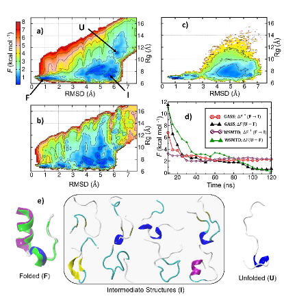
Figure 2: Conformational free energy landscape of Trp-cage protein computed along the RMSD and Rg CVs using (a) GASS (b) WSMTD (c) REST2. (d) Convergence of free energy difference ($\Delta F=F({\mathbf{U}}-{\mathbf{F}})$ ) between the unfolded (U) and the folded state (F) and convergence of free energy barrier for going from F to the intermediate I ($\Delta F^{\ddagger}({\mathbf{F}\rightarrow\mathbf{I}})$) are plotted as function of simulation time. (e) Representative conformations of F, I and U states are shown. The NMR structure (green) is overlapped with F for a comparison. Number of other conformations were also observed in I and U states; See SI Section 4.

As next, we investigated the unfolding/folding landscape of Trp-cage in explicit water using the GASS method. This is an ideal problem to study using GASS as a controlled sampling along a “folding/unfolding coordinate” using the restraining bias could drive the conformations from folded to unfolded states, or vice-versa. At the same time, accelerated sampling of several orthogonal coordinates are essential to boost the exploration of the conformational states for such systems which can be achieved by using MTD bias and REST2.

Trp-cage is a 20 amino acid mini-protein (NLYIQ WLKDG GPSSG RPPPS) designed by Neidigh et al.trp:2002:original from 39 amino acid extendin-4 peptide. It is a fast-folding protein and is considered as an ideal model system for testing computational methods developed for protein-folding problems. It contains a short $\alpha$-helix (residues 2-9), a $3_{10}$-helix (residues 11-14), and a C-terminal polyproline-II helix.

The initial Trp-cage structure for our simulations was built based on the folded NMR structure PDB ID 1L2Y.trp:2002:original The protein was first solvated in a periodic $80\times 80\times 80$ Å³ TIP3P water box with 1 g cm^-3 density. We used AMBER ff14SBff14SB force-field for the protein. Long-range electrostatic interactions were evaluated using the Particle Mesh Ewald method.PME All the bonds in the system were constrained using the LINCS algorithm.LINCS A time step of 2 fs was used to integrate the equation of motion. Temperature of the system was controlled by stochastic velocity rescaling thermostat.v-scaling:thermostat A 1 ns long $NPT$ run was initially carried out using Parrinello-Rahman barostatParrinello:Rehman to obtain converged density and the equilibrated cell volume was found to be $83\times 83\times 83$ Å³. Using the equilibrated system, we performed 10 ns equilibration in $NVT$ ensemble to generate initial structures for the GASS simulation.

All the protein atoms were chosen in the hot region for the REST2 calculations. We chose 20 replicas with $\lambda_{m}$ values ranging from 1.0-0.3 to obtain a good exchange probability. The exchange of coordinates was attempted after every 1000 MD steps.

We chose to apply restraining bias along the backbone root mean square deviation (RMSD) CV in order to drive the unfolding of the protein from the folded starting structure; See SI Section 1.1 for the definition of the coordinate. As the reference structure for computing RMSD, we took the backbone structure of all the heavy atoms for the residues 1 to 15 in the PDB 1L2Y. This CV will serve as the “unfolding coordinate” which will guide the system from folded state to unfolded state in a controlled manner. A total of 45 umbrella windows were placed every 0.20 Å, starting from 0.20 Å. MTD bias was applied along the radius of gyration (Rg) in all the windows; See SI Section 1.2 for the definition of Rg. This bias potential could enhance the conformational sampling by triggering the breakage of $\alpha$-helices, thereby promoting the system to visit unfolded states. Since GASS approach enables us to have different transverse coordinates for different windows, we chose the $\alpha$-helicity (SI Section 1.3) CV together with Rg for applying MTD bias for the windows placed between RMSD values 6.0 Å and 8.0 Å. For the MTD bias, we choose the Gaussian parameters $w_{0}=0.6$ kcal mol^-1, and $\delta s=0.02$. We took $\Delta T=2700$ K and $5700$ K when we used one-dimensional and two-dimensional MTD biases, respectively. We scaled-up the width of the Gaussian by a factor 10 in the direction of the $\alpha-$helicity coordinate because of the large amplitude fluctuation of this CV compared to Rg. The starting umbrella window at RMSD=$0.20$ Å pertained to a folded structure, resembling well with the NMR structure (PDB ID: 1L2Y). Starting structure of all the other windows with higher value of RMSD was taken as the equilibrated structure of the preceding window.

We reconstructed the free energy surface in the RMSD-Rg space after 120 ns of the simualation (Figure 2a). Free energy surfaces constructed after 50 ns, 75 ns, 100 ns of GASS simulation are presented in SI Section 2. The Figure 2a clearly indicates folded $(\mathbf{F})$, semi-unfolded/intermediate $(\mathbf{I})$ and unfolded $(\mathbf{U})$ states of Trp-cage. Representative structures of various conformational minima found on the free surface are obtained by clustering the trajectory of the corresponding GASS window (Figure 2f). They indicate that the conformational space, including the unfolded states, is very well explored. The free energy barrier for $\mathbf{F}\rightarrow\mathbf{I}$, and free energy difference between $\mathbf{F}$ and $\mathbf{U}$ are computed as a function of simulation time (Figure 2d). This plot indicates that the estimate of free energy difference was converged by 100 ns and free energy barrier was converged by 60 ns. After 90 ns, new unfolded states were explored, resulting in a small drift in the convergence curve of $\Delta F$.

Detailed studies on the mechanism of folding have been done experimentallyWountersenJPCB:2013 ; trp:2002:original ; Qiu:2002 ; Ahmed:2005 ; Neuweiler:2005 ; Iavarone:2005 ; Bunagan:2006 ; Streicher:2007 ; Iavarone:2007 ; Mok:2007 ; Hudaky:2008 ; Barua:2008 ; Culik:2011 ; Rovo:2011 ; Ronge:2012 ; Anna:2012 ; Rovo:2013 ; ADAMS:2006 ; Tucker:JPCL:2020 and computationally.WountersenJPCB:2013 ; Vijaypande:2002 ; Adrian:2002 ; CHOWDHURY:2003 ; Zhou:PNAS:2003 ; Bolhuis:PNAS:2006 ; Bolhuis:2008 ; HU:2008 ; Lindorff:2011 ; Shao:2012 ; WU:2011 ; Marino:2012 ; Lai:2013 ; XU:2008 ; Bandyopadhyay:PCCP:2016 ; Ferguson:2018 ; Kim:2016 ; Hatch:2014 ; Kannan:2014 ; Alexander:2005 ; Zhou:Proteins:2003 ; Levy:JPCB:2013 ; Patriksson:2007 ; Pitera:2003 ; trp:2002 ; be:mtd:1 ; be:mtd:2 ; trp:2011 ; trp:2012 ; trp:2013 ; trp:2014 ; trp:2015 ; trp:2015:amd ; trp:2017 ; trp:2018 ; REHT:2021 The protein folding landscape of Trp-cage shows intermediate states, different to the classical picture with only two states. The presence of metastable intermediate states have been seen observed computationally Zhou:PNAS:2003 ; Lindorff:2011 and experimentally.Sauer:PNAS:2005 Two major folding pathways have been identified for this protein.Bolhuis:PNAS:2006 ; Debenedetti:JCP:2015 ; Laio:PLOS:2009 ; Levy:JPCB:2013 The global minimum on the GASS free energy surface (Figure 2a) is located at RMSD$=1.1$ Å, and Rg$=6.8$ Å, and it corresponds to the folded state ($\mathbf{F}$). The same was also observed in independent 120 ns WSMTD (Figure 2b) and 3 $\mu$s REST2 (Figure 2c) simulations. The intermediate ($\mathbf{I}$) and the unfolded ($\mathbf{U}$) states are located on the (RMSD, Rg) free energy surface at ($5.7$ Å, $7.5$ Å), and ($6.2$ Å, $11.0$ Å), respectively. The intermediate state I and the unfolded state U comprised of large number of protein conformations (Figure 2e). The representative structures presented in Figure 2e were obtained by backbone RMSD based clustering of the biased GASS trajectories. We also observed the intermediates SB-I, LOOP-I, and HLX-I reported by Kim et al.Debenedetti:JCP:2015 ; see Supporting Information. However, it is noted that proper characterization of the intermediate states and reaction pathways require analysis of the unbiased GASS trajectories, which was not carried out here. The free energy barrier $\mathbf{F}\rightarrow\mathbf{I}$ is $2.3$ kcal mol^-1 using GASS, while it is $2.4$ kcal mol^-1 and $3.2$ kcal mol^-1 using WSMTD and REST2 simulations, respectively. From the GASS-computed free energy surface, we calculated the barrier for going from F to U state as $3.0$ kcal mol^-1. The I and the U states are only $0.0$ and $0.7$ kcal mol^-1 higher than the F state, respectively. The free energy data and the conformational landscape reported in our study are in excellent qualitative and quantitative agreement with various reports in the literature.trp:2015:amd ; Gracia:2010 Barrier for ${\bf F}\rightarrow{\bf I}$ also agrees with that reported in Refs.REHT:2021 ; Lindorff:2011 The free energy difference between the unfolded and the folded state was experimentally measured as 0.77 kcal mol^-1 at 298K by Streicher and Makhatadze,Makhatadze:BioChem:2007 which is in remarkably good agreement with our estimate ($0.7$ kcal mol^-1).

Although the folded (${\mathbf{F}}$) and intermediate (${\mathbf{I}}$) states were reasonably sampled in WSMTD, the unfolded (${\mathbf{U}}$) states were not (Figure 2b). The computed free energy difference between the $\mathbf{U}$ and ${\mathbf{F}}$ states is not converged in 120 ns of WSMTD (Figure 2d). Sampling of the unfolded states was insufficient even after 3 $\mu$s of REST2; See Figure 2c. The extent of exploration of the RMSD-Rg space is much less in REST2 compared to that in GASS. Further, the free energy surface computed from REST2 trajectory is noisy. Thus we think that REST2 free energy estimates are likely to be not converged. These results underline the importance of the GASS approach.

IV Conclusions

It has been shown that the combination of the global tempering REST2 method with the CV-based biased sampling technique WSMTD, as done in the proposed GASS method, is an efficient way to study conformational sampling and compute free energies of large soft matter systems in solution. A directed conformational sampling achieved by a restrained-bias along a CV, in tandem with an exhaustive sampling of orthogonal coordinates by MTD bias and REST2, makes the GASS method different to other sampling methods. This is a much needed feature for studying various biochemical processes, such as protein folding. Test calculations performed on solvated alanine tripeptide show that the GASS method provides accurate prediction of conformational free energy landscapes. The method has been applied to study the unfolding/folding free energy landscape of Trp-cage protein in water, wherein a controlled unfolding of the protein was accomplished by applying restraining bias along the RMSD coordinate. Orthogonal coordinates were enhanced sampled by REST2, in concert with the explicit MTD bias on Rg and $\alpha$-helicity CVs. A quick convergence in free energy estimates was observed and a good conformational sampling of the unfolded states was noted. The free energy landscape projected on the RMSD-Rg space has three distinct free energy minima corresponding to fully folded, partially unfolded (intermediate), and unfolded states. On the landscape, the free energy barrier to go from folded to the intermediate state is $2.3$ kcal mol^-1 and the folded to the unfolded state is $3.0$ kcal mol^-1. The intermediate and the unfolded states are only $0.0$ and $0.7$ kcal mol^-1 higher than the folded state, respectively. We hope that the new method proposed here will be very useful to study mechanism and free energetics of complex biochemical processes such as protein folding, drug-binding, and diffusion of molecules through membrane. The reweighting codes and the input files for performing GASS simulations reported here are available online.github:gass

Supporting Information

Additional supporting information may be found in the online version of this article.

References

- (1) Karplus, M. and McCammon, J., Sep , (2002), 9, 646–652.
- (2) Lee, E. H.; Hsin, J.; Sotomayor, M.; Comellas, G. and Schulten, K., Structure, 2009, 17(10), 1295–1306.
- (3) Shaw, D. E.; Maragakis, P.; Lindorff-Larsen, K.; Piana, S.; Dror, R. O.; Eastwood, M. P.; Bank, J. A.; Jumper, J. M.; Salmon, J. K.; Shan, Y. and Wriggers, W., Science, 2010, 330(6002), 341–346.
- (4) Dror, R. O.; Dirks, R. M.; Grossman, J.; Xu, H. and Shaw, D. E., Annu. Rev.Biophys., 2012, 41(1), 429–452.
- (5) Chipot, C. and Pohorille, A., Eds., Free Energy Calculations: Theory and Applications in Chemistry and Biology, Springer, Berlin Heidelberg, 2007.
- (6) Vanden-Eijnden, E., J. Comput. Chem., 2009, 30, 1737.
- (7) Tuckerman, M. E., Statistical Mechanics: Theory and Molecular Simulation, Oxford University Press, Oxford, 1st ed., 2010.
- (8) Christ, C. D.; Mark, A. E. and van Gunsteren, W. F., J. Comput. Chem., 2010, 31, 1569–1582.
- (9) Bonella, S.; Meloni, S. and Ciccotti, G., Eur. Phys. J. B, 2012, 85, 97.
- (10) Abrams, C. and Bussi, G., Entropy, 2014, 16(1), 163–199.
- (11) Valsson, O.; Tiwary, P. and Parrinello, M., Annu. Rev. Phys. Chem., 2016, 67, 159.
- (12) Miao, Y. and McCammon, J. A., Mol. Simul., 2016, 42(13), 1046–1055.
- (13) Pietrucci, F., Rev. Phys., 2017, 2, 32–45.
- (14) Peters, B., Reaction Rate Theory and Rare Events, Elsevier, Amsterdam, Netherlands, 2017.
- (15) Awasthi, S. and Nair, N. N., Wiley Interdiscip. Rev. Comput. Mol. Sci., 2019, 9(3), e1398.
- (16) Paul, S.; Nair, N. N. and Harish, V., Mol. Sim., 2019, 45, 1273–1284.
- (17) Scheraga, H. A.; Khalili, M. and Liwo, A., Annu. Rev.Phys. Chem., 2007, 58(1), 57–83.
- (18) Zuckerman, D. M., Annu. Rev. Biophys., 2011, 40(1), 41–62.
- (19) Wingbermühle, S. and Schäfer, L. V., J. Chem. Theory Comput., 2020, 16(7), 4615–4630.
- (20) Acharya, A.; Prajapati, J. D. and Kleinekathöfer, U., J. Chem. Theory Comput., 2021, 17(7), 4564–4577.
- (21) Sugita, Y. and Okamoto, Y., Chem. Phys. Lett., 1999, 314(1), 141–151.
- (22) Liu, P.; Kim, B.; Friesner, R. A. and Berne, B. J., Proc. Natl. Acad. Sci., 2005, 102(39), 13749–13754.
- (23) Wang, L.; Friesner, R. A. and Berne, B. J., J. Phys. Chem. B, 2011, 115(30), 9431–9438.
- (24) Kamiya, M. and Sugita, Y., J. Chem. Phys., 2018, 149(7), 072304.
- (25) Appadurai, R.; Nagesh, J. and Srivastava, A., Nat. Commun., 2021, 12, 958.
- (26) Hamelberg, D.; Mongan, J. and McCammon, J. A., J. Chem. Phys., 2004, 120(24), 11919–11929.
- (27) Grubmüller, H., Sep , (1995), 52, 2893–2906.
- (28) Hamelberg, D.; Mongan, J. and McCammon, J. A., J. Chem. Phys, 2004, 120(24), 11919–11929.
- (29) Lindahl, V.; Lidmar, J. and Hess, B., J. Chem. Phys., 2014, 141(4), 044110.
- (30) Lundborg, M.; Lidmar, J. and Hess, B., J. Chem. Phys., 2021, 154(20), 204103.
- (31) Torrie, G. M. and Valleau, J. P., Chem. Phys. Lett., 1974, 28, 578.
- (32) Torrie, G. and Valleau, J., J. Chem. Phys., 1977, 23, 187–199.
- (33) Laio, A. and Parrinello, M., Proc. Natl. Acad. Sci., 2002, 99(20), 12562–12566.
- (34) Darve, E. and Pohorille, A., J. Chem. Phys., 2001, 115, 9169.
- (35) Morishita, T.; Itoh, S. G.; Okumura, H. and Mikami, M., Jun , (2012), 85, 066702.
- (36) Morishita, T.; Itoh, S. G.; Okumura, H. and Mikami, M., Jun , (2012), 85, 066702.
- (37) Abrams, J. B. and Tuckerman, M. E., J. Phys. Chem. B, 2008, 112(49), 15742–15757.
- (38) Valsson, O. and Parrinello, M., Phys. Rev. Lett., 2014, 113, 090601.
- (39) Barducci, A.; Bussi, G. and Parrinello, M., Jan , (2008), 100, 020603.
- (40) Piana, S. and Laio, A., J. Phys. Chem. B, 2007, 111, 4553.
- (41) Pfaendtner, J. and Bonomi, M., J. Chem. Theory Comput., 2015, 11(11), 5062–5067.
- (42) Awasthi, S.; Kapil, V. and Nair, N. N., J. Comput. Chem., 2016, 37, 1413.
- (43) Noé, F. and Clementi, C., Curr. Oppin. Struct. Biol., 2017, 43, 141–147.
- (44) Clementi, C. and Henkelman, G., J. Chem. Phys., 2017, 147(15), 152401.
- (45) Husic, B. E. and Pande, V. S., J. Am. Chem. Soc., 2018, 140(7), 2386–2396.
- (46) Sittel, F. and Stock, G., J. Chem. Phys., 2018, 149(15), 150901.
- (47) Chen, M.; Cuendet, M. A. and Tuckerman, M. E., J. Chem. Phys., 2012, 137(2), 024102.
- (48) Awasthi, S. and Nair, N. N., J. Chem. Phys., 2017, 146, 094108.
- (49) Kokubo, H.; Tanaka, T. and Okamoto, Y., J. Chem. Theory Comput., 2013, 9(10), 4660–4671.
- (50) Gil-Ley, A. and Bussi, G., J. Chem. Theory Comput., 2015, 11(3), 1077–1085.
- (51) Bussi, G.; Gervasio, F. L.; Laio, A. and Parrinello, M., J. Am. Chem. Soc., 2006, 128(41), 13435–13441.
- (52) Kokubo, H.; Tanaka, T. and Okamoto, Y., J. Comput. Chem., 2013, 34(30), 2601–2614.
- (53) Galvelis, R. and Sugita, Y., J. Comput. Chem., 2015, 36(19), 1446–1455.
- (54) Yamamori, Y. and Kitao, A., J. Chem. Phys., 2013, 139(14), 145105.
- (55) Camilloni, C. and Pietrucci, F., Adv. Phys., 2018, 3(1), 1477531.
- (56) Meißner, R. H.; Wei, G. and Ciacchi, L. C., Soft Matter, 2015, 11, 6254–6265.
- (57) Kannan, S. and Zacharias, M., Proteins: Struct., Funct., Bioinfo., 2007, 66(3), 697–706.
- (58) Mori, T.; Miyashita, N.; Im, W.; Feig, M. and Sugita, Y., Biochim. Biophys. Acta. Biomembr., 2016, 1858(7, Part B), 1635–1651.
- (59) Rick, S. W.; Schwing, G. J. and Summa, C. M., J. Chem. Inf. Model., 2021, 61(2), 810–818.
- (60) Das, C. K. and Nair, N. N., Phys. Chem. Chem. Phys., 2017, 19, 13111–13121.
- (61) Das, C. K. and Nair, N. N., Phys. Chem. Chem. Phys., 2018, 20, 14482–14490.
- (62) Mandal, S.; Debnath, J.; Meyer, B. and Nair, N. N., J. Chem. Phys., 2018, 149(14), 144113.
- (63) Das, C. K. and Nair, N. N., Chem. Eur. J., 2020, 26(43), 9639–9651.
- (64) Mandal, S. and Nair, N. N., J. Comput. Chem., 2020, 41(19), 1790–1797.
- (65) Mandal, S.; Thakkur, V. and Nair, N. N., J. Chem. Theory Comput., 2021, 17(4), 2244–2255.
- (66) Tiwary, P. and Parrinello, M., J. Phys. Chem. B, 2015, 119(3), 736–742.
- (67) Ferrenberg, A. M. and Swendsen, R. H., Phys. Rev. Lett., 1989, 63, 1195.
- (68) Kumar, S.; Rosenberg, J. M.; Bouzida, D.; Swendsen, R. H. and Kollman, P. A., J. Comput. Chem., 1992, 13, 1011.
- (69) Juraszek, J. and Bolhuis, P. G., Biophys J., 2010, 98, 646–656.
- (70) Berendsen, H.; van der Spoel, D. and van Drunen, R., Comput. Phys. Commun., 1995, 91(1), 43 – 56.
- (71) Tribello, G. A.; Bonomi, M.; Branduardi, D.; Camilloni, C. and Bussi, G., Comput. Phys. Commun., 2014, 185(2), 604–613.
- (72) Bonomi, M.; Branduardi, D.; Bussi, G.; Camilloni, C.; Provasi, D.; Raiteri, P.; Donadio, D.; Marinelli, F.; Pietrucci, F.; Broaglia, R. A. and Parrinello, M., Comput. Phys. Commun., 2009, 180, 1961.
- (73) Bussi, G., Mol. Phys., 2014, 112(3-4), 379–384.
- (74) Maier, J. A.; Martinez, C.; Kasavajhala, K.; Wickstrom, L.; Hauser, K. E. and Simmerling, C., J. Chem. Theory Comput., 2015, 11, 3696.
- (75) MacKerell, A. D.; Bashford, D.; Bellott, M.; Dunbrack, R. L.; Evanseck, J. D.; Field, M. J.; Fischer, S.; Gao, J.; Guo, H.; Ha, S.; Joseph-McCarthy, D.; Kuchnir, L.; Kuczera, K.; Lau, F. T. K.; Mattos, C.; Michnick, S.; Ngo, T.; Nguyen, D. T.; Prodhom, B.; Reiher, W. E.; Roux, B.; Schlenkrich, M.; Smith, J. C.; Stote, R.; Straub, J.; Watanabe, M.; Wiórkiewicz-Kuczera, J.; Yin, D. and Karplus, M., J. Phys. Chem. B, 1998, 102(18), 3586–3616.
- (76) Essmann, U.; Perera, L.; Berkowitz, M. L.; Darden, T.; Lee, H. and Pedersen, L. G., J. Chem. Phys., 1995, 103(19), 8577–8593.
- (77) Bussi, G.; Zykova-Timan, T. and Parrinello, M., J. Chem. Phys., 2009, 130(7), 074101.
- (78) Neidigh, J.; Fesinmeyer, R. and Andersen, N., Nat. Struct. Biol., 2002, 9, 425–430.
- (79) Hess, B.; Bekker, H.; Berendsen, H. J. C. and Fraaije, J. G. E. M., J. Comput. Chem., 1997, 18(12), 1463–1472.
- (80) Parrinello, M. and Rahman, A., J. Appl. Phys., 1981, 52(12), 7182–7190.
- (81) Meuzelaar, H.; Marino, K. A.; Huerta-Viga, A.; Panman, M. R.; Smeenk, L. E. J.; Kettelarij, A. J.; van Maarseveen, J. H.; Timmerman, P.; Bolhuis, P. G. and Woutersen, S., J. Phys. Chem. B, 2013, 117(39), 11490–11501.
- (82) Qiu, L.; Pabit, S. A.; Roitberg, A. E. and Hagen, S. J., J. Am. Chem. Soc., 2002, 124(44), 12952–12953.
- (83) Ahmed, Z.; Beta, I. A.; Mikhonin, A. V. and Asher, S. A., J. Am. Chem. Soc., 2005, 127(31), 10943–10950.
- (84) Neuweiler, H.; Doose, S. and Sauer, M., Proc. Natl. Acad. Sci., 2005, 102(46), 16650–16655.
- (85) Iavarone, A. T. and Parks, J. H., J. Am. Chem. Soc., 2005, 127(24), 8606–8607.
- (86) Bunagan, M. R.; Yang, X.; Saven, J. G. and Gai, F., J. Phys. Chem. B, 2006, 110(8), 3759–3763.
- (87) Streicher, W. W. and Makhatadze, G. I., Biochem., 2007, 46(10), 2876–2880.
- (88) Iavarone, A. T.; Patriksson, A.; van der Spoel, D. and Parks, J. H., J. Am. Chem. Soc., 2007, 129(21), 6726–6735.
- (89) Mok, K. H.; Kuhn, L. T.; Goez, M.; Day, I. J.; Lin, J. C.; Andersen, N. H. and Hore, P. J., Nat., 2007, 447(7140), 106–109.
- (90) Hudáky, P.; Stráner, P.; Farkas, V.; Váradi, G.; Tóth, G. and Perczel, A., Biochem. , 2008, 47(3), 1007–1016.
- (91) Barua, B.; Lin, J. C.; Williams, V. D.; Kummler, P.; Neidigh, J. W. and Andersen, N. H., mar , (2008), 21(3), 171–185.
- (92) Culik, R. M.; Serrano, A. L.; Bunagan, M. R. and Gai, F., Angew. Chem. Int. Ed. , 2011, 50(46), 10884–10887.
- (93) Rovó, P.; Farkas, V.; Hegyi, O.; Szolomájer-Csikós, O.; Tóth, G. K. and Perczel, A., J. Pep. Sci. , 2011, 17(9), 610–619.
- (94) Rogne, P.; Ozdowy, P.; Richter, C.; Saxena, K.; Schwalbe, H. and Kuhn, L. T., 07 , (2012), 7(7), 1–13.
- (95) Hałabis, A.; Żmudzińska, W.; Liwo, A. and Ołdziej, S., J. Phys. Chem. B, 2012, 116(23), 6898–6907.
- (96) Rovó, P.; Stráner, P.; Láng, A.; Bartha, I.; Huszár, K.; Nyitray, L. and Perczel, A., Chem. Euro. J., 2013, 19(8), 2628–2640.
- (97) Adams, C. M.; Kjeldsen, F.; Patriksson, A.; van der Spoel, D.; Gräslund, A.; Papadopoulos, E. and Zubarev, R. A., Int. J. Mass Spectrom. , 2006, 253(3), 263–273.
- (98) Chalyavi, F.; Schmitz, A. J. and Tucker, M. J., J. Phys. Chem. Lett., 2020, 11(3), 832–837.
- (99) Snow, C. D.; Zagrovic, B. and Pande, V. S., J. Am. Chem. Soc., 2002, 124(49), 14548–14549.
- (100) Simmerling, C.; Strockbine, B. and Roitberg, A. E., J. Am. Chem. Soc., 2002, 124(38), 11258–11259.
- (101) Chowdhury, S.; Lee, M. C.; Xiong, G. and Duan, Y., J. Mol. Biol. , 2003, 327(3), 711–717.
- (102) Zhou, R., Proc. Natl. Acad. Sci., 2003, 100(23), 13280–13285.
- (103) Juraszek, J. and Bolhuis, P. G., Proc. Natl. Acad. Sci., 2006, 103(43), 15859–15864.
- (104) Juraszek, J. and Bolhuis, P. G., Biophys. J. , 2008, 95(9), 4246–4257.
- (105) Hu, Z.; Tang, Y.; Wang, H.; Zhang, X. and Lei, M., Arch. Biochem. Biophys. , 2008, 475(2), 140–147.
- (106) Lindorff-Larsen, K.; Piana, S.; Dror, R. O. and Shaw, D. E., Science, 2011, 334(6055), 517–520.
- (107) Shao, Q.; Shi, J. and Zhu, W., J. Chem. Phys., 2012, 137(12), 125103.
- (108) Wu, X.; Yang, G.; Zu, Y.; Fu, Y.; Zhou, L. and Yuan, X., Comp. Theoretical Chem., 2011, 973(1), 1–8.
- (109) Marino, K. A. and Bolhuis, P. G., J. Phys. Chem. B, 2012, 116(39), 11872–11880.
- (110) Lai, Z.; Preketes, N. K.; Mukamel, S. and Wang, J., J. Phys. Chem. B, 2013, 117(16), 4661–4669.
- (111) Xu, W. and Mu, Y., Biophys. Chem., 2008, 137(2), 116–125.
- (112) Gupta, M.; Nayar, D.; Chakravarty, C. and Bandyopadhyay, S., Phys. Chem. Chem. Phys., 2016, 18, 32796–32813.
- (113) Chen, W. and Ferguson, A. L., J. Comput. Chem., 2018, 39(25), 2079–2102.
- (114) Kim, S. B.; Gupta, D. R. and Debenedetti, P. G., Sci. Rep. , 2016, 6(1), 25612.
- (115) Hatch, H. W.; Stillinger, F. H. and Debenedetti, P. G., J. Phys. Chem. B, 2014, 118(28), 7761–7769.
- (116) Kannan, S. and Zacharias, M., 02 , (2014), 9, 1–12.
- (117) Schug, A.; Wenzel, W. and Hansmann, U. H. E., J. Chem. Phys., 2005, 122(19), 194711.
- (118) Zhou, R., Proteins: Struct., Funct., Bioinfo., 2003, 53(2), 148–161.
- (119) Deng, N.-j.; Dai, W. and Levy, R. M., J. Phys. Chem. B, 2013, 117(42), 12787–12799.
- (120) Patriksson, A.; Adams, C. M.; Kjeldsen, F.; Zubarev, R. A. and van der Spoel, D., J. Phys. Chem. B, 2007, 111(46), 13147–13150.
- (121) Pitera, J. W. and Swope, W., Proc. Natl. Acad. Sci., 2003, 100(13), 7587–7592.
- (122) Qiu, L.; Pabit, S. A.; Roitberg, A. E. and Hagen, S. J., J. Am. Chem. Soc., 2002, 124(44), 12952–12953.
- (123) Marinelli, F.; Pietrucci, F.; Laio, A. and Piana, S., PLoS Comput. Biol., 2009, 5, e1000452.
- (124) Paschek, D.; Day, R. and García, A. E., Phys. Chem. Chem. Phys., 2011, 13, 19840–19847.
- (125) Wu, X.; Yang, G.; Zu, Y.; Fu, Y.; Zhou, L. and Yuan, X., Mol. Simul., 2012, 38(2), 161–171.
- (126) Lee, I.-H. and Kim, S.-Y., BioMed. Res. Int., 2013, pages 2314–6133.
- (127) Byrne, A.; Williams, D. V.; Barua, B.; Hagen, S. J.; Kier, B. L. and Andersen, N. H., Biochemistry, 2014, 53(38), 6011–6021.
- (128) Bille, A.; Linse, B.; Mohanty, S. and Irbäck, A., J. Chem. Phys., 2015, 143(17), 175102.
- (129) Miao, Y.; Feixas, F.; Eun, C. and McCammon, J. A., J. Comput. Chem., 2015, 36(20), 1536–1549.
- (130) Meshkin, H. and Zhu, F., J. Chem. Theory Comput., 2017, 13(5), 2086–2097.
- (131) Kamiya, M. and Sugita, Y., J. Chem. Phys., 2018, 149(7), 072304.
- (132) Neuweiler, H.; Doose, S. and Sauer, M., Proc. Natl. Acad. Sci., 2005, 102(46), 16650–16655.
- (133) Kim, S. B.; Dsilva, C. J.; Kevrekidis, I. G. and Debenedetti, P. G., J. Chem. Phys., 2015, 142(8), 085101.
- (134) Marinelli, F.; Pietrucci, F.; Laio, A. and Piana, S., 08 , (2009), 5(8), 1–18.
- (135) Day, R.; Paschek, D. and Garcia, A. E., Proteins: Struct., Funct., Bioinfo., 2010, 78(8), 1889–1899.
- (136) Streicher, W. W. and Makhatadze, G. I., Biochem., 2007, 46(10), 2876–2880.
- (137) Input files and reconstruction codes for gass simulation https://github.com/anjibabuIITK/GASS.