First deep images catalogue of extended IPHAS PNe

L. Sabin

{}^{1\href https://orcid.org/0000-0003-0242-0044{}}

, M.A. Guerrero

{}^{2\href https://orcid.org/0000-0002-7759-106X{}}

, G. Ramos-Larios

{}^{3\href https://orcid.org/0000-0003-2653-4417{}}

, P. Boumis

{}^{4\href https://orcid.org/0000-0002-4260-940X{}}

, A. A. Zijlstra

{}^{5,6\href https://orcid.org/0000-0002-3171-5469{}}

, D. N. F. Awang Iskandar

{}^{7\href https://orcid.org/0000-0002-0909-5670{}}

, M. J. Barlow

{}^{8\href https://orcid.org/0000-0002-3875-1171{}}

, J. A. Toalá

{}^{9\href https://orcid.org/0000-0002-5406-0813{}}

, Q. A. Parker

{}^{10\href https://orcid.org/0000-0002-2062-0173{}}

, R. M. L. Corradi

{}^{11,12\href https://orcid.org/0000-0002-7865-6056{}}

and R. A. H. Morris¹³
¹Instituto de Astronomía, Universidad Nacional Autónoma de México, Apdo. Postal 106, 22800 Ensenada, B.C., Mexico
²Instituto de Astrofísica de Andalucía (IAA-CSIC), Glorieta de la Astronomía S/N, 18008 Granada, Spain
³Instituto de Astronomía y Meteorología, CUCEI, Universidad de Guadalajara, Av. Vallarta 2602, Arcos Vallarta, 44130 Guadalajara, Mexico
⁴Institute for Astronomy, Astrophysics, Space Applications and Remote Sensing, National Observatory of Athens, 15236 Penteli, Athens, Greece
⁵Jodrell Bank Centre for Astrophysics, The University of Manchester, Oxford Road, Manchester M13 9PL, UK
⁶Laboratory for Space Research, University of Hong Kong, Pokfulam Road, Hong Kong
⁷Faculty of Computer Science and Information Technology, Universiti Malaysia Sarawak, Sarawak 94300, Malaysia
⁸Dept. of Physics & Astronomy, University College London, Gower St, London WC1E 6BT,UK
⁹Instituto de Radioastronomía y Astrofísica, UNAM, Campus Morelia, C.P. 58089, Morelia, Mexico
¹⁰Department of Physics, The University of Hong Kong, Chong Yuet Ming Physics Building Pokfulam Road, Hong Kong
¹¹GRANTECAN, Cuesta de San José s/n, E-38712, Breña Baja, La Palma, Spain
¹²Instituto de Astrofísica de Canarias, E-38200 La Laguna, Tenerife, Spain
¹³School of Physics, Bristol University, Tyndall Avenue, Bristol, BS8 1TL, UK E-mail:lsabin@astro.unam.mx (LS)

Abstract

We present the first instalment of a deep imaging catalogue containing 58 True, Likely and Possible extended PNe detected with the Isaac Newton Telescope Photometric H $\alpha$ Survey (IPHAS). The three narrow-band filters in the emission lines of H $\alpha$ , [N ii] $\lambda$ 6584 Å, and [O iii] $\lambda$ 5007 Å used for this purpose allowed us to improve our description of the morphology and dimensions of the nebulae. In some cases even the nature of the source has been reassessed. We were then able to unveil new macro- and micro-structures, which will without a doubt contribute to a more accurate analysis of these PNe. It has been also possible to perform a primary classification of the targets based on their ionization level. A Deep Learning classification tool has also been tested. We expect that all the PNe from the IPHAS catalogue of new extended planetary nebulae will ultimately be part of this deep H $\alpha$ , [N ii] and [O iii] imaging catalogue.

keywords:

stars: winds and outflows — stars: mass-loss — (ISM:) planetary nebulae

^†^†pubyear: 2021^†^†pagerange: First deep images catalogue of extended IPHAS PNe–LABEL:lastpage

1 Introduction

Table 1: Observational setup

Setup	Date	Telescope	Instrument	CCD	Plate scale	FoV	Filter 1	Filter 2	Filter 3	Exposure Time
					(arcsec)	(arcmin)				(s)
N1	2007-09	NOT	ALFOSC	E2V 42-40 2k $\times$ 2k	0.189	6.5	[O iii] #40 NOT	H $\alpha$ #21 NOT	[N ii] #78 NOT	1 $\times$ 1200
N2	2015-07	NOT	ALFOSC	E2V 42-40 2k $\times$ 2k	0.189	6.5	[O iii] #40 NOT	H $\alpha$ #21 NOT	[N ii] #78 NOT	3 $\times$ 450
N3	2015-09	NOT	ALFOSC	E2V 42-40 2k $\times$ 2k	0.189	6.5	[O iii] #90 NOT	H $\alpha$ #21 NOT	[N ii] #78 NOT	3 $\times$ 600
N4	2016-05	NOT	ALFOSC	E2V CCD231-42 2k $\times$ 2k	0.211	7.1	[O iii] #90 NOT	H $\alpha$ #21 NOT	[N ii] #78 NOT	3 $\times$ 600
N4	2016-11	NOT	ALFOSC	E2V CCD231-42 2k $\times$ 2k	0.211	7.1	[O iii] #90 NOT	H $\alpha$ #21 NOT	[N ii] #78 NOT	3 $\times$ 600
N5	2018-06	NOT	ALFOSC	E2V CCD231-42 2k $\times$ 2k	0.211	7.1	[O iii] #90 NOT	H $\alpha$ OSN	[N ii] OSN	3 $\times$ 600
N5	2018-09	NOT	ALFOSC	E2V CCD231-42 2k $\times$ 2k	0.211	7.1	[O iii] #90 NOT	H $\alpha$ OSN	[N ii] OSN	3 $\times$ 600
N5	2020-01	NOT	ALFOSC	E2V CCD231-42 2k $\times$ 2k	0.211	7.1	[O iii] #90 NOT	H $\alpha$ OSN	[N ii] OSN	3 $\times$ 600
A1	2016-11	AT	LN2CCD	E2V CCD42-40 2k $\times$ 2k	0.16	5.5	[O iii] AT	H $\alpha$ AT	[N ii] AT	3 $\times$ 800
A2	2016-08	AT	LN2CCD	E2V CCD42-40 2k $\times$ 2k	0.16	5.5	[O iii] AT	H $\alpha$ AT	[N ii] AT	1 $\times$ 1200
A2	2016-09	AT	LN2CCD	E2V CCD42-40 2k $\times$ 2k	0.16	5.5	[O iii] AT	H $\alpha$ AT	[N ii] AT	1 $\times$ 1200
A1	2017-08	AT	LN2CCD	E2V CCD42-40 2k $\times$ 2k	0.16	5.5	[O iii] AT	H $\alpha$ AT	[N ii] AT	3 $\times$ 800
A1	2017-10	AT	LN2CCD	E2V CCD42-40 2k $\times$ 2k	0.16	5.5	[O iii] AT	H $\alpha$ AT	[N ii] AT	3 $\times$ 800
A1	2018-06	AT	LN2CCD	E2V CCD42-40 2k $\times$ 2k	0.16	5.5	[O iii] AT	H $\alpha$ AT	[N ii] AT	3 $\times$ 800

The Isaac Newton Telescope Photometric H $\alpha$ Survey of the Northern Galactic Plane (IPHAS; Drew, et al. 2005) has allowed the detection of a significant number of new planetary nebulae (PNe) candidates. More than 150 of those have already been confirmed in follow-up spectroscopic observations (Sabin, et al. 2014) and more are will be presented in upcoming papers (Ritter et al., in preparation).

The observational strategy of IPHAS was optimized to guaranty the completion of the survey in a reasonable amount of time with the acquisition of images in the Sloan $i^{\prime}$ and $r^{\prime}$ filters and through a 95 Å wide H $\alpha$ filter with fixed exposure times of 10 s, 30 s and 120 s, respectively¹¹1 We note that a database of images from the INT Galactic Plane Survey (IGAPS, Monguió et al. 2020) will soon be published (Greimel et al. submitted).. The shallow IPHAS images thus provided only limited information on the morphologies of those new PNe. Furthermore, IPHAS does not provide information on the ionization structure because the used filter includes both the H $\alpha$ and [N ii] $\lambda$ 6583Å emission lines. The PN morphology, however, depends strongly on the excitation of the ion emitting a particular line. In particular, the [O iii] $\lambda$ 5007Å emission line preferentially reveals the morphology of high-excitation nebular regions, whereas the [N ii] $\lambda$ 6584 Å emission line reveals low-excitation regions and features (see for example the catalogues by Manchado et al. 1996 and Stanghellini, Shaw, & Villaver 2016).

It is thus very likely that the faintest nebular structures and low-excitation features such as outflows/jets or knots can still elude us in IPHAS images. Not only the detailed morphology of the IPHAS PNe is compromised, but also their exact sizes might require a deeper and sharper imaging. This information can be expected to give us more insights into the formation process and more generally the characteristics of these PNe. Therefore we focus on the morphological and nebular excitation analysis in this new instalment on our study of IPHAS PNe presenting a multi-wavelength optical H $\alpha$ , [N ii] and [O iii] imaging survey of 58 True, Likely and Possible extended planetary nebulae selected mainly from the IPHAS Catalogue of New Extended Planetary Nebulae (Sabin, et al. 2014, hereafter Paper I), but also from the follow-up spectroscopy program (Ritter et al., in prep). The article is organized as follows. The observations are presented in section §2, the list of objects and images are described in section §3, and our discussion in section §4. The conclusions are presented in section §5.

Table 2: Properties of the narrow-band filters

Telescope	Filter	Central Wavelength	FWHM	Transmission
		(Å)	(Å)	(%)
AT	H $\alpha$ 6563 Å	6567	17.0	69.6
AT	[O iii] 5007 Å	5011	30.0	83.9
AT	[N ii] 6583 Å	6568	17.0	79.6
OSN	H01 H $\alpha$	6564.6	12.7	80.2
OSN	E16 [N ii]	6583.3	12.6	79.2
NOT	H $\alpha$ #21	6564	3.3	66.0
NOT	[O iii] #40	5010	4.3	56.0
NOT	[N ii] #78	6583	3.6	74.0

2 NOT and Helmos Observations

We have acquired narrow-band images in the [O iii] $\lambda$ 5007 Å, H $\alpha$ , and [N ii] $\lambda$ 6584 Å emission lines using the ALhambra Faint Object Spectrograph and Camera (ALFOSC) installed on the 2.56-m Nordic Optical Telescope (NOT) at the Observatorio de El Roque de los Muchachos (ORM) in La Palma (Spain) and the LN2CCD imaging camera at the 2.3-m (f/8) Aristarchos telescope (AT) of Helmos Observatory in Peloponese (Greece). The instrumental setup has been changing between the different observational runs and we summarize the information regarding the detectors, plate scale, field-of-view (FoV), filters and number of frames and integration time of individual exposures in Table 1 and Table 2. A code is assigned to each instrumental setup in the first column of Table 1.

All the data were bias-subtracted and then flat-fielded using twilight flats employing standard iraf (Tody 1993) routines²²2iraf, the Image Reduction and Analysis Facility, is distributed by the National Optical Astronomy Observatory, which is operated by the Association of Universities for Research in Astronomy (AURA) under cooperative agreement with the National Science Foundation..

3 Results

The complete list of objects studied here is presented in Table 3 and their individual H $\alpha$ , [N ii] and [O iii] narrow-band images in addition to colour-composite are presented in Figures 4–15 of Appendix A. For simplicity, each object listed in Table 3 is identified by its identification number as defined in Paper I (and other papers of this series), therefore adopting the Sab # denomination hereafter³³3But the last source in Table 3, named J191104.8, which is not listed in Paper I., as well as by the standard and official IAU PNG and IPHAS identifications. For each object we list next the code describing the instrumental setup used (as defined in the first column of Table 1), the observing date and the average seeing during the observation. In the following section, we present the main characteristics and features that can be derived from the deep images.

It is important to emphasize that the main goal of the observing program presented here is the acquisition of morphological information on different emission lines for IPHAS PNe. Therefore the observing program did not include standard stars for flux calibration (and surface brightness measurement). A proper calibration of the images taking into account the characteristics of the different filters and guided by spectroscopic data for some of the sources in our sample will be presented in a forthcoming paper.

4 Discussion

Table 3: IPHAS sources observed with the Nordic Optical Telescope (NOT) and Aristarchos telescope (AT, Helmos Observatory). Sab numbers, designation, coordinates and the observation date are listed. Notes: The asterisks "*" indicate a change in total size (from the originally reported dimensions)

\geq 10\arcsec

\dagger

the full size is taken from Mampaso et al. 2006. Note that Sab 15 and 50 are now rejected as PNe.

Sab #	IAU PNG	IPHAS ID:	Setup	Obs. date	Seeing	Major Diam.	Morphology
	designation	IPHASX		yyyy-mm-dd	(arcsec)	(arcsec)	Old $\rightarrow$ New
2	G119.2 $+$ 04.6	J001333.8 $+$ 671803	N4	2016-11-28	0 $\aas@@fstack{\prime\prime}$ 8	^∗46	B $\rightarrow$ Bprs
4	G126.6 $+$ 01.3	J012507.9 $+$ 635652^a	N3	2015-10-02	0 $\aas@@fstack{\prime\prime}$ 7	$\dagger$ 105	Bamp $\rightarrow$ Bampr
6	G129.6 $+$ 03.4	J015624.9 $+$ 652830	A1	2016-11-05	1 $\aas@@fstack{\prime\prime}$ 0	196	Rar $\rightarrow$ Rms
7	G132.8 $+$ 02.0	J022045.0 $+$ 631134	N3	2015-10-02	0 $\aas@@fstack{\prime\prime}$ 6	33	Eas $\rightarrow$ Es
11	G144.1 $-$ 00.5	J033105.3 $+$ 553851	N4	2016-11-27	0 $\aas@@fstack{\prime\prime}$ 7	^∗36	Rar $\rightarrow$ Ras
13	G150.0 $-$ 00.3	J040329.5 $+$ 520825	N5	2020-01-26	0 $\aas@@fstack{\prime\prime}$ 8–1 $\aas@@fstack{\prime\prime}$ 3	^∗34	Bp $\rightarrow$ Bp
15	G159.4 $+$ 02.0	J045358.6 $+$ 465842	N5	2020-01-26	1 $\aas@@fstack{\prime\prime}$ 0	^∗126	Am $\rightarrow$ I
19	G183.0 $+$ 00.0	J055242.8 $+$ 262116^b	N5	2020-01-26	1 $\aas@@fstack{\prime\prime}$ 0	16	Rar $\rightarrow$ Ram
21	G190.7 $-$ 01.3	J060412.2 $+$ 190031	N5	2020-01-26	1 $\aas@@fstack{\prime\prime}$ 1	72	Ba $\rightarrow$ Bp
22	G195.4 $-$ 04.0	J060416.2 $+$ 133250	N4	2016-11-28	1 $\aas@@fstack{\prime\prime}$ 1	^∗75	Ba $\rightarrow$ Br
23	G204.3 $-$ 01.6	J062937.8 $+$ 065220	N4	2016-11-28	0 $\aas@@fstack{\prime\prime}$ 8	31	Ba $\rightarrow$ Br
31	G038.4 $+$ 03.6	J184834.6 $+$ 063302	A2	2016-08-05	2 $\aas@@fstack{\prime\prime}$ 0	25	Ba $\rightarrow$ A/Ba
36	G032.7 $-$ 00.5	J185312.9 $-$ 002529	A2	2016-08-05	1 $\aas@@fstack{\prime\prime}$ 6	26	E $\rightarrow$ E
39	G032.9 $-$ 01.4	J185640.0 $-$ 003804	A2	2016-08-06	1 $\aas@@fstack{\prime\prime}$ 6	21	Bp $\rightarrow$ Br
40	G043.3 $+$ 03.5	J185744.4 $+$ 105053	A2	2016-08-05	1 $\aas@@fstack{\prime\prime}$ 9	110	Eams $\rightarrow$ Eas
42	G040.6 $+$ 01.5	J185957.0 $+$ 073544	N5	2018-06-05	0 $\aas@@fstack{\prime\prime}$ 8–1 $\aas@@fstack{\prime\prime}$ 1	5	B $\rightarrow$ B/S
44	G044.4 $+$ 03.1	J190115.5 $+$ 114150	A2	2016-08-06	1 $\aas@@fstack{\prime\prime}$ 5	30	Ear $\rightarrow$ Ra
50	G038.7 $-$ 00.5	J190401.5 $+$ 045433	N2	2015-07-17	0 $\aas@@fstack{\prime\prime}$ 6	>140	Ims $\rightarrow$ I
53	G036.4 $-$ 01.9	J190438.6 $+$ 021424	N4	2016-05-02	0 $\aas@@fstack{\prime\prime}$ 8	21	Bmp $\rightarrow$ Bmpw
54	G045.4 $+$ 02.6	J190447.9 $+$ 121844	N5	2018-09-08	0 $\aas@@fstack{\prime\prime}$ 7	12	Er $\rightarrow$ Br
55	G043.6 $+$ 01.7	J190454.0 $+$ 101801	A2	2016-08-06	1 $\aas@@fstack{\prime\prime}$ 6	20	Ears $\rightarrow$ Ra
61	G038.9 $-$ 01.3	J190718.1 $+$ 044056	N4	2016-05-01	0 $\aas@@fstack{\prime\prime}$ 9	12	I $\rightarrow$ Bmpsw
63	G045.7 $+$ 01.4	J190954.7 $+$ 120455	N4	2016-05-01	1 $\aas@@fstack{\prime\prime}$ 1	18	B $\rightarrow$ Es
65	G044.9 $+$ 00.8	J191022.1 $+$ 110538	N5	2018-06-07	1 $\aas@@fstack{\prime\prime}$ 0	11	Ear $\rightarrow$ Ems
69	G047.6 $+$ 01.0	J191445.1 $+$ 133219	N4	2016-05-01	1 $\aas@@fstack{\prime\prime}$ 5	16	Ears $\rightarrow$ Em
79	G051.7 $+$ 01.3	J192146.7 $+$ 172055	N2	2015-07-19	1 $\aas@@fstack{\prime\prime}$ 5–1 $\aas@@fstack{\prime\prime}$ 8	34	Ears $\rightarrow$ Ia
81	G049.2 $+$ 00.0	J192153.9 $+$ 143056	N5	2018-09-09	0 $\aas@@fstack{\prime\prime}$ 9	^∗60	Ear $\rightarrow$ Br
86	G049.5 $-$ 01.4	J192751.3 $+$ 140127	N5	2018-09-10	0 $\aas@@fstack{\prime\prime}$ 9	14	Rars $\rightarrow$ Ia
88	G045.7 $-$ 03.8	J192847.2 $+$ 093436	N2	2015-07-18	0 $\aas@@fstack{\prime\prime}$ 7	72	Br $\rightarrow$ Brs
99	G056.1 $-$ 00.4	J193718.6 $+$ 202102^c	N4	2016-11-27	0 $\aas@@fstack{\prime\prime}$ 9	^∗64	Bas $\rightarrow$ Brs
105	G063.3 $+$ 02.2	J194240.5 $+$ 275109	A1	2017-08-20	2 $\aas@@fstack{\prime\prime}$ 4	76	Rar $\rightarrow$ Ra
106	G054.2 $-$ 03.4	J194359.5 $+$ 170901^d	N1	2007-09-03	0 $\aas@@fstack{\prime\prime}$ 7	^∗120	Bamps $\rightarrow$ Bmprs
108	G057.8 $-$ 01.7	J194533.6 $+$ 210808	A1	2016-11-05	1 $\aas@@fstack{\prime\prime}$ 8	^∗118	Ear $\rightarrow$ Is
109	G059.8 $-$ 00.6	J194556.2 $+$ 232833	A1	2018-06-06	1 $\aas@@fstack{\prime\prime}$ 0	58	Bas $\rightarrow$ Es
111	G059.7 $-$ 01.0	J194727.5 $+$ 230816	N2	2015-07-19	1 $\aas@@fstack{\prime\prime}$ 3	40	Rars $\rightarrow$ Rs
113	G066.8 $+$ 02.9	J194751.9 $+$ 311818	N5	2018-09-08	0 $\aas@@fstack{\prime\prime}$ 8	13	B $\rightarrow$ Bpw
116	G062.7 $+$ 00.0	J194940.9 $+$ 261521	N1	2007-09-04	0 $\aas@@fstack{\prime\prime}$ 6	22	Bps $\rightarrow$ Bmr
117	G063.5 $+$ 00.0	J195126.5 $+$ 265838	N5	2018-06-06	1 $\aas@@fstack{\prime\prime}$ 0	14	B $\rightarrow$ Es
118	G067.9 $+$ 02.4	J195221.6 $+$ 315859	A1	2017-10-20	0 $\aas@@fstack{\prime\prime}$ 9	^∗57	Ear $\rightarrow$ Es
119	G062.7 $-$ 00.7	J195248.8 $+$ 255359	A2	2016-08-05	1 $\aas@@fstack{\prime\prime}$ 7	^∗50	B $\rightarrow$ Bw
125	G064.1 $-$ 00.9	J195657.6 $+$ 265713	N2	2015-07-18	1 $\aas@@fstack{\prime\prime}$ 0	$\sim^{*}$ 55	Bars $\rightarrow$ Brs
130	G068.0 $+$ 00.0	J200224.3 $+$ 304845	N3	2015-09-29	0 $\aas@@fstack{\prime\prime}$ 8	30	Bar $\rightarrow$ Br
135	G077.6 $+$ 04.3	J200940.9 $+$ 411442	A1	2017-08-25	1 $\aas@@fstack{\prime\prime}$ 7	48	Rars $\rightarrow$ R
138	G077.4 $-$ 04.0	J204414.1 $+$ 360737	N4	2016-11-26	1 $\aas@@fstack{\prime\prime}$ 3–1 $\aas@@fstack{\prime\prime}$ 6	25	Es $\rightarrow$ Es
139	G079.5 $-$ 03.8	J205002.8 $+$ 375315	A2	2016-08-06	1 $\aas@@fstack{\prime\prime}$ 7	42	Ears $\rightarrow$ I/E
140	G086.5 $+$ 01.8	J205013.6 $+$ 465515	A1	2017-08-24	2 $\aas@@fstack{\prime\prime}$ 5	332	Ea $\rightarrow$ Ems
141	G081.0 $-$ 03.9	J205527.2 $+$ 390359	N1	2007-09-04	0 $\aas@@fstack{\prime\prime}$ 7	31	B $\rightarrow$ Bmpr
144	G090.5 $-$ 01.7	J212151.8 $+$ 473301	A2	2016-09-04	1 $\aas@@fstack{\prime\prime}$ 8	30	Bs $\rightarrow$ Es
145	G095.9 $+$ 03.5	J212200.9 $+$ 550430	A2	2016-08-05	1 $\aas@@fstack{\prime\prime}$ 6	56	Bams $\rightarrow$ Bs
146	G091.6 $-$ 01.0	J212335.3 $+$ 484717	N3	2015-09-29	0 $\aas@@fstack{\prime\prime}$ 7	20	B $\rightarrow$ Br
147	G095.8 $+$ 02.6	J212608.3 $+$ 542015	N3	2015-10-01	0 $\aas@@fstack{\prime\prime}$ 7	15	Bas $\rightarrow$ Eps
148	G095.5 $+$ 00.5	J213423.2 $+$ 523727	N4	2016-11-27	0 $\aas@@fstack{\prime\prime}$ 9	8	E $\rightarrow$ Em
150	G098.9 $-$ 01.1	J215842.3 $+$ 533003	N4	2016-11-26	0 $\aas@@fstack{\prime\prime}$ 7	31	Rar $\rightarrow$ Ra
151	G101.5 $-$ 00.6	J221118.0 $+$ 552841	N3	2015-09-30	0 $\aas@@fstack{\prime\prime}$ 7	78	Bas $\rightarrow$ Brs
153	G114.2 $+$ 03.7	J232713.2 $+$ 650923	N3	2015-10-04	1 $\aas@@fstack{\prime\prime}$ 6	21	Rs $\rightarrow$ R
154	G114.4 $+$ 00.0	J233841.2 $+$ 614146	A2	2016-09-04	1 $\aas@@fstack{\prime\prime}$ 4	61	Ears $\rightarrow$ E
157	G114.7 $-$ 01.2	J234403.8 $+$ 603242	N4	2016-11-26	0 $\aas@@fstack{\prime\prime}$ 9	24	Ras $\rightarrow$ Rs
J191104.8	G040.6 $-$ 01.5	J191104.8 $+$ 060845^e	N5	2018-06-06	0 $\aas@@fstack{\prime\prime}$ 8	32	Brs

See also ^aMampaso et al. 2006,^bGuerrero et al. 2021, ^cSabin et al. 2021, ^dCorradi et al. 2011,^e Rodríguez-González et al. 2021.

Refer to caption — Figure 1: The 120s exposure original IPHAS image of Sab 2 in the H $\alpha$ filter (left) and the deep 1800s red (R), green (G) and blue (B) colour-composite picture with R=[N ii], G=H $\alpha$ and B=[O iii] (right). The comparison underlines the bipolar [N ii]-dominated outflow in the IPHAS image. North is up, East is left. The FoV is 90 $\arcsec$ .

4.1 The power of deep imaging

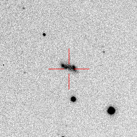
The first gain provided by the new imagery is a better estimate of the nebular sizes. Indeed, a significant increase ( $\geq$ 10″) in the previously stated dimensions (Paper I) is found for 13 objects when measuring their angular extent in the new H $\alpha$ and/or [N ii] images as listed in Table 3. In most cases, the increase in the measured size arises from the detection of faint bipolar outflows, outer structures or ansae previously missed in the IPHAS images. In the former case, the nebular emission formally considered as the whole PN is revealed to correspond to the brightest equatorial regions as illustrated in Figure 1 for Sab 2.

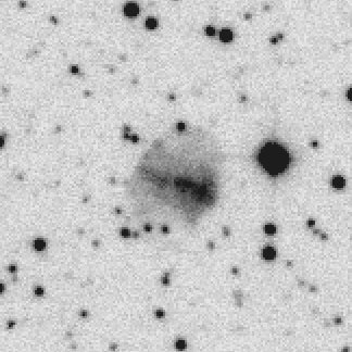
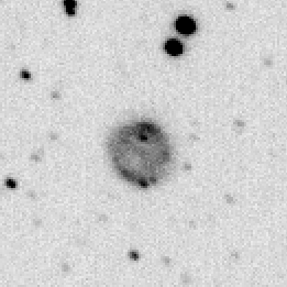
Then the combination of depth and improved spatial resolution reached by the new images allows the identification of small-scale features previously undetected or not obvious such as knots and filaments. Relatively compact knots are revealed in 11 objects, namely Sab 2 (Fig. 1), Sab 7, Sab 54, Sab 61, Sab 63, Sab 79, Sab 86, Sab 99, Sab 106, Sab 144, and J191104.8). Knots are mostly prominent in [N ii], except for highly ionized PNe where the knots emit mostly in [O iii] as is the case of Sab 63 (Fig. 2). Filaments are also detected in a number of sources, namely Sab 11, Sab 15, Sab 19, Sab 50, Sab 65 (Fig. 3), Sab 140, Sab 150, and Sab 157.

Actually, we have discarded Sab 15 (Fig. 5, 2^nd row) and Sab 50 (Fig. 7, 3^rd row) as genuine PNe based on their morphology. These are unlikely PNe, as their extended, irregular and highly filamentary nature reveal a morphology which mirrors more closely that of the shell of supernova remnants (SNRs) than PNe. They were first classified as possible PNe (the lowest grade of our classification scheme) based on the difficulty to have a clear detection from the spectroscopy. These two sources will not be discussed further.

More generally, the shallow IPHAS images provided limited information on the morphology of those PNe within the primary ERBIAS (Elliptical, Round, Bipolar, Irregular, Asymmetric and quasi-Stellar) and secondary amspr (a:one sided enhancement/asymmetries, m: multiple shells or external structure, p: point symmetry, r: well defined ring structure or annulus and s: resolved, internal structure) classification schemes (see Parker, et al. 2006). We have revised this morphology in the last column of Table 3, with most sources showing changes in their secondary amspr morphology and some of them even in their primary ERBIAS morphology. Here we note the introduction of the secondary classification key “w” to denote sources with a pinched, unresolved waist.

4.2 Ionization state of the PNe

The relative intensity of the H $\alpha$ , [O iii], and [N ii] emission lines can be used to assess the excitation degree of a PN. The images presented in Figures 4–15 are not flux-calibrated, however, and therefore they cannot be used to obtain a quantitative estimate of the nebular excitation. A qualitative assessment of nebular excitation can still be inferred from the comparison between the images in different emission lines in these figures as all images were obtained under photometric conditions through narrow-band filter sets with similar transmissions and using CCDs with similar responses. The relative contribution of these emission lines is immediately revealed in the colour-composite pictures obtained using similar intensity levels and contrast for the different emission lines: $R$ = [N ii], $G$ = H $\alpha$ , and $B$ = [O iii]. We shall define “red”, “green”, and “blue” PNe according to the prevalent colour in their colour-composite pictures.

The blue PNe are those completely dominated by [O iii] emission. The most obvious case is maybe Sab 7 (Fig. 4), but also Sab 118. We can add here PNe with a turquoise (blue+green) colour where H $\alpha$ has a non negligible contribution (e.g., Sab 44, Fig. 7). These blue and turquoise PNe are highly ionized sources that are expected to harbour the hottest PNe central stars (CSPNe) in this sample of sources. In a few cases, the blue and turquoise colours are dominant in the innermost regions, but green and mostly red (or their combination orange) prevail in the outer regions, thus revealing a notable ionization stratification. The most obvious case is possibly Sab 88 (Fig. 9), but also Sab 6, Sab 99 (Sabin et al. 2021), Sab 106, Sab 135, Sab 141, Sab 150, and Sab 151. This ionization stratification is suggestive of a hot CSPN with a limited ionizing flux, most likely an evolved CSPN already in the cooling track of white dwarfs.

On the opposite corner there is a number of red PNe, i.e., sources that are dominated by [N ii] emission. Among them, we can list Sab 11, Sab 23, Sab 36, Sab 39, Sab 81, Sab 109, Sab 130, Sab 139, and J191104.8 (Rodríguez-González et al. 2021). These objects can be associated with low excitation nebulae. An enhanced nitrogen content can be suggested, linking them to evolved Type I PNe, which is further supported by their bipolar or ring-like morphology.

We can add here also sources with an orange colour resulting from the combination of H $\alpha$ and [N ii] emissions, e.g., Sab 22, Sab 53, Sab 111, Sab 113, Sab 119, Sab 125, and Sab 138. Alternatively, orange sources may be heavily extinguished, thus reducing significantly the observed flux of the [O iii] emission line. Indeed, the much smaller number of field stars in the [O iii] images of some of them (e.g., Sab 53 and Sab 111) with respect to that in the H $\alpha$ and [N ii] images may be indicative of high extinction along the line of sight. The same can apply to some red sources (e.g., Sab 11), although in those cases it is not straightforward to disentangle the effects of low excitation and extinction, as both tend to diminish the relative intensity of the emission in the [O iii] line.

There is also a small group of green PNe (not to be confused in our scheme with those harboring the [O iii] ”green” line) whose emission is dominated by H $\alpha$ with nearly no [N ii] and little [O iii] emission, such as Sab 13 and Sab 44 and to some extent Sab 65. The significant shortfall of emission in the forbidden emission lines while H $\alpha$ is bright may be indicative of a recombining nebula.

Finally, we identify a white PN, namely Sab 148 (Fig. 14), whose colour-picture implies similar contributions of the three emission lines. Interestingly, this double shell PN shows low-ionization knots protruding along the major axis of the inner shell.

4.3 Classification and Deep Learning

Although the objects in this survey were selected as PNe, some may not be. Indeed, in Paper I some objects are classified as Likely or Possible. The HASH catalogue (Parker, Bojičić, & Frew 2016) classifies 51 of our targets as ’True PN’, four as ’Likely PN’, one as ’Possible PN’, and the two remaining objects are not classified as PN. The classification is based mainly on available survey images, aided by spectra.

Awang Iskandar et al. (2020) applied Deep Transfer Learning (DTL) to assign confidence levels to the HASH classifications. The network was trained on three sets of images available in HASH: optical H $\alpha$ images, quotient images (H $\alpha$ divided by the continuum image) and WISE images combining bands 2, 3, and 4 at 4.6 $\mu$ m, 12 $\mu$ m and 22 $\mu$ m, respectively. Each object was classified using each of the three resources. An object was classified as a true PN if at least two resources classified it accordingly. The DTL classified the majority of Likely PNe as PN (64%), but a smaller fraction of the Possible PNe (41%). This agreed with the expected higher level of confidence for the Likely PNe. In comparison, the model classified 94% of the True PN as PN.

We can now test how well the DTL output agrees with the deeper images presented here. The trained network of Awang Iskandar et al. (2020) with the Densenet201 algorithm was used. Densenet201 uses 201 layers, and differs from other tested implementations by making the input feature map reusable and accessible to later layers (Huang et al. 2017). In the tests of Awang Iskandar et al. (2020) it was found to be among the most effective algorithms for the current purpose. We applied this to the HASH images of the 58 objects in this catalogue. An object was classified as a PN if at least two image types returned this classification. The three methods agree on a PN classification for 40 out of the 58 objects in this sample and it was questioned only by one criterion for seven objects, thus leading to a PN classification for 47 sources. Eleven sources were thus rejected as PN, in 3 cases by all three criteria.

Table 4: Objects for which the classification as PN is not certain

Sab #	HASH	DTL	deep image	comment
2	true	not	true
13	true	not	true
15	possible	not	not	supernova remnant
19	true	true	possible	unusual structure; very low luminosity for PN star
22	likely	true	true
31	true	not	true	very faint
36	likely	true	possible	too faint to classify
42	true	not	possible	no morphological information
50	not	not	not	supernova remnant
53	not	not	possible	Star too red to be a PN central star
61	true	not	possible	very elongated. Jet, PN or YSO?
81	true	not	true
99	true	true	possible	asymmetric
108	likely	true	possible	lack of symmetry suggestive of ISM
119	likely	true	true
125	true	not	possible	not fully symmetric
138	true	not	true
140	true	true	possible	Irregular halo

The 18 objects for which either the HASH database, the DTL or the current images leaves some doubt about the identification as PN are listed in Table 4.
Most of them are likely to be PNe, but we cannot be fully confident about it. A few nebulae are too faint to confidently classify them. Here deeper images would certainly help. The HASH and deep image classification agree for five objects, but the DTL does not. In most of those cases the deep images reveal structure which make a PN classification very likely. Irregular structures are likely to lead to a DTL classification as non-PN, although PNe can become irregular during late stages of their evolution due to ISM interactions. Anyhow it casts lower confidence in the classification as other ISM structures also often are irregular.

Two objects are confirmed as non-PN (15, 50), both very likely supernova remnants. Sab 53 is unlikely to be a PN and may be related to symbiotic stars. This might also be the case of Sab 61, which has a very unusual structure for a PN and needs further study. Finally, Sab 19 is classified as a true PN in the detailed study of Guerrero et al. (2021).

5 Conclusion

This paper presents a new set of deep images for 58 True, Likely and Possible extended PNe detected with IPHAS. These new images have been obtained using H $\alpha$ , [N ii] $\lambda$ 6584 Å, and [O iii] $\lambda$ 5007 Å narrow-band filters.

The depth of these images in different emission lines has allowed us to detect macro- and micro-structures in these PNe such as outflows, filaments as well as knots and ansae. These new features has led us to the morphological reclassification of some sources. Two sources originally catalogued as Probable PNe have even been discarded as PNe based on their filamentary nature most likely implying a SNR nature. In some cases we were able to uncover the full extent of the optical nebulae with an update on the total size.

The images presented here also indicate that these PNe span over a large excitation or ionization range from the Type-I like PNe (N-enhanced) to the highly ionized PNe, highlighting the wide and rich range of IPHAS objects. Indeed, our blue ([O iii] dominated), red ([N ii] dominated), green (H $\alpha$ dominated) and white (similar contribution in all filters) qualitative classification of PNe is indicative of the different characteristics of the ionizing central stars as well as their evolutionary status. We note, however, that images acquired through the [O iii] filter are more prone to extinction effects, which may affect the above classification.

We also used Deep Transfer Learning for the automated classification of the objects owing that our sample includes True, Likely and Possible PNe. These results were compared to the classification performed using the HASH catalogue as well as our deep images. Most of the objects are thus classified as PNe by all three methods and amongst the 18 doubtful cases it appears that our deep images are very useful, if not critical, mostly in the case of the faintest and more irregular PNe.

This first imaging catalogue is therefore a valuable tool to support further more exhaustive studies of these PNe (hence the analysis of a group of such PNe has already been carried on by Corradi et al. 2011; Miszalski, Boffin, & Corradi 2013; Guerrero et al. 2021; Rodríguez-González et al. 2021; Sabin et al. 2021) and we expect to proceed to the deep imaging of the full catalogue presented in our Paper I.

Acknowledgements

We thank the referee for the his/her comments which help improving the paper. LS acknowledges support from PAPIIT grant IN-101819 (Mexico). MAG acknowledges support from grant AYA PGC2018-102184-B-I00 co-funded with FEDER funds. GR-L acknowledges support from CONACyT (grant 263373) and PRODEP (Mexico). JAT acknowledges funding by Dirección General de Asuntos del Personal Academico of the Universidad Nacional Autónoma de México (DGAPA, UNAM) project IA100720 and the Marcos Moshinsky Fundation (Mexico). AAZ acknowledges funding from STFC under grant number ST/T000414/1 and Newton grant ST/R006768/1, and from a Hung Hing Ying visiting professorship at the University of Hong Kong. DNFAI acknowledges funding under ‘Deep Learning for Classification of Astronomical Archives’ from the Newton-Ungku Omar Fund: F08/STFC/1792/2018.

This work is partially based on observations made with the Nordic Optical Telescope, operated by the Nordic Optical Telescope Scientific Association installed in the Spanish Observatorio de El Roque de los Muchachos of the Instituto de Astrofísica de Canarias in La Palma, Spain, and the Aristarchos telescope, which is operated at the Helmos Observatory by the IAASARS of the National Observatory of Athens. This paper makes use of data obtained as part of the INT Photometric H $\alpha$ Survey of the Northern Galactic Plane (IPHAS, www.iphas.org) carried out at the Isaac Newton Telescope (INT). The INT is operated on the island of La Palma by the Isaac Newton Group in the Spanish Observatorio del Roque de los Muchachos of the Instituto de Astrofísica de Canarias. All IPHAS data are processed by the Cambridge Astronomical Survey Unit, at the Institute of Astronomy in Cambridge. The bandmerged DR2 catalogue was assembled at the Centre for Astrophysics Research, University of Hertfordshire, supported by STFC grant ST/J001333/1. This work has made extensive use of NASA’s Astrophysics Data System.

Data availability

The images here presented will be included in due time in the HASH database (http://202.189.117.101:8999/gpne/index.php), once an option currently under development to download the best available optical images of PNe will become available. In the meantime the data presented in this work are available on request to the first author.

References

Awang Iskandar et al. (2020) Awang Iskandar D. N. F., Zijlstra A. A., McDonald I., Abdullah R., Fuller G. A., Fauzi A. H., Abdullah J., 2020, Galax, 8, 88. doi:10.3390/galaxies8040088
Corradi et al. (2011) Corradi R. L. M., Sabin L., Miszalski B., Rodríguez-Gil P., Santander-García M., Jones D., Drew J. E., et al., 2011, MNRAS, 410, 1349.
Drew, et al. (2005) Drew J. E., et al., 2005, MNRAS, 362, 753
Guerrero et al. (2021) Guerrero M. A., Ortiz R., Sabin L., Ramos-Larios G., Alfaro E. J., 2021, MNRAS, 501, 3594.
Huang et al. (2017) Huang G., Liu S., van der Maaten L., Weinberger K. Q., 2017, Proc. IEEE Conf. on Computer Vision and pattern Recognition, pp. 2261-2269. arXiv:1711.09224
Manchado et al. (1996) Manchado A., Guerrero M. A., Stanghellini L., Serra-Ricart M., 1996, iacm.book
Mampaso et al. (2006) Mampaso A., Corradi R. L. M., Viironen K., Leisy P., Greimel R., Drew J. E., Barlow M. J., et al., 2006, A&A, 458, 203.
Meaburn et al. (2003) Meaburn, J., López, J. A., Gutiérrez, L., et al. 2003, Rev. Mex. Astron. Astrofis., 39, 185
Miszalski, Boffin, & Corradi (2013) Miszalski B., Boffin H. M. J., Corradi R. L. M., 2013, MNRAS, 428, L39.
Monguió et al. (2020) Monguió M., Greimel R., Drew J. E., Barentsen G., Groot P. J., Irwin M. J., Casares J., et al., 2020, A&A, 638, A18.
Parker, et al. (2006) Parker Q. A., et al., 2006, MNRAS, 373, 79.
Parker, Bojičić, & Frew (2016) Parker Q. A., Bojičić I. S., Frew D. J., 2016, JPhCS, 728, 032008. doi:10.1088/1742-6596/728/3/032008
O’dell, et al. (2003) O’dell C. R., Balick B., Hajian A. R., Henney W. J., Burkert A., 2003, Rev. Mex. Astron. Astrofis., 15, 29.
Rodríguez-González et al. (2021) Rodríguez-González J. B., Sabin L., Toalá J. A., Zavala S., Ramos-Larios G., Guerrero M. A., Parker Q. A., et al., 2021, MNRAS, 501, 3605.
Sabin, et al. (2014) Sabin L., et al., 2014, MNRAS, 443, 3388
Sabin et al. (2021) Sabin L., Guerrero M. A., Zavala S., Toalá J. A., Ramos-Larios G., Gómez-Llanos V., 2021, MNRAS, 501, 3582.
Stanghellini, Shaw, & Villaver (2016) Stanghellini L., Shaw R. A., Villaver E., 2016, ApJ, 830, 33. doi:10.3847/0004-637X/830/1/33
Tody (1993) Tody, D. 1993, Astronomical Data Analysis Software and Systems II, 52, 173

Appendix A Images

In this appendix we present all the H $\alpha$ , [N ii], [O iii] narrow-band images of all objects studied in this paper. In addition a colour-composite image combining these three filters is also presented for each object. The images are presented in Figures 4–15. We note that the images of J191104.8 (Fig. 15), Sab 19 (Fig. 5) and Sab 99 (Fig. 9) were presented in Rodríguez-González et al. (2021), Guerrero et al. (2021) and Sabin et al. (2021), respectively.