Benchmarking variational quantum eigensolvers for the square-octagon-lattice Kitaev model
Abstract
Quantum spin systems may offer the first opportunities for beyond-classical quantum computations of scientific interest. While general quantum simulation algorithms likely require error-corrected qubits, there may be applications of scientific interest prior to the practical implementation of quantum error correction. The variational quantum eigensolver (VQE) is a promising approach to finding energy eigenvalues on noisy quantum computers. Lattice models are of broad interest for use on near-term quantum hardware due to the sparsity of the number of Hamiltonian terms and the possibility of matching the lattice geometry to the hardware geometry. Here, we consider the Kitaev spin model on a hardware-native square-octagon qubit connectivity map, and examine the possibility of efficiently probing its rich phase diagram with VQE approaches. By benchmarking different choices of variational ansatz states and classical optimizers, we illustrate the advantage of a mixed optimization approach using the Hamiltonian variational ansatz (HVA) and the potential of probing the system’s phase diagram using VQE. We further demonstrate the implementation of HVA circuits on Rigetti’s Aspen-9 chip with error mitigation.
I Introduction
In the context of quantum computation there is reason to believe the quantum simulation of spin systems may offer early results in the search for beyond classical computations of real scientific interest [1]. Although beyond-classical calculations that offer truly new insights into scientific problems will likely require quantum error correction (QEC) [2, 3], it may be possible to find approachable questions of scientific interest even before the advent of full QEC if we carefully pair the computing hardware and problem. Lattice models are a natural class of systems to consider in this regard, and they also tend to have sparse Hamiltonian representations that require fewer quantum resources than other Hamiltonian models [4]. In this paper, we consider a spin model [5, 6] that maps naturally onto the square-octagon qubit connectivity of a superconducting quantum processor and perform an open study of the most efficient ways of finding the ground state of this system using variational quantum algorithms based on parameterized quantum circuits.
The near-term, so-called “Noisy Intermediate Scale Quantum” (NISQ) [7, 8, 9] computing era is defined by the conditions imposed by noisy quantum hardware. Decoherence errors mandate the use of “shallow” quantum circuit programs, i.e., quantum circuits with a small number of consecutive operations on the qubit register array. Quantum noise also currently limits the effective “width” of a circuit, which is governed by the total number of qubits deployed. A wide circuit consists of more quantum gates than a narrow circuit, and thus the gate error rates effectively limit how wide a circuit could be before the result becomes no longer useful with the decreasing circuit fidelity.
The variational quantum eigensolver (VQE) [10, 11, 12, 13, 14, 15, 16, 17, 18] is an algorithm that seeks to implement low-depth variational ansatz circuits to find eigenstates of complex many-body Hamiltonians. Different approaches to VQE entail different choices of ansatz circuits, which take into account different figures of merit. These can include reducing the circuit depth, increasing the accuracy or wavefunction fidelity, or minimizing the number of variational parameters. To match these varied goals, there are many different approaches which include hardware efficient ansaetze (HEA) [13], adaptive ansaetze [14, 17, 16, 19, 20, 21, 22], and ansaetze inspired by classical simulations [13, 17, 23]. One particular ansatz of interest is the Hamiltonian variational ansatz (HVA) [24]. This ansatz draws from ideas expressed by the quantum approximate optimization algorithm and adiabatic quantum computation [25, 26]. Recent work [27] suggests the HVA may be less prone to problems with “barren plateaus” [28] and therefore easier to optimize than the HEA (see, however, Ref. [29]).
Kitaev spin models [5, 30, 31], which are a family of frustrated quantum spin models with bond-dependent interactions, provide an intriguing testbed for NISQ quantum simulation. Kitaev models can be defined on arbitrary trivalent graphs and are appealing due to their exact solvability via a mapping to free Majorana fermions [5]. Despite their simplicity, they yield a rich variety of phases, including gapped and gapless U(1) spin liquids [32]. In a magnetic field, Kitaev models support non-Abelian Ising anyons [5], which (in addition to the aforementioned spin-liquid phase) makes them a promising platform for topological quantum computation [33, 34, 35]. Kitaev-like models are predicted to arise in spin-orbit-coupled Mott insulators [36], and a plethora of materials candidates exist [31]. Putative signatures of spin-liquid physics have been observed in neutron scattering [37, 38] and thermal transport measurements [39, 40].
In realistic systems, the desired “Kitaev interactions” compete with more mundane (e.g. Heisenberg) interactions and external magnetic fields, all of which spoil the Kitaev model’s exact solvability and often favor magnetically ordered ground states. One therefore must resort to numerical methods [41, 42, 43, 44, 45, 46, 47, 48, 49, 50, 51, 52, 53, 54, 55], such as exact diagonalization (ED), tensor-network techniques like the density-matrix renormalization group [56, 57, 58], and Monte Carlo [59, 60], to study the ground-state phase diagram. Thus, Kitaev models provide a useful benchmark for near-term quantum algorithms for the study of interacting quantum systems.
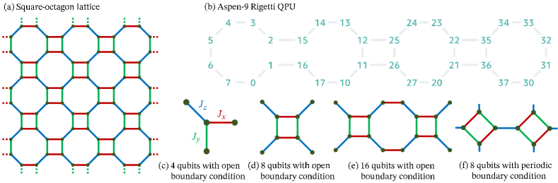
In this paper, we focus on the Kitaev model on the square-octagon lattice [6, 61], which maps natively with minimal compilation overhead onto Rigetti’s Aspen architecture featuring 32 transmons with a square-octagon topology on the Aspen-9 chip used in this paper [62, 63, 64]. This native mapping makes the quantum simulation of the square-octagon Kitaev model a potential NISQ application of the Aspen-9 quantum processing unit (QPU) to carry out quantum computing calculations without full QEC. We will benchmark the variational ansaetze and optimization algorithms to determine the ground state of the Kitaev model with and without a magnetic field. Supported by the results of classical simulations, we will illustrate a mixed optimization approach using both a local optimizer and a non-local optimizer started with multiple initial values. This opens up the possibility of using VQE calculations to probe the phase diagram of the Kitaev model in the presence of a magnetic field or other perturbations away from the solvable limit. Together with an experimental test run of classically optimized VQE circuits on the QPU, this paper provides insights into the appropriate VQE approach for further VQE experiments with a system size beyond the capability of classical computation.
This paper is organized as follows. In section II.1, we review the Kitaev model on the square-octagon lattice and its phase diagram in the presence of a magnetic field. This is followed by a review of VQE approaches in section II.2. We discuss our methodology for investigating the circuit ansaetze (section III.2) and optimizers (section III.3), and for implementing the classically optimized circuits on Aspen-9 with noise mitigation (section III.5). The results of the paper are then discussed in section IV.
II Background
II.1 Square–octagon-lattice Kitaev model
| Label | Model parameters | Ground-state energy | |||||||
|---|---|---|---|---|---|---|---|---|---|
| TCz | 0.1 | 0.1 | 1 | 0 | 0 | 0 | -1.0100 | -4.0100 | -8.0250 |
| TCz+ | 0.1 | 0.1 | 1 | -1.1723 | -4.2476 | -8.5002 | |||
| GL | 1 | 0 | 0 | 0 | -1.4142 | -4.4721 | -9.3002 | ||
| GL+ | 1 | -1.5831 | -4.7011 | -9.7008 | |||||
The ferromagnetic Kitaev model on the square-octagon lattice has the Hamiltonian,
| (1) |
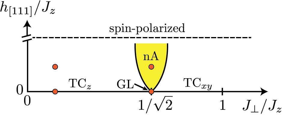
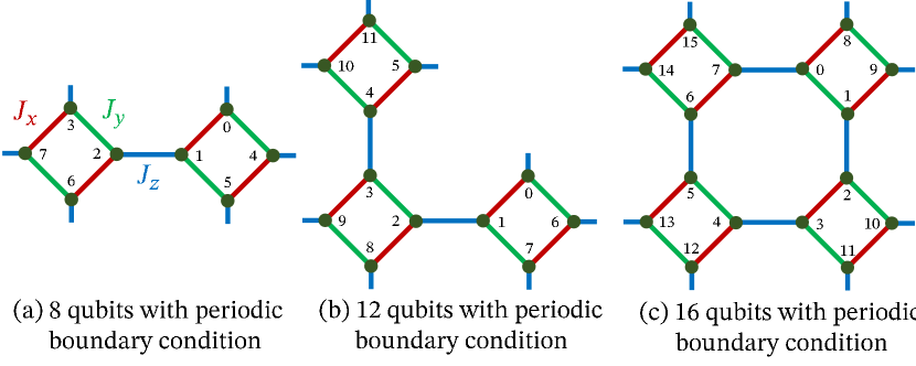
where and we partition the nearest-neighbor bonds of the lattice into and sets depending on their orientation (see Fig. 1(a)), and are the Pauli matrices for site . Like the original honeycomb-lattice version, the Kitaev model on the square-octagon lattice is exactly solvable by mapping to free fermions [6]. To move beyond the exactly solvable limit and explore the rich phase diagram emerging in finite magnetic field (see Fig. 2), we consider the model
| (2) |
where is the magnetic field. This Hamiltonian and variants thereof have been studied in Refs. [6, 61, 65, 66, 67, 68, 69] using a variety of methods, and the general features of its phase diagram are well understood.
At zero field, the model features two gapped spin-liquid phases, which we dub and . The phase can be understood perturbatively in the limit , where an effective Hamiltonian equivalent to the well-known toric code [70] emerges [6, 61]. The phase can be understood in the opposite limit , where perturbation theory yields [61] a Hamiltonian equivalent to the so-called Wen-plaquette model [71], which is in turn equivalent to the toric code [72, 73]. In both phases, the model has topological order and supports Abelian anyonic excitations with nontrivial mutual statistics; nevertheless, the phases are distinct [61, 67]. A critical line separating these two gapped phases appears at .
At small but finite field, the phases persist [66], as is expected due to the gapped nature of these phases. Provided that none of , the gapless line at gives way to a gapped phase with non-Abelian Majorana excitations [6]. At large field, the system enters a trivial spin-polarized paramagnetic phase. The phase diagram of the square-octagon Kitaev model in a field has been studied in Refs. [6, 65, 66], but a detailed understanding of the location of all transitions is lacking. A schematic of the phase diagram for in a -oriented field is shown in Fig. 2.
In the following, we focus on a number of representative points in the phase diagram, which are highlighted in Fig. 2 and defined in Table 1. The table also includes the exact ground-state energies for these parameters that are obtained using ED, which we will use to benchmark our VQE results. We consider lattices with open boundary conditions shown in Fig. 1(b,c,d) for the benchmarks.
II.2 VQE
VQE algorithms prepare the eigenstates of the system Hamiltonian by optimizing the cost function associated with a trial state , which is prepared by a parametrized circuit ansatz such that , where is a chosen reference state [11, 13]. To prepare the ground state, the VQE algorithm minimizes, using a classical optimizer, the energy of the trial state, i.e.,
| (3) |
The cost function is measured on the QPU, and the result is fed into the classical optimizer, making the VQE a hybrid quantum-classical approach. Several different approaches are possible for calculating excited states [10, 12, 74, 16]. One approach is to minimize a modified cost function including the overlaps with the lower-energy eigenstates determined in the previous iterations [75, 76].
Similar to other variational algorithms, the output of VQE only approximates the eigenstates of , and the quality of the solution depends on the choice of ansatz. The true ground state cannot be expressed by the trial state if an inappropriate ansatz is chosen, resulting in an approximated energy much higher than the true ground-state energy. The success of VQE algorithms hence strongly depends on the circuit ansatz. Optimizing a generic HEA is a challenging task for several reasons, including barren plateaus [28] and sensitivity to the optimizer meta-parameters [77]. The challenge of optimization grows even bigger with the rapidly increasing number of variational parameters with the system size. The HVA, built using rotations generated by Hamiltonian terms, has been suggested to be a more efficient option than HEA in certain cases [27], as has been observed in several numerical simulations [78, 79, 77]. Later in this paper, we will compare the effectiveness of these two ansaetze in preparing the ground state of the square-octagon Kitaev model with 8 and 16 qubits.
The choice of classical optimization algorithm plays an important role in VQE implementations as well. Picking an inappropriate optimizer results in a slow convergence rate (and thus a longer QPU runtime), if it ever converges to a sufficiently good minimum at all [80, 81, 82, 77]. We will also benchmark the efficiency of a few optimizers using the Kitaev model to provide some insights into the VQE optimization strategy.
III Methodology
III.1 Overview of approach
In the following sections we review our theoretical and experimental approaches to studying VQE simulations of the Kitaev model. Our paper first aims, via classical simulations, to understand the modeling requirements for obtaining different phases of the Kitaev model with various ansaetze and optimizers, and then tests these approaches on present-day quantum hardware. In this paper, we classically simulate the quantum programs using PyQuil [83], Cirq [84] and Qiskit [85], and we execute classically optimized quantum circuits on Rigetti’s Aspen-9 QPU.
III.2 VQE Ansatz
The QPUs are initialized in a chosen reference state with all physical qubits being at zero in the computational basis. The ansatz trial state is prepared by two classes (HVA and HEA) of parametrized circuit ansatzes to be discussed in this section.
We construct the HVA using the Kitaev couplings , and in Eq. (1), and the magnetic fields , and in the Eq. (2). The HVA represented by the unitary matrix has layers such that
| (4) |
Each layer consists of the exponentiation of the Kitaev couplings and the magnetic fields multiplied by the parameters such that
| (5) |
The two-qubit gate count of each HVA layer scales linearly with the number of qubits. (For an infinite square-octagon lattice, .) The Aspen-9 connectivity shown in Fig. 1(b) is natively the square-octagon lattice. One HVA layer can then be executed with CPHASE gates supported natively by Aspen-9 [64]. If we execute the circuit on a QPU with a different two-dimensional connectivity, an overhead of SWAP gates will be required for implementing the HVA. Although this overhead does not change the overall gate complexity of the HVA implementation, it can still be quite demanding for NISQ devices. Using the Aspen-9 QPU with the native connectivity thus provides a significant advantage in the near term.
There are six parameters for each HVA layer, independent of the system size . This makes the optimization of the HVA straightforward to analyze with increasing system size. We can make a rough estimate of how many times the cost function has to be evaluated based on the results on smaller lattices with a similar number of layers. Nonetheless, if the ground state of a larger system exhibits longer-range entanglement, more layers will typically be needed to achieve the same degree of accuracy as in a smaller system. Hence, the required number of layers and the total number of parameters depend on the system size, and usually can only be determined by testing. This makes the prediction nontrivial especially when we consider small lattices in Fig. 1 with noticeable finite-size effects.
Other than HVA, we consider the HEA which is widely used in NISQ applications [13, 86, 87]. The general principle of the HEA is to construct circuit ansaetze using the native gates supported by the QPU, and hence different specific forms of the HEA are constructed targeting different QPUs. For Aspen-9, the native gate set consists of the XY gate [63], the CPHASE and CZ gates [64] as well as the single-qubit gates and with . Moreover, the Quil programming language [83] and its accompanying optimizing compiler Quil-C [88] on the Rigetti stack [89] admit parametric compilation, which allows for the ansatz to be compiled only once, so that the numerical values of the ansatz parameters are only updated at runtime, without the need of incurring the compilation overhead at every step of the optimization process. This allows for faster execution times and feedback loops between the quantum and classical processors in the hybrid computation.
Roughly speaking, a HEA usually consists of layers of parameterized single-qubit rotations and two-qubit gates to create entanglement between qubits. Adopting this idea with respect to the Aspen-9 native gate set and its connectivity, we consider two ansaetze, namely the HEA-CZ using CZ gates and single-qubit rotation gates, and the HEA-XY using XY gates and single-qubit rotation gates. Here, we focus on the native two-qubit gates (CZ and XY) and slightly relax the native restriction on the single-qubit gates since the single-qubit gates have a much lower error rate than the two-qubit gates. The unitary representation of an -layer HEA is given by
| (6) |
Here, the layer preparing each qubit in an arbitrary unentangled state is given by
| (7) |
Note that an arbitrary single-qubit rotation is represented by the gate sequence . The rightmost can be omitted here since the qubits are initialized in the zero-state and just gives an irrelevant global phase. The other layers then entangle the qubits using the two-qubit gates. For HEA-CZ, we have
where represents the hardware-native connectivity. Similarly, for HEA-XY, we have
Once again, the sequence represents an arbitrary single-qubit rotation. For HEA-CZ, since commutes with , the first can be combined with the last in the previous layer. thus requires two fewer single-qubit gates for HEA-CZ than for HEA-XY.
In the present case, with the native connectivity being the same as the lattice geometry, the number of two-qubit gates of the HEA scales as , which is the same as for the HVA, as expected. On the other hand, the number of parameters per layer also scales linearly with , in contrast to the constant scaling of the HVA. The much larger number of parameters makes the HEA more expressive especially when a small number of layers is used. However, this also makes the HEA hard to scale up since optimizing a large number of parameters is challenging for non-convex cost functions.
III.3 Optimizers
| Optimizer | Gradient-free | Genetic | Local |
| BFGS | ✓ | ||
| BOBYQA [91] | ✓ | ✓ | |
| CMA-ES [95] | ✓ | ✓ | |
| Dual Annealing [96] | ✓ | ||
| SPSA [97] | ✓ |
The cost function associated with VQE algorithms is in general non-convex with many local extrema. Similar to optimizing other classical non-convex cost functions, it is typically hard to decide on an efficient optimizer a priori [98]. To make our benchmark less dependent on a specific choice of the optimizer, we will test the list of optimizers shown in Table 2. This list consists of a few well-known gradient-free algorithms (BOBYQA, CMA-ES, dual annealing), gradient-based optimizers (SPSA, BFGS), non-local optimizers (CMA-ES, dual annealing), and a genetic algorithm (CMA-ES). Even though this is far from a comprehensive list, we can gain insight into how different types of optimizers work for our specific VQE cost function.
We compute the gradients needed for the gradient-based optimizers by finite-difference methods, which require an additional measurement of the cost function using the QPU for each gradient . This makes the cost of running these gradient-based optimizers larger than for the gradient-free algorithms, making them suboptimal given the limited clock rate of present-day QPUs. More efficient quantum algorithms to evaluate gradients have attracted great interest recently [99, 100, 101, 102]. For instance, the parameter-shift rule allows the gradients to be evaluated with an analytic expression without introducing overhead in circuit depth or circuit width [101]. The analytical evaluation will improve the performance of the optimization with noise. However, using the parameter-shift rule for the HVA ansatz requires a generator decomposition [103], which makes the number of required expectation-value measurements scale with the system size (compared to constant scaling for finite-difference methods). Other algorithms usually require ancilla qubits and/or extra gate operations, and thus are challenging to implement on NISQ devices. Nonetheless, once QPUs with better gate fidelities and coherence properties are available, further studies will be required to revisit these results and strike a balance between quantum resource requirements and optimization efficiency.
III.4 Determining energy gap by VQE
The energy gap between the ground state and the first excited state is a useful quantity in probing the system’s phase diagram. VQE algorithms can obtain excited states by modifying the cost function with an additional term penalizing the overlap between the trial state and the lower-energy state obtained previously [76]. In particular, to determine the energy gap, we use the following cost function to determine the next excited state beyond the ground state,
| (8) |
where is the penalty weight and are the optimal parameters corresponding to the ground state previously determined by VQE. The overlap can be experimentally determined on QPUs by executing the circuit corresponding to and then measuring the population of the zero state . The penalty weight is chosen to be larger than any relevant energy gaps, and we choose it to be 0.3 in our numerical experiment.
III.5 Experiment and noise mitigation
We run pre-optimized HVA circuits with one layer (HVA-1) on four- and eight-qubit sub-lattices of Rigetti’s Aspen-9 QPU. The variational optimization of the HVA is first performed on a classical simulator, and the circuits are then run on the QPU for the optimal choice of parameters. While this approach circumvents the hybrid quantum/classical computation, it nevertheless serves as a benchmark for how well the quantum processor performs in proof-of-concept experiments. For comparison, recent state of the art results for many body Hamiltonian simulations have opted for either purely classical optimization instead of a VQE step [104] or running their algorithms on smaller numbers of qubits [23, 105].
| Qubits | Optimizer | Error in energy | Cost function evaluations |
|---|---|---|---|
| 8 | BFGS, 501 initial values | 0.00094 | mean: 5352, max: 10865 |
| 16 | BFGS, 501 initial values | 0.02672 | mean: 5569, max: 10186 |
| 8 | BOBYQA, 501 initial values | 0.00045 | mean: 1099, max: 1920 |
| 16 | BOBYQA, 501 initial values | 0.01744 | mean: 1255, max: 3049 |
| 8 | CMA-ES | 0.00015 | 43290 |
| 16 | CMA-ES | 0.04036 | 49335 |
| 8 | CMA-ES, 80 initial values | 0.00005 | mean: 20528, max: 83590 |
| 16 | CMA-ES, 80 initial values | 0.01327 | mean: 27504, max: 73138 |
| 8 | Dual annealing | 0.00252 | 100000 (cutoff) |
| 16 | Dual annealing | 0.04634 | 100106 (cutoff) |
| 8 | SPSA | 0.04500 | 100000 (cutoff) |
| 16 | SPSA | 0.08145 | 100000 (cutoff) |
We perform digital zero-noise extrapolation (ZNE) [106, 107, 108] by first exaggerating the errors in the circuit by replacing a subset of CZs by an odd multiple of them. We choose such subsets to increase the total CZ count in the circuit by a factor of . For each scale factor , we run 25-100 (four qubits) and 100 (eight qubits) different circuit implementations for 1000 shots each. For the four-qubit case, we pick The bare HVA-1 circuit, with six CZs, corresponds to . To obtain , we note that the exponentials of each of the two-local terms (, and ) are compiled to two CZs, along with a few one-qubit gates. For , we replace the first of the two CZs compiling the exponential of the term with three CZs, then again for the and terms, then take the average of all three types of circuits to get an estimated expectation value of the cost Hamiltonian. For , we replace both the CZs with three CZs each, once for each of the three two-local terms. For , we replace both CZs in the term, and the first of the two CZs in the term with three CZs each for one experiment, and for another we replace both CZs in the term and the second of the two CZs in the term with three CZs each. Finally, for , we perform three experiments, in which we replace the CZs in the and , and , or and exponentials with three CZs each.
For the eight-qubit case, we choose . For , we have a total of 16 CZs, two for each of the edges. For , we run 25 different circuits for each of the scenarios where we replace (a) every CZ in the -links with three CZs, (b) every CZ in the -links with three CZs, (c) every CZ in two of the four -links with three CZs, and (d) every CZ in the remaining two of the four -links with three CZs. For , we run 50 different circuits for each of the scenarios where we replace (i) every CZ in the - and -links with three CZs, and (ii) every CZ in the -links with three CZs. For (), we simply take 100 different circuits where we replace every CZ in the circuit with three (five) CZs.
For each of the circuit implementations in each scale factor family, we estimate the cost function (3) by measuring the expectation values of all Pauli strings given in eq. 2. Each of these expectation values associated with qubits is determined experimentally by applying suitable single-qubit gates to transform any Pauli or Pauli to Pauli followed by a projective measurement over the computational basis. The measured probability distributions are subjected to readout errors which can be mitigated as follows. The readout errors can be modeled by classical Markovian process [109] described by the equation
| (9) |
Here, is the confusion matrix that relates the probability distribution of the prepared state without readout error and the probability distribution experimentally measured with readout error. Each element of can be interpreted as the conditional probability of measuring the bitstring given that the bitstring is prepared. In our experiment, is estimated by preparing a bitstring, then computing the fraction of each of bitstrings from 10,000 shots to estimate the conditional probabilities, then repeating this procedure for all bitstrings. By inverting , we obtain a readout error mitigated estimate of the probability of outcomes of all bitstrings using
| (10) |
In turn, these lead to readout-error-mitigated estimates of the cost function (3) in each of the 100 circuits for any given family associated with a scale factor. We then average these expectation values over all 100 circuits to produce a single value representing the family of circuits associated with a given scale factor. These representative values are then plotted against the scale factors, and a polynomial fit is found to extrapolate to the (zero noise) limit to obtain an estimate of the cost function mitigated for both gate and readout errors.
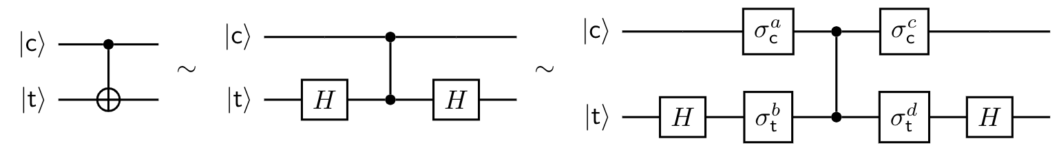
For the eight-qubit case, we also perform randomized compilation [110] to twirl the physical error channels into stochastic errors to improve the result. In the HVA, the exponential of every two-body term can be compiled using two native CZs. Before each CZ gate, we apply random Pauli operators , where and the subscripts and denote the control and target qubits, respectively. After applying the CZ unitary 111Note that the same unitary can also be written , so that the CZ gate remains invariant if we swap the labels and . Therefore, it doesn’t matter how we assign the labels control/target to the two qubits participating in this interaction., we apply Pauli operators such that . Following Ref. [106], this is given by
| (11) | ||||
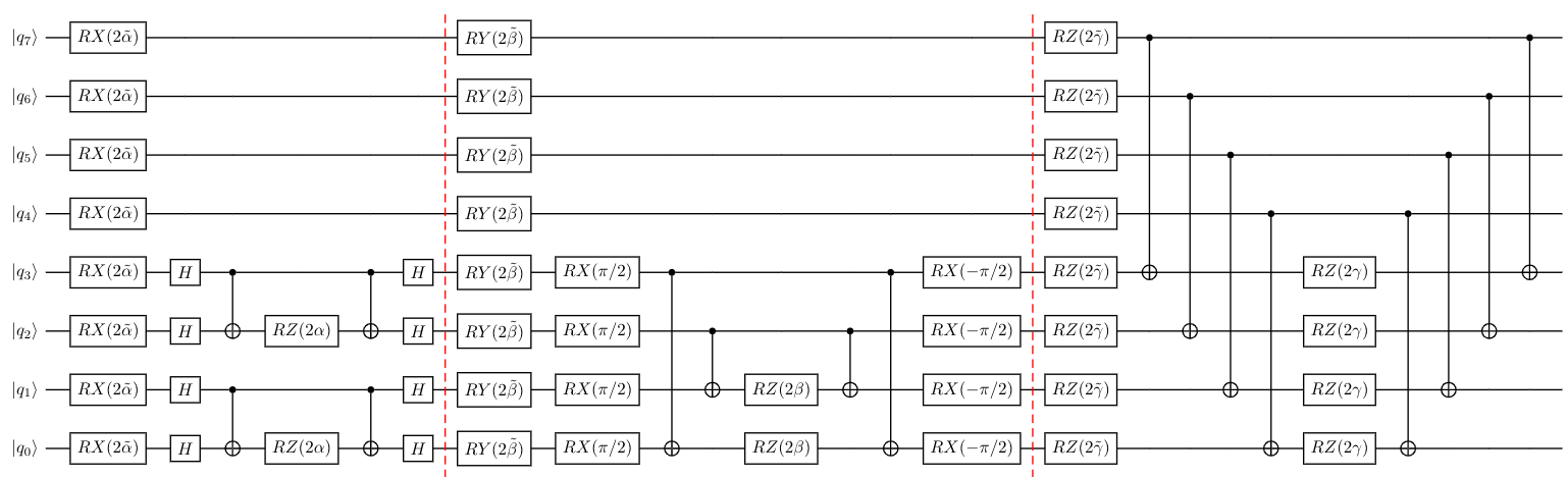
This noise tailoring makes the errors more well behaved and better suited for error mitigation techniques such as ZNE [106, 112, 113, 114]. A schematic circuit for the HVA with one layer on an eight-qubit sub-lattice is shown in Fig. 3. The twirling operation is depicted in Fig. 4.
For twirled experiments we take point-estimates of the expectation values for many circuit implementations for each scale factor and feed them into a Bayesian linear regression model implemented in Turing.jl [115] with Gaussian priors for slope and intercept and a truncated-at-zero Gaussian prior for the variance, and we run Markov Chain Monte Carlo (MCMC) until well converged. Hyperparameters of the priors were all set to mean zero and standard deviation 1000 (i.e. no prior information or preference over the reasonable range of the parameters), but these hyperparameters had negligible impact on the posterior distribution so long as they were not set to effectively exclude the region of the observed data. MCMC was run with a No U-Turn Sampler [116] for iterations, we exclude the first 3000 to exclude any warmup period, and for all runs we had an effective remaining sample size . For untwirled experiments, we follow the same basic procedure but incorporate shot noise for each circuit implementation by performing a Bayesian bootstrap [117] over the shot data to produce an estimate and uncertainty for the expectation value from each circuit implementation. We then feed those estimates and uncertainties into the Bayesian linear regression defined above.
IV Results
IV.1 Statevector simulations
We test the optimizers listed in Table 2 using the cost function (3) associated with the four-layer HVA for the eight-qubit and 16-qubit lattices shown in Fig. 1 and the parameter choice (GL + ) in Table 1. This cost function has 24 parameters to be optimized. The results using a statevector simulator are summarized in Table 3.
BFGS and BOBYQA are susceptible to local extrema and their performance highly depends on the initial choice of the parameters. We employ a multiple-initial-condition strategy and randomly pick 501 initial parameter values to start with. In general, the number of initial values required for a good result will increase with the number of parameters of the cost function. BOBYQA gives a smaller error in energy compared to BFGS in both eight-qubit and 16-qubit tests, and BOBYQA also converges much faster than BFGS, which requires the costly computation of gradients by finite-difference methods. The other local optimizer, SPSA, is less susceptible to local extrema due to its stochastic nature. However, its convergence is slow and will require many iterations in order to achieve good accuracy. Among the local optimizers, BOBYQA with multiple initial values gives the best performance in terms of both the accuracy of the result and the speed of convergence.
CMA-ES and dual annealing are non-local optimizers that are able to escape from local extrema. Table 3 shows that both optimizers converge toward a minimum with energy close to the exact value even starting from just one initial value. CMA-ES consistently converges faster among the two. Obtaining the best performance from CMA-ES requires fine tuning of the optimizer meta-parameters, which depends on the neighborhood of the initial value and is challenging to determine a priori. To avoid becoming overly sensitive to the choice of meta-parameters, we also employ a multiple-initial-value strategy with 80 random initial values. For our VQE application, the CMA-ES optimization with multiple initial values consistently shows improvement over that with a single initial value.
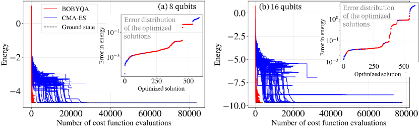
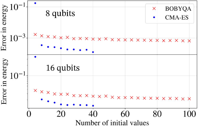
To benchmark different ansaetze, we employ both BOBYQA with 501 random initial values and CMA-ES with 80 random initial values and report the better result from the two methods. Different ansaetze (and different layer numbers) result in vastly different cost-function landscapes and numbers of parameters. A mixed usage of different optimization algorithms, which is widely used in black-box optimization, helps us better navigate through the vast varieties of cost functions. In Fig. 5, we study the noiseless optimization for each optimizer with different initial values. For both eight-qubit and 16-qubit cases, CMA-ES needs more cost function evaluations to converge, as expected for a non-local optimizer. As indicated by the error distribution of the optimized solutions shown in the insets of Fig. 5, some optimization runs with CMA-ES give the best result but others can be far off. The runs also converge to different optimized parameters with the two different optimizers and also different initial values, revealing a complex energy landscape with many local minima. This makes the inclusion of the BOBYQA results helpful, since it allows us to crosscheck the optimizations. A similar conclusion can be made by resampling the distribution shown in the insets of Fig. 5 to investigate the error as a function of the number of initial values of optimization. As shown in Fig. 6, the CMA-ES optimizer gives a better result than BOBYQA after a sufficient number of initial values are used. Hence, BOBYQA serves as a useful cross-check for an insufficient number of initial values. We expect that VQE optimization carried out on QPUs will also benefit from this approach of mixed optimizers with multiple initial values, especially when the QPUs’ clock rate becomes sufficiently high to support a large number of cost function evaluations.
We apply this mixed optimization approach to optimize the three different ansaetze (HVA, HEA-CZ and HEA-XY) with different numbers of layers using a statevector simulator. To make our observation more representative, we run the optimization test with three different setups, namely, four-qubit (GL+), eight-qubit (GL+), 16-qubit (GL+) and eight-qubit (TCz+) (see Table 1 for the parameters values). Except for the simple four-qubit case, the results in Fig. 7 show that the HVA in general outperforms the other two HEAs when a deeper ansatz is used to reduce the error in energy. The main reason for the HEAs’ worse performance is due to the extreme difficulty in the optimization, which is directly related to the barren plateau phenomenon [28]. The number of parameters increases rapidly for HEAs; for example, the four-layer HEA-XY for 16 qubits has 536 parameters. This makes it excessively challenging to scale up the VQE with HEAs to larger circuit depths and system sizes. This is also revealed by the fact that two HEAs show nearly no improvement with increasing number of layers in Fig. 7. Hence, the VQE using HVA will be a more promising approach toward quantum advantage for the square-octagon-lattice Kitaev model.
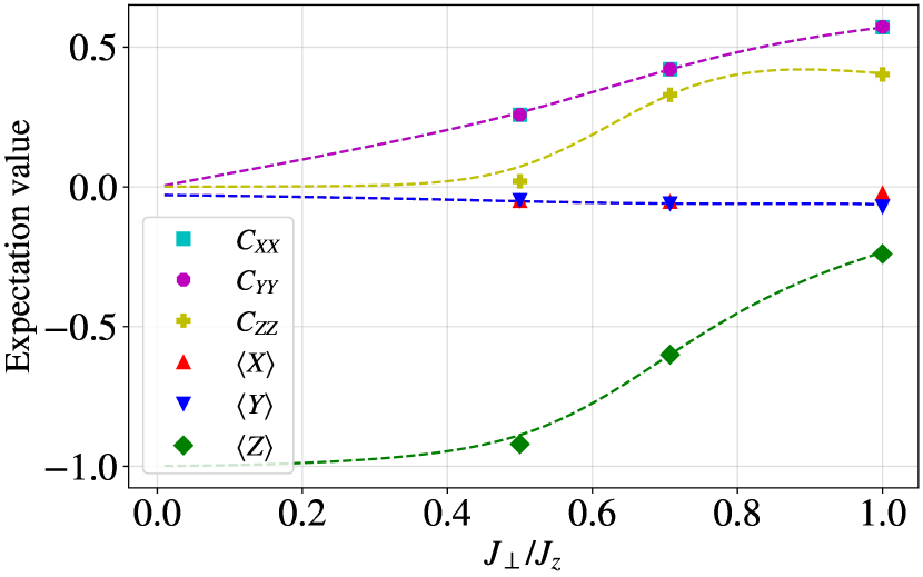
The optimization approach and the HVA ansatz can be used to probe the phase diagram of the model. We demonstrate this potential by determining the single-spin expectation values and static spin-spin correlators in Fig. 8 for an eight-qubit lattice with periodic boundary conditions as shown in Fig. 1(f). We choose this lattice structure and boundary condition so that the system’s behavior is less susceptible to boundary effects. Note that the lattice contains four , , and bonds each. To adapt to this different setup, we have to increase the number of layers of the HVA ansatz to 8 to achieve reasonable accuracy. To characterize the system’s properties as a function of Hamiltonian parameters, we measure the averages of the single-site expectation values , , and over all sites, as well as the averages of the correlators () over all pairs of sites for which . While this small system does not exhibit the exact same phase transitions shown in Fig. 2 for large lattices in the thermodynamic limit, the same set of measurements can be used to study the phase diagram of larger systems. Increasing with a fixed , the eight-qubit lattice shows an increasing average value of while and remain close to zero. Note that the asymmetry between and or at is due to the asymmetry in the lattice geometry. Meanwhile the average correlators all increase gradually from zero as grows. This behavior is captured by the VQE optimization results (data points) as compared to the simulation using ED (dashed lines). One can observe a small deviation between the VQE and ED results for at . This could be improved by increasing the number of layers used with the trade off of higher resource requirements in the optimization.
The phase diagram can also be probed by searching for parameter values where the energy gap between the ground and first excited states closes. By adding the overlap with the ground state to the VQE cost function as discussed in section III.4, we determined the excited-state energies using the same HVA ansatz and optimization approach. For the eight-qubit periodic lattice, we determine the optimal parameters corresponding to the ground states for different values of using the eight-layer HVA ansatz as discussed in the previous paragraph. For excited states, we optimize the modified cost function in eq. 8 with the same eight-layer HVA ansatz. For the optimization, we use CMA-ES with 960 () and 480 () random initial values, and BOBYQA with 6001 () and 3001 () random initial values. We double the number of initial values for as an attempt to improve the accuracy of the excited-state energies determined by the optimization.
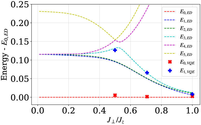
The ground- and excited-state energies determined by VQE are shown in Fig. 9. To better visualize the results, we offset the energy shown in the figure by the ground-state energy determined using ED. We also plot the ED result ( where ) for up to the fifth excited state for comparison. As expected, the VQE results (red crosses) for the ground-state energy are consistent with the ED result (red dashed line) with a small energy error. On the other hand, the excited-state energies (blue pluses) determined by VQE are closest to those of the third excited state instead of the nearly degenerate first and second excited states (except for where the first three excited states are close to each other). This means that while the VQE result still qualitatively predicts the closing of the energy gap, it does not give the correct energy gap between the ground state and the first excited state. We tried multiple values of and observed a similar difficulty in getting to the lower-energy excited states. Future study of alternative ansatz better tailored to the excited states will be needed to improve the accuracy.
| Optimizer | Cost function evaluations | ||
| BFGS, 501 initial values | 0.45069 | 0.42052 | mean: 747, max: 1994 |
| BOBYQA, 501 initial values | 0.27485 | 0.21843 | mean: 471, max: 610 |
| BOBYQA-noisy, 501 initial values | 0.07989 | -0.00453 | mean: 3532, max: 4004 |
| CMA-ES | 0.02416 | -0.06462 | 37570 |
| CMA-ES, 80 initial values | 0.01610 | -0.07125 | mean: 21042, max: 52000 |
| Dual annealing | 0.04534 | -0.01631 | 60101 |
| SPSA | 0.00612 | 0.00879 | 100000 (cutoff) |
IV.2 Simulations with shot noise
It is crucial to take the shot noise into consideration when running variational algorithms on QPUs. If too many measurement shots are requested, the long runtime may be beyond the QPU capacity. If too few shots are requested, the stronger noise may induce undesirable barren plateaus to the cost function landscape [118]. Investigating optimization strategies that tolerate a small number of shots is important for practical applications of the variational algorithms [77].
In this subsection, we evaluate the energy in the simulations with a finite number of shots and then test the optimizers listed in Table 2 once again with the noisy cost function. This allows us to examine the robustness of our optimization approach in the presence of the shot noise. We run the test with 8000 shots using the cost function associated with the four-layer HVA for the eight-qubit lattice and the parameter choice (GL + ) to facilitate the comparison with the noiseless results. The results are summarized in Table 4. To make the effect of the shot noise clear, we determine the energy measured with shot noise and its noiseless counterpart obtained using a statevector simulator for the optimized parameters obtained by minimizing the noisy cost function. The error from the exact ground-state energy shows the performance of the VQE since this quantity is directly related to how close the optimized state is to the ground state. The measured deviation gives us additional information regarding the performance of the optimizers in the presence of the shot noise.
BFGS shows significantly worse performance compared to the noiseless case. The errors introduced by the shot noise are amplified by the small finite step size used by finite-difference methods to compute gradients. The amplified errors make the BFGS much more likely to be trapped. Using analytical methods to determine the gradients directly through measurements [99, 102] could avoid the amplification and would be important when implementing BFGS (and similar gradient-based methods) on QPUs.
The performance of BOBYQA is also worse than that in the noiseless case. This observation is consistent with previous results indicating that BOBYQA typically requires further modifications to optimize the noisy cost function [119]. Here, we adopt one of the simplest modifications to increase the number of interpolation points from to where is the number of parameters. The modified version, BOBYQA-noisy, gives a much improved result as expected. Note that the negative measured deviation suggests that the measured energy associated with the optimized parameters is lower than the exact ground-state energy, which is only possible due to the shot noise. This means that the optimization has converged within the limits set by shot noise. (The standard deviation of 100 energy evaluations with 8000 shots is for all optimized parameters.)
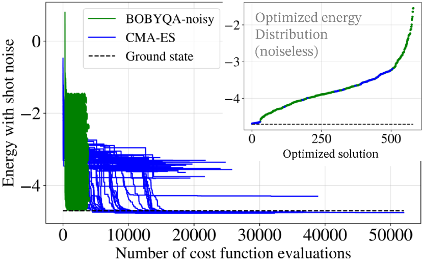
CMA-ES and dual annealing, together with BOBYQA-noisy, have a negative measured deviation for the optimized parameters. (The measured energy is lower than the ground-state energy due to the shot noise.) Among the three optimizers, CMA-ES has the best performance ranked by the error determined by the statevector simulator. Fig. 10 suggests that this superior performance is related to the ability to converge to a better solution by CMA-ES than that by BOBYQA-noisy with the cost of a larger number of cost function evaluations. While CMA-ES may still converge to a poor solution for some initial values, a significant portion of the optimization trajectories converges to solutions close to the ground state. This also suggests the mixed optimization approach is still useful in this noisy case with the BOBYQA-noisy serving as a cross-check of the CMA-ES result.
SPSA shows the best performance among the optimizers being tested. In particular, the error (0.00612) associated with its optimized parameters is even smaller than the noiseless optimization performed by SPSA with an error of 0.04500. This result should not be over-interpreted since these are just two specific optimization trajectories. Nonetheless, this result suggests that the performance of SPSA may be less susceptible to shot noise, and it would be useful to include SPSA to the mixed optimization approach together with other optimizers for VQE with shot noise.
| Qubits | Shots | Error (noiseless) | Measured deviation | Standard deviation of 100 noisy evaluations |
|---|---|---|---|---|
| 8 | 8192 | 0.06977 | -0.00246 | 0.00440 |
| 12 | 4096 | 0.00191 | 0.00406 | 0.00756 |
| 16 | 2048 | 0.14701 | -0.01185 | 0.01103 |
We further explore the performance of SPSA with various magnitudes of shot noise and lattices shown in Fig. 11 with periodic boundary conditions, and SPSA converges within the shot noise limit. QPU experiments are more difficult to be carried out with these lattices since the overhead of SWAP gates to simulate the periodic boundary conditions will be substantial for the existing QPU’s connectivity. Nonetheless, boundary effects on these lattices are less significant compared to those of the lattices with open boundary conditions. It is thus interesting to investigate numerically how the SPSA performs for these lattices. We summarize the results in Table 5 associated with one-layer HVA and the TCz parameter set for the eight-qubit, 12-qubit, and 16-qubit lattices shown in Fig. 11. We decrease the number of shots for larger lattices since sampling is computationally expensive for large lattices. Similarly, to limit the required computational resources, we fix the cutoff of the number of cost function evaluations to be 10000, which is one tenth of that used in the main text. In general, the SPSA optimizer converges to a good solution within the limits set by shot noise. The error of the optimized solution determined using a noiseless statevector simulator spans a much wider range of values for different setups. Further studies with more systematic choices of the number of shots and other lattice and parameter setups will be useful to understand the spread of the errors while SPSA shows a similar level of convergence.
IV.3 QPU experiment
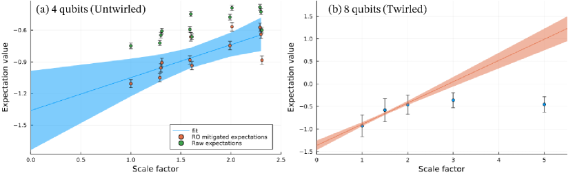
The experimental method has been described in Sec. III.5. As discussed there, we perform a proof-of-concept experiment using the HVA with one layer on four-qubit and eight-qubit sub-lattices of Aspen-9 consisting of qubits , see Fig. 1(b). A schematic HVA-1 circuit for eight qubits is depicted in Fig. 3; in order to execute this on Aspen-9, we identify qubits with qubits , respectively, on Aspen-9. To perform digital ZNE, we increase the total CZ count in the circuit by various scale factors and the expectation values measured at each scale factor are mitigated for readout errors. To improve the results for the eight-qubit case, we twirl the corresponding circuits with random Pauli operators to tailor the noise into a stochastic channel, which may allow ZNE to work better.
Fig. 12 plots the Hamiltonian expectation values in the classically optimized variational state for various scale factors, and the zero-noise limit is extrapolated via Bayesian linear regression. (For the eight-qubit case, the final two scale factors are omitted from the extrapolation because the noise in the system overwhelms any meaningful patterns one could exploit in the extrapolation scheme beyond a scale factor of 2.) The four-qubit experiment gives the extrapolated energy to be which is within one standard deviation of the one-layer-HVA best value and, roughly speaking, the true ground-state energy . The eight-qubit circuit involves more two-qubit gates and a larger infidelity is expected. Anticipating the larger error to be mitigated, we perform randomized compilation or Pauli twirling to improve the performance of ZNE as explained in Sec. III.5. However, even with the additional twirling, we find the extrapolated value for the expectation value to be about (with a standard deviation of about ), which is far from the best value of about that the one-layer HVA can produce in noiseless simulation. This shows that the execution of a -layer HVA circuit for qubits, which contains CZ gates for scale factor , is close to the QPU coherence time. We note that two-qubit gates were executed sequentially in this paper, and parallel execution may lead to an improvement of the results. The relatively large discrepancy between the optimal value obtained on the QPU versus the exact energy suggests the presence of systematic shifts in the gate parameters when they are executed on the QPU. This may be mitigated when performing the optimization entirely on the QPU. Although this is a proof-of-concept experiment, it motivates the use of sophisticated error mitigation techniques along with better gate fidelities to achieve better results on the QPU in the future.
V Conclusion
In this paper, we investigated and benchmarked the appropriate ansatzes and optimization strategies to find the ground state of the square-octagon-lattice Kitaev model with a VQE approach, and demonstrated the ability to determine the system’s properties in different parameter regimes using VQE. We showed that the HVA generally outperforms the two HEAs using CZ or XY gates in the entangling layers. The HEAs require an expensive optimization process due to their rapidly increasing number of parameters with system size and circuit depth, and the unstructured nature of HEAs also makes them susceptible to barren plateaus. The HVA is associated with a relatively easy optimization and is thus better suited to the QPU experiments. The VQE solutions with HVA allow us to probe static expectation values and the energy gap as a function of Hamiltonian parameters, making it possible to probe the phase diagram using VQE. We also conducted an experimental test to run classically optimized four-qubit and eight-qubit HVA circuits on the Aspen-9 QPU. With the help of readout error mitigation and ZNE, the four-qubit experiment gives a result roughly within one standard deviation of the true ground-state energy. For the eight-qubit experiment, the wider and deeper circuit increases the infidelity of the results. There, we observe a substantial difference from the statevector simulation even with the additional randomized compilation. This suggests that extra error mitigation techniques and performing the VQE optimization directly on the QPU would be required to extract useful results from the QPU for the future implementation of Kitaev-model VQE experiments.
Multiple optimization algorithms have been tested to optimize the cost function associated with our VQE application. We find that a mixed usage of different optimizers with multiple initial values gives a much more consistent and better result than just using one specific optimizer with one initial value. In particular, a local optimizer (BOBYQA) mixed with a non-local optimizer (CMA-ES) is shown to be an appropriate strategy for VQE calculations of the Kitaev model. SPSA is also a useful addition to the optimization with shot noise. Although we performed our tests with the noiseless simulator and simulation with shot noise, we expect that QPU experiments will also benefit from this approach as long as the QPU’s clock rate is high enough to support the required number of cost function evaluations.
Acknowledgements.
This material is based upon work supported by the U.S. Department of Energy, Office of Science, National Quantum Information Science Research Centers, Superconducting Quantum Materials and Systems Center (SQMS) under contract number DE-AC02-07CH11359. We would like to thank the entire SQMS algorithms team for fruitful and thought provoking discussions around these works. We would also like to thank the Rigetti team for assistance with running experiments on the Aspen-9 processor, particularly Matt Reagor, Mark Hodson, Bram Evert, Alex Hill, Eric Hulburd and Dylan Anthony. P.P.O. acknowledges useful discussions with Alexander Huynh and Anirban Mukherjee. Some calculations were performed as part of the XSEDE computational Project No. TG-MCA93S030 on Bridges-2 at the Pittsburgh supercomputer center.References
- Childs et al. [2018] A. M. Childs, D. Maslov, Y. Nam, N. J. Ross, and Y. Su, Toward the first quantum simulation with quantum speedup, Proceedings of the National Academy of Sciences 115, 9456 (2018).
- Shor [1995] P. W. Shor, Scheme for reducing decoherence in quantum computer memory, Phys. Rev. A 52, R2493 (1995).
- Roffe [2019] J. Roffe, Quantum error correction: an introductory guide, Contemporary Physics 60, 226 (2019), https://doi.org/10.1080/00107514.2019.1667078 .
- [4] F. Arute, K. Arya, R. Babbush, D. Bacon, J. C. Bardin, R. Barends, A. Bengtsson, S. Boixo, M. Broughton, B. B. Buckley, D. A. Buell, B. Burkett, N. Bushnell, Y. Chen, Z. Chen, Y.-A. Chen, B. Chiaro, R. Collins, S. J. Cotton, W. Courtney, S. Demura, A. Derk, A. Dunsworth, D. Eppens, T. Eckl, C. Erickson, E. Farhi, A. Fowler, B. Foxen, C. Gidney, M. Giustina, R. Graff, J. A. Gross, S. Habegger, M. P. Harrigan, A. Ho, S. Hong, T. Huang, W. Huggins, L. B. Ioffe, S. V. Isakov, E. Jeffrey, Z. Jiang, C. Jones, D. Kafri, K. Kechedzhi, J. Kelly, S. Kim, P. V. Klimov, A. N. Korotkov, F. Kostritsa, D. Landhuis, P. Laptev, M. Lindmark, E. Lucero, M. Marthaler, O. Martin, J. M. Martinis, A. Marusczyk, S. McArdle, J. R. McClean, T. McCourt, M. McEwen, A. Megrant, C. Mejuto-Zaera, X. Mi, M. Mohseni, W. Mruczkiewicz, J. Mutus, O. Naaman, M. Neeley, C. Neill, H. Neven, M. Newman, M. Yuezhen Niu, T. E. O’Brien, E. Ostby, B. Pató, A. Petukhov, H. Putterman, C. Quintana, J.-M. Reiner, P. Roushan, N. C. Rubin, D. Sank, K. J. Satzinger, V. Smelyanskiy, D. Strain, K. J. Sung, P. Schmitteckert, M. Szalay, N. M. Tubman, A. Vainsencher, T. White, N. Vogt, Z. J. Yao, P. Yeh, A. Zalcman, and S. Zanker, Observation of separated dynamics of charge and spin in the Fermi-Hubbard model, arXiv:2010.07965 [quant-ph] .
- Kitaev [2006] A. Kitaev, Anyons in an exactly solved model and beyond, Annals of Physics 321, 2–111 (2006).
- Yang et al. [2007] S. Yang, D. L. Zhou, and C. P. Sun, Mosaic spin models with topological order, Phys. Rev. B 76, 180404(R) (2007).
- Preskill [2018] J. Preskill, Quantum Computing in the NISQ era and beyond, Quantum 2, 79 (2018).
- Cerezo et al. [2021] M. Cerezo, A. Arrasmith, R. Babbush, S. C. Benjamin, S. Endo, K. Fujii, J. R. McClean, K. Mitarai, X. Yuan, L. Cincio, and P. J. Coles, Variational quantum algorithms, Nature Reviews Physics 3, 625 (2021).
- Bharti et al. [2022] K. Bharti, A. Cervera-Lierta, T. H. Kyaw, T. Haug, S. Alperin-Lea, A. Anand, M. Degroote, H. Heimonen, J. S. Kottmann, T. Menke, W.-K. Mok, S. Sim, L.-C. Kwek, and A. Aspuru-Guzik, Noisy intermediate-scale quantum algorithms, Rev. Mod. Phys. 94, 015004 (2022).
- Peruzzo et al. [2014] A. Peruzzo, J. McClean, P. Shadbolt, M.-H. Yung, X.-Q. Zhou, P. J. Love, A. Aspuru-Guzik, and J. L. O’Brien, A variational eigenvalue solver on a photonic quantum processor, Nat. Comm. 5, 1 (2014).
- O’Malley et al. [2016] P. J. J. O’Malley, R. Babbush, I. D. Kivlichan, J. Romero, J. R. McClean, R. Barends, et al., Scalable quantum simulation of molecular energies, Phys. Rev. X 6, 031007 (2016).
- McClean et al. [2016] J. R. McClean, J. Romero, R. Babbush, and A. Aspuru-Guzik, The theory of variational hybrid quantum-classical algorithms, New Journal of Physics 18, 023023 (2016).
- Kandala et al. [2017] A. Kandala, A. Mezzacapo, K. Temme, M. Takita, M. Brink, J. M. Chow, and J. M. Gambetta, Hardware-efficient variational quantum eigensolver for small molecules and quantum magnets, Nature 549, 242 (2017).
- Grimsley et al. [2019] H. R. Grimsley, S. E. Economou, E. Barnes, and N. J. Mayhall, An adaptive variational algorithm for exact molecular simulations on a quantum computer, Nature Communications 10, 3007 (2019).
- Huggins et al. [2020] W. J. Huggins, J. Lee, U. Baek, B. O’Gorman, and K. B. Whaley, A non-orthogonal variational quantum eigensolver, New Journal of Physics 22, 073009 (2020).
- Zhang et al. [2021] F. Zhang, N. Gomes, Y. Yao, P. P. Orth, and T. Iadecola, Adaptive variational quantum eigensolvers for highly excited states, Phys. Rev. B 104, 075159 (2021).
- Tang et al. [2021] H. L. Tang, V. O. Shkolnikov, G. S. Barron, H. R. Grimsley, N. J. Mayhall, E. Barnes, and S. E. Economou, Qubit-ADAPT-VQE: An Adaptive Algorithm for Constructing Hardware-Efficient Ansätze on a Quantum Processor, PRX Quantum 2, 020310 (2021).
- Meitei et al. [2021] O. R. Meitei, B. T. Gard, G. S. Barron, D. P. Pappas, S. E. Economou, E. Barnes, and N. J. Mayhall, Gate-free state preparation for fast variational quantum eigensolver simulations, npj Quantum Information 7, 155 (2021).
- Gomes et al. [2021] N. Gomes, A. Mukherjee, F. Zhang, T. Iadecola, C.-Z. Wang, K.-M. Ho, P. P. Orth, and Y.-X. Yao, Adaptive variational quantum imaginary time evolution approach for ground state preparation, Advanced Quantum Technologies 4, 2100114 (2021).
- Van Dyke et al. [2022] J. S. Van Dyke, G. S. Barron, N. J. Mayhall, E. Barnes, and S. E. Economou, Scaling adaptive quantum simulation algorithms via operator pool tiling, arXiv:2206.14215 10.48550/ARXIV.2206.14215 (2022).
- Mukherjee et al. [2023] A. Mukherjee, N. F. Berthusen, J. C. Getelina, P. P. Orth, and Y.-X. Yao, Comparative study of adaptive variational quantum eigensolvers for multi-orbital impurity models, Communications Physics 6, 4 (2023).
- Anastasiou et al. [2022] P. G. Anastasiou, Y. Chen, N. J. Mayhall, E. Barnes, and S. E. Economou, TETRIS-ADAPT-VQE: An adaptive algorithm that yields shallower, denser circuit ansätze, arXiv:2209.10562 10.48550/ARXIV.2209.10562 (2022).
- Zhang et al. [2022a] Y. Zhang, L. Cincio, C. F. A. Negre, P. Czarnik, P. J. Coles, P. M. Anisimov, S. M. Mniszewski, S. Tretiak, and P. A. Dub, Variational quantum eigensolver with reduced circuit complexity, npj Quantum Information 8, 96 (2022a).
- Wecker et al. [2015] D. Wecker, M. B. Hastings, and M. Troyer, Progress towards practical quantum variational algorithms, Phys. Rev. A 92, 042303 (2015).
- Farhi et al. [2000] E. Farhi, J. Goldstone, S. Gutmann, and M. Sipser, Quantum computation by adiabatic evolution, arXiv preprint quant-ph/0001106 (2000).
- Farhi et al. [2014] E. Farhi, J. Goldstone, and S. Gutmann, A quantum approximate optimization algorithm (2014), arXiv:1411.4028 [quant-ph] .
- Wiersema et al. [2020] R. Wiersema, C. Zhou, Y. de Sereville, J. F. Carrasquilla, Y. B. Kim, and H. Yuen, Exploring entanglement and optimization within the Hamiltonian Variational Ansatz, PRX Quantum 1, 020319 (2020).
- McClean et al. [2018] J. R. McClean, S. Boixo, V. N. Smelyanskiy, R. Babbush, and H. Neven, Barren plateaus in quantum neural network training landscapes, Nat. Commun. 9, 4812 (2018).
- Larocca et al. [2022] M. Larocca, P. Czarnik, K. Sharma, G. Muraleedharan, P. J. Coles, and M. Cerezo, Diagnosing Barren plateaus with tools from quantum optimal control, Quantum 6, 824 (2022).
- Hermanns et al. [2018] M. Hermanns, I. Kimchi, and J. Knolle, Physics of the Kitaev model: Fractionalization, dynamic correlations, and material connections, Annual Review of Condensed Matter Physics 9, 17 (2018).
- Takagi et al. [2019] H. Takagi, T. Takayama, G. Jackeli, G. Khaliullin, and S. E. Nagler, Concept and realization of Kitaev quantum spin liquids, Nature Reviews Physics 1, 264 (2019).
- Hickey and Trebst [2019] C. Hickey and S. Trebst, Emergence of a field-driven u(1) spin liquid in the Kitaev honeycomb model, Nature Communications 10, 530 (2019).
- Nayak et al. [2008] C. Nayak, S. H. Simon, A. Stern, M. Freedman, and S. Das Sarma, Non-Abelian anyons and topological quantum computation, Rev. Mod. Phys. 80, 1083 (2008).
- Lee et al. [2017] Y.-C. Lee, C. G. Brell, and S. T. Flammia, Topological quantum error correction in the Kitaev honeycomb model, Journal of Statistical Mechanics: Theory and Experiment 2017, 083106 (2017).
- Freedman et al. [2002] M. H. Freedman, M. Larsen, and Z. Wang, A modular functor which is universal¶for quantum computation, Communications in Mathematical Physics 227, 605 (2002).
- Jackeli and Khaliullin [2009] G. Jackeli and G. Khaliullin, Mott insulators in the strong spin-orbit coupling limit: From Heisenberg to a quantum compass and Kitaev models, Phys. Rev. Lett. 102, 017205 (2009).
- Banerjee et al. [2016] A. Banerjee, C. A. Bridges, J.-Q. Yan, A. A. Aczel, L. Li, M. B. Stone, G. E. Granroth, M. D. Lumsden, Y. Yiu, J. Knolle, and et al., Proximate Kitaev quantum spin liquid behaviour in a honeycomb magnet, Nature Materials 15, 733–740 (2016).
- Banerjee et al. [2018] A. Banerjee, P. Lampen-Kelley, J. Knolle, C. Balz, A. A. Aczel, B. Winn, Y. Liu, D. Pajerowski, J. Yan, C. A. Bridges, and et al., Excitations in the field-induced quantum spin liquid state of -RuCl3, npj Quantum Materials 3, 8 (2018).
- Kasahara et al. [2018] Y. Kasahara, K. Sugii, T. Ohnishi, M. Shimozawa, M. Yamashita, N. Kurita, H. Tanaka, J. Nasu, Y. Motome, T. Shibauchi, et al., Unusual thermal Hall effect in a Kitaev spin liquid candidate - RuCl 3, Physical review letters 120, 217205 (2018).
- Yokoi et al. [2021] T. Yokoi, S. Ma, Y. Kasahara, S. Kasahara, T. Shibauchi, N. Kurita, H. Tanaka, J. Nasu, Y. Motome, C. Hickey, S. Trebst, and Y. Matsuda, Half-integer quantized anomalous thermal hall effect in the kitaev material candidate -RuCl3, Science 373, 568 (2021).
- Chaloupka et al. [2010] J. Chaloupka, G. Jackeli, and G. Khaliullin, Kitaev-Heisenberg model on a honeycomb lattice: Possible exotic phases in Iridium oxides , Phys. Rev. Lett. 105, 027204 (2010).
- Jiang et al. [2011] H.-C. Jiang, Z.-C. Gu, X.-L. Qi, and S. Trebst, Possible proximity of the Mott insulating iridate Na2IrO3 to a topological phase: Phase diagram of the Heisenberg-Kitaev model in a magnetic field, Phys. Rev. B 83, 245104 (2011).
- Chaloupka et al. [2013] J. Chaloupka, G. Jackeli, and G. Khaliullin, Zigzag magnetic order in the Iridium oxide , Phys. Rev. Lett. 110, 097204 (2013).
- Osorio Iregui et al. [2014] J. Osorio Iregui, P. Corboz, and M. Troyer, Probing the stability of the spin-liquid phases in the Kitaev-Heisenberg model using tensor network algorithms, Phys. Rev. B 90, 195102 (2014).
- Rau et al. [2014] J. G. Rau, E. K.-H. Lee, and H.-Y. Kee, Generic spin model for the honeycomb iridates beyond the Kitaev limit, Phys. Rev. Lett. 112, 077204 (2014).
- Shinjo et al. [2015] K. Shinjo, S. Sota, and T. Tohyama, Density-matrix renormalization group study of the extended Kitaev-Heisenberg model, Phys. Rev. B 91, 054401 (2015).
- Winter et al. [2016] S. M. Winter, Y. Li, H. O. Jeschke, and R. Valentí, Challenges in design of Kitaev materials: Magnetic interactions from competing energy scales, Phys. Rev. B 93, 214431 (2016).
- Yadav et al. [2016] R. Yadav, N. A. Bogdanov, V. M. Katukuri, S. Nishimoto, J. Van Den Brink, and L. Hozoi, Kitaev exchange and field-induced quantum spin-liquid states in honeycomb -RuCl 3, Scientific reports 6, 1 (2016).
- Gohlke et al. [2017] M. Gohlke, R. Verresen, R. Moessner, and F. Pollmann, Dynamics of the Kitaev-Heisenberg model, Phys. Rev. Lett. 119, 157203 (2017).
- Gotfryd et al. [2017] D. Gotfryd, J. Rusnačko, K. Wohlfeld, G. Jackeli, J. c. v. Chaloupka, and A. M. Oleś, Phase diagram and spin correlations of the Kitaev-Heisenberg model: Importance of quantum effects, Phys. Rev. B 95, 024426 (2017).
- Zhu et al. [2018] Z. Zhu, I. Kimchi, D. N. Sheng, and L. Fu, Robust non-Abelian spin liquid and a possible intermediate phase in the antiferromagnetic Kitaev model with magnetic field, Phys. Rev. B 97, 241110(R) (2018).
- Patel and Trivedi [2019] N. D. Patel and N. Trivedi, Magnetic field-induced intermediate quantum spin liquid with a spinon fermi surface, Proceedings of the National Academy of Sciences 116, 12199 (2019).
- Gordon et al. [2019] J. S. Gordon, A. Catuneanu, E. S. Sørensen, and H.-Y. Kee, Theory of the field-revealed Kitaev spin liquid, Nature communications 10, 1 (2019).
- Czarnik et al. [2019] P. Czarnik, A. Francuz, and J. Dziarmaga, Tensor network simulation of the Kitaev-Heisenberg model at finite temperature, Physical Review B 100, 165147 (2019).
- Lee et al. [2020] H.-Y. Lee, R. Kaneko, L. E. Chern, T. Okubo, Y. Yamaji, N. Kawashima, and Y. B. Kim, Magnetic field induced quantum phases in a tensor network study of Kitaev magnets, Nature communications 11, 1 (2020).
- White [1992] S. R. White, Density matrix formulation for quantum renormalization groups, Phys. Rev. Lett. 69, 2863 (1992).
- Schollwöck [2011] U. Schollwöck, The density-matrix renormalization group in the age of matrix product states, Annals of Physics 326, 96–192 (2011).
- Fishman et al. [2022] M. Fishman, S. R. White, and E. M. Stoudenmire, The ITensor software library for tensor network calculations, SciPost Phys. Codebases , 4 (2022).
- Mishchenko et al. [2021] P. A. Mishchenko, Y. Kato, and Y. Motome, Quantum Monte Carlo method on asymptotic Lefschetz thimbles for quantum spin systems: An application to the Kitaev model in a magnetic field, Phys. Rev. D 104, 074517 (2021).
- Kurita et al. [2015] M. Kurita, Y. Yamaji, S. Morita, and M. Imada, Variational Monte Carlo method in the presence of spin-orbit interaction and its application to Kitaev and Kitaev-Heisenberg models, Phys. Rev. B 92, 035122 (2015).
- Kells et al. [2011] G. Kells, J. Kailasvuori, J. K. Slingerland, and J. Vala, Kaleidoscope of topological phases with multiple majorana species, New Journal of Physics 13, 095014 (2011).
- Hong et al. [2020] S. S. Hong, A. T. Papageorge, P. Sivarajah, G. Crossman, N. Didier, A. M. Polloreno, E. A. Sete, S. W. Turkowski, M. P. da Silva, and B. R. Johnson, Demonstration of a parametrically activated entangling gate protected from flux noise, Phys. Rev. A 101, 012302 (2020).
- Abrams et al. [2020] D. M. Abrams, N. Didier, M. P. Johnson, Blake R .and da Silva, and C. A. Ryan, Implementation of XY entangling gates with a single calibrated pulse, Nature Electronics 3, 744 (2020).
- Reagor et al. [2018] M. Reagor et al., Demonstration of universal parametric entangling gates on a multi-qubit lattice, Sci. Adv. 4, eaao3603 (2018).
- Berke et al. [2020] C. Berke, S. Trebst, and C. Hickey, Field stability of majorana spin liquids in antiferromagnetic Kitaev models, Phys. Rev. B 101, 214442 (2020).
- Hickey et al. [2021] C. Hickey, M. Gohlke, C. Berke, and S. Trebst, Generic field-driven phenomena in Kitaev spin liquids: Canted magnetism and proximate spin liquid physics, Phys. Rev. B 103, 064417 (2021).
- Yamada [2021] M. G. Yamada, Topological invariant in Kitaev spin liquids: Classification of gapped spin liquids beyond projective symmetry group, Phys. Rev. Research 3, L012001 (2021).
- Bespalova and Kyriienko [2021] T. A. Bespalova and O. Kyriienko, Quantum simulation and ground state preparation for the honeycomb Kitaev model (2021), arXiv:2109.13883 [quant-ph] .
- Jahin et al. [2022] A. Jahin, A. C. Y. Li, T. Iadecola, P. P. Orth, G. N. Perdue, A. Macridin, M. S. Alam, and N. M. Tubman, Fermionic approach to variational quantum simulation of Kitaev spin models, Phys. Rev. A 106, 022434 (2022).
- Kitaev [2003] A. Kitaev, Fault-tolerant quantum computation by anyons, Annals of Physics 303, 2–30 (2003).
- Wen [2003] X.-G. Wen, Quantum orders in an exact soluble model, Phys. Rev. Lett. 90, 016803 (2003).
- Nussinov and Ortiz [2009] Z. Nussinov and G. Ortiz, A symmetry principle for topological quantum order, Annals of Physics 324, 977–1057 (2009).
- Brown et al. [2011] B. J. Brown, W. Son, C. V. Kraus, R. Fazio, and V. Vedral, Generating topological order from a two-dimensional cluster state using a duality mapping, New Journal of Physics 13, 065010 (2011).
- Zhang et al. [2022b] D.-B. Zhang, B.-L. Chen, Z.-H. Yuan, and T. Yin, Variational quantum eigensolvers by variance minimization, Chinese Physics B 31, 120301 (2022b).
- Nakanishi et al. [2019] K. M. Nakanishi, K. Mitarai, and K. Fujii, Subspace-search variational quantum eigensolver for excited states, Phys. Rev. Research 1, 033062 (2019).
- Higgott et al. [2019] O. Higgott, D. Wang, and S. Brierley, Variational Quantum Computation of Excited States, Quantum 3, 156 (2019).
- Gu et al. [2021] A. Gu, A. Lowe, P. A. Dub, P. J. Coles, and A. Arrasmith, Adaptive shot allocation for fast convergence in variational quantum algorithms, arXiv e-prints , arXiv:2108.10434 (2021), arXiv:2108.10434 [quant-ph] .
- Ho and Hsieh [2019] W. W. Ho and T. H. Hsieh, Efficient variational simulation of non-trivial quantum states, SciPost Phys. 6, 29 (2019).
- Cade et al. [2020] C. Cade, L. Mineh, A. Montanaro, and S. Stanisic, Strategies for solving the Fermi-Hubbard model on near-term quantum computers, Phys. Rev. B 102, 235122 (2020).
- Lavrijsen et al. [2020] W. Lavrijsen, A. Tudor, J. Müller, C. Iancu, and W. de Jong, Classical optimizers for noisy intermediate-scale quantum devices, in 2020 IEEE International Conference on Quantum Computing and Engineering (QCE) (2020) pp. 267–277.
- Anand et al. [2021] A. Anand, M. Degroote, and A. Aspuru-Guzik, Natural evolutionary strategies for variational quantum computation, Machine Learning: Science and Technology 2, 045012 (2021).
- Harrow and Napp [2021] A. W. Harrow and J. C. Napp, Low-depth gradient measurements can improve convergence in variational hybrid quantum-classical algorithms, Phys. Rev. Lett. 126, 140502 (2021).
- Smith et al. [2016] R. S. Smith, M. J. Curtis, and W. J. Zeng, A Practical Quantum Instruction Set Architecture, arXiv e-prints , arXiv:1608.03355 (2016), arXiv:1608.03355 [quant-ph] .
- Cirq Developers [2022] Cirq Developers, Cirq (2022), See full list of authors on Github: https://github .com/quantumlib/Cirq/graphs/contributors.
- Qiskit contributors [2023] Qiskit contributors, Qiskit: An open-source framework for quantum computing (2023).
- Havlíček et al. [2019] V. Havlíček, A. D. Córcoles, K. Temme, A. W. Harrow, A. Kandala, J. M. Chow, and J. M. Gambetta, Supervised learning with quantum-enhanced feature spaces, Nature 567, 209 (2019).
- Peters et al. [2021] E. Peters, J. Caldeira, A. Ho, S. Leichenauer, M. Mohseni, H. Neven, P. Spentzouris, D. Strain, and G. N. Perdue, Machine learning of high dimensional data on a noisy quantum processor, npj Quantum Information 7, 161 (2021).
- Smith et al. [2020] R. S. Smith, E. C. Peterson, M. G. Skilbeck, and E. J. Davis, An open-source, industrial-strength optimizing compiler for quantum programs, Quantum Science and Technology 5, 044001 (2020), arXiv:2003.13961 [quant-ph] .
- Karalekas et al. [2020] P. J. Karalekas, N. A. Tezak, E. C. Peterson, C. A. Ryan, M. P. da Silva, and R. S. Smith, A quantum-classical cloud platform optimized for variational hybrid algorithms, Quantum Science and Technology 5, 024003 (2020).
- Virtanen et al. [2020] P. Virtanen, R. Gommers, T. E. Oliphant, M. Haberland, T. Reddy, D. Cournapeau, E. Burovski, P. Peterson, W. Weckesser, J. Bright, S. J. van der Walt, M. Brett, J. Wilson, K. J. Millman, N. Mayorov, A. R. J. Nelson, E. Jones, R. Kern, E. Larson, C. J. Carey, İ. Polat, Y. Feng, E. W. Moore, J. VanderPlas, D. Laxalde, J. Perktold, R. Cimrman, I. Henriksen, E. A. Quintero, C. R. Harris, A. M. Archibald, A. H. Ribeiro, F. Pedregosa, P. van Mulbregt, and SciPy 1.0 Contributors, SciPy 1.0: Fundamental Algorithms for Scientific Computing in Python, Nature Methods 17, 261 (2020).
- Powell [2009] M. J. D. Powell, The BOBYQA algorithm for bound constrained optimization without derivatives, Cambridge NA Report NA2009/06 , 26 (2009).
- [92] Michael J. D. Powell, Bobyqa.
- Hansen et al. [2019] N. Hansen, Y. Akimoto, and P. Baudis, CMA-ES/pycma on Github, Zenodo, DOI:10.5281/zenodo.2559634 (2019).
- Gomez-Dans [2012] J. Gomez-Dans, Spsa, https://github.com/jgomezdans/spsa (2012).
- Hansen and Ostermeier [2001] N. Hansen and A. Ostermeier, Completely derandomized self-adaptation in evolution strategies, Evol. Comput. 9, 159 (2001).
- Xiang et al. [1997] Y. Xiang, D. Sun, W. Fan, and X. Gong, Generalized simulated annealing algorithm and its application to the Thomson model, Physics Letters A 233, 216 (1997).
- Spall [1992] J. C. Spall, Multivariate stochastic approximation using a simultaneous perturbation gradient approximation, IEEE Trans. Automat. Contr. 37, 332 (1992).
- Rios and Sahinidis [2013] L. M. Rios and N. V. Sahinidis, Derivative-free optimization: a review of algorithms and comparison of software implementations, J. Global Optim. 56, 1247 (2013).
- Romero et al. [2018] J. Romero, R. Babbush, J. R. McClean, C. Hempel, P. J. Love, and A. Aspuru-Guzik, Strategies for quantum computing molecular energies using the unitary coupled cluster ansatz, Quantum Science and Technology 4, 014008 (2018).
- Gilyén et al. [2019] A. Gilyén, S. Arunachalam, and N. Wiebe, Optimizing quantum optimization algorithms via faster quantum gradient computation, in Proceedings of the 2019 Annual ACM-SIAM Symposium on Discrete Algorithms (SODA) (2019) pp. 1425–1444.
- Schuld et al. [2019] M. Schuld, V. Bergholm, C. Gogolin, J. Izaac, and N. Killoran, Evaluating analytic gradients on quantum hardware, Phys. Rev. A 99, 032331 (2019).
- Mitarai et al. [2020] K. Mitarai, Y. O. Nakagawa, and W. Mizukami, Theory of analytical energy derivatives for the variational quantum eigensolver, Phys. Rev. Research 2, 013129 (2020).
- Izmaylov et al. [2021] A. F. Izmaylov, R. A. Lang, and T.-C. Yen, Analytic gradients in variational quantum algorithms: Algebraic extensions of the parameter-shift rule to general unitary transformations, Phys. Rev. A 104, 062443 (2021).
- Huggins et al. [2022] W. J. Huggins, B. A. O’Gorman, N. C. Rubin, D. R. Reichman, R. Babbush, and J. Lee, Unbiasing fermionic quantum Monte Carlo with a quantum computer, Nature 603, 416 (2022).
- Klymko et al. [2022] K. Klymko, C. Mejuto-Zaera, S. J. Cotton, F. Wudarski, M. Urbanek, D. Hait, M. Head-Gordon, K. B. Whaley, J. Moussa, N. Wiebe, W. A. de Jong, and N. M. Tubman, Real-time evolution for ultracompact Hamiltonian eigenstates on quantum hardware, PRX Quantum 3, 020323 (2022).
- Li and Benjamin [2017] Y. Li and S. C. Benjamin, Efficient variational quantum simulator incorporating active error minimization, Phys. Rev. X 7, 021050 (2017).
- Temme et al. [2017] K. Temme, S. Bravyi, and J. M. Gambetta, Error mitigation for short-depth quantum circuits, Phys. Rev. Lett. 119, 180509 (2017).
- Giurgica-Tiron et al. [2020] T. Giurgica-Tiron, Y. Hindy, R. LaRose, A. Mari, and W. J. Zeng, Digital zero noise extrapolation for quantum error mitigation, in 2020 IEEE International Conference on Quantum Computing and Engineering (QCE) (2020) pp. 306–316.
- Geller [2020] M. R. Geller, Rigorous measurement error correction, Quantum Sci. Technol. 5, 03LT01 (2020).
- Wallman and Emerson [2016] J. J. Wallman and J. Emerson, Noise tailoring for scalable quantum computation via randomized compiling, Phys. Rev. A 94, 052325 (2016).
- Note [1] Note that the same unitary can also be written , so that the CZ gate remains invariant if we swap the labels and . Therefore, it doesn’t matter how we assign the labels control/target to the two qubits participating in this interaction.
- Schultz et al. [2022] K. Schultz, R. LaRose, A. Mari, G. Quiroz, N. Shammah, B. D. Clader, and W. J. Zeng, Impact of time-correlated noise on zero-noise extrapolation, Phys. Rev. A 106, 052406 (2022).
- Cai et al. [2022] Z. Cai, R. Babbush, S. C. Benjamin, S. Endo, W. J. Huggins, Y. Li, J. R. McClean, and T. E. O’Brien, Quantum error mitigation, arXiv:2210.00921 10.48550/ARXIV.2210.00921 (2022).
- Russo et al. [2022] V. Russo, A. Mari, N. Shammah, R. LaRose, and W. J. Zeng, Testing platform-independent quantum error mitigation on noisy quantum computers, arXiv:2210.07194 10.48550/ARXIV.2210.07194 (2022).
- Ge et al. [2018] H. Ge, K. Xu, and Z. Ghahramani, Turing: a language for flexible probabilistic inference, in International Conference on Artificial Intelligence and Statistics, AISTATS 2018, 9-11 April 2018, Playa Blanca, Lanzarote, Canary Islands, Spain (2018) pp. 1682–1690.
- Hoffman et al. [2014] M. D. Hoffman, A. Gelman, et al., The no-u-turn sampler: adaptively setting path lengths in hamiltonian Monte Carlo., J. Mach. Learn. Res. 15, 1593 (2014).
- Rubin [1981] D. B. Rubin, The bayesian bootstrap, The annals of statistics , 130 (1981).
- Wang et al. [2021] S. Wang, E. Fontana, M. Cerezo, K. Sharma, A. Sone, L. Cincio, and P. J. Coles, Noise-induced barren plateaus in variational quantum algorithms, Nature communications 12, 6961 (2021).
- Cartis et al. [2019] C. Cartis, J. Fiala, B. Marteau, and L. Roberts, Improving the flexibility and robustness of model-based derivative-free optimization solvers, ACM Trans. Math. Softw. 45, 10.1145/3338517 (2019).