Trace decreasing quantum dynamical maps: Divisibility and entanglement dynamics

Abstract

Trace decreasing quantum operations naturally emerge in experiments involving postselection. However, the experiments usually focus on dynamics of the conditional output states as if the dynamics were trace preserving. Here we show that this approach leads to incorrect conclusions about the dynamics divisibility, namely, one can observe an increase in the trace distance or the system-ancilla entanglement although the trace decreasing dynamics is completely positive divisible. We propose solutions to that problem and introduce proper indicators of the information backflow and the indivisibility. We also review a recently introduced concept of the generalized erasure dynamics that includes more experimental data in the dynamics description. The ideas are illustrated by explicit physical examples of polarization dependent losses.

1 Introduction

Many quantum physics experiments involve a postselection, i.e., an analysis of only those events that are conditioned by some measurement outcomes. Examples include the approximate preparation of a single-photon state via detecting a heralding photon in the parametric down-conversion process [1], the implementation of the conditional quantum gates [2], the generation of high-dimensional maximally entangled orbital-angular-momentum states [3], the conditional subtraction of a single photon [4] or multiple photons [5] from the electromagnetic field, the conditional addition of a single photon to the electromagnetic field [6], the experimental evaluation of so-called weak values [7], and the simulation of quantum collision models [8]. A proper mathematical description of any postselection procedure is given by a quantum operation, i.e., a trace nonincreasing completely positive map $\Lambda$ (see, e.g., [9]) that is associated with a specific measurement outcome. If $\varrho$ is an initial density operator before postselection, then $\Lambda[\varrho]$ is a subnormalized density operator such that the trace ${\rm tr}\big{[}\Lambda[\varrho]\big{]}$ is exactly the probability to get that specific measurement outcome.

In general, a measurement-induced transformation of the system state is fully described in terms of the quantum instrument that assigns a quantum operation to each measurement outcome [10, 11, 12]. A quantum operation $\Lambda$ corresponds to a specific measurement outcome, say, a successful detection of the heralding photon in quantum optics experiments [1, 2, 4, 6]. In mathematical description of experiments with photon subtraction or photon addition [4, 6], however, the conventionally used transformations $\varrho\rightarrow ta\varrho a^{{\dagger}}$ and $\varrho\rightarrow ta^{{\dagger}}\varrho a$ are not legitimate quantum operations for any constant $t>0$ due to the violation of the trace nonincreasing property [13] ($a$ and $a^{{\dagger}}$ are the photon annihilation operator and the photon creation operator for a considered mode, respectively). The transformations above approximate the faithful quantum operations of photon substraction and addition for density operators from some class [13].

To illustrate a simple trace nonincreasing operation, let us consider an experiment with polarization qubits. Suppose $\varrho$ is a density operator for polarization degrees of freedom of single photons and those single photons propagate through a lossy optical fiber with the intensity attenuation factor $p$, then $\Lambda[\varrho]=p\varrho$ and ${\rm tr}\big{[}\Lambda[\varrho]\big{]}=p$. The attenuation factor is experimentally estimated as $N_{\rm out}/N_{\rm in}$, where $N_{\rm out}$ is the number of photons detected at the output of the fiber and $N_{\rm in}$ is the number of photons that enter the fiber. If the photon detector has a finite quantum efficiency $\eta$, then the number of successfully detected photons at the input (the output) of the fiber approximately equals $N_{\rm in}^{\prime}=\eta N_{\rm in}$ ($N_{\rm out}^{\prime}=\eta N_{\rm out}$) so that $N_{\rm out}^{\prime}/N_{\rm in}^{\prime}=N_{\rm out}/N_{\rm in}$, i.e., ${\rm tr}\big{[}\Lambda[\varrho]\big{]}$ can be correctly estimated even with the use of imperfect devices. Alternatively, the photon pairs can be produced in the parametric down-conversion process, with one photon being sent to a lossy channel (to count $N_{\rm out}^{\prime}$ at the output) and the other one being used as a herald (to count $N_{\rm in}^{\prime}$). These ideas enable one to reconstruct a trace nonincreasing operation based on experimental data. For instance, the experimental quantum process tomography of a trace decreasing map $\Lambda$ describing the partially transmitting polarizing beam splitter is reported in Ref. [14].

The whole idea of postselection is focused on the conditional output state

$$\varrho_{\rm out}=\frac{\Lambda[\varrho]}{{\rm tr}\big{[}\Lambda[\varrho]\big{]}}\equiv\Lambda_{{\cal D}}[\varrho]$$

that is a valid density operator provided ${\rm tr}\big{[}\Lambda[\varrho]\big{]}>0$. (If ${\rm tr}\big{[}\Lambda[\varrho]\big{]}=0$, then there is no sense in postselection because a desired measurement outcome is never observed.) The introduced map $\Lambda_{{\cal D}}$ defines a nonlinear transformation of density operators that finds applications in the stroboscopic implementation of effective non-Hermitian Hamiltonians [15, 16]. In this work, we are primarily interested in biased operations $\Lambda$ that have the property ${\rm tr}\big{[}\Lambda[\varrho_{1}]\big{]}\neq{\rm tr}\big{[}\Lambda[\varrho_{2}]\big{]}$ for at least two density operators $\varrho_{1}$ and $\varrho_{2}$ [17]. Examples of biased quantum operations include the partially transmitting polarizing beam splitter [14] and the polarization-dependent losses [18].

Interestingly, the optical simulator of quantum collisions [8] produces a sequence of quantum operations $\Lambda(t_{m})$ in the single-photon sector that correspond to transformations from time $t=0$ to a number of different time moments $t=t_{m}$, $m=1,2,\ldots$. Similarly, one can consider losses in optical fibers of different length to get a one-parameter family of quantum operations $\{\Lambda(t)\}_{t\geq 0}$ that we refer to as a trace decreasing dynamical map if ${\rm tr}\big{[}\Lambda(t)[\varrho]\big{]}<1$ for some density operator $\varrho$ and some $t\geq 0$. Note that the relation ${\rm tr}\big{[}\Lambda(t_{1})[\varrho]\big{]}\geq{\rm tr}\big{[}\Lambda(t_{2})[\varrho]\big{]}$ for $t_{2}\geq t_{1}\geq 0$ need not hold in general. Suppose $\Lambda(t_{2})=\Theta(t_{2},t_{1})\Lambda(t_{1})$ for all $t_{2}\geq t_{1}\geq 0$, where $\Theta(t_{2},t_{1})$ is a legitimate quantum operation (i.e., a completely positive and trace nonincreasing map). Then $\Lambda(t)$ is called completely positive divisible (CP-divisible). Physical meaning of CP-divisibility is that the dynamics $\Lambda(t)$ can be effectively viewed as a concatenation of independent subevolutions.

As far as trace preserving dynamical maps $\{\Phi(t)\}_{t\geq 0}$ are concerned, CP-divisibility is studied in a number of papers and many different indicators of CP-indivisibility are proposed too (see, e.g., [19, 20, 21, 22, 23, 24]). However, in the following Secs. we show that these indicators become misleading if carelessly applied to postselected states of a trace decreasing dynamical map $\{\Lambda(t)\}_{t\geq 0}$. Note that some authors associate CP-divisibility with a quantum version of the Markovian process [19]; however, a more complicated relation takes place operationally [25].

2 Trace distance approach to non-Markovianity

Let $\varrho_{1}$ and $\varrho_{2}$ be density operators, then the trace distance $\frac{1}{2}\|\Phi(t)[\varrho_{1}]-\Phi(t)[\varrho_{2}]\|_{1}$ is a nonincreasing function of time $t$ if the trace preserving dynamical map $\{\Phi(t)\}_{t\geq 0}$ is CP-divisible [24]. The physical meaning of the trace distance is related with the maximum success probability to distinguish the initially equiprobable states $\varrho_{1}$ and $\varrho_{2}$ after time $t$. The maximum success probability equals $\frac{1}{2}+\frac{1}{4}\|\Phi(t)[\varrho_{1}]-\Phi(t)[\varrho_{2}]\|_{1}$ in this case (see, e.g., [12]). If the trace distance diminishes, then the success probability diminishes too, which is treated as a flow of information from the open system to its environment. On the other hand, the increase of the trace distance is an indication of the backflow of information according to Ref. [24].

If one experimentally reconstructs the conditional output states $\Lambda_{\cal D}(t)[\varrho_{1}]=\Lambda(t)[\varrho_{1}]/{\rm tr}\big{[}\Lambda(t)[\varrho_{1}]\big{]}$ and $\Lambda_{\cal D}(t)[\varrho_{2}]=\Lambda(t)[\varrho_{2}]/{\rm tr}\big{[}\Lambda(t)[\varrho_{2}]\big{]}$, then it is tempting to use the conventional trace distance

$$\frac{1}{2}\|\Lambda_{\cal D}(t)[\varrho_{1}]-\Lambda_{\cal D}(t)[\varrho_{2}]\|_{1}$$ (1)

to analyze the information flow. However, this approach encounters a number of problems. First, the probabilities $p_{1}(t):={\rm tr}\big{[}\Lambda(t)[\varrho_{1}]\big{]}$ and $p_{2}(t):={\rm tr}\big{[}\Lambda(t)[\varrho_{2}]\big{]}$ differ in general. This means that by using Eq. (1) an experimentalist disregards some extra information on how often the states $\Lambda_{\cal D}(t)[\varrho_{1}]$ and $\Lambda_{\cal D}(t)[\varrho_{2}]$ are actually produced. Second, as we show in the example below, the quantity (1) may increase even for a semigroup trace decreasing dynamics $\Lambda(t)$ that is obviously CP-divisible.

Example 2.1.

Consider the polarization qubit dynamics $\Lambda(t)=e^{Lt}$, where

$$L[\varrho]=-\frac{1}{2}\Big{\{}\gamma_{H}\ket{H}\bra{H}+\gamma_{V}\ket{V}\bra{V},\varrho\Big{\}},$$ (2)

$\{\cdot,\cdot\}$ stands for the anticommutator; $(\ket{H},\ket{V})$ is a conventional basis composed of the horizontally and vertically polarized states; $\gamma_{H}$ and $\gamma_{V}$ are the attenuation rates for horizontally and vertically polarized photons, respectively. Suppose $\varrho_{1}=\ket{H}\bra{H}$ and $\varrho_{2}=\frac{1}{2}(\ket{H}+\ket{V})(\bra{H}+\bra{V})$, then we explicitly find the subnormalized states in the basis $(\ket{H},\ket{V})$,

$$\Lambda(t)[\varrho_{1}]=\left(\begin{array}[]{cc}e^{-\gamma_{H}t}&0\\ 0&0\\ \end{array}\right),\quad\Lambda(t)[\varrho_{2}]=\frac{1}{2}\left(\begin{array}[]{cc}e^{-\gamma_{H}t}&e^{-(\gamma_{H}+\gamma_{V})t/2}\\ e^{-(\gamma_{H}+\gamma_{V})t/2}&e^{-\gamma_{V}t}\\ \end{array}\right),$$

and the corresponding conditional output states,

$$\Lambda_{\cal D}(t)[\varrho_{1}]=\left(\begin{array}[]{cc}1&0\\ 0&0\\ \end{array}\right),\ \Lambda_{\cal D}(t)[\varrho_{2}]=\frac{1}{e^{-\gamma_{H}t}+e^{-\gamma_{V}t}}\left(\begin{array}[]{cc}e^{-\gamma_{H}t}&e^{-(\gamma_{H}+\gamma_{V})t/2}\\ e^{-(\gamma_{H}+\gamma_{V})t/2}&e^{-\gamma_{V}t}\\ \end{array}\right).$$

Therefore, $\frac{1}{2}\|\Lambda_{\cal D}(t)[\varrho_{1}]-\Lambda_{\cal D}(t)[\varrho_{2}]\|_{1}=\left[1+e^{(\gamma_{V}-\gamma_{H})t}\right]^{-1/2}$, which monotonically increases with time $t$ if $\gamma_{H}>\gamma_{V}$. $\triangle$

Example 2.1 shows that Eq. (1) cannot be used in quantification of the information flow for trace decreasing dynamical maps. An alternative approach is to utilize the conditional probabilities $\frac{p_{1}(t)}{p_{1}(t)+p_{2}(t)}$ and $\frac{p_{2}(t)}{p_{1}(t)+p_{2}(t)}$ to get the postselected state $\Lambda_{\cal D}(t)[\varrho_{1}]$ and $\Lambda_{\cal D}(t)[\varrho_{2}]$, respectively, provided the desired quantum operation $\Lambda(t)$ is successfully fulfilled (for either of the input states, $\varrho=\varrho_{1}$ or $\varrho=\varrho_{2}$). Then the modified trace distance

$$\left\|\frac{p_{1}(t)}{p_{1}(t)+p_{2}(t)}\Lambda_{\cal D}(t)[\varrho_{1}]-\frac{p_{2}(t)}{p_{1}(t)+p_{2}(t)}\Lambda_{\cal D}(t)[\varrho_{2}]\right\|_{1}$$ (3)

is a relevant candidate to track the information flow. However, as we reveal in the example below, the quantity (3) is still unsatisfactory because it does not monotonically decrease under the semigroup dynamics.

Example 2.2.

Let $\Lambda(t)=e^{Lt}$, where $L$ is given by Eq. (2). Suppose $\varrho_{1}=\ket{H}\bra{H}$ and $\varrho_{2}=\frac{1}{2}(\ket{H}+\ket{V})(\bra{H}+\bra{V})$, then

$$\frac{\|p_{1}(t)\Lambda_{\cal D}(t)[\varrho_{1}]-p_{2}(t)\Lambda_{\cal D}(t)[\varrho_{2}]\|_{1}}{p_{1}(t)+p_{2}(t)}=\sqrt{1-\dfrac{8e^{-2\gamma_{H}t}}{(3e^{-\gamma_{H}t}+e^{-\gamma_{V}t})^{2}}}\,,$$

which increases with the increase of time $t$ if $\gamma_{H}>\gamma_{V}$. $\triangle$

The solution of the problem is to multiply the conditional success probability of the discrimination task,

$$\frac{1}{2}\left\{1+\frac{\|p_{1}(t)\Lambda_{\cal D}(t)[\varrho_{1}]-p_{2}(t)\Lambda_{\cal D}(t)[\varrho_{2}]\|_{1}}{p_{1}(t)+p_{2}(t)}\right\},$$ (4)

by the average probability to implement the operation $\Lambda(t)$, i.e., $\frac{1}{2}[p_{1}(t)+p_{2}(t)]$. Then we get $\frac{1}{4}\left\{p_{1}(t)+p_{2}(t)+\|p_{1}(t)\Lambda_{\cal D}(t)[\varrho_{1}]-p_{2}(t)\Lambda_{\cal D}(t)[\varrho_{2}]\|_{1}\right\}$. Note that $p_{i}(t)\Lambda_{\cal D}(t)[\varrho_{i}]=\Lambda(t)[\varrho_{i}]$, $i=1,2$, so the obtained expression reduces to

$$p_{\rm succ.dist.}=\frac{1}{4}\bigg{(}{\rm tr}\big{[}\Lambda(t)[\varrho_{1}]\big{]}+{\rm tr}\big{[}\Lambda(t)[\varrho_{2}]\big{]}+\|\Lambda(t)[\varrho_{1}]-\Lambda(t)[\varrho_{2}]\|_{1}\bigg{)},$$ (5)

which is a nonincreasing function of time $t$ if $\Lambda(t)$ is CP-divisible. Indeed, following the lines of Ref. [26], we readily see that the trace distance $\frac{1}{2}\|\Lambda(t)[\varrho_{1}]-\Lambda(t)[\varrho_{2}]\|_{1}$ remains a nonincreasing function of time $t$ if we extend the result of Theorem 1 in Ref. [26] to the case of trace decreasing completely positive maps. If $\Lambda(t)$ is CP divisible, then the probabilities ${\rm tr}\big{[}\Lambda(t)[\varrho_{1}]\big{]}$ and ${\rm tr}\big{[}\Lambda(t)[\varrho_{2}]\big{]}$ to successfully implement the operation $\Lambda(t)$ for the input states $\varrho_{1}$ and $\varrho_{2}$, respectively, are nonincreasing functions of time $t$ too. Therefore, the information flow in a trace decreasing quantum dynamics is to be associated with the change in Eq. (5), whereas the naive expressions (1) and (3) should be avoided.

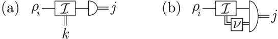
Figure 1: (a) Operational meaning of Eq. (5), where $\Lambda(t)={\cal I}_{k_{\ast}}$. (b) Discrimination problem in the case of the generalized erasure dynamics.

The operational meaning of Eq. (5) is depicted in Fig. 1(a). Let $p(j,k|i)$ be a joint probability to implement an operation ${\cal I}_{k}$ via a quantum instrument ${\cal I}$ and to observe the outcome $j$ while measuring the output quantum state, provided the input state is $\varrho_{i}$. Suppose ${\cal I}_{k_{\ast}}=\Lambda(t)$, then the maximum value of $\frac{1}{2}\sum_{i=1,2}p(j=i,k=k_{\ast}|i)$ exactly equals $p_{\rm succ.dist.}$ in Eq. (5).

3 System-ancilla entanglement dynamics

Suppose that in addition to the system of interest we also have access to an ancillary system, which is isolated from the decoherence sources. Provided the system dynamics is described by a trace preserving dynamical map $\Phi(t)$, the total system-ancilla aggregate undergoes an evolution given by the dynamical map $\Phi(t)\otimes{\rm Id}$, see Fig. 2(a).

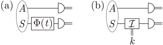
Figure 2: (a) Joint trace preserving dynamics of the system ($S$) and the ancilla ($A$). (b) Schematic of an experiment with trace decreasing dynamics, ${\cal I}_{k_{\ast}}=\Lambda(t)$.

Suppose that the system and the ancilla are initially entangled, then the system-ancilla entanglement generally changes in time. To quantify the system-ancilla entanglement, we use some entanglement monotone ${\cal E}$ that does not increase under trace preserving local operations and classical communication [27]. A seminal observation of Ref. [21] is that the entanglement monotone ${\cal E}(t)$ is a nonincreasing function of time $t$ provided the trace preserving map $\Phi(t)$ is CP-divisible. Any increase in ${\cal E}(t)$ is an indication of CP-indivisibility (non-Markovianity according to Ref. [19]). Although this approach to CP-indivisibility detection is absolutely legitimate in the case of trace preserving dynamical maps, it turns out to be wrong if one tracks the entanglement dynamics of postselected system-ancilla states [see setup in Fig. 2(b) with postselection $k=k_{\ast}$]. The following example justifies this claim.

Example 3.1.

Consider the polarization dependent losses that are time dependent too, i.e., the master equation of the form

$$\frac{d\varrho(t)}{dt}=-\frac{1}{2}\Big{\{}\gamma_{H}(t)\ket{H}\bra{H}+\gamma_{V}(t)\ket{V}\bra{V},\varrho(t)\Big{\}}.$$ (6)

A solution of this master equation is

$$\Lambda(t)[\varrho(0)]\equiv\varrho(t)=\left(\begin{array}[]{cc}e^{-\Gamma_{H}(t)}\varrho_{HH}(0)&e^{-\frac{1}{2}[\Gamma_{H}(t)+\Gamma_{V}(t)]}\varrho_{HV}(0)\\ e^{-\frac{1}{2}[\Gamma_{H}(t)+\Gamma_{V}(t)]}\varrho_{VH}(0)&e^{-\Gamma_{V}(t)}\varrho_{VV}(0)\\ \end{array}\right),$$

where $\Gamma_{H}(t)=\int_{0}^{t}\gamma_{H}(t^{\prime})dt^{\prime}$ and $\Gamma_{V}(t)=\int_{0}^{t}\gamma_{V}(t^{\prime})dt^{\prime}$. If $\gamma_{H}(t)$ and $\gamma_{V}(t)$ are both nonnegative, then the trace decreasing dynamical map $\Lambda(t)$ is CP-divisible.

Let us consider the specific rates

$$\gamma_{H}(t)=\gamma\left(1-\frac{\omega\cos\omega t}{\sqrt{\gamma^{2}+\omega^{2}}+\gamma\sin\omega t}\right),$$ (7)

$$\gamma_{V}(t)=\gamma\left(1+\frac{\omega\cos\omega t}{\sqrt{\gamma^{2}+\omega^{2}}-\gamma\sin\omega t}\right),$$ (8)

such that $\gamma_{H}(t)\geq 0$ and $\gamma_{V}(t)\geq 0$ if $\gamma>0$, $\omega>0$. Then

$$p_{H}(t):=e^{-\Gamma_{H}(t)}=e^{-\gamma t}\left(1+\frac{\gamma}{\sqrt{\gamma^{2}+\omega^{2}}}\sin\omega t\right),$$ (9)

$$p_{V}(t):=e^{-\Gamma_{V}(t)}=e^{-\gamma t}\left(1-\frac{\gamma}{\sqrt{\gamma^{2}+\omega^{2}}}\sin\omega t\right)$$ (10)

are both nonincreasing functions of time $t$. The physical meaning of $p_{H}(t)$ is the probability to successfully detect the horizontally polarized photon at time $t$ provided the photon was initially horizontally polarized. Eq. (10) has a similar meaning for vertically polarized photons. CP-divisibility of $\Lambda(t)$ means that the time evolution can be represented as a sequence of independent subevolutions, with each of them being a valid trace decreasing quantum operation. In this example, all the subevolutions are polarization dependent losses with different attenuation factors.

Let $\ket{\psi_{+}}\bra{\psi_{+}}$ be a maximally entangled initial state of the qubit system and a two-dimensional ancilla. This is exactly the case in the experimental scenario of Ref. [8], where the system-ancilla polarization state of two photons is produced via the spontaneous parametric down-conversion process. To be precise, $\ket{\psi_{+}}=\frac{1}{\sqrt{2}}(\ket{H}\otimes\ket{H}+\ket{V}\otimes\ket{V})$. The system-ancilla trace decreasing and CP-divisible dynamics $\Lambda(t)\otimes{\rm Id}[\ket{\psi_{+}}\bra{\psi_{+}}]$ results in the following conditional dynamics:

$$\frac{\Lambda(t)\otimes{\rm Id}[\ket{\psi_{+}}\bra{\psi_{+}}]}{{\rm tr}\big{[}\Lambda(t)\otimes{\rm Id}[\ket{\psi_{+}}\bra{\psi_{+}}]\big{]}}=\ket{\varphi(t)}\bra{\varphi(t)},$$ (11)

$$\ket{\varphi(t)}=\frac{1}{\sqrt{p_{H}(t)+p_{V}(t)}}\left(\sqrt{p_{H}(t)}\ket{H}\otimes\ket{H}+\sqrt{p_{V}(t)}\ket{V}\otimes\ket{V}\right).$$ (12)

Note that the conditional system-ancilla state remains pure for all times $t\geq 0$, so its entanglement is readily quantified by an entanglement monotone called concurrence [28]. We use that quantifier for our results to be comparable with Ref. [8], where the dynamics of concurrence is analyzed by an experimental reconstruction of the conditional system-ancilla states at different time moments. In our example, we have

$${\cal E}(t)=\frac{2\sqrt{p_{H}(t)p_{V}(t)}}{p_{H}(t)+p_{V}(t)}=\sqrt{\frac{\gamma^{2}\cos^{2}\omega t+\omega^{2}}{\gamma^{2}+\omega^{2}}},$$ (13)

which is clearly a nonmonotonic function of time if $\gamma>0$, $\omega>0$. Note that $\max_{t\geq 0}{\cal E}(t)={\cal E}(\frac{\pi n}{\omega})=1$ and $\min_{t\geq 0}{\cal E}(t)={\cal E}(\frac{\pi}{2\omega}+\frac{\pi n}{\omega})=\frac{\omega}{\sqrt{\gamma^{2}+\omega^{2}}}$, $n\in\mathbb{N}$, so there are infinitely many time periods of the entanglement increase (see the upper solid line in Fig. 3). The minimum value $\min_{t\geq 0}{\cal E}(t)$ can be arbitrarily close to 0 if $\omega\ll\gamma$. $\triangle$

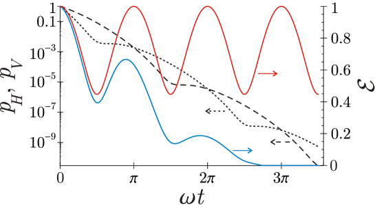
Figure 3: Monotonic dynamics of the probability $p_{H}$ (dashed line) and the probability $p_{V}$ (dotted line) in the trace decreasing CP-divisible evolution governed by the master equation (6) for polarization dependent losses; the rates $\gamma_{H}(t)$ and $\gamma_{V}(t)$ are given by Eq. (7) and Eq. (8), respectively, where $\gamma=2\omega$. Nonmonotonic dynamics of the concurrence ${\cal E}$ for the normalized system-ancilla state in Example 3.1 with $\gamma=2\omega$ (upper solid line), Eq. (13). Nonmonotonic dynamics of the concurrence ${\cal E}$ for the normalized system-ancilla state in Example 3.2 with $\gamma=2\omega$ and the depolarization rate $\lambda=0.05\omega$ (lower solid line).

Therefore, the entanglement increase in the experimentally reconstructed postselected system-ancilla state cannot be a valid indicator of CP-indivisibility (non-Markovianity) for trace decreasing dynamical maps. This fact was overlooked in Ref. [8].

The dynamical map $\Lambda(t)$ considered in Example 3.1 has Kraus rank 1, which preserves the purity of the postselected state. In the following example, we consider a more sophisticated dynamics, where the conditional system-ancilla state becomes mixed.

Example 3.2.

Suppose the polarization dependent losses in Example 3.1 are accompanied by a standard depolarization with the rate $\lambda>0$. Then the master equation takes the form

$$\frac{d\varrho(t)}{dt}=-\frac{1}{2}\Big{\{}\gamma_{H}(t)\ket{H}\bra{H}+\gamma_{V}(t)\ket{V}\bra{V},\varrho(t)\Big{\}}+\frac{\lambda}{4}\sum_{i=1}^{3}\big{(}\sigma_{i}\varrho(t)\sigma_{i}-\varrho(t)\big{)},$$ (14)

where $\gamma_{H}(t)$ and $\gamma_{V}(t)$ are given by Eqs. (7) and (8), respectively; $(\sigma_{1},\sigma_{2},\sigma_{3})$ is the conventional set of Pauli operators, i.e., $\sigma_{1}=\ket{H}\bra{V}+\ket{V}\bra{H}$, $\sigma_{2}=-i\ket{H}\bra{V}+i\ket{V}\bra{H}$, $\sigma_{3}=\ket{H}\bra{H}-\ket{V}\bra{V}$. Eq. (14) defines a trace decreasing CP-divisible dynamical map $\Lambda(t)$. The analytical expression for the postselected state $\Lambda(t)\otimes{\rm Id}[\ket{\psi_{+}}\bra{\psi_{+}}]/{\rm tr}\big{[}\Lambda(t)\otimes{\rm Id}[\ket{\psi_{+}}\bra{\psi_{+}}]\big{]}$ is rather involved though straightforward. We depict the postselected state concurrence ${\cal E}(t)$ for the particular choice of parameters $\gamma$, $\omega$, and $\lambda$ in Fig. 3 (see the lower solid line). The concurrence ${\cal E}(t)$ is a nonmonotonic function of time $t$ despite the fact that $\Lambda(t)$ is CP-divisible. $\triangle$

We can make another important observation in Fig. 3: If the depolarization rate is strictly positive in Example 3.2 (i.e., $\lambda>0$), then the concurrence ${\cal E}(t)$ vanishes at some time moment and remains zero after. In what follows we prove that this is a general phenomenon.

Proposition 3.3.

Let $\Lambda(t)$ be a trace decreasing CP-divisible dynamical map and $\varrho_{SA}(0)$ be an initial system-ancilla state. If the postselected system-ancilla state $\Lambda(t_{\ast})\otimes{\rm Id}[\varrho_{SA}(0)]/{\rm tr}\big{[}\Lambda(t_{\ast})\otimes{\rm Id}[\varrho_{SA}(0)]\big{]}$ becomes separable at time moment $t_{\ast}$, then all future postselected states ($t\geq t_{\ast}$) remain separable.

Proof 3.4.

Since the postselected system-ancilla state is separable at time $t_{\ast}$, we have $\Lambda(t_{\ast})\otimes{\rm Id}[\varrho_{SA}(0)]/{\rm tr}\big{[}\Lambda(t_{\ast})\otimes{\rm Id}[\varrho_{SA}(0)]\big{]}=\sum_{i}p_{i}\varrho_{S}^{(i)}\otimes\varrho_{A}^{(i)}$, where $\{p_{i}\}_{i}$ is a probability distribution, $\{\varrho_{S}^{(i)}\}_{i}$ and $\{\varrho_{A}^{(i)}\}_{i}$ are the sets of density operators for the system and the ancilla, respectively. Let $t\geq t_{\ast}$. Since $\Lambda(t)$ is CP-divisible, then there exists a map $\Theta(t,t_{\ast})$ such that $\Lambda(t)=\Theta(t,t_{\ast})\Lambda(t_{\ast})$. Hence,

$$\frac{\Lambda(t)\otimes{\rm Id}[\varrho_{SA}(0)]}{{\rm tr}\big{[}\Lambda(t)\otimes{\rm Id}[\varrho_{SA}(0)]\big{]}}=\sum_{i}q_{i}\frac{\Theta(t,t_{\ast})[\varrho_{S}^{(i)}]}{{\rm tr}\left[\Theta(t,t_{\ast})[\varrho_{S}^{(i)}]\right]}\otimes\varrho_{A}^{(i)},$$

$$q_{i}=\frac{p_{i}{\rm tr}\left[\Theta(t,t_{\ast})[\varrho_{S}^{(i)}]\right]}{\sum_{j}p_{j}{\rm tr}\left[\Theta(t,t_{\ast})[\varrho_{S}^{(j)}]\right]},$$

i.e., the postselected state at time moment $t\geq t_{\ast}$ is separable too. $\square$

Corollary 3.5.

Suppose the system experiences a trace decreasing dynamics $\Lambda(t)$. The system-ancilla entanglement death followed by the entanglement revival is an indication of CP-indivisibility for $\Lambda(t)$.

Using the results of Ref. [29], the above claims can be reformulated and generalized in terms of the Schmidt rank as follows: A CP-divisible trace decreasing system dynamics $\Lambda(t)$ does not increase the Schmidt rank of the system-environment normalized states $\Lambda(t)\otimes{\rm Id}[\varrho_{SA}(0)]/{\rm tr}\big{[}\Lambda(t)\otimes{\rm Id}[\varrho_{SA}(0)]\big{]}$.

Clearly, the examples and the statements above hold true not only for continuous time evolutions but also in the case of the discrete time evolutions, e.g., collision models that are reviewed in Ref. [30].

4 Generalized erasure dynamics

In Ref. [17], a generalized erasure channel has been introduced as a physically motivated extension of a trace decreasing operation. In fact, the successful implementation of a quantum operation $\Lambda$ for an input state $\varrho$ happens with the probability ${\rm tr}\big{[}\Lambda[\varrho]\big{]}$, so the failure probability equals

$$p_{\rm fail}=1-{\rm tr}\big{[}\Lambda[\varrho]\big{]}={\rm tr}\big{[}\varrho-\Lambda[\varrho]\big{]}={\rm tr}\left[\left(I-\Lambda^{{\dagger}}[I]\right)\varrho\right],$$ (15)

where $\Lambda^{{\dagger}}$ is a dual map with respect to $\Lambda$ such that ${\rm tr}\big{[}\Lambda[X]Y\big{]}={\rm tr}\big{[}X\Lambda^{{\dagger}}[Y]\big{]}$ for all trace-class operators $X$ and bounded operators $Y$. The probability $p_{\rm fail}$ is readily accessible in a physical experiment. For instance, in the experimental setup of Ref. [8], this probability can be evaluated as $(N_{A}-N_{S})/N_{S}$, where $N_{A}$ is a number of the detector clicks for the ancilla and $N_{S}$ is a number of the detector clicks for the system, see Fig. 2(b). Although this extra information is free, it is usually disregarded in the postselection-oriented experiments. We argue that the unsuccessful implementation of operation $\Lambda$ can be viewed as an erasure event. In Fig. 2(b), this event is associated with the click of the ancilla detector and no click of the system detector. We extend the Hilbert space and include the erasure flag state $\ket{e}$ into it so that the map

$$\Gamma_{\Lambda}[\varrho]=\Lambda[\varrho]\oplus{\rm tr}\left[\left(I-\Lambda^{{\dagger}}[I]\right)\varrho\right]\ \ket{e}\bra{e}\equiv\left(\begin{array}[]{cc}\Lambda[\varrho]&{\bf 0}\\ {\bf 0}^{\top}&{\rm tr}\left[\left(I-\Lambda^{{\dagger}}[I]\right)\varrho\right]\\ \end{array}\right)$$ (16)

is trace preserving and completely positive [17]. Therefore, any trace decreasing dynamics $\Lambda(t)$ can be alternatively described by virtue of the corresponding trace preserving dynamical map $\Gamma_{\Lambda}(t)\equiv\Gamma_{\Lambda(t)}$. We refer to $\Gamma_{\Lambda}(t)$ as the generalized erasure dynamics.

CP-indivisibility identification problems discussed in Secs. 2 and 3 were caused by the postselection. Instead, if we use the generalized erasure dynamics, then those problems are automatically resolved.

Proposition 4.1.

Suppose $\Lambda(t)$ is a CP-divisible trace decreasing dynamical map, then $\Gamma_{\Lambda}(t)$ is a CP-divisible trace preserving dynamical map.

Proof 4.2.

Let $t_{2}\geq t_{1}\geq 0$, then $\Lambda(t_{2})=\Theta(t_{2},t_{1})\Lambda(t_{1})$, where $\Theta(t_{2},t_{1})$ is a quantum operation. Consider the map

$$\Xi(t_{2},t_{1})\left[\left(\begin{array}[]{cc}\varrho&\vdots\\ \cdots&c\\ \end{array}\right)\right]=\left(\begin{array}[]{cc}\Theta(t_{2},t_{1})[\varrho]&{\bf 0}\\ {\bf 0}^{\top}&c+{\rm tr}\left[\rho(I-\Theta(t_{2},t_{1})^{{\dagger}}[I])\right]\\ \end{array}\right),$$ (17)

which is automatically trace preserving and, in addition, completely positive because a quantum operation $\Theta(t_{2},t_{1})$ is trace nonincreasing, i.e., $\Theta(t_{2},t_{1})^{{\dagger}}[I]\leq I$. We have $\Gamma_{\Lambda}(t_{2})=\Xi(t_{2},t_{1})\Gamma_{\Lambda}(t_{1})$, i.e., $\Gamma_{\Lambda}(t)$ is CP-divisible. $\square$

Due to Proposition 4.1, the distinguishability of equiprobable states $\Gamma_{\Lambda}(t)[\varrho_{1}]$ and $\Gamma_{\Lambda}(t)[\varrho_{2}]$ monotonically decreases if $\Lambda(t)$ is CP-divisible. Remarkably, the probability to successfully distinguish these states, $\frac{1}{2}+\frac{1}{4}\|\Gamma_{\Lambda}(t)[\varrho_{1}]-\Gamma_{\Lambda}(t)[\varrho_{2}]\|_{1}$, exceeds the probability (5) by $\frac{1}{2}\left(1-\min_{i=1,2}{\rm tr}\big{[}\Lambda(t)[\varrho_{i}]\big{]}\right)$ because the modified scenario takes into account the erasure events too [see Fig. 1(b), where $\nu$ is a coarse-graining postprocessing with two outcome events: $k=k_{\ast}$ and $k\neq k_{\ast}$].

Similarly, Proposition 4.1 implies that the system-ancilla entanglement monotonically decreases during the trace preserving dynamics $\Gamma_{\Lambda}(t)\otimes{\rm Id}$ if $\Lambda(t)$ is CP-divisible.

5 Conclusions

In the present work, we have paid attention to some simple yet important questions of how to analyze the divisibility problem in experiments that involve postselection. By a number of examples we have demonstrated the complete inconsistency of some approaches that operate with the postselected states as though they were obtained as a result of a trace preserving dynamics. In particular, none of the Eqs. (1) and (3) is adequate in the analysis of the information backflow because either of these quantities can increase during a CP-divisible dynamics. The original idea behind the information backflow is properly described by Eq. (5) that has a clear physical meaning. Similarly, we show that the increase in the system-ancilla entanglement is not a valid indicator of CP-indivisibility if the postselection takes place. Unfortunately, these facts are sometimes overlooked in research papers, e.g., a nonmonotonic concurrence behavior for the system-ancilla postselected state was mistreated as an indicator of non-Markovianity in the paper [8] (this paper has an extra drawback related with non-unitarity of the inter-environment collision that we do not discuss in this work). We advocate that a correct indicator of non-Markovianity should be related with an increase of the system-ancilla Schmidt rank, e.g., the revival of the entanglement after the entanglement death (Corollary 3.5). A general analysis of the two-qubit entanglement dynamics under local trace decreasing maps can be accomplished by following the lines of Ref. [31] and using the quantum Sinkhorn theorem. Finally, we have described the framework of generalized erasure dynamics that takes into account how often a desired trace decreasing operation is actually implemented and how often the implementation fails. This extra information is readily available in experiments though it is rarely used. On the other hand, including this information into the description allows us to return to the fold of trace preserving maps. Those trace preserving maps inherit some properties of the original operations, e.g., CP-divisibility (Proposition 4.1). Moreover, the induced trace preserving maps have an interesting property of superadditivity of coherent information [17].

References

- [1] U’Ren, A. B., Silberhorn, C., Banaszek, K., Walmsley, I. A.: Efficient conditional preparation of high-fidelity single photon states for fiber-optic quantum networks. Phys. Rev. Lett. 93, 093601 (2004).
- [2] Kiesel, N., Schmid, C., Weber, U., Ursin, R., Weinfurter, H.: Linear optics controlled-phase gate made simple. Phys. Rev. Lett. 95, 210505 (2005).
- [3] Kovlakov, E. V., Straupe, S. S., Kulik, S. P.: Quantum state engineering with twisted photons via adaptive shaping of the pump beam. Phys. Rev. A 98, 060301(R) (2018).
- [4] Wenger, J., Tualle-Brouri, R., Grangier, P.: Non-Gaussian statistics from individual pulses of squeezed light. Phys. Rev. Lett. 92, 153601 (2004).
- [5] Bogdanov, Yu. I., Katamadze, K. G., Avosopiants, G. V., Belinsky, L. V., Bogdanova, N. A., Kalinkin, A. A., Kulik, S. P.: Multiphoton subtracted thermal states: description, preparation, and reconstruction. Phys. Rev. A 96, 063803 (2017).
- [6] Zavatta, A., Viciani, S., Bellini, M.: Quantum-to-classical transition with single-photon-added coherent states of light. Science 306, 660-662 (2004).
- [7] Pryde, G. J., O’Brien, J. L., White, A. G., Ralph, T. C., Wiseman, H. M.: Measurement of quantum weak values of photon polarization. Phys. Rev. Lett. 94, 220405 (2005).
- [8] Cuevas, Á., Geraldi, A., Liorni, C., Bonavena, L. D., De Pasquale, A., Sciarrino, F., Giovannetti, V., Mataloni, P.: All-optical implementation of collision-based evolutions of open quantum systems. Sci. Rep. 9, 3205 (2019).
- [9] Kraus, K.: States, Effects, and Operations. Springer-Verlag, Berlin (1983).
- [10] Davies, E. B., Lewis, J. T.: An operational approach to quantum probability. Comm. Math. Phys. 17, 239-260 (1970).
- [11] Holevo, A. S.: Quantum Systems, Channels, Information. A Mathematical Introduction. De Gruyter, Berlin, Boston (2012).
- [12] Heinosaari, T., Ziman, M.: The Mathematical Language of Quantum Theory. Cambridge Univ. Press, Cambridge (2012).
- [13] Filippov, S. N.: On quantum operations of photon subtraction and photon addition. Lobachevskii J. Math. 40, 1470-1478 (2019).
- [14] Bongioanni, I., Sansoni, L., Sciarrino, F., Vallone, G., Mataloni, P.: Experimental quantum process tomography of non-trace-preserving maps. Phys. Rev. A 82, 042307 (2010).
- [15] Luchnikov, I. A., Filippov, S. N.: Quantum evolution in the stroboscopic limit of repeated measurements. Phys. Rev. A 95, 022113 (2017).
- [16] Grimaudo, R., Messina, A., Sergi, A., Vitanov, N. V., Filippov, S. N.: Two-qubit entanglement generation through non-Hermitian Hamiltonians induced by repeated measurements on an ancilla. Entropy 22, 1184 (2020).
- [17] Filippov, S. N.: Capacity of trace decreasing quantum operations and superadditivity of coherent information for a generalized erasure channel. J. Phys. A: Math. Theor. 54, 255301 (2021).
- [18] Gisin, N., Huttner, B.: Combined effects of polarization mode dispersion and polarization dependent losses in optical fibers. Optics Communications 142, 119 (1997).
- [19] Rivas, Á., Huelga, S. F., Plenio, M. B.: Quantum non-Markovianity: characterization, quantification and detection. Rep. Prog. Phys. 77, 094001 (2014).
- [20] Chruściński, D., Rivas, Á., Størmer, E.: Divisibility and information flow notions of quantum Markovianity for noninvertible dynamical maps. Phys. Rev. Lett. 121, 080407 (2018).
- [21] Rivas, Á., Huelga, S. F., Plenio, M. B.: Entanglement and non-Markovianity of quantum evolutions. Phys. Rev. Lett. 105, 050403 (2010).
- [22] Chruściński, D., Macchiavello, C., Maniscalco, S.: Detecting non-Markovianity of quantum evolution via spectra of dynamical maps. Phys. Rev. Lett. 118, 080404 (2017).
- [23] Filippov, S. N., Chruściński, D.: Time deformations of master equations. Phys. Rev. A 98, 022123 (2018).
- [24] Breuer, H.-P., Laine, E.-M., Piilo, J.: Measure for the degree of non-Markovian behavior of quantum processes in open systems. Phys. Rev. Lett. 103, 210401 (2009).
- [25] Milz, S., Kim, M. S., Pollock, F. A., Modi, K.: Completely positive divisibility does not mean Markovianity. Phys. Rev. Lett. 123, 040401 (2019).
- [26] Ruskai, M. B.: Beyond strong subadditivity? Improved bounds on the contraction of generalized relative entropy. Rev. Math. Phys. 6, 1147-1161 (1994).
- [27] Plenio, M. B., Virmani, S.: An introduction to entanglement measures. Quant. Inform. Comput. 7, 1 (2007).
- [28] Hill, S., Wootters, W. K.: Entanglement of a pair of quantum bits. Phys. Rev. Lett. 78, 5022 (1997).
- [29] Sperling, J., Vogel, W.: The Schmidt number as a universal entanglement measure. Phys. Scr. 83, 045002 (2011).
- [30] Campbell, S., Vacchini, B.: Collision models in open system dynamics: A versatile tool for deeper insights? EPL 133, 60001 (2021).
- [31] Filippov, S. N., Frizen, V. V., Kolobova, D. V.: Ultimate entanglement robustness of two-qubit states against general local noises. Phys. Rev. A 97, 012322 (2018).